the Creative Commons Attribution 4.0 License.
the Creative Commons Attribution 4.0 License.
 | 02 Oct 2019
Improving the quality of empirical Green's functions, obtained by cross-correlation of high-frequency ambient seismic noise
Elena Kozlovskaya
Jouni Nevalainen
Janne Narkilahti
Studying the uppermost structure of the subsurface is a necessary part of solving many practical problems (exploration of minerals, groundwater studies, geoengineering, etc.). The practical application of active seismic methods for these purposes is not always possible for different reasons, such as logistical difficulties, high cost of work, and a high level of seismic and acoustic noise. That is why developing and improving passive seismic methods is one of the important problems in applied geophysics. In our study, we describe a way of improving the quality of empirical Green's functions (EGFs), evaluated from high-frequency ambient seismic noise, by using the advanced technique of cross-correlation function stacking in the time domain (in this paper we use term “high-frequency” for frequencies higher than 1 Hz). The technique is based on the global optimization algorithm, in which the optimized objective function is a signal-to-noise ratio of an EGF, retrieved at each iteration. In comparison to existing techniques, based, for example, on weight stacking of cross-correlation functions, our technique makes it possible to significantly increase the signal-to-noise ratio and, therefore, the quality of the EGFs. The technique has been tested with the field data acquired in an area with a high level of industrial noise (Pyhäsalmi Mine, Finland) and in an area with a low level of anthropogenic noise (Kuusamo Greenstone Belt, Finland). The results show that the proposed technique can be used for the extraction of EGFs from high-frequency seismic noise in practical problems of mapping of the shallow subsurface, both in areas with high and low levels of high-frequency seismic noise.
- Article
(6644 KB) - Full-text XML
- BibTeX
- EndNote


Seismic methods as tools for studying the shallow subsurface structures in exploration geophysics have been developed for many years. Traditionally, seismic surveys (reflection and refraction) have been carried out using active sources. The reflection and refraction controlled-source seismic sounding methods are widely applied in exploration for oil and gas but less commonly in mineral exploration in crystalline bedrock areas. The reasons for this have been the traditionally high cost of seismic surveys and logistical difficulties (Malehmir et al., 2012). Seismic methods as a mineral exploration tool are very good for delineation of the boundaries of certain types of mineral deposits as well as for estimating their ore potential (Kukkonen et al., 2009; Malehmir et al., 2012). There are, however, challenges in exploration of new deep targets in the vicinity of active mines, that is, in brownfield exploration. In our paper, brownfield means exploration near active mines or at the previously studied area with the purpose of getting new mineral reserves, while greenfield means exploration of new mineral deposits. Due to the large amount of heavy machinery, the active mines themselves produce strong seismic and acoustic noise. This continuous noise overlaps in frequencies with the signals of the controlled seismic sources, creating a problem for the high-resolution active-source seismic experiments in a brownfield exploration (Place et al., 2015).
In our paper, we describe results of investigating the possibility of using passive ambient seismic noise interferometry with the noise with frequencies higher than 1 Hz (hereafter, we use the term “high-frequency” for this seismic noise) for extracting information about the shallow subsurface in greenfield and brownfield exploration projects. In our study, the shallow subsurface means depths from ground surface down to several hundreds metres. For this, we develop a new method of improving the quality of empirical Green's function (EGFs) evaluated from high-frequency industrial, anthropogenic or natural seismic noise. We partly use algorithms described in Shapiro et al. (2005), Campillo (2006), Bensen et al. (2007), Groos et al. (2012), Poli et al. (2012a, b, 2013), and Afonin et al. (2017) for ambient noise preprocessing and implement a new algorithm of stacking cross-correlation functions in the time domain.
At present, there are several advanced algorithms, working in the time domain, in the frequency domain or in the time–frequency domain. One group of algorithms tries to improve the quality of the resulting EGFs using the evaluation of cross-correlation functions according to certain criteria prior to stacking them. For example, in the methods described in Baig et al. (2009), a denoising procedure, based on S transform, is applied to cross-correlation functions before their stacking. In the “time–frequency domain phase-weighted stacking” method, which may use either S transform (Schimmel et al., 2011) or wavelet transform (Ventosa et al., 2017), phases of signals are analysed prior stacking them. The errors that inverse S transforms may introduce to subsequent phase-velocity measurements were analysed in Li et al. (2018). Another approach, based on stacking only cross-correlation functions of highly coherent signals, was used in global-scale coda wave interferometry studies (Boué et al., 2014). These algorithms do not use signal-to-noise ratios (SNRs) of cross-correlation functions for improving the final EGF, and it is assumed that signal coherence by itself is a guarantee that all non-suitable cross-correlation functions are either excluded from the final stack or minimized by using weights, and hence the SNR is automatically improved. This may be true for teleseismic coda wave interferometry (Phạm et al., 2018), in which source location is a priori known and it is easy to control that only signals within the so-called “stationary phase” area are cross-correlated (Wapenaar et al., 2010). However, in the ambient noise studies with noise sources that are stochastically and non-evenly distributed in time and space their azimuthal distribution is not known a priori. In this case, one would need to take into account this distribution, in order to satisfy the stationary phase condition. The other group of methods, such as “root mean square stacking” or weight stacking (Shirzad and Shomali, 2015; Nakata et al., 2015; Cheng et al., 2015; Li et al., 2018) are aiming mainly at increasing a signal-to-noise ratio of the resulting EGF, but they do not take into account the coherence of the cross-correlation functions in the stack. That is why incoherent cross-correlation functions are not totally excluded from the stack in these algorithms, and this can decrease the quality of evaluated EGFs.
To overcome the limitations of existing techniques, we develop a new algorithm that makes it possible not only to exclude incoherent cross-correlation functions from the EGF stacking process but also to keep control of the azimuthal distribution of noise sources and the condition of the stationary phase. In our paper the term “coherent” is used to define cross-correlation functions with the same time lags of signal maxima and the same dominant frequency. We do not use this method in the frequency domain because for stationary phase condition to be satisfied, it is important to stack cross-correlation functions with the same time lags and dominant frequencies, in other words, functions that are coherent with each other. As a main criterion for selecting cross-correlation functions to stack, we use an increase in the SNR of extracted EGFs after stacking. Moreover, we use the global optimization algorithm for obtaining the best solution for the SNR. In this case, an SNR, calculated on each iteration, is an objective function that is optimized.
In our paper, we present details of this algorithm and illustrate its performance using passive seismic ambient noise data acquired in two areas of Fennoscandia: Pyhäsalmi mine (as an example of area with a high level of industrial noise) and the Kuusamo Greenstone Belt area (a quiet area prospective for new mining projects (Weihed et al., 2005; Lehtonen and O'Brien, 2009).
For solving the problems described in the “Introduction” section, we suggest our method of time-domain stacking of cross-correlation functions calculated for different time windows. We call this method SNR stacking. The general purpose of this method is to select for stacking only those cross-correlation functions that are not only coherent with each other but also correspond to the stationary phase area.
Let us assume that ambient noise in a particular frequency band is recorded simultaneously at two different points with Cartesian coordinates r1 and r2. For each frequency, the stationary phase area for the receiver located at the point ri, i=1, 2 corresponds to the Fresnel zone of the wave propagating from the source to the receiver with a particular apparent velocity. In this case, the maximum of the cross-correlation function at a particular time lag would correspond to the minimum of apparent velocity, and hence, the cross-correlation function would be close to the “true” EGF. We assume that noise sources are partly located in a stationary phase area while other noise sources are distributed outside it. For the selection of cross-correlation functions corresponding to the stationary phase area, it is possible to use criteria of minimum apparent velocity and of the signal-to-noise ratio increasing after stacking. We consider the SNR of the EGF after stacking as a particular, generally non-linear function of apparent velocity and a back-azimuth of noise sources and an initial time window used to start the selection of cross-correlation functions to the stack. In this case, the global optimization of this objective function would allow us to retrieve EGFs of high quality.
We assume again that the ambient seismic noise is recorded simultaneously at two different points with Cartesian coordinates r1 and r2, r=[xyz], and continuous recordings are split into n time windows with the same durations. Let ai(r1r2t) be the cross-correlation function of these seismic records for the time window i, i=1…n, where t is a time lag of the seismic records. Let tm be the maximum time lag in a cross-correlation function (length of cross-correlation); tds is a maximum time of wave propagation between the two points; |tm|≫|tds| and . Let be the time lag on the cross-correlation function corresponding to the expected seismic phase (body or surface wave) and , where T is the period of expected signal. Negative values of the time lags correspond to the anti-casual part of the evaluated EGF. In this case, the selection of tds and te is based upon a priori information about seismic velocities in the studied area. The value of te is at least two periods of the expected signal dominant frequency. In the case of the evaluation of surface wave parts of EGFs, this frequency usually corresponds to the frequency of noise with the largest amplitude that can be estimated by time–frequency analysis of the seismic noise records.
Let be the maximum value of cross-correlation function in the time interval te. Then, the signal-to-noise ratio of the cross-correlation function calculated for the ith time window (SNR(ai(r1r2t))) is
Let ai(r1r2t) and aj(r1r2t) be cross-correlation functions calculated for two different time windows i∈(1…n), and j∈(1…n) and are an EGF retrieved from these two cross-correlation functions. If and are coherent with each other and i≠j, then the expressions and have to be true, according to the principle of interference. The condition i≠j is necessary in order to avoid stacking of functions with themselves. Therefore, increasing the SNR of the retrieved EGF after stacking with a particular cross-correlation function can be used as a criterion for the selection of this function to the stack, excluding incoherent functions from the stack and building up the EGF with a high signal-to-noise ratio.
Based on the criteria described above, an expression for the calculation of the EGF for the kth iteration can be written as
where k=1…n is the number of initial function; n is the number of time windows; ; is the EGF corresponding to kth initial function and evaluated in previous iterations:
The operator of selection can be written as
As a result of this algorithm we obtain n candidates for the EGF that can be considered as solutions to the optimization problem in a particular parameter space. Let us consider the signal-to-noise ratio as a particular function f(k), where k is the index of initial functions: . Then the condition for the final EGF selection can be written as m=argmax(f(k)), where m denotes the index of the EGF selected to the stack. Following this condition, the EGF with the maximum signal-to-noise ratio will be selected as the final one. As the function f(k) may have several local maxima in the parameter space k, , the condition for the final EGF selection ensures that the global maximum of this function is obtained in the parameter space considered.
In the proposed algorithm, maximizing the signal-to-noise ratio of the retrieved EGF is ensured by stacking only cross-correlation functions coherent with each other and the selection of the EGF with the maximum signal-to-noise ratio from all calculated candidate EGFs. In other words, the proposed algorithm is analogous to the direct search methods of global optimization. It is necessary to remember, however, that the EGF with the maximum signal-to-noise ratio does not correspond to a true EGF if the dominant noise sources are located outside the stationary phase area. Therefore, it is important to use the system of observations that allows estimating the azimuthal distribution of noise sources. Moreover, the method is based on the assumption that sources of the ambient seismic noise produce a signal with relatively broad bandwidth and cannot produce an ideal harmonic signal of single frequency.
The method also makes it possible to keep control over an a priori unknown azimuthal distribution of noise sources. For this, a 2-D array of seismic recording stations is necessary. In this case, the time lags, corresponding to the expected signal te in Eq. (1) have to be a function of apparent seismic velocity and back-azimuth: te=f(vφ). Then the signal-to-noise ratio for each pair of stations of the array is the function of the initial function index, velocity, and back-azimuth: . Limits of apparent velocities have to be calculated according to a priori information about seismic velocities in the studied area. A global maximum of the function corresponds to the strongest or the most coherent wave field. Therefore, the method allows estimating azimuth to the strongest source of noise wave field.
We suggest that this method can be used for the extraction of EGFs from high-frequency industrial, anthropogenic, or natural seismic noise. Moreover, this method does not require that only a diffuse field is used for calculating EGFs. Therefore, the application of this method to the data of optimally selected seismic recording array might significantly decrease the time necessary for the registration of ambient seismic noise, which is very important for practical applications of passive seismic interferometry. For studying the possibilities of using this method for the extraction of EGFs from high-frequency seismic noise, we use the data from two passive seismic experiments carried out in areas with different seismic noise characteristics. The first area is characterized by a high level of industrial noise (Pyhäsalmi underground mine site) that is usually observed in brownfield exploration areas, while the second area is seismically very quiet and is characterized by a limited amount of local anthropogenic (roads) and natural (rivers) high-frequency seismic noise sources. Such noise characteristics are typical of greenfield exploration areas.
3.1 Pyhäsalmi mine area
As an example of using a high-level industrial seismic noise for the estimation of EGFs, we used the seismic noise at the site of Pyhäsalmi mine, Finland. For this purpose we installed 24 three-component DSU-SA MEMS (microelectromechanical system) seismic sensors with the autonomous RAUD eX data acquisition units manufactured by Sercel Ltd (France). The instruments were installed along a 10 km long line crossing the mine area with interstation distances of about 100 m (for PLB03-PLB13 and PLB14-PLB22) and 2 km (PLB01, PLB02, PLB23, PLB24) (Fig. 1). The seismic stations recorded continuous seismic data from 1 to 5 November 2013 with a sampling frequency of 500 samples per second (sps).
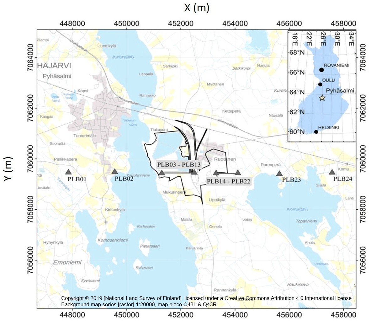
Figure 1Map of the experiment near the Pyhäsalmi mine in Universal Transverse Mercator coordinate system with the two parts of the profile (PLB01-PLB13 – west part of profile; PLB14-PLB24 – east part of profile). Black lines are the borders of the mine and open-pit territories. At locations PLB01, PLB02, PLB03, PLB13, PLB14, PLB22, PLB23, and PLB24 both MEMS and Trillium Compact sensors were installed.
The profile configuration was selected on the basis of the test measurements of ambient noise in the Pyhäsalmi area made by the authors. These studies showed that the mine is the main source of seismic high-frequency noise at distances about several kilometres from the mine.
The profile crossing the mine area consists of two parts, and each of these consists of 12 sensors: the western part has direction from the mine to the west (PLB01-PLB13), and the eastern part has direction from the mine to the east (PLB14-PLB24). Each part of the profile includes one sensor closest to the mine (PLB13 and PLB14). The horizontal components were oriented to the true north and east (N–S and E–W components, respectively). Thus, rotation of the horizontal components before seismic noise analysis was not necessary.
3.2 Kuusamo Greenstone Belt area
As an example of an area with a low level of anthropogenic seismic noise, we selected an area located in the Kuusamo Greenstone Belt (KuGB), Finland, because of numerous previous geological and geophysical studies there (Silvennoinen, 1991; Bruneton et al., 2004; Yliniemi et al., 2004; Silvennoinen and Kozlovskaya, 2007; Poli et al., 2012b; Pedersen et al., 2013; Silvennoinen et al., 2014; Tiira et al., 2014; Vinnik et al., 2014, etc.). Moreover, Weihed et al. (2005) and Lehtonen and O'Brien (2009) have shown that this area is prospective for gold- and diamond deposits.
For testing our method of cross-correlation function stacking, we use the data collected during a passive seismic experiment in the KuGB area in August and September 2014. One of the aims of this experiment was to investigate the possibility of high-frequency EGF extraction from anthropogenic or natural seismic noise in regions with a low ambient noise level.
The temporary seismic array (Fig. 2) consisted of five three-component velocimeters Trillium Compact produced by Nanometrics (Canada) and 24 three-component accelerometers DSU-SA MEMS with autonomous RAUD eX data acquisition units manufactured by Sercel Ltd.
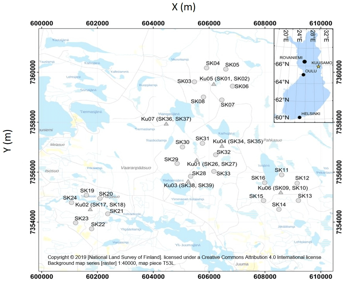
Figure 2Configuration of the temporary seismic array on Kuusamo area in Universal Transverse Mercator coordinate system: white triangles – positions of broadband sensors (Trillium compacts); white dots – positions of accelerometers (MEMS).
As one can see in Fig. 2, the seismic array represents a triangle. The sides of this triangle are about 4–6 km long. The broadband (BB) sensors were installed in the vertices of this triangle and collocated with MEMS accelerometers. In addition, each of these large triangle vertices was surrounded by a circular array with a small aperture (about 1400–1500 m), consisting of six accelerometers. The whole array recorded continuous seismic data from 28 August to 10 September 2014 with a sampling rate of 500 sps. Such an array configuration makes it possible to estimate the azimuthal distribution of the high-frequency noise sources and also to extract high-frequency EGFs from records of small aperture arrays.
4.1 Time–frequency analysis
One of the most important steps of the data preparation before the extraction of EGFs is the time–frequency analysis. It is necessary for the selection of a frequency band with high amplitudes of ambient noise. For this, we analysed characteristics of seismic noise recorded at different distances from the potential noise sources. In the Pyhäsalmi experiment, the most probable noise sources are located inside the underground mine and in the open pit. For the time–frequency analysis of the seismic noise, we used records of sensors installed at different distances from the mine and from the open pit (PLB24 and PLB14; Fig. 1). Figure 3a, b show the results of this analysis.
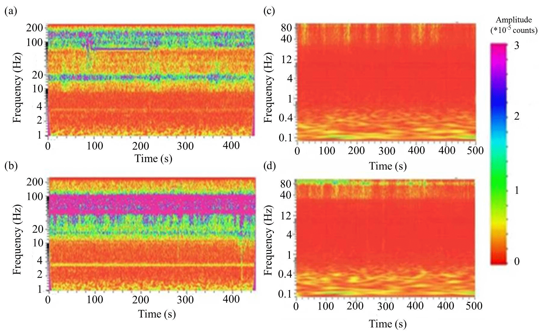
Figure 3Result of time–frequency analysis of seismic noise recorded by the sensor (a) the most distant from the mine in the Pyhäsalmi experiment, (b) closest to the mine in the Pyhäsalmi experiment, (c) most distant from a noise source (river) (KU05) in the large-aperture array in the Kuusamo experiment, and (d) KU02, which is closest to the river in the large-aperture array in the Kuusamo experiment.
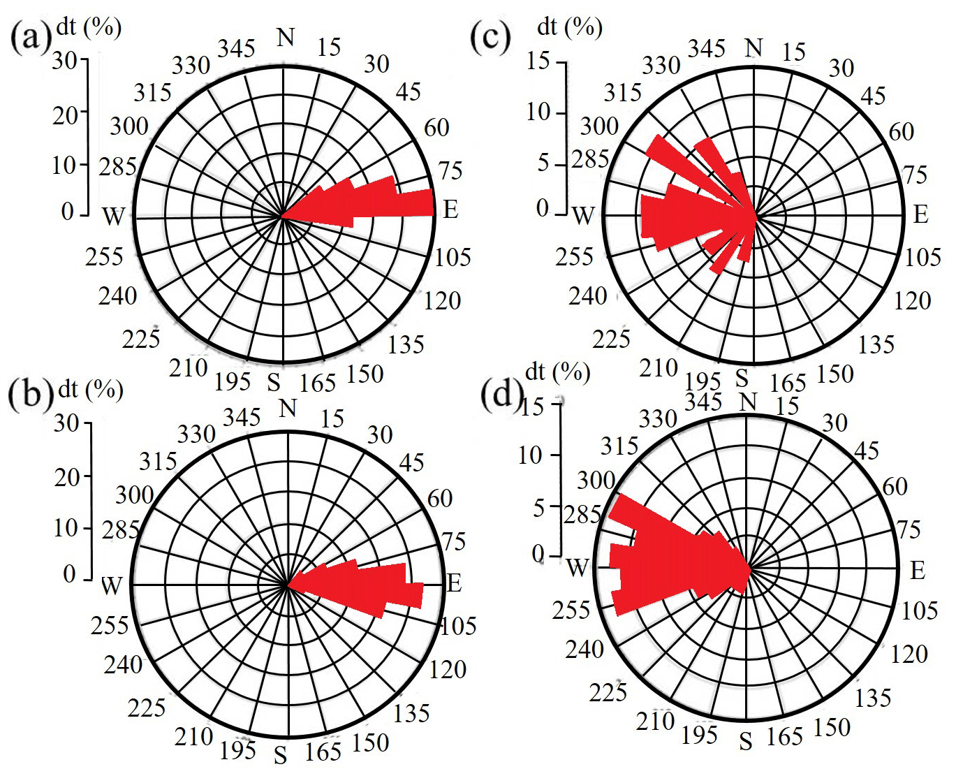
Figure 4Result of the azimuthal distribution calculation for different frequency bands for the Pyhäsalmi experiment: (a) west part of profile, band of 2–5 Hz; (b) west part of profile, band of 5–10 Hz; (c) east part of profile, band of 2–5 Hz; (d) east part of profile, band of 5–10 Hz.
From Fig. 3a, b, one can see two main frequency bands with high amplitudes of the seismic noise recorded closest to the mine: about 3–4 and about 10–100 Hz, respectively. Moreover, the amplitudes of the noise in these frequency bands decrease with distance from the mine. Therefore, we can assume that the sources of the noise for these frequency bands are located inside the underground mine and in the open pit. Based on this analysis, we selected the frequency band of 1–100 Hz for pre-filtering of the noise prior to the calculation of cross-correlation functions.
In the KuGB experiment, a temporary seismic network was installed in a quiet area without any significant industrial activity; therefore, we can assume that the high-frequency seismic noise might be produced by multiple natural (for example, rivers) and/or anthropogenic (for example, roads) sources. In this case, analysis of time–frequency characteristics of the seismic noise is a necessary step. For this, we calculated time–frequency diagrams in the frequency band of 0.1–100 Hz, and examples of these diagrams for two stations are presented in Fig. 3c, d.
Figure 3c, d show that noise records of both stations have amplitude maxima in the frequency band of 0.1–1 Hz. Seismic noise recorded by the KU05 station is also characterized by periodically high amplitudes in the frequency band of 40–100 Hz (Fig. 3c). This noise may be caused by anthropogenic (transport) or natural (for example, wind) sources. Station KU02 is located close to the river that can be a source of continuous seismic noise with high amplitudes in the frequency band of 40–80 Hz (Fig. 3d). Therefore, for the estimation of a high-frequency EGF, we pre-filtered the data with the band-pass filter of 1–100 Hz.
4.2 Analysis of the azimuthal distribution of the noise sources
Classical methods of passive seismic interferometry are based on diffuse field approximation (Wapenaar et al., 2008, 2010). One of the most important conditions for using this approximation is an isotropic and homogeneous azimuthal distribution of noise sources (Mulargia, 2012). That is why the second important procedure of data preparation before the estimation of EGFs is analysis of the azimuthal distribution of the noise sources during the experiment's period. In our study, we considered two cases. In the case of the Pyhäsalmi area, the main sources of high-frequency seismic noise are most probably located inside the mine and in the open pit. Thus, the assumption about an isotropic and homogeneous azimuthal distribution is not valid. As shown in Wapenaar et al. (2010), in such cases one cannot assume diffuse field approximations. That is why the measurements of the noise were made along a profile (linear array) consisting of two parts crossing the mine site and oriented E–W. However, signals from other noise sources outside the stationary field area can also be present in the wave field acquired during the data acquisition period. That is why we carried out additional analysis of the azimuthal distribution of noise sources. For the calculation of the azimuthal distribution, the well-known methods are frequency–wavenumber (f–k) analysis (Neidell and Turhan Taner, 1971; Douze and Laster, 1979) and beam forming in the time domain (Rost and Thomas, 2002; Schweitzer et al., 2012). The linear configuration of the Pyhäsalmi array does not allow the application of the f–k analysis and beam forming, however. To understand the directivity of the seismic noise wave field in different frequency bands, we applied the horizontal-to-vertical ratio rotate method proposed in Nakamura (1989), investigated in Barazza et al. (2009), and implemented into Geopsy software (http://www.geopsy.org, last access: 31 January 2018).
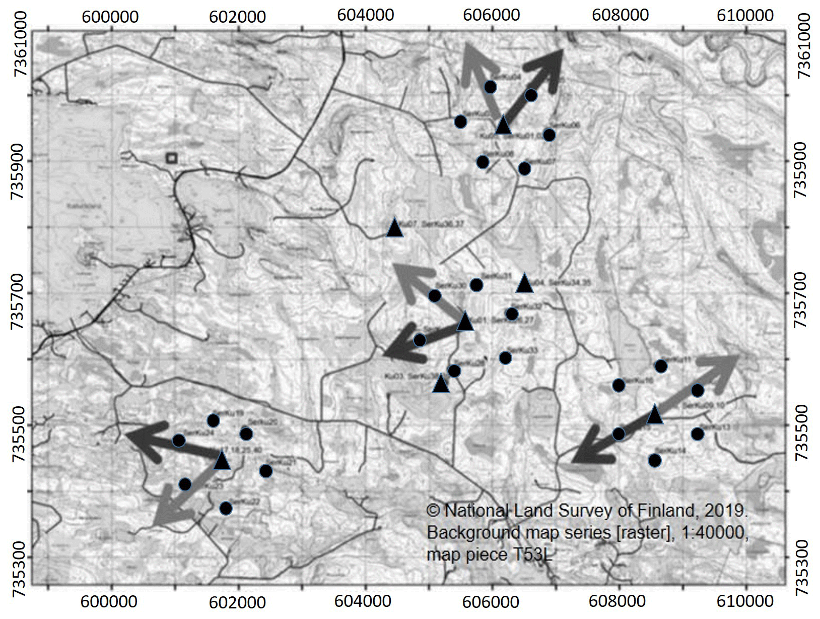
Figure 5Azimuths to main noise sources: dots – stations of the temporary seismic array; black arrows show azimuths to noise sources in the frequency band 10–50 Hz; grey arrows show azimuths to noise sources in the frequency band 5–10 Hz.
In our study, we analyse records of seismic noise with a duration of 10 min for each hour of records. We applied this procedure to records from stations which are the most distant from the mine and located in both parts of the profile (PLB01 and PLB24). We have selected two frequency bands (2–5 and 5–10 Hz) for analysis because they correspond to strong and stable seismic noise, from which it is possible to retrieve surface waves. The result is shown in Fig. 4 as a percentage of record time during which the recorded wave fields approached from certain azimuths with respect to the total time of the record. In Fig. 4, the azimuth of 0∘ corresponds to the true north and shadowed sectors denote the azimuths to the noise sources. Radial sizes of these sectors are proportional to the relative source-acting time calculated as a percentage of the total measurement time while angular sizes of the sectors correspond to errors of the azimuth calculation.
In Fig. 4a, b one can see strong directivity of the noise wave fields from the east. This proves that the main noise source for the eastern part of the profile and for the frequency bands of 2–5 and 5–10 Hz is the mine. Considering the western part of the profile, there is no such clear directivity of the noise wave fields as revealed for the eastern part. One can see a near-homogeneous azimuthal distribution of the noise sources for azimuths between about 250 and 300∘. This could be explained by the location of the profile close to the open pit that occupies a larger area than the underground mine. Because of this, the point-source approximation of noise sources is not valid. From these results we can conclude that if we simply stack all calculated cross-correlation functions for a pair of stations (in particular, in the eastern part of the profile), the final EGF would be biased. Therefore, for the estimation of the EGF with minimum bias, we need to apply the advanced method of stacking described above.
In the second case, we considered the KuGB area with a low level of high-frequency noise. In order to investigate the spatial and azimuthal distribution of the strongest noise sources, we applied the procedure described above to the data of each of the small-aperture arrays. The cross-correlation functions were calculated between the central sensor and the other sensors of the array. Figure 5 presents results of the calculations of the azimuths to the strongest seismic noise sources.
In Fig. 5, one can see that for the different small-aperture arrays there are also different azimuths to the sources in the different frequency bands and the directions to the sources depend on frequency. Taking into account the size of our temporary array (aperture of the large array is 3 km and apertures of each small array are 0.7 km), we can assume that the sources of high-frequency seismic noise are located at distances larger than 0.7 km but less than 3 km from the centres of the small-aperture arrays.
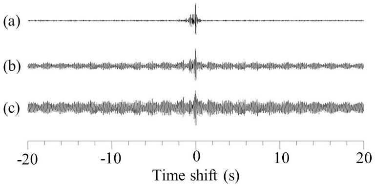
Figure 6Final EGFs (vertical components) calculated by different methods of stacking in the time domain for the frequency band 5–10 Hz: (a) SNR stacking (SNR = 40); (b) weight stacking (SNR = 15.6); (c) rms staking (SNR = 10.4).

Figure 7Build-up process of the EGF from cross-correlation functions by different methods: black dots – by SNR stacking; grey dots – by simple stacking.
For the estimation of EGFs, it is necessary to apply a procedure for data preparation. This procedure includes several steps, such as spectral whitening, removing parts of records with earthquakes, blasts, and missed data. This procedure is applied to the data of both experiments in our study. In the previous parts of our paper, we have demonstrated that the Pyhäsalmi mine is the source of continuous and strong seismic noise in the frequency band of 1–10 Hz. Therefore, we extract EGFs separately for the eastern and western parts of the profile.
Each part of the profile includes one sensor installed in the closest vicinity of the mine, and we calculated cross-correlation functions between those sensors and each of the other sensors in both parts of the profile. Industrial seismic noise may consist of surface and body waves because of different types of noise sources.
There are several methods of stacking the cross-correlation functions in the time domain, for example, the root-mean-square method of Shirzad and Shomali (2015) and the weighted stack by Cheng et al. (2015). We compare the SNR of EGFs estimated by our method for the Pyhäsalmi experiment to the SNR of EGFs estimated by root-mean-square and weighted stacking methods, respectively. The SNR was calculated with respect to the surface wave signal seen in EGFs. Results of this comparison are presented in Fig. 6.
In Fig. 6, one can see that after the application of the SNR-stacking method we obtained the EGF with the highest signal-to-noise ratio of surface waves, compared to the other two methods of stacking. This is because we used only cross-correlation functions coherent with each other in our stacks. As one can see from Fig. 7, the algorithm selects only about 10 % of the total number of cross-correlation functions for the final stack. Nevertheless, it does not mean that there are only few cross-correlation functions coherent with each other. It means that after some iterations the signal-to-noise ratio did not increase any more by adding new functions to the stack. In other words, the algorithm has found a global maximum of the objective function described in Sect. 2.
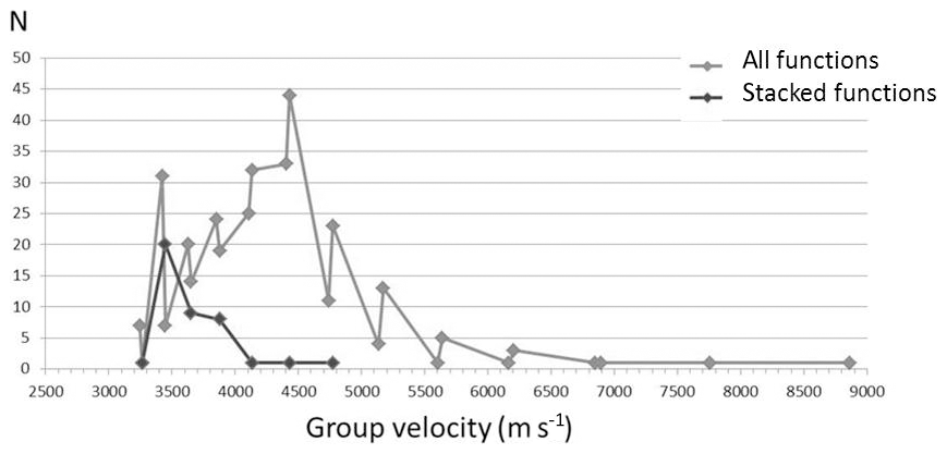
We analysed the apparent velocities obtained from the maxima of each of the cross-correlation functions and the apparent velocities from the cross-correlation functions selected by our algorithm of stacking (Fig. 8). This figure shows that most of the retrieved EGFs have group velocities of about 4500 m s−1. After applying a simple stacking procedure to these cross-correlation functions, the group velocity of the surface wave part of the resulting EGF is about 4500 m s−1. This cannot be true velocity, as it is too high for surface waves propagating in the uppermost bedrock. As can be seen from Fig. 8, our SNR-stacking algorithm has selected only EGFs with group velocity of about 3400 m s−1. This velocity is close to the minimal value from all group velocities, and it is in agreement with group velocities of surface waves and S-wave velocities in the uppermost part of the bedrock in Fennoscandia (Kobranova, 1986; Dortman, 1992; Silvennoinen and Kozlovskaya, 2007; Janik et al., 2009; Poli et al., 2013, etc.). Therefore, after applying our stacking method, we can retrieve EGFs with true group velocity and a maximum SNR.
We apply our method of stacking to the cross-correlation functions calculated for the eastern and western parts of the profile for the frequency bands of 2–5 and 5–10 Hz separately. After stacking, we analysed particle motion diagrams of the waves retrieved from the seismic noise. Figure 9 shows the result of stacking and particle motion analysis of EGFs.
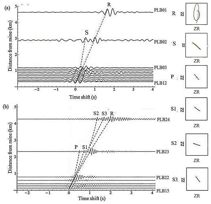
Figure 9Result of stacking and particle analysis of the EGF, evaluated in the Pyhäsalmi experiment: (a) western part of the profile in the frequency band 2–5 Hz; (b) eastern part of the profile in the frequency band 5–10 Hz.
In Fig. 9, we present only EGFs that probably also contain body waves because other EGFs, namely those calculated for the western part in the band of 5–10 Hz and for the eastern part in the band of 2–5 Hz, contain only surface wave parts. Figure 9a shows that the seismic noise recorded in the western part of the profile retrieves mainly Rayleigh waves with group velocity of about 3400 m s−1. The other wave is marked in Fig. 9a as an S wave because the particle motion diagram corresponds to this type of a wave. Nevertheless, this wave has an apparent velocity of 5700 m s−1, which is too high. Therefore, we speculate that this can be an artefact and that phase cannot be used for further analysis. In the frequency band of 5–10 Hz, the EGFs calculated for the eastern part of the profile (Fig. 10b) consist of Rayleigh wave. The other arrivals could correspond to one reflected P wave and three reflected S waves. Apparent velocities of reflected P, S1, S2, and S3 waves are about 4480, 3192, 3261, and 2543 m s−1, respectively. Our assumption that these phases may correspond to retrieved body waves is based solely upon a comparison of their travel times with the travel times of body waves recorded during previous active source experiment in Pyhäsalmi (Heinonen et al., 2012). Alternatively, the extracted waves may correspond to other phases, for example, to direct waves generated by sources inside the mine. Unfortunately, these assumptions cannot be proved using our data, and it would be necessary to use the higher-density array for the precise phase identification of body waves. In our study, the error in velocity estimation is assumed to be equal to a quarter of the wavelength of an extracted signal. The error of the polarization calculation is about 1–3∘.

Figure 10Empirical Green's functions calculated from records of small-aperture arrays in the Kuusamo experiment in the frequency band of 5–10 Hz and stacked (vertical components): (a) by the simple stacking method; (b) by the SNR-stacking method. The EGFs in panels (a) and (b) are sorted according to distance from sensor SK7.
For the KuGB experiment, we calculate cross-correlation functions for each small-aperture array and apply the SNR-stacking algorithm for the EGF evaluation. Cross-correlation functions are calculated between the central sensor and each other sensor of the corresponding small-aperture array. In Fig. 10b, we present results of the EGF calculation by the SNR-stacking method for one of the small-aperture arrays (SK1-SK8 in Fig. 2).
In Fig. 10, one can see that after the application of simple stacking, there are many implicit maxima in the retrieved EGFs. Due to this, it is not possible to calculate the azimuth to noise sources and apparent seismic wave velocities. However, the application of SNR stacking allows the retrieval of the EGFs with maxima corresponding to surface waves propagating from a virtual source with an apparent velocity of about 320–350 m s−1. These waves could be Rayleigh waves or acoustic waves propagating in the air. This assumption is based on the fact that a velocity of 350 m s−1 is close both to the velocity of sound in the atmosphere and to the velocity of surface waves propagating in the shallow quaternary sediments in the uppermost subsurface. For a precise determination of the wave type, it would be necessary to have a more dense observation network. Nevertheless, using our SNR-stacking algorithm we extracted surface waves from the high-frequency seismic noise. As we noticed in the previous section, the noise sources were distributed stochastically, both in space and in time, and the intensity of these noise sources was small. The body waves are not seen in Fig. 10b because a higher density array is necessary for their proper identification.
Classical passive seismic interferometry is based on diffuse-field approximation because of the equivalence of correlation properties of the multiple scattering and resulting wave fields. Therefore, it is possible to evaluate EGFs from averaged cross-correlation functions (Campillo, 2006; Shapiro and Campillo, 2004). In practice, one needs to average over long time intervals (more than 1 year) because of heterogeneous and anisotropic distributions of ambient seismic noise sources during short time intervals (Wapenaar et al., 2010). This is a serious limitation for the practical application of passive seismic interferometry as a method of applied geophysics because it is not always possible to have long-term data acquisition experiments for solving applied problems (mining exploration, microseismic zonation, etc.). In such applied problems, the alternative may be to use ballistic waves, not scattered from heterogeneities but produced by some localized sources of seismic noise (Mulargia, 2012). The major challenge in this case is retrieving body waves from seismic noise. Recently, some techniques of body-wave extraction have been proposed in Vidal et al. (2014) and Panea et al. (2014). The main idea of these techniques is separating ambient seismic noise into a body-wave part and a surface wave part. One could expect that a combination of these separation methods with our technique of stacking would significantly increase the quality of the retrieved body waves. Nevertheless, for this it would be necessary to have the data of dense high-resolution seismic arrays, so making new experiments would be a next step in the development of our technique.
As discussed in the “Introduction” section, there are several methods based on weighted stacking of cross-correlation functions in the time, frequency, and time–frequency domains, which allow us to increase the quality of extracted EGFs (Schimmel et al., 2011; Cheng et al., 2015; Liu et al., 2016; Li et al., 2018, etc.). We showed in previous sections that our time-domain algorithm based on the global optimization of the signal-to-noise ratio makes it possible to exclude incoherent cross-correlation functions from stacking and generally allows obtaining EGFs of even better quality. Of course, it is possible to use the signal-to-noise ratio increase criterion in the frequency or in the time–frequency domains, but this would make the algorithm significantly more complicated. It is necessary to remember, however, that this algorithm can be applied because ambient noise sources are generally characterized by a relatively wide frequency band. In this case one can expect that increasing the signal-to-noise ratio for the dominant frequency would result in an increase in the signal-to-noise ratio of all other frequencies of the signal, as shown in Bensen et al. (2007).
The algorithm proposed in this paper has several limitations and drawbacks and hence has the potential for improvement. Our technique of stacking allows increasing the signal-to-noise ratio, but it has to be applied in combination with array configuration, which allows us to keep control over the azimuthal distribution of noise sources and to guarantee that the stationary phase condition is satisfied. It can be also envisaged that using the mode of noise level distribution instead of the average would make the algorithm more robust with respect to outliers. Another important limitation is the relationship between the time of seismic wave propagation between neighbouring sensors and the dominant period of the retrieved EGFs. If the time of surface wave propagation is about one or two periods of this wave, then it would not be possible to separate body and surface waves, similar to the situation in seismic experiments with active sources. Moreover, the increase in signal-to-noise ratio of one event, for example, a retrieved surface wave, might lead to a decrease in the signal-to-noise ratio of other phases, in particular, body waves.
In certain situations, increasing the SNR after the addition of a new function to the stack is not always achieved due to the coherence of the stacked functions. For example, if the coda wave part in a cross-correlation function gets smaller, then the SNR increases, although stacked functions might not be coherent with each other. The results of testing the algorithm with real data demonstrated, however, that the algorithm is robust and works fine with the high-frequency seismic noise acquired in two completely different areas. The results obtained for the KuGB area demonstrate that the SNR-stacking method might be useful for building up an EGF by stacking ballistic surface wave signals retrieved from the ambient noise. In our study the high quality of surface waves in EGFs was achieved both for brownfield and greenfield exploration areas. Experimental data used in our study are insufficient to make a detailed evaluation of how this technique works with body-wave signals, and it will be the subject of our research in the future.
Results of our study suggest that classical approaches for the EGF evaluation from ambient seismic noise (Campillo, 2006) cannot be considered as a universal tool for extracting high-frequency EGFs. In particular, in quiet areas with a low level of anthropogenic and industrial noise the method would require a long registration time because sources of high-frequency wave fields are weak and their distribution is non-stationary both in space and time. One of the ways to treat the problem is to use ballistic waves and develop and improve methods for the selection of coherent parts of the ambient noise wave field. The study of the azimuthal distribution of ambient noise sources using array techniques is necessary prior to passive seismic experiments, both in greenfield and brownfield exploration areas.
The presented algorithm of cross-correlation function stacking in a time domains allows us to significantly increase the signal-to-noise ratio of retrieved EGFs. In our study we demonstrated that under certain conditions the body waves could be extracted from high-frequency industrial seismic noise using the proposed algorithm. This was illustrated with the data collected during a passive seismic experiment near the Pyhäsalmi underground mine. Nevertheless, for more detailed testing of the possibility of extracting body waves, it would be necessary to analyse the data collected with a higher-density seismic array near the mine.
The presented algorithm of stacking makes it possible to extract EGFs from ambient seismic noise with frequencies higher than 1 Hz recorded in quiet areas without strong sources of industrial noise using 2-D seismic arrays. This has been demonstrated by the application of our technique to the data collected in the Kuusamo Greenstone belt area that is characterized by a low level of anthropogenic seismic noise and has no industrial sites located nearby.
The raw data and processed data of the SEISLAB project are embargoed until 31 December 2019 and will be published in open access after the end of embargo period. Please contact Elena Kozlovskaya (elena.kozlovskaya@oulu.fi) concerning access to the data.
EK and NA have written the majority of the text: introduction, algorithm description, description of results, and discussion conclusions sections; JaN, JoN, and EK planned the experiments in Pyhäsalmi and Kuusamo, organised field work and data acquisition, and performed raw data processing.
The authors declare that they have no conflict of interest.
This article is part of the special issue “Advances in seismic imaging across the scales”. It is not associated with a conference.
Authors thankful to the staff of Sodanlylä Geophysical Observatory of the University of Oulu for assistance in SEISLAB data processing.
The study is a part of the SEISLAB project funded by the European Regional Development Fund (ERDF), the Council of Oulu region (Finland), and the Pyhäsalmi Mine Oy and of the ARCEMIS project funded by the KVANTUM Institute of the University of Oulu. The theoretical part of the study was funded by the Federal Agency of Scientific Organizations (project no. AAAA-A18-118012490072-7) and research mobility grant (no. 31166) by the Academy of Finland.
This paper was edited by Nicholas Rawlinson and reviewed by two anonymous referees.
Afonin, N., Kozlovskaya, E., Kukkonen, I., and DAFNE/FINLAND Working Group: Structure of the Suasselkä postglacial fault in northern Finland obtained by analysis of local events and ambient seismic noise, Solid Earth, 8, 531–544, https://doi.org/10.5194/se-8-531-2017, 2017.
Baig, A., Campillo, M., and Brenguier, F.: Denoising seismic noise cross correlations, J. Geophys. Res., 114, 2156–2202, https://doi.org/10.1029/2008JB006085, 2009.
Barazza, F., Malisan, P., and Carniel, R.: Improvement of H/V technique by rotation of the coordinate system, Commun. Nonlinear Sci., 14, 182–193, 2009.
Bensen, G. D., Ritzwoller, M. H., Barmin, M. P., Levshin, A. L., Lin, F., Moschetti, M. P., and Yang, Y.: Processing seismic ambient noise data to obtain reliable broad-band surface wave dispersion measurements, Geophys. J. Int., 169, 1239–1260, 2007.
Boué, P., Poli, P., Campillo, M. P., and Roux, P.: Reverberations, coda waves and ambient noise: Correlations at the global scale and retrieval of the deep phases, Earth Planet. Sc. Lett., 391, 137–145, https://doi.org/10.1016/j.epsl.2014.01.047, 2014.
Bruneton, M., Pedersen, H. A., Farra, V., Arndt, N. T., Vacher, P., Achauer, U., and Grad, M.: Complex lithospheric structure under the central Baltic Shield from surface wave tomography, J. Geophys. Res.-Sol. Ea., 109, B10303, https://doi.org/10.1029/2003JB002947, 2004.
Campillo, M.: Phase and correlation of “random” seismic fields and the reconstruction of the Green function, Pure Applied Geophysics, 163, 475–502, https://doi.org/10.1007/s00024-005-0032-8, 2006.
Cheng, F., Xia, J., Xu, Y., Xu, Z., and Pan, Y.: A new passive seismic method based on seismic interferometry and multichannel analysis of surface waves, J. Appl. Geophys., 117, 126–135, 2015.
Dortman, N. B.: Petrophysics. A Handbook, Book 1, Rocks and Minerals, Nedra, Moscow, 1992.
Douze, E. J. and Laster, S. J.: Statistics of semblance, Geophysics, 44, 1999–2003, https://doi.org/10.1190/1.1440953, 1979.
Groos, J. C., Bussat, S., and Ritter, J. R. R.: Performance of different processing schemes in seismic noise cross-correlations, Geophys. J. Int., 188, 498–512, 2012.
Heinonen, S., Imaña, M., Snyder, D. B., Kukkonen, I. T., and Heikkinen, P. J.: Seismic reflection profiling of the Pyhäsalmi VHMS-deposit: A complementary approach to the deep base metal exploration in Finland, Geophysics, 77, WC15–WC23, 2012.
Janik, T., Kozlovskaya, E., Heikkinen, P., Yliniemi, J., and Silvennoinen, H.: Evidence for preservation of crustal root beneath the Proterozoic Lapland-Kola orogen (northern Fennoscandian shield) derived from P and S wave velocity models of POLAR and HUKKA wide-angle reflection and refraction profiles and FIRE4 reflection transect, J. Geophys. Res.-Sol. Ea., 114, B06308, https://doi.org/10.1029/2008JB005689, 2009.
Kobranova, W. N.: Petrophysics, Nedra, Moscow, 1986.
Kukkonen, I., Heikkinen, P., Elo, S., Heinonen, S.,Laitinen, J., and HIRE Working Group of the Geological Survey of Finland: HIRE Seismic Reflection Survey in the Kemi Cr mining area, northern Finland, Report Q23/2009/64, 2009.
Lehtonen, M. and O'Brien, H.: Mantle transect of the Karelian Craton from margin to core based on PT data from garnet and clinopyroxene xenocrysts in kimberlites, Bulletin of Geological Society of Finland, 81, 79–102, 2009.
Li, G., Niu, F., Yang, Y., and Xie, J.: An investigation of time–frequency domain phase-weighted stacking and its application to phase-velocity extraction from ambient noise's empirical Green's functions, Geophys. J. Int., 212, 1143–1156, 2018.
Liu, X., Ben-Zion, Y., and Zigone, D.: Frequency domain analysis of errors in cross-correlations of ambient seismic noise, Geophysical Supplements to the Monthly Notices of the Royal Astronomical Society, 207, 1630–1652, 2016.
Malehmir, A., Durrheim, R., Bellefleur, G., Urosevic, M., Juhlin, C., White, D. J., Milkereit, B., and Campbell, G.: Seismic methods in mineral exploration and mine planning: A general overview of past and present case histories and a look into the future, Geophysics, 77, WC173–WC190, 2012.
Mulargia, F.: The seismic noise wavefield is not diffuse, J. Acoust. Soc. Am., 131, 2853–2858, 2012.
Nakamura, Y.: A method for dynamic characteristics estimation of subsurface using microtremor on the ground surface, QR Railway Tech. Res. Inst., 30, 25–33, 1989.
Nakata, N., Chang, J. P., Lawrence, J. F., and Boué, P.: Body wave extraction and tomography at Long Beach, California, with ambient-noise interferometry, J. Geophys. Res.-Sol. Ea., 120, 1159–1173, 2015.
Neidell, N. and Turhan Taner, M.: Semblance and other coherency measures for multichannel data, Geophysics, 36, 482–497, 1971.
Panea, I., Draganov, D., Almagro Vidal, C., and Mocanu, V.: Retrieval of reflections from ambient noise recorded in the Mizil area, Romania, Geophysics, 79, Q31–Q42, 2014.
Pedersen, H. A., Debayle, E., Maupin, V., and POLENET/LAPNET Working Group: Strong lateral variations of lithospheric mantle beneath cratons – example from the Baltic Shield, Earth Planet. Sc. Lett., 383, 164–172, 2013.
Place, J. A. P., Malehmir, A., Högdahl, K., Juhlin, C., and Persson Nilsson, K.: Seismic characterization of the Grängesberg iron deposit and its mining-induced structures, central Sweden: Interpretation, 3, SY41–SY56, https://doi.org/10.1190/INT-2014-0212.1, 2015.
Poli, P., Pedersen, H. A., Campillo, M., and the POLENET/LAPNET Working Group: Emergence of body waves from cross-correlation of short period seismic noise, Geophys. J. Int., 188, 549–588, 2012a.
Poli, P., Pedersen, H., Campillo, M., and LAPNET Working Group: Body-wave imaging of Earth's mantle discontinuities from ambient seismic noise, Science, 338, 1063–1065, https://doi.org/10.1126/science.1228194, 2012b.
Poli, P., Campillo, M., Pedersen, H., and the POLENET/LAPNET Working Group: Noise directivity and group velocity tomography in a region with small velocity contrasts: the northern Baltic shield application to the northern Baltic Shield, Geophys. J. Int., 192, 413–424, https://doi.org/10.1093/gji/ggs034, 2013.
Phạm, T.-S., Tkalčić, H., Sambridge, M., and Kennett, B. L. N.: Earth's correlation wavefield: Late coda correlation, Geophys. Res. Lett., 45, 3035–3042, https://doi.org/10.1002/2018GL077244, 2018.
Rost, S. and Thomas, C.: Array seismology: methods and applications, Rev. Geophys., 40, 2-1–2-27, https://doi.org/10.1029/2000RG000100, 2002.
Sambridge, M.: Geophysical inversion with a neighbourhood algorithm – I. Searching a parameter space, Geophys. J. Int., 138, 479–494, 1999.
Schimmel, M., Stitsmann, E., and Gallart, J.: Using instantaneous phase coherence for signal extraction from ambient noise data at a local to a global scale, Geophys. J. Int., 184, 494–506, 2011.
Schweitzer, J., Fyen, J., Mykkeltveit, S., Gibbons, S. J., Pirli, M., Kühn, D., and Kværna, T.: Seismic Arrays in New Manual of Seismological Observatory Practice (NMSOP-2), German Research Centre for Geosciences, ISBN 3-9808780-0-7.9, 1–80, 2012.
Shapiro, N. M. and Campillo, M.: Emergence of broadband Rayleigh waves from correlations of the ambient seismic noise, Geophys. Res. Lett., 31, L07614, https://doi.org/10.1029/2004GL019491, 2004.
Shapiro, N. M., Campillo, M., Stehly, L., and Ritzwoller, M. H.: High-Resolution Surface-Wave tomography from ambient seismic noise, Science, 307, 1615–1618, 2005.
Shirzad, T. and Shomali, Z. H.: Extracting seismic body and Rayleigh waves from the ambient seismic noise using the rms-stacking method, Seismol. Res. Lett., 86, 173–180, 2015.
Silvennoinen, A.: Kuusamon ja Rukatunturin kartta-alueiden kalliopera – Espoo, Geological Survey of Finland, Espoo, Finland, 1991.
Silvennoinen, H. and Kozlovskaya, E.: 3D structure and physical properties of the Kuhmo Greenstone Belt (eastern Finland): Constraints from gravity modelling and seismic data and implications for the tectonic setting, J. Geodyn., 43, 358–373, 2007.
Silvennoinen, H., Kozlovskaya, E., Kissling, E., Kosarev, G., and POLENET/LAPNET working group: A new Moho boundary map for the northern Fennoscandian Shield based on combined controlled-source seismic and receiver function data, GeoResJ, 1, 19–32, 2014.
Tiira, T., Janik, T., Kozlovskaya, E., Grad, M., Korja, A., Komminaho, K., and Brückl, E.: Crustal Architecture of the Inverted Central Lapland Rift along the HUKKA 2007 Profile, Pure Appl. Geophys., 171, 1129–1152, 2014.
Ventosa, S., Schimmel, M., and Stutzmann, E.: Extracting surface waves, hum and normal modes: time-scale phase-weighted stack and beyond, Geophys. J. Int., 211, 30–44, https://doi.org/10.1093/gji/ggx284, 2017.
Vidal, C. A., Draganov, D., Van der Neut, J., Drijkoningen, G., and Wapenaar, K.: Retrieval of reflections from ambient noise using illumination diagnosis, Geophys. J. Int., 198, 1572–1584, 2014.
Vinnik, L., Oreshin, S., Makeyeva, L., Peregoudov, D., Kozlovskaya, E., Pedersen, H., and Jämsen, T.: Anisotropic lithosphere under the Fennoscandian shield from P receiver functions and SKS waveforms of the POLENET/LAPNET array, Tectonophysics, 628, 45–54, 2014.
Wapenaar, K., Draganov, D., and Robertsson, J. (Eds.): Seismic interferometry: History and present status, Society of Exploration Geophysicists, Geophysics Reprint Series No. 26, ISBN 978-1-56080-150-4, 2008.
Wapenaar, K., Draganov, D., Snieder, R., Campman, X., and Verdel, A.: Tutorial on seismic interferometry: Part 1 – Basic principles and applications, Geophysics, 75, 75A195, https://doi.org/10.1190/1.3457445, 2010.
Weihed, P., Arndt, N., Billström, K., Duchesne, J.-C., Eilu, P., Martinsson, O., Papunen, H., and Lahtinen, R.: Precambrian geodynamics and ore formation: The Fennoscandian Shield, Ore Geol. Rev., 27, 273–322, https://doi.org/10.1016/j.oregeorev.2005.07.008, 2005.
Yliniemi, J., Kozlovskaya, E., Hjelt, S. E., Komminaho, K., Ushakov, A., and SVEKALAPKO Seismic Tomography Working Group: Structure of the crust and uppermost mantle beneath southern Finland revealed by analysis of local events registered by the SVEKALAPKO seismic array, Tectonophysics, 394, 41–67, 2004.
- Abstract
- Introduction
- Advanced technique of cross-correlation function stacking
- Experimental data
- Analysis of the seismic noise
- Empirical Green's functions estimation
- Discussion
- Conclusion
- Data availability
- Author contributions
- Competing interests
- Special issue statement
- Acknowledgements
- Financial support
- Review statement
- References