Subsurface characterization of a quick-clay vulnerable area using near-surface geophysics and hydrological modelling

Quick-clay landslides are common geohazards in Nordic countries and Canada. The presence of potential quick clays is confirmed using geotechnical investigations, but near-surface geophysical methods, such as seismic and resistivity surveys, can also help identify coarse-grained materials associated with the development of quick clays. We present the results of reflection seismic investigations on land and in part of the Göta River in Sweden, along which many quick-clay landslide scars exist. This is the first time that such a large-scale reflection seismic investigation has been carried out to study the subsurface structures associated with quick-clay landslides. The results also show a reasonable correlation with radio magnetotelluric and travel-time tomography models of the subsurface. Other ground geophysical data, such as high magnetic values, suggest a positive correlation with an increased thickness of the coarse-grained layer and shallower depths to the top of the bedrock and the top of the coarse-grained layer. The morphology of the river bottom and riverbanks, e.g. subaquatic landslide deposits, is shown by side-scan sonar and bathymetric data. Undulating bedrock, covered by subhorizontal sedimentary glacial and postglacial deposits, is clearly revealed. An extensive coarse-grained layer (P-wave velocity mostly between 1500 and 2500 m s⁻¹ and resistivity from approximately 80 to 100 Ωm) exists within the sediments and is interpreted and modelled in a regional context. Several fracture zones are identified within the bedrock. Hydrological modelling of the coarse-grained layer confirms its potential for transporting fresh water infiltrated in fractures and nearby outcrops located in the central part of the study area. The modelled groundwater flow in this layer promotes the leaching of marine salts from the overlying clays by seasonal inflow–outflow cycles and/or diffusion, which contributes to the formation of potential quick clays.

1 Introduction

Quick clays are sensitive glacial and postglacial sediments, mostly deposited in a shallow-water marine environment, whose structure can collapse and liquefy if disturbed (Osterman, 1963; Torrance, 2012). These sediments were deposited in the last deglaciation and early postglacial and subsequently isostatically raised above sea level (Torrance, 2012). Due to the infiltration of meteoric waters, mineral salts were leached out, which changed the salinity of the pore water and altered their soil properties (Rosenqvist, 1953). The leaching of salts is important in the development of characteristic quickness behaviour (Rosenqvist, 1946; Torrance, 2012), but there are other factors that influence the formation of quick clays, such as the presence of dispersing agents and pH level (Salas-Romero et al., 2016; Torrance, 2012). The presence of quick clays can only be confirmed using geotechnical site and laboratory investigations enabling the estimation of the sensitivity (Rankka et al., 2004). The sensitivity is defined as the ratio of undrained undisturbed to remoulded shear strength. In Sweden, where this work is focused, quick clays are defined as clays with a sensitivity higher than 50 and a remoulded shear strength of less than 0.4 kPa (Karlsson and Hansbo, 1989).

Quick-clay landslides are common in northern countries such as Sweden, Norway, and Canada. They are also known worldwide due to catastrophes such as in Rissa (Gregersen, 1981), Tuve (Larsson and Jansson, 1982), and Saint-Jude (Locat et al., 2017), and they have been studied in different fields of geoscience (Dahlin et al., 2013; Lundström et al., 2009; Salas-Romero et al., 2016; Sauvin et al., 2014; Solberg et al., 2016; Wang et al., 2016). In order to define areas susceptible to quick-clay landslides in Sweden, Rankka et al. (2004) reviewed a number of geological and geohydrological prerequisites for the formation of quick clay. This list includes glaciomarine sediments, thin clay deposits, underlying coarse-grained layers, peaks in the bedrock surface that retain accumulating groundwater, artesian groundwater pressure, highly permeable layers within the clay deposits, height above sea level, organic soils, a large catchment area, and infiltration from more than one direction. The triggering of quick-clay landslides is influenced by natural conditions (heavy rainfall, high–low water flow along the river, river erosion, or variation of the groundwater level) and by human activities (construction or loading–unloading works) (Thakur et al., 2014). With a minimal slope angle and a place to flow to, any mechanism that increases stress on the quick clays or reduces their strength may trigger a landslide. In Sweden, model scenarios for climate change over the next 100 years predict warmer and wetter conditions (Swedish Government Official Reports, 2007), which means more precipitation in the west of the country, more runoff water, and higher river discharge, increasing the likelihood of landslides in areas that are already prone to them. More variability in river level, as predicted by climate studies (Swedish Government Official Reports, 2007), may destabilize some slopes along the shores, causing new landslides.

The Göta River valley, which is located in southwest Sweden, hosts many landslide scars, most of which are quick-clay related (Swedish Geotechnical Institute – SGI, 2012a). The valley is filled with thick marine postglacial deposits that overlie undulating bedrock (SGI, 2012a). The Göta River is one of the longest rivers in Sweden (93 km long), the source of drinking water for more than 700 000 people, a transport route, and the main outflow of the country's largest lake, Vänern (SGI, 2012a). One or more large landslides could dam the river, affecting river-based transportation with economic and social consequences. In June of 1957 a landslide took place at the sulfite factory located next to the Göta River (in the southern part of the municipality of Lilla Edet). This landslide, one of the biggest to have been observed in Sweden, caused a lot of structural damage (Fig. 1) and the loss of three lives. The landslide propagated backwards in a retrogressive manner and along the riverbank, transporting large amounts of materials into the river, triggering a wave of 5 to 8 m in height and covering around 32 ha (Hultén et al., 2006; Odenstad, 1958). It has been suggested that the landslide was triggered by the infiltration of sulfite liquor and other chemicals into the ground, which reduced the clay shear strength, in combination with other factors such as erosion at the riverbank and the presence of quick clay (Odenstad, 1958).

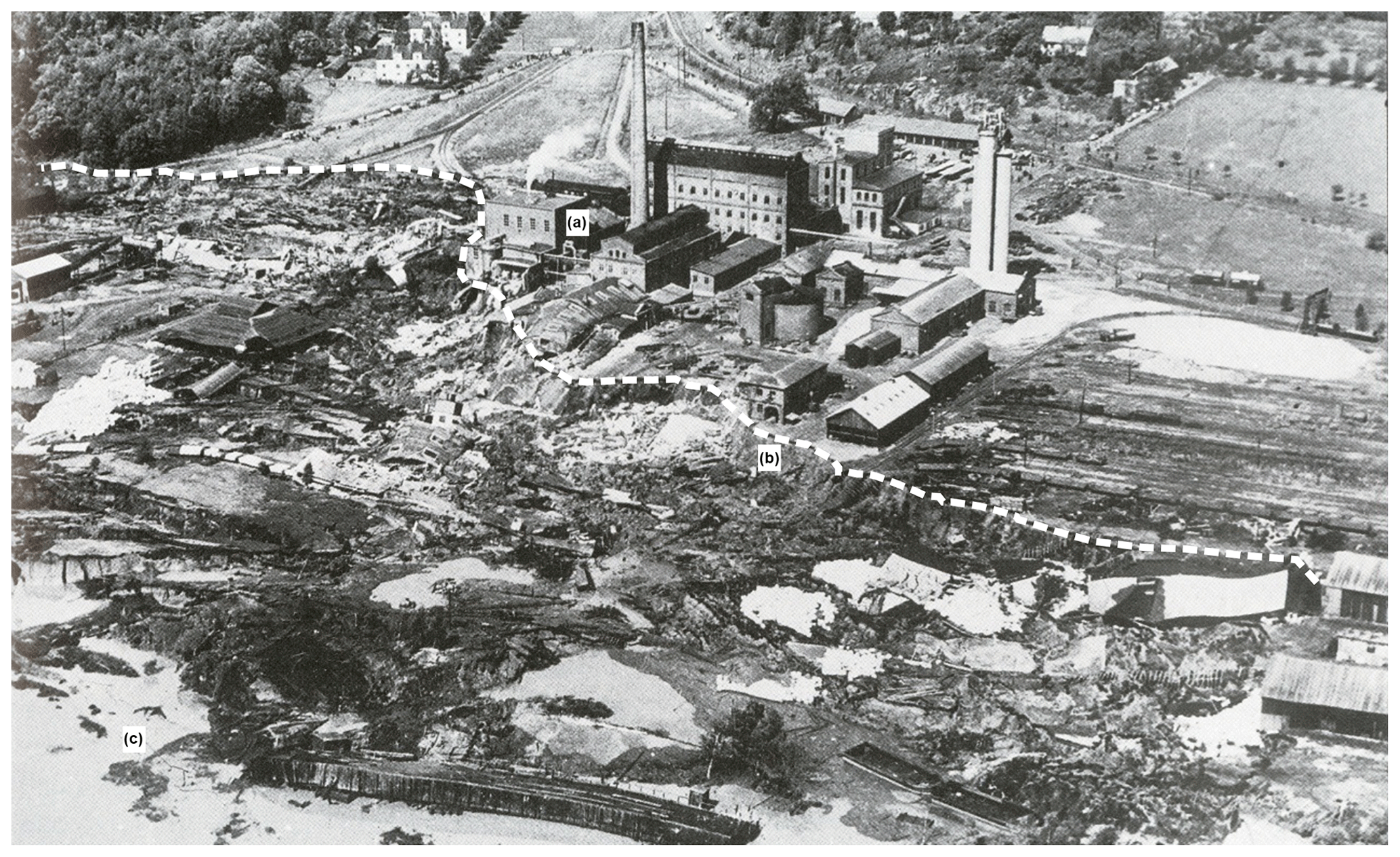
Figure 1 Aerial photo from the 1957 Göta landslide. The picture shows the sulfite factory located next to the river where the landslide started. (a) Factory, (b) slide back wall, and (c) river. Photo: Edet group's archive.

This study is based on a joint interpretation of multidisciplinary datasets for testing whether an area close to the centre of Lilla Edet is susceptible to quick-clay landslides using the prerequisites described by Rankka et al. (2004), focusing on building a hydrogeological model that may represent the study area. The detailed objectives are (i) 3-D geological–geophysical modelling of the larger-scale subsurface structures overlying and existing within bedrock-like possible fracture zones, (ii) understanding the role of an identified coarse-grained layer and its spatial relationship with the bedrock surface that may improve the hazard assessment, (iii) hydrological modelling of the groundwater within the coarse-grained layer to better understand the development of quick clays in the study area, and (iv) investigating the riverbanks of the Göta River, its bed, and mass-movement deposits. Reflection seismic (both legacy and new sets of seismic profiles acquired within this study), P-wave refraction tomography (mainly from Wang et al., 2016, but for the new profiles performed in this study), and airborne transient electromagnetic (ATEM) and radio magnetotelluric (RMT) resistivity models (Bastani et al., 2017; Wang et al., 2016) are correlated with borehole data (Branschens Geotekniska Arkiv – BGA, 2018; Salas-Romero et al., 2016) for the identification of different types of clays, coarse-grained materials, and bedrock. Using the interpreted seismic sections together with total sounding (BGA, 2018) and high-resolution lidar data (©Lantmäteriet), elevation surfaces from the top of the bedrock and the top and bottom of the coarse-grained layer are modelled. This study demonstrates not only that this layer covers a larger area than initially thought (earlier studies showed the local extension of this layer), but also confirms its hydrological potential as a transport path for infiltrating fresh water from nearby outcrops and fractures. Surface magnetic data serve to illustrate that the coarse-grained layer together with quick clays may have acted as a sliding surface at a landslide scar located within the survey area. Other datasets, such as side-scan sonar and bathymetry, are also analysed to investigate the riverbed and its influence on the development of quick-clay landslides. This work provides a good example of the integration of a large amount of different types of data for the study of an area prone to quick-clay landslides.

2 Study area

The work presented in this paper is a continuation of previous studies conducted in an area prone to quick-clay landslides in southwest Sweden in 2011 and 2013 (Malehmir et al., 2013a; Salas-Romero et al., 2016). The study area is within the municipality of Lilla Edet in a region called Fråstad, which the Göta River crosses. Lilla Edet has around 14 000 inhabitants (Lilla Edets Kommun, 2018) and is located approximately 8 km south of this area, on the eastern side of the river. The geology of the study area consists mostly of gentle reliefs of glacial and postglacial deposits such as clay, silt, and sand, with some granite to granodiorite bedrock outcrops (©Geological Survey of Sweden – SGU, Fig. 2a). Along the shorelines, landslide scars can be found. Precisely at the survey site several landslide scars are visible along both sides of the river, one of them located in the middle of the survey area (Fig. 2a–b). A net of morphological lineaments, mostly fracture zones, covers most of the area represented in Fig. 2a. Among these lineaments, one of the prominent ones follows the river profile and another one has an E–W direction. It is known that the bedrock in the Göta River valley has an extended system of cracks, with a fault zone that follows the river channel (SGI, 2012b). Figure 2b shows high-resolution lidar data (©Lantmäteriet) ranging from 7 to 97 m of elevation. Two of the seismic profiles acquired in this study, lines 6 and 7, are located in an area with lower elevation compared to the rest of the land seismic lines. In this area a large landslide scar is visible (Fig. 2a–b) and shows a horst and graben pattern, classifying this landslide as a spread type (Demers et al., 2017).

Figure 2 Quick-clay study site location. (a) Geological map of the study area (©SGU), Fråstad, in southwest Sweden. Shot positions SH5 and SH7 (black and white stars) from line 5–5b and line 7, respectively. (b) Lidar elevation map of the study area (©Lantmäteriet). (c) Sketch of the Göta River that includes the position of the study area (b) and the position of figures shown later in the paper. The red arrows in (c) indicate the beginning and end of the river seismic lines.

Previous studies included P- and S-wave reflection and refraction surveys, potential fields, controlled-source tensor (CSTMT) and RMT, electric resistivity tomography (ERT), and ground-penetrating radar (GPR). In 2013 three boreholes (BH1 to BH3 in Fig. 2a–b) were made in the study area, primarily to ground truth geophysical interpretations but also to collect undisturbed core samples for laboratory measurements. Geophysical, geotechnical, and borehole data showed that a coarse-grained layer underlies leached clays (potential quick clays) and quick clays in some places within the study area. The studies suggested that this layer plays a role in leaching the marine salts from the overlying clays and speeds up the formation of quick clays. Some geotechnical investigations (Löfroth et al., 2011) showed that an increased thickness of the coarse-grained layer is correlated with an increased thickness of the quick clays. The sediments above the coarse-grained layer are intercalating layers of silt and clay, and below they are mostly marine clays that extend down to the bedrock. The studies also suggested that the eastern part of the study area has a higher proportion of leached clays than the western part.

3 Data acquisition

3.1 Land reflection seismic profiles

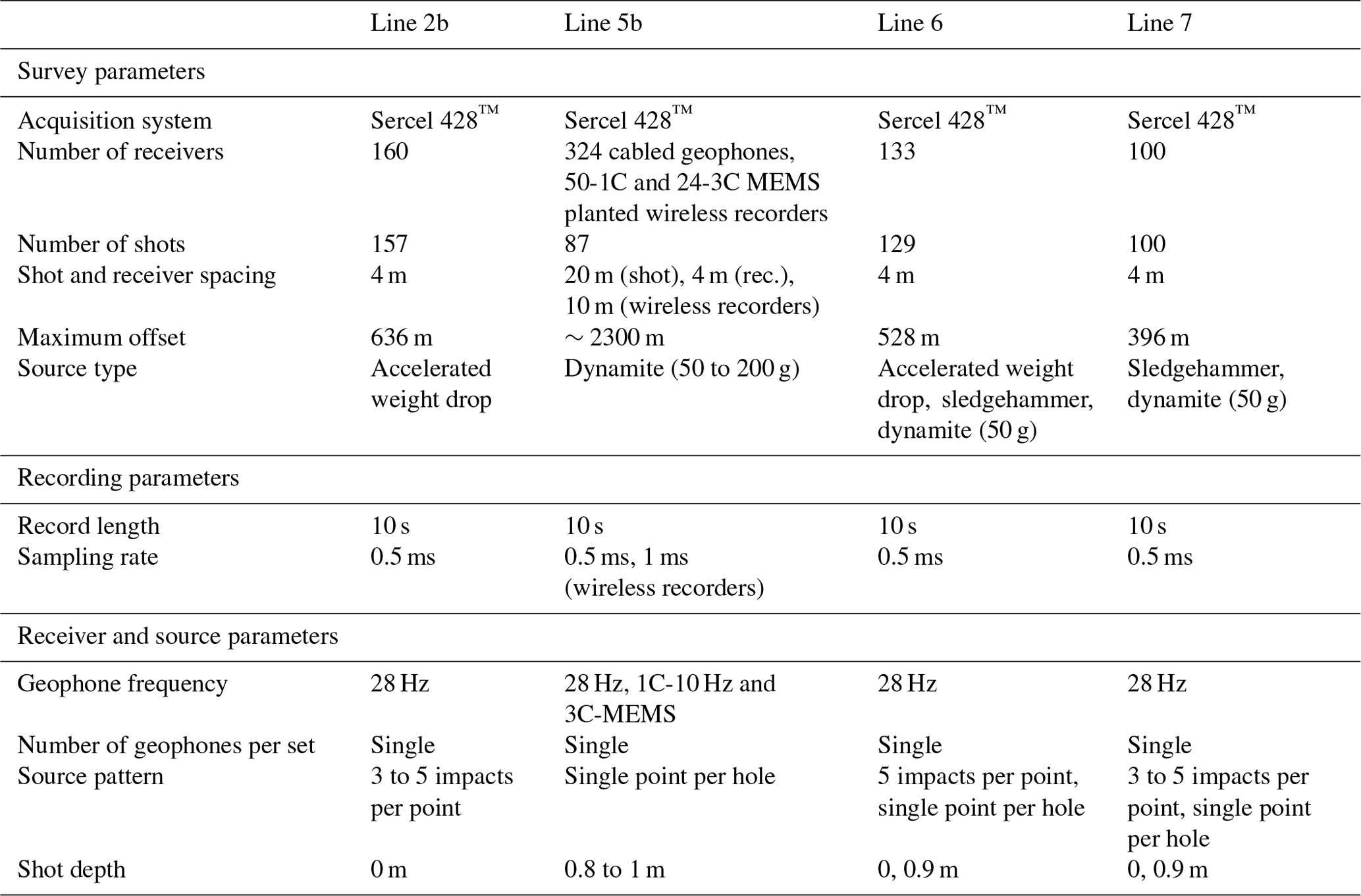
Four land reflection seismic profiles were acquired (this study) during 2 weeks in 2013 (lines 2b, 5b, 6, and 7 in Fig. 2a–b), totalling a length of approximately 3.8 km, aiming to complement existing reflection seismic data (Lundberg et al., 2014; Malehmir et al., 2013a, b) and to obtain an overall understanding of the larger-scale structures. The new lines extend the study area along the N–S direction as line 5b crossed to the northern side of the river. Table 1 compiles the main acquisition parameters. In three of the lines, 2b, 6, and 7, the geophone and shot spacing were the same (4 m), while in the longest line, 5b, they were different. In the southern part of line 5b cabled geophones of 28 Hz were used every 4 m, and in the northern part wireless stations were deployed every 10 m, alternating single-component (1C) receivers of 10 Hz and three-component (3C) broadband digital MEMS (micro-electro-mechanical systems) sensors. Due to the great length of line 5b (∼2300 m), dynamite was used as the source energy and fired at every 20 m in order to obtain high-quality data. In line 2b an accelerated weight drop was used, and in lines 6 and 7 a sledgehammer was the main seismic source because the accelerated weight drop experienced technical problems. At the beginning and at the end of lines 6 and 7, extra shots were made using dynamite. These two lines were connected to each other during the survey, which allowed for simultaneous data acquisition along both lines. Due to the large distance between them (∼300 m) the initial idea of a joint 3-D first-break tomography to resolve the bedrock surface was not possible; nevertheless, individual results were obtained for each line (Wang et al., 2016). The acquisition system was Sercel 428^™, and the survey coordinates were obtained using a differential global positioning system (DGPS) with high-precision geodetic data. The ranges of lateral and vertical nominal resolutions for this method are shown in Table 2. The shown lateral nominal resolution for the reflection seismic data has been obtained by calculating the first Fresnel zone at 20 m of depth.

Table 1 Main acquisition parameters of the seismic lines acquired in this study during March 2013.

3.2 River reflection seismic profiles

Reflection seismic data along the Göta River were acquired from the survey vessel SV Ocean Surveyor (property of SGU) in 2000 and were made available as raw shot records. Two types of acquisition were registered: single-channel (3.5 kHz echo sounder) and six-channel (Fig. 2a–c). Both lines have a similar length (around 16.9 km) and run parallel, with their initial and final points very close to each other (they are shifted with respect to each other by approximately 11 m). In the single-channel line the receiver and shot positions were the same (the average distance between consecutive points is 3 m). In the six-channel line the distance between the source and the nearest receiver is 6 m (maximum offset is 21 m), the receiver spacing being 3 m. A 10 in³ (164 cm³) sleeve gun was used as a source. The frequency range is between 100 and 1000 Hz. Table 2 shows the lateral and vertical nominal resolutions for this method, which have been calculated following the same procedure as in the land reflection seismic data.

Table 2 Nominal resolution (lateral – L and vertical – V) and spatial sampling (SS) of each method.

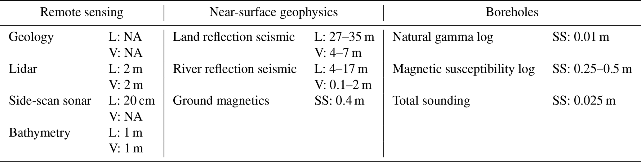
NA – not available.

3.3 Magnetics

The ground magnetic data were collected by Uppsala University during the field campaign of 2011 (Malehmir et al., 2013a). The purpose of this survey was to delineate the bedrock topography by estimating the changes in the magnetic field generated by the rock magnetism. The total-field magnetic and vertical gradient were measured using a walking-mode GPS-mounted magnetometer during 5 d. During the first 3 d a N–S direction was followed, and during the last 2 d an almost E–W direction was followed. In total, 17 128 points were surveyed (see spatial sampling in Table 2). A base station was used for correcting the diurnal variations and instrumental drift. The position of this base station changed along the 5 d, with the biggest difference between the first and the rest of the days (around 53 m). The vertical gradient data did not provide convincing results and were thus disregarded for detailed studies.

3.4 Side-scan sonar and bathymetry

The side-scan sonar data on the Göta River were acquired by SGU in 2000 and were available as a 2-D georeferenced image file (see Table 2). A Klein System of 500 kHz was used. These data are obtained by transmitting sound waves, which are then reflected from underwater elements and provide an acoustic image of the materials and morphology of the riverbed (Kaeser et al., 2013). The amplitude values of the image are represented with a greyscale that indicates the strength of the reflectivity. Normally, dark areas are considered coarse and dense materials like rock boulders or gravel, and light areas are considered fine materials like clays or sand. However, the colour tone can be affected by more factors such as the angle of incidence, water density, and turbulence. The side-scan sonar data cover most of the river shown in Fig. 2a–b and extending a bit further to the south.

Marin Miljöanalys AB collected the bathymetric data using multi-beam echo sounding (Kongsberg EM3002-D, 300 kHz) in 2009 under the assignment of SGI (Marin Miljöanalys AB, 2009). The goal was to create a high-resolution topography model of the riverbed. The data were available as a georeferenced file (see nominal resolution in Table 2).

3.5 Lidar

The lidar scan was collected by Lantmäteriet in 2011. The survey was made from a height of 2000 m, and the average point density is from 0.5 to 1 points m⁻² (see nominal resolution in Table 2).

4 Reflection seismic processing

Table S1 in the Supplement presents the detailed processing steps for the land and river reflection seismic data. The processing of the land reflection seismic data was similar for lines 2–2b, 6, and 7. The preparation of the data required zero-time correction, vertical stacking of repeated shot records, and merging of the new line 2b with the 2011 line 2 (Malehmir et al., 2013b). The removal of first arrivals using a carefully designed top mute filter using picked first breaks and the application of stretch mute (Schmelzbach et al., 2005) helped to enhance the reflections at the shallow parts and avoid misinterpretation of the first arrivals. Refraction static corrections did not give satisfactory results for any of the lines, and they were not applied further. Elevation static corrections were, however, applied using the highest-elevation datum and a velocity of 1500 m s⁻¹. As the data still looked noisy and with lower resolution, more preprocessing steps were necessary. Deconvolution before stacking helped to obtain a reasonably clear seismic section. A series of constant velocity stacks (from 800 to 4000 m s⁻¹) was used in order to obtain the most coherent bedrock reflections. For lines 2–2b, 6, and 7 we used 1400 m s⁻¹ in the first 150 m of depth and 1800 m s⁻¹ from 150 m of depth to the end of the section. A post-stack f–k filter and surface-consistent residual static corrections were applied for data along lines 6 and 7 to improve the continuity of the reflections. Black et al. (1994) show that the migration process is not really necessary for near-surface seismic imaging applications although it can reduce the noise level. After a series of tests, we eventually concluded that migration did not lead to any improvement because the reflections are mostly subhorizontal or gently dipping.

Figure 3 shows an example of a shot record from line 7 (SH7; see the position in Fig. 2a). Figure 3a presents the raw shot gather with only trace balance applied, and Fig. 3b presents the preprocessed shot gather after elevation static corrections, Wiener deconvolution, band-pass filtering, trace editing, the removal of first breaks, and trace balance. The bedrock reflection, B1, is already visible in the raw data but improved in the preprocessed shot record.

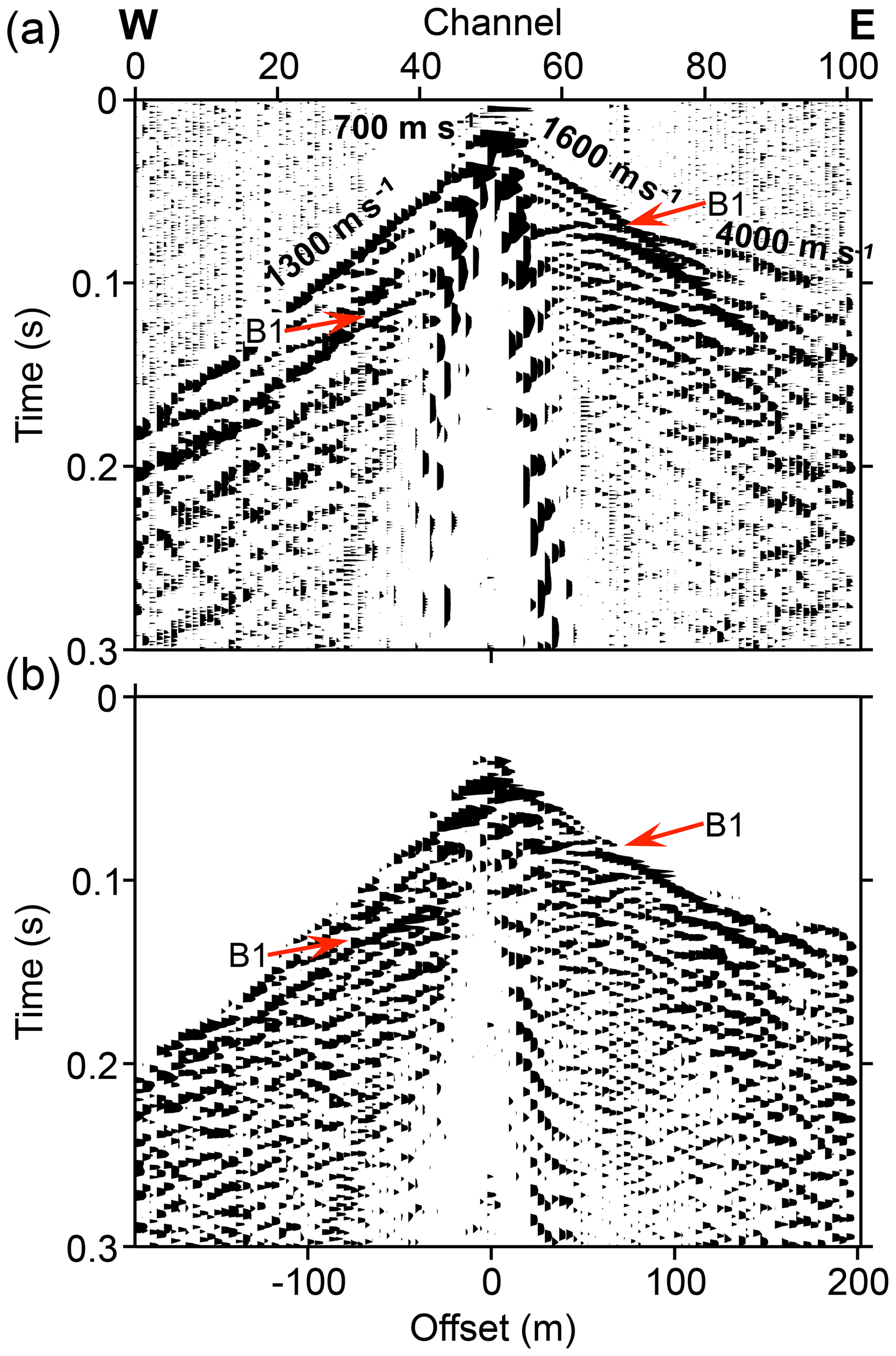
Figure 3 An example of a shot record along line 7 (see SH7 in Fig. 2a). (a) Raw shot gather. Apparent velocities for different types of arrivals are shown at the top of each event. (b) The reflection B1 becomes clearer after a series of pre-stack processing steps. Scale 3H : 4V.

The processing of the land reflection seismic data for line 5–5b was slightly different from the rest of the lines. First, the wireless data needed to be resampled from 1 to 0.5 ms to be consistent with the cabled geophone data. Then, the cabled geophone, 1C, and 3C wireless (vertical component) data were merged. Once all the data were joined, a delay of around 1 s between the cabled geophone and the wireless part was observed (the wireless data were shifted up 1 s). With the data zero-time-shifted, the next step was to merge them with those from the 2011 line 5 (Malehmir et al., 2013b). As the receiver distance was different for the cabled geophone and the wireless parts, it was necessary to process each part separately, applying different geometries for each case (common depth point, CDP, spacing equal to 2 m in the south and 10 m in the north). Before velocity analysis, the processing of both parts included elevation static corrections, the removal of first arrivals using a top mute filter (surgical mute for the wireless data), band-pass filtering, spectral whitening, and f–k filtering for the wireless data. The high-quality data for line 5–5b allowed for a relatively simple processing flow, wherein the velocity analysis greatly improved the result of the final seismic section (performed at 10–20 m of lateral spacing in the southern part; in the northern part constant velocities, from 800 to 4000 m s⁻¹, were tested). The velocity analysis of the wireless seismic data revealed that the deeper part of the section needed higher velocities to obtain visually coherent reflections, and thus the data were divided in two parts for processing: from 0 to 80 ms (using a velocity of 1300 m s⁻¹) and from 80 to 500 ms (using a velocity of 3100 m s⁻¹). The post-stack processing included band-pass filtering for both types of data (cabled geophone and wireless) and post-stack deconvolution in the case of the wireless data.

Figure 4 shows an example of a shot record along line 5–5b (SH5; see the position in Fig. 2a). Figure 4a is the raw shot gather, and Fig. 4b is the preprocessed shot gather (elevation static corrections, band-pass filtering, spectral whitening, trace editing, the removal of first breaks, and automatic gain control – AGC). In Fig. 4b a number of reflections seem to be revealed: bedrock reflection B1 and a shallower one from the top of the coarse-grained layer S1. The sediments show P-wave velocities ranging from 1000 to 2000 m s⁻¹, while the bedrock shows velocities much higher than 3000 m s⁻¹ (Wang et al., 2016). The values are similar to those in line 7 (Fig. 3a), except for the direct wave, which is much slower in that case. It may be related to near-surface effects or differences in topography.

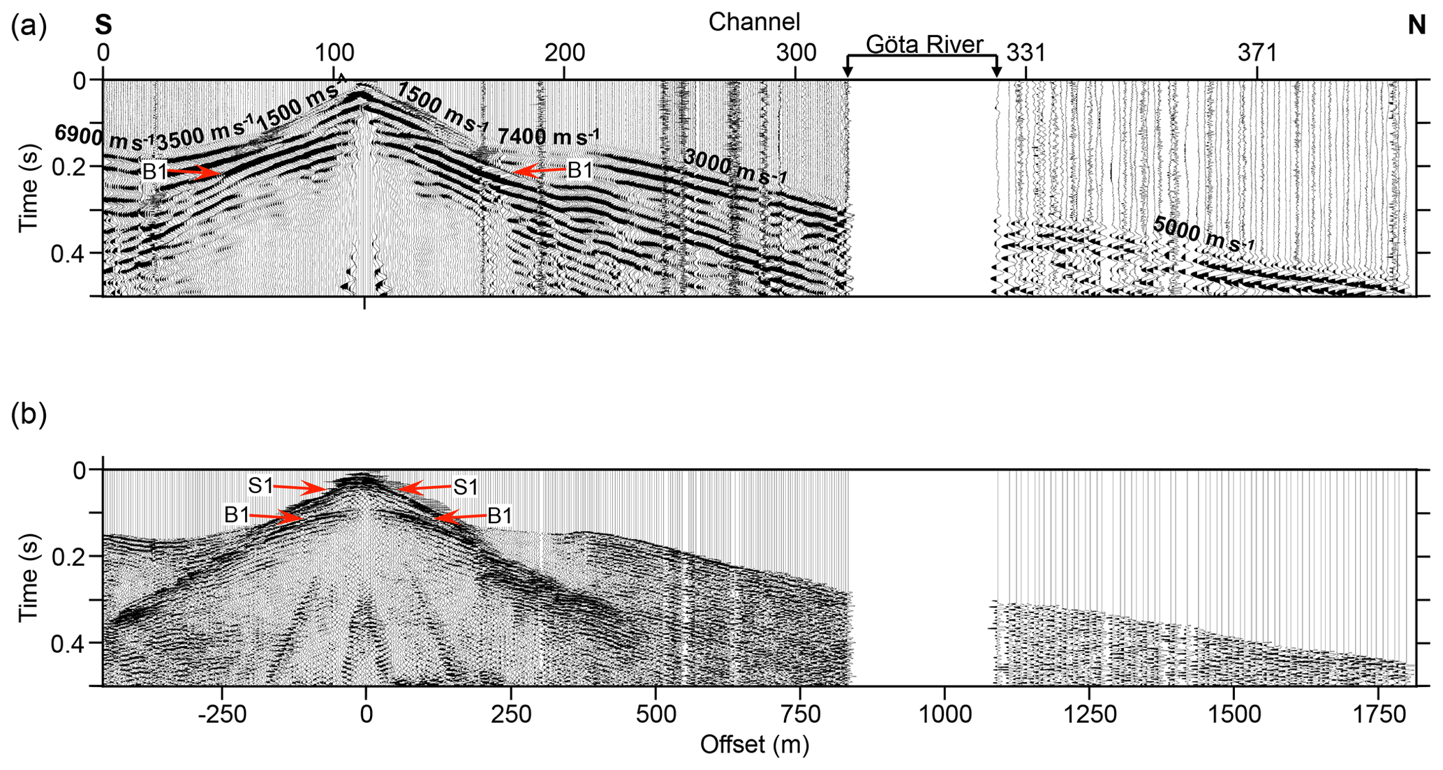
Figure 4 Shot record along line 5–5b (see SH5 in Fig. 2a). (a) Raw shot gather. Apparent velocities for different types of arrivals are shown at the top of each event. (b) Two sets of reflections seem to be revealed, B1 (top of the bedrock) and S1 (top of the coarse-grained materials), after a series of pre-stack processing steps.

The processing of the river reflection seismic data was simpler compared to the land seismic processing (Table S1). In the case of the single-channel data only Wiener deconvolution was applied to remove multiples as much as possible. The six-channel data required the creation of marine geometry according to the receiver and shot positions. A CDP spacing of 1.5 m was used to make the geometry. For the six-channel data more processing steps were necessary, whereby Wiener and post-stack deconvolution helped to improve the final results.

Land and river reflection seismic data were time-to-depth converted using a constant velocity of 1500 m s⁻¹. This value was justified based on the available borehole data for depth calibration. An error on the order of 1–3 m of depth can still be expected, which corresponds to e.g. a 1.3 %–4 % error for a target depth of 75 m.

5 Results and interpretations

5.1 Onshore datasets

Figure 5a–d show, from top to bottom, the seismic results for line 2–2b, the interpreted interfaces, i.e. S1 and B1, and the P-wave refraction tomography and RMT resistivity results obtained in earlier studies (Wang et al., 2016). Figure 5b also includes the natural gamma radiation and magnetic susceptibility data from borehole BH1 (distance to the line 13.4 m; Salas-Romero et al., 2016) and the total sounding data from borehole 7065 (the borehole lies on the line; BGA, 2018). S1 is a subhorizontal interface only identified in the southeastern part of the line; the strong decrease in the gamma log of BH1 and the increase in magnetic susceptibility coincide with this interface. In the northwestern part of the line, next to the river, the S1 reflection is not visible. This interface is the top of the coarse-grained layer previously identified in Salas-Romero et al. (2016). B1, interpreted as the top of the bedrock (BH1 reached the top of the bedrock; see Salas-Romero et al., 2016), is more irregular and has a higher-amplitude reflection than S1. B1 shows a clear undulating morphology, reaching the ground surface at approximately CDP 525 and dipping towards the river in the northwestern side; in borehole 7065 the strong increase in the total sounding curve happens at bedrock depth.

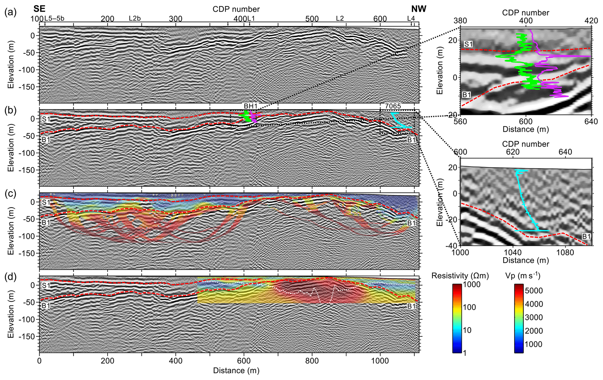
Figure 5 Onshore datasets for line 2–2b. (a) Reflection seismic processing results. On top of the section the corresponding parts of each line and the position of the lines that intersect the merged line are indicated. (b) Interpreted seismic section that includes three borehole datasets: natural gamma radiation (Salas-Romero et al., 2016) in green (ranging from 87 to 182 API) and magnetic susceptibility (Salas-Romero et al., 2016) in purple (ranging from $\mathrm{0.09}\times {\mathrm{10}}^{-\mathrm{6}}$ to $\mathrm{2.2}\times {\mathrm{10}}^{-\mathrm{6}}$ m³ kg⁻¹) from BH1, as well as total sounding (BGA, 2018) from borehole 7065 in blue (ranging from 0 to 15 kN). S1 (top of the coarse-grained materials) and B1 (top of the bedrock) represented by dashed red lines. (c) P-wave refraction tomography model (Wang et al., 2016) superimposed on the interpreted seismic section. (d) RMT resistivity model (Wang et al., 2016) superimposed on the interpreted seismic section. The thin dashed white line indicates the depth above which the results are considered of higher confidence.

Table 3 provides information about the general intervals of P-wave velocities and resistivities for each material identified in the study area (based on the results obtained in Salas-Romero et al., 2016). The P-wave refraction tomography results (Fig. 5c) indicate high velocities (>4000 m s⁻¹) below B1 in the southeastern side but poor ray coverage in the northwestern side. The S1 interface shows for the most part higher velocities (1500–3000 m s⁻¹) compared to the sediments above and below this interface (mostly below 2000 m s⁻¹) in the southeastern part of the line. The resistivity results only cover part of the line (Fig. 5d); above the thin dashed white line, the RMT model is well resolved with high confidence. Wang et al. (2016) estimated the penetration depth (the thin dashed white line position) using a method shown by Spies (1989), and the same criterion is followed for the rest of the lines. Low resistivity values (between 3 and 100 Ωm) are observed above B1 and higher values (>100 Ωm) below, with very high values at the position closer to the surface (up to 1000 Ωm, some outcrops are close to this location; see Fig. 2b). At the S1 position the values are around 80–100 Ωm, which agrees with the material classification (coarse sediment) presented by Solberg et al. (2012). The values immediately above S1, between 10 and 80 Ωm, may indicate silt or leached clay deposits and therefore potential quick clays (Solberg et al., 2012). Quick clay was identified above the coarse-grained layer during visual inspections of the core samples of boreholes BH1 to BH3 (Salas-Romero et al., 2016).

Table 3 General range of P-wave velocities and resistivities for each identified material in the study area.

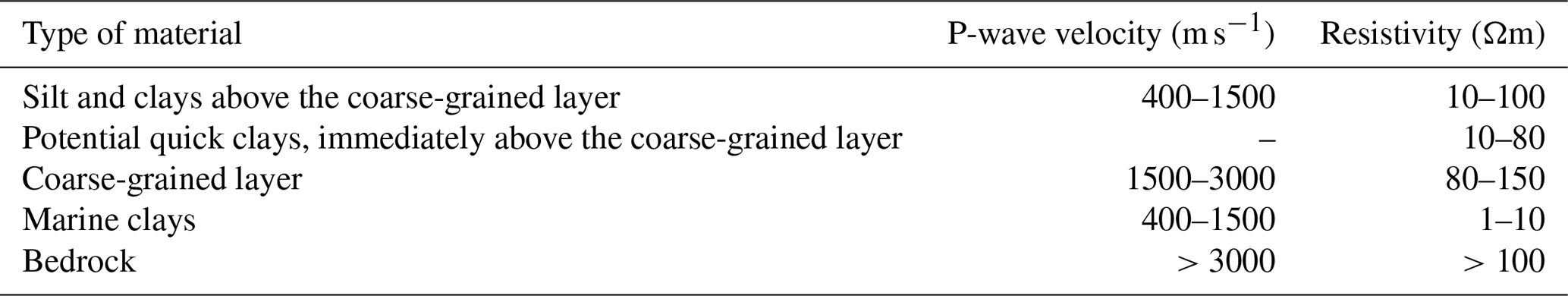
Figure 6a–e show the seismic results for line 5–5b, their interpretation, the earlier P-wave refraction tomography and RMT (Wang et al., 2016), and ATEM resistivity results (Bastani et al., 2017). Figure 6b also includes the natural gamma radiation and magnetic susceptibility data from borehole BH3 (distance to the line 0.23 m; Salas-Romero et al., 2016) and the total sounding data from borehole 7062 (distance to the line 90.3 m; BGA, 2018). Note that the quality of the seismic data is different on each side of the river due to the lower sampling in the northern side (10 m). Nevertheless, the delineation of S1 and B1 is possible along the whole line. The S1 interface shows continuity along the line, except between CDPs 400 and 480. At these positions S1 is not visible, likely due to lower fold in the seismic data (see the fold distribution along line 5–5b in Fig. 6a). Other possibilities cannot be disregarded, e.g. bedrock movement, fractures in the bedrock, and/or deposits disturbed by human activities such as excavation works. A fracture (F) can be inferred in the bedrock at around CDP 440 with some diffraction signatures suggesting the presence of a strong bedrock curvature or edge. The biggest changes in the gamma and magnetic susceptibility logs in BH3 and in the total sounding curve in 7062 coincide with the depth of S1. The undulating B1 reaches close to the surface around CDP 500 and dips to the river after this point; no clear bedrock dipping is observed in the opposite northern shore data. Below the landslide scar, displacement and the oblique translation of some reflections are observed; the sediments appear to have moved towards the river. The top of the bedrock at the river position may be at a depth of around 100 m.

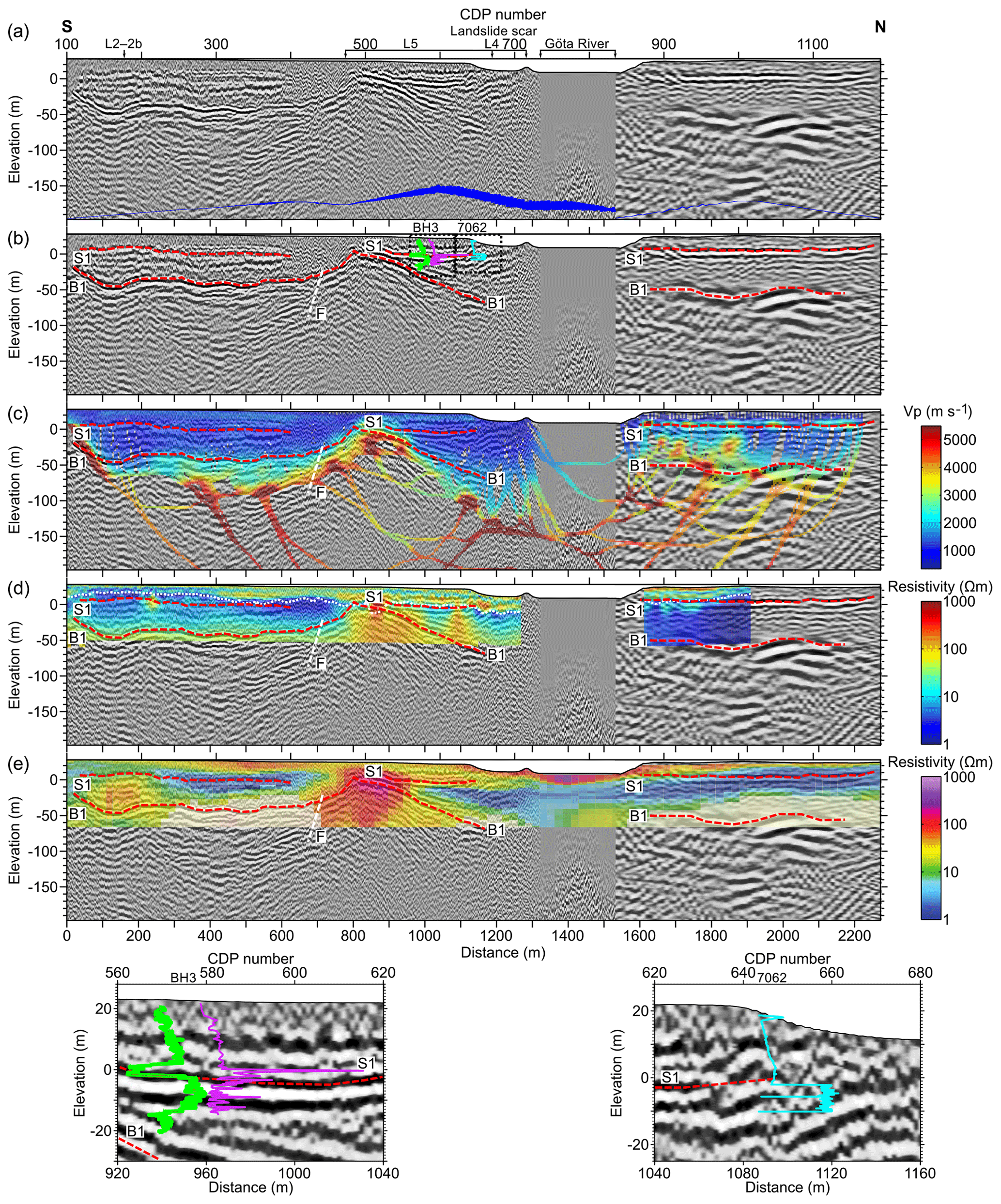
Figure 6 Onshore datasets for line 5–5b. On top of the section the corresponding part of line 5 from 2011, the position of the lines that intersect the merged line, the landslide scar, and the Göta River are indicated. (a) Reflection seismic processing results. The fold distribution along line 5–5b is represented by a blue line at the bottom part of the section (ranging from 0 to 115). In the cabled geophone part (south) the maximum value is 115 and in the wireless part (north) 60. Note the lower fold between CDPs 400 and 480 (minimum value is 47). (b) Interpreted seismic section that includes three borehole datasets: natural gamma radiation (Salas-Romero et al., 2016) in green (ranging from 59 to 200 API) and magnetic susceptibility (Salas-Romero et al., 2016) in purple (ranging from $\mathrm{0.07}\times {\mathrm{10}}^{-\mathrm{6}}$ to $\mathrm{2.7}\times {\mathrm{10}}^{-\mathrm{6}}$ m³ kg⁻¹) from BH3, as well as total sounding (BGA, 2018) from borehole 7062 (ranging from 0 to 12 kN) in blue. S1 (top of the coarse-grained materials) and B1 (top of the bedrock) represented by dashed red lines. F: fractured or disturbed materials, represented by a thick dashed white line. (c) P-wave refraction tomography model (Wang et al., 2016) superimposed on the interpreted seismic section. (d) RMT resistivity results (Wang et al., 2016) superimposed on the interpreted seismic section. The thin dashed white line indicates the depth above which the results are considered of higher confidence. (e) ATEM resistivity results (Bastani et al., 2017) superimposed on the interpreted seismic section.

The P-wave refraction tomography results (Fig. 6c) in the southern side indicate, in general, high velocities (> 3000 m s⁻¹) below B1 and lower velocities in the overlying sediments (between 300 and 1500 m s⁻¹). In the northern side of the line, the tomography results and reflection B1 agree in the northernmost part of the profile, with poor ray coverage below B1. Nevertheless, unexplained velocity artefacts are visible above B1 from the river to CDP 1000. The S1 interface shows higher velocity than the sediments around it in the northern part of the line, which is similar to what is observed in Fig. 5c. In contrast, the southern part of the line does not show any velocity difference at the S1 interface. The RMT resistivity values (Fig. 6d) are mostly high (>100 Ωm) below B1, although the northern side does not have data below the top of the bedrock. Above B1, the RMT resistivity values are low (between 1 and 10 Ωm) except along S1, where the values reach >100 Ωm. The values immediately above S1 may indicate leached clay deposits (potential quick clays; Solberg et al., 2012). In the southern part of the profile, between 100 and 250 m of distance, the ATEM resistivity values (Fig. 6e) show a high-resistivity anomaly above the interface B1, which is not observed in the RMT resistivity results. In the northern part of line 5–5b the penetration depth of the ATEM model does not reach the position of B1. In comparison, the ATEM resistivity results seem to delineate the interface S1 between CDPs 500 and 700 and between 880 and 1000. Malehmir et al. (2016) interpret a possible fault (low resistivity values sandwiched between high resistivity values identified as bedrock) on the southern shore of the river between CDPs 730 and 750 at approximately 30 m below sea level.

Figures S1a–c and S2a–d in the Supplement show similar seismic results for lines 6 and 7, their interpretation, and the earlier obtained P-wave refraction tomography and RMT resistivity results (Wang et al., 2016). Figure S2b also includes the total sounding data from borehole 7075 (distance to the line 1.6 m; BGA, 2018). B1 is delineated along both lines (Figs. S1b and S2b), showing undulating morphology, approaching the ground surface in the eastern side and dipping towards the river in the western side. In contrast, the S1 reflection is only delineated between CDPs 100 and 210 in line 7 (Fig. S2b). Borehole 7075, located in the western side of the line, shows strong increases in the curves at the S1 interface. In Fig. S1b, between CDPs 100 and 200 from −50 to −100 m of elevation, a different reflection pattern (dipping to the east of the line) is present, which may be related to 3-D effects caused by the rough bedrock topography. Fractured or disturbed materials (F) are identified in the western side of line 6 (Fig. S1b). The F materials located seem to coincide with a probable fracture zone present in Fig. 2a, which runs parallel to the river profile. The P-wave refraction tomography results (Figs. S1c and S2c) are similar for both lines. The velocities are high in the eastern side (>3000 m s⁻¹) below B1 and low in the overlying sediments (approximately between 450 and 2000 m s⁻¹). In the western side of the lines the ray coverage is poorer at the depth of B1. The resistivity values in line 7 are high (>100 Ωm) below B1 in the eastern side (Fig. S2d); the western side does not have resistivity results below B1 and only partial results above it. The resistivity values are around 10 to 100 Ωm at shallower depths, except at the S1 position and below it where the values are lower, between 1 and 10 Ωm. In terms of resistivity, these values do not indicate coarse sediments but unleached marine clay deposits (Solberg et al., 2012).

5.2 Offshore datasets

Figure S3a–b show the seismic processing results for the single-channel data (©SGU) and their interpretation, respectively. The seismic results still show many multiples along the line, e.g. between 2000 and 3500 m of distance or between 9000 and 11 000 m of distance. Six filled channels labelled with the letter C (Fig. S3b) can be distinguished along the line; the larger ones up to 2000 m wide are found in the first 11 000 m of distance, and the smaller ones are around 1000 m wide. Only a peak in the bedrock interface (B1) is interpreted between 5500 and 6000 m of distance, separating two adjacent channels. The interpretation of the areas separating adjacent channels in the rest of the cases, at distances around 2800, 8000, 11 500, 13 000, and 15 000 m, is complicated because no more structures are clearly visible. The reasons may include the bedrock being very close to the surface and/or the presence of fracture zones as shown in the interpretation of the six-channel data.

The results of the six-channel data collection (©SGU) and their interpretation are presented in Fig. 7a and b, respectively. Figure 7b also includes the total sounding data from boreholes 11 014, 11 034, and 11 094 (BGA, 2018). The difference in height between the valleys and peaks reaches up to 15 m (Fig. 7a). Although the resolution of the six-channel data compared to the single-channel data is lower, geological features can be distinguished at greater depth (>100 m). In the interpreted section (Fig. 7b) the same channels (C) identified in the single-channel data (Fig. S3b) can also be delineated, as can the bedrock highs between 5500 and 6000 m of distance (there is a difference of about 10 m in height between the two datasets at this point, probably due to the distance between the lines). Strong variations in the borehole data coincide with the filled channel positions. The bedrock undulates and presents several fracture zones between CDPs 800 and 1000, 1350 and 1400, 2350 and 2500, and 2950 and 3000. These fracture zones coincide with fracture zones identified using the geological information provided by SGU (Fig. 2a). In Fig. 7b we can also observe that the reflection amplitude decreases between CDPs 3000 and 5402, the deeper areas being more affected. The bedrock interface (B1) may be closer to the surface at these positions, and thus the low-amplitude region would represent the transparent crystalline bedrock.

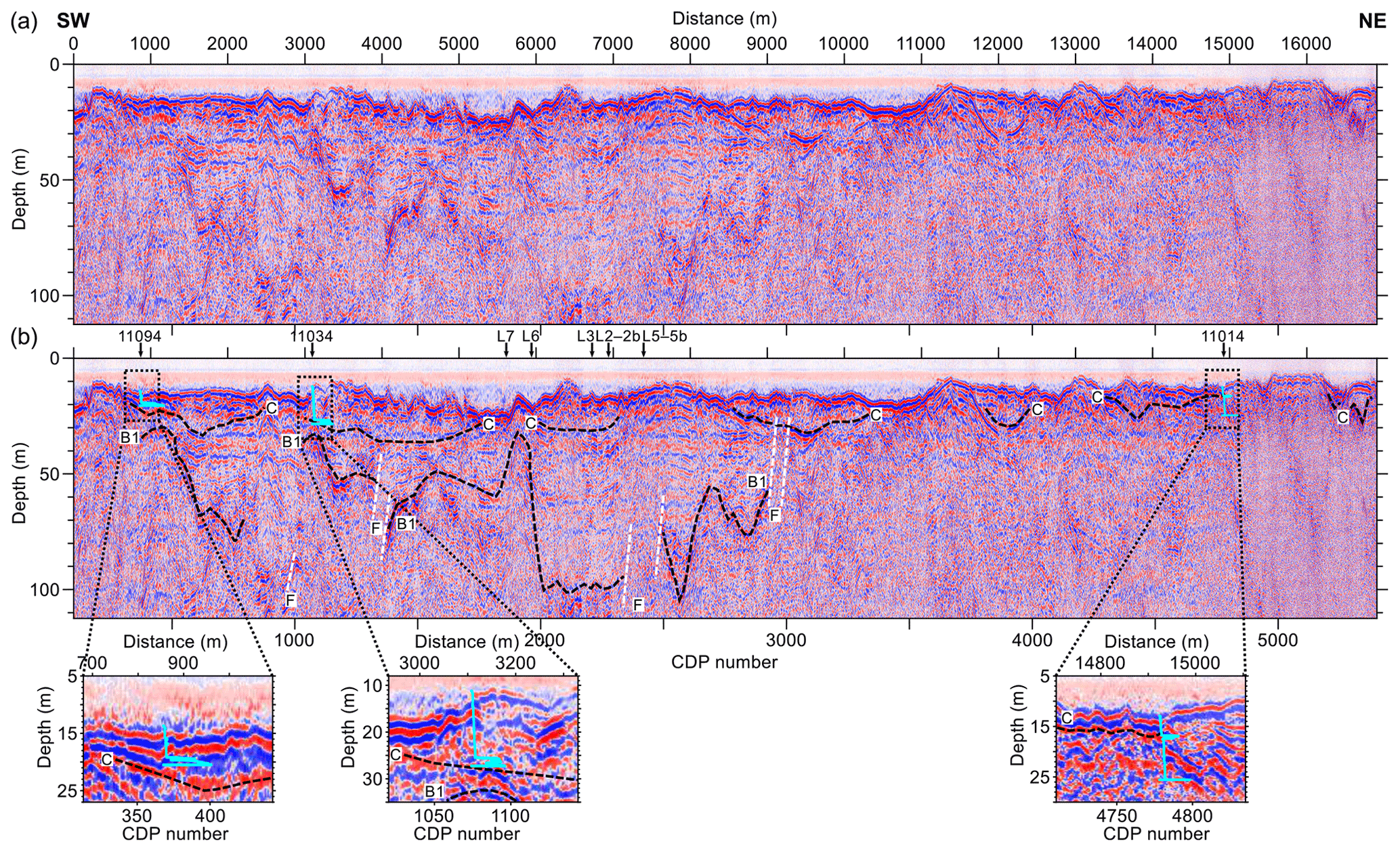
Figure 7 Offshore datasets for the six-channel river line (©SGU). (a) Seismic processed section. (b) Interpreted seismic section including total sounding data (BGA, 2018) from boreholes 11 014 (ranging from 0 to 7.2 kN, distance to the line 45 m), 11 034 (ranging from 0 to 9.2 kN, distance to the line 10 m), and 11 094 (ranging from 0 to 11.2 kN, distance to the line 25.7 m), all in blue. C: filled channels, B1: top of the bedrock represented by dashed black lines, and F: fractured or disturbed materials (no reflection continuity) represented by a dashed white line. The positions of the land seismic lines that intersect this line are indicated on top of the section. Scale 1H : 30V.

Figure 8 shows a detailed section of the river seismic data (©SGU) between CDPs 1800 and 3300. The portion of side-scan sonar data (©SGU) corresponding to the profile A–A^′ (Fig. 8b–c) is presented in Fig. 8a. Figure 8b–c show the interpreted sections of single- and six-channel data. Line 5–5b crosses a fracture zone. In Fig. 8a hummocks and disturbed riverbed are observed at the centre of the river bottom; these may be interpreted as landslide debris. The shade colour and the texture may indicate denser and coarser deposits, respectively, compared to their surrounding materials. In Figs. 2a and 6a, at the position of line 5–5b, a landslide scar is found in the southern side of the river. In the opposite riverbank two more landslide scars are found as is one gully flowing from the south and a tributary flowing from the southeast (Fig. 2a–b). Based on Fig. 8a, it is unclear whether the deposits at the river bottom originate from the landslides or are fluvial sediments.

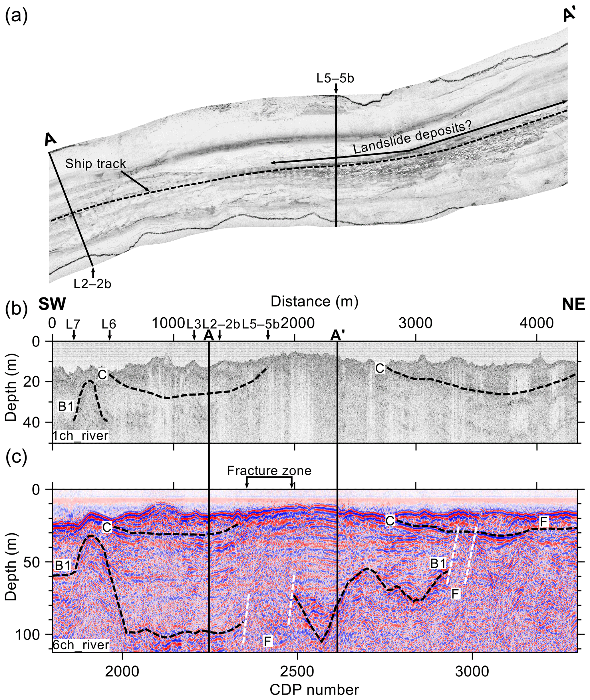
Figure 8 A section of the river seismic lines and side-scan sonar data (©SGU). (a) Side-scan sonar data corresponding to the profile A–A^′ shown on top of the section in (b). (b) Interpreted single-channel seismic section. Scale 1H : 12V. (c) Interpreted six-channel seismic section. Scale 1H : 12V. The positions of the land seismic lines that intersect the lines are indicated on top of (b). C: filled channels, B1: top of the bedrock, F: fractured or disturbed materials (no reflection continuity).

6 Discussion

6.1 3-D modelling of the subsurface materials

One of the main objectives of this study was to obtain the extension of the coarse-grained layer and its spatial relationship with the bedrock surface. Malehmir et al. (2013a, b) have shown that the coarse-grained layer extended locally in a restricted area, but this work shows the extension of this layer to the north and south of the initial study area. The top of the coarse-grained layer and the top of the bedrock were picked on the processed land and river seismic lines, and elevation surfaces were interpolated using the seismic, borehole (BGA, 2018), and lidar data (©Lantmäteriet). Total sounding data identify the top and bottom of the coarse-grained layer at many points at the site. The lidar data were used to fix the elevation of the rock outcrops. The elevation surfaces for the top of the coarse-grained layer and the top of the bedrock (Fig. 9a and b) were calculated using a natural neighbour interpolation after a Delaunay triangulation of the scattered sample points was generated. The results are better constrained in the area surrounding the rock outcrop, as more seismic lines are available there. The top of the bedrock is visible in all the lines, except line 4 (Malehmir et al., 2013b), and therefore the model of the bedrock surface in the study area is generally well constrained. The top of the coarse-grained layer is not identified in line 6, but the model gives a good overview of the layer extension, which spreads over both sides of the river. The maximum elevations for both the top of the bedrock and top of the coarse-grained layer surfaces occupy the centre of the survey site, and the undulated bedrock dips down towards the river. The latter implies that more water may flow in the coarse-grained layer closer to the river. Löfroth et al. (2011) and Salas-Romero et al. (2016) show that the coarse-grained layer is thicker within the depressions, which is related to the deeper top of the bedrock and sediment focusing when deposition took place. The thickness of the coarse-grained layer and the higher water flow could increase the thickness of potential quick clays in those depressions. We interpret the combination of the coarse-grained layer, bedrock morphology, and the presence of fractured bedrock to contribute to the formation of quick clay and to be likely preconditioning factors for a landslide (see e.g. L'Heureux et al., 2017).

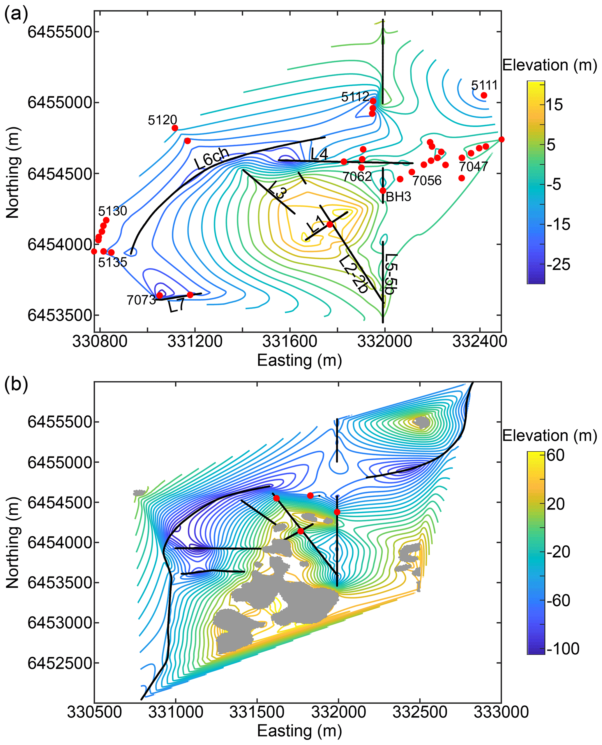
Figure 9 Elevation contours for the interpolated surfaces of (a) the top of the coarse-grained layer (contour spacing 3 m) and (b) the top of the bedrock (contour spacing 6 m). The data used for the interpolation are picked points along the seismic lines for each interface (black lines), the borehole data (red dots), and lidar data for the rock outcrops (grey areas). Note that only selected boreholes are labelled, but all indicated boreholes were used for the interpolation (most of the borehole data can be found in BGA, 2018).

Figures S4 and S5 show different perspectives of this modelling together with the 3-D visualization of the seismic profiles. In Fig. S4c, two elongated depressions next to the river, which cross lines 2–2b, 5–5b, 6, and 7, can be identified. These depressions are interpreted as possible faults and coincide with the position of mapped fracture zones (Fig. 2a). The possible faults indicate areas more susceptible to slide, together with the slope inclination and/or increased water flow. Figure S5b shows the strong bedrock undulation between lines 6 and 7, whose reflection seismic results (Figs. S1 and S2) indicate 3-D effects in the western part of the profiles due to rough topography. The reflection corresponding to a filled channel correlates with the interpolated top of the coarse-grained layer surface (Fig. S5b).

6.2 Hydrological modelling of the coarse-grained layer

After obtaining the elevation surface for the top of the coarse-grained layer, we modelled the elevation surface for the bottom of the layer using the RMT resistivity (Lindgren, 2014; Shan et al., 2014; Wang et al., 2016) and available borehole data (BGA, 2018; Salas-Romero et al., 2016). Thickness values of the coarse-grained layer were picked along the RMT resistivity profiles at its estimated position. The thickness of the layer was then interpolated together with thickness values obtained from the borehole data. The interpolated thickness surface was subtracted from the elevation surface of the top of the coarse-grained layer previously modelled in order to obtain the elevation surface of the bottom of the coarse-grained layer.

The typical soil sequence and groundwater system in the Göta River valley is, from top to bottom, (i) an altered clay layer with increased transmissivity potentially reaching down to 5 m and acting as an upper aquifer, then (ii) more intact clay beds acting as an aquitard underlain by (iii) a lower aquifer consisting of a coarser layer of sand or till, and/or weathered or fractured bedrock (Persson et al., 2011). This framework was applied to the site to interpret pore pressure measurements available at different depths for an array of sites (BGA, 2018) and water levels at the boreholes BH1 to BH3 (Table S2). The water pressure looks close to hydrostatic near the ground surface before decreasing to a minimum above the estimated depth of the coarse-grained layer, which is found to have a higher pressure than the overlaying clays, sometimes even displaying artesian conditions (Tables S2 and S3). This would indicate that little to no groundwater recharge is occurring through the clay down to the coarse-grained layer. The pressure values in the coarse-grained layer exhibit a decreasing trend when travelling from the higher-elevation outcrops in the centre of the study area down to the river (Table S2, and Fig. 10a). The central part of the model is characterized by the disappearance of the coarse-grained layer, a thin sandy–silty till cover, and several elevated rock outcrops (Fig. 2a), which we hypothesize to be a groundwater recharge area for the coarse-grained layer by infiltration along the bedrock–sediment interface. The coarse-grained layer seems to be hydraulically connected to the river, at least intermittently.

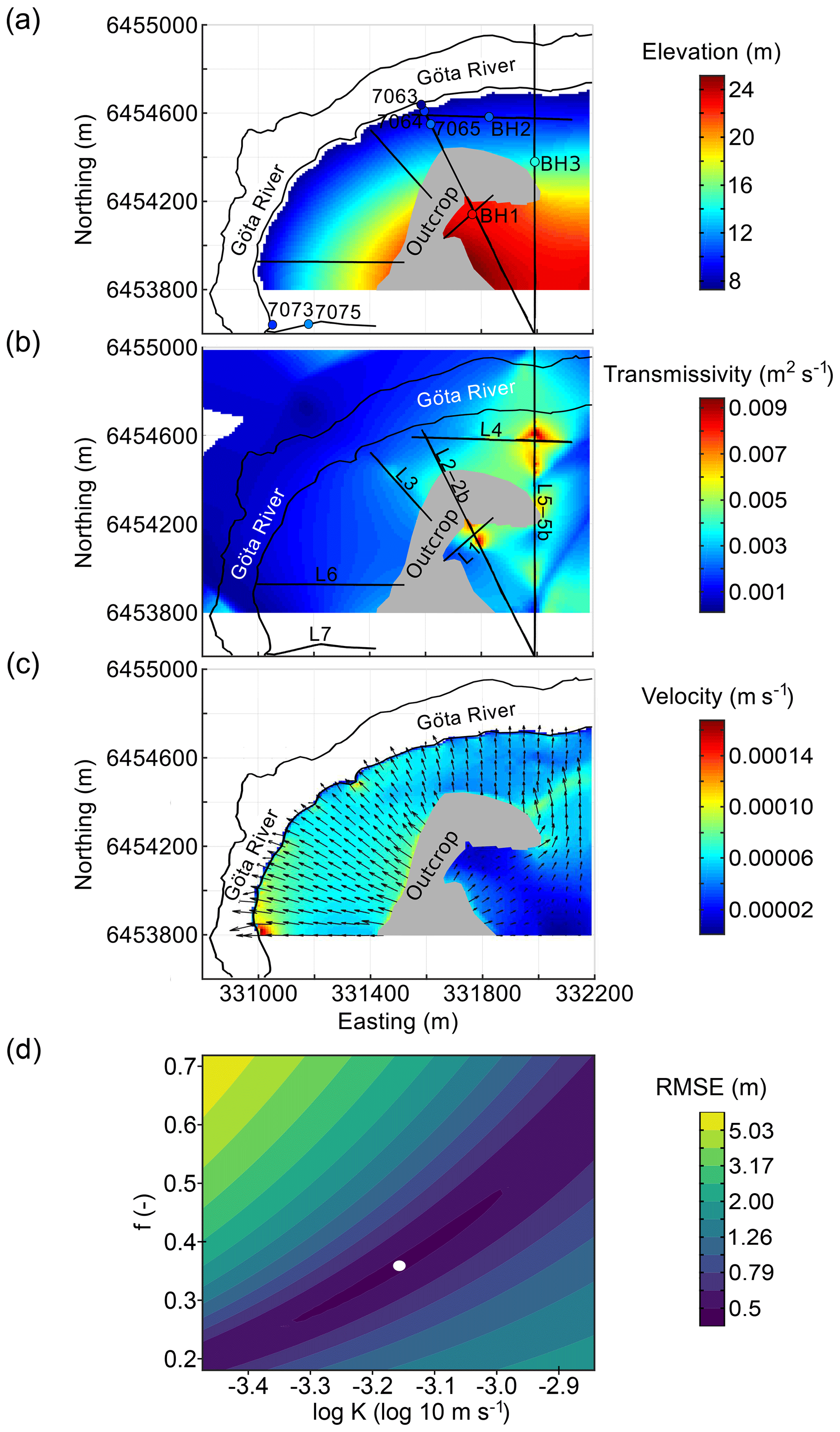
Figure 10 Hydrological modelling of a selected region in the study area. (a) Water table elevation. (b) Transmissivity distribution. (c) Mean groundwater velocity distribution and vector field of the Darcy flow. The positions of the Göta River, outcrop area, land seismic lines (Malehmir et al., 2013a, b; Salas-Romero et al., 2016), and boreholes (BGA, 2018; Salas-Romero et al., 2016) used in the modelling are indicated in the figure. (d) RMSE distribution. The white circle indicates where RMSE is minimum and equal to 0.5 (log K is about −3.15 and the groundwater recharge over the recharge zone is about 36 % of the normal net precipitation for this area).

To test these insights, the elevation and thickness values for the coarse-grained layer were used to build a single-layer two-dimensional confined aquifer model for the coarse-grained layer (Fig. 10a) governed by the steady-state groundwater flow Eq. (1) (Bear, 1972):

$$\begin{array}{}\text{(1)}& \mathrm{\nabla }\cdot \left(T\mathrm{\nabla }h\right)=\mathrm{0},\end{array}$$

where the hydraulic head (h) is the unknown variable. A horizontal model resolution of 10 m was chosen and the problem was solved using a finite-volume method (Guyer et al., 2009). The transmissivity (T) was defined as the product of the local interpolated coarse-grained layer thickness with a uniform hydraulic conductivity (K); the latter needed to be calibrated (Fig. 10b). The transmissivity values are higher (from 0.0035 to 0.0095 m² s⁻¹) around the land seismic lines due to a thicker coarse-grained layer at these positions. As hydraulic boundary conditions, the cells directly underlying the river were assumed to have a fixed head corresponding to the average river level as shown in Fig. 2b. The area of the considered recharge zone (A) is approximately 0.2 km², and the groundwater recharge rate was used as a calibration parameter. The recharge area was represented as a fixed flux boundary condition to the adjacent coarse-grained layer cells. Consistent with the vertical pore pressure profiles, the groundwater recharge rate over the rest of the model domain (outside the recharge zone) was deemed unlikely to exceed 5 % of the normal annual mean net precipitation (P_net) in the catchment estimated at around 460 mm yr⁻¹ (Swedish Meteorological and Hydrological Institute – SMHI, 2018) and was effectively set to zero.

Eight groundwater level and pore pressure values from the existing boreholes in the study area or measured near the depth of the coarse-grained layer (see Fig. 10a and Table S2) were used as targets to fit the log 10 value hydraulic conductivity (log K) of the coarse-grained layer and the recharge rate over the central outcrops (expressed as a fraction f of the annual mean net precipitation). The calibration was obtained by minimizing the root mean square error (RMSE) on the eight modelled pressure values following a conjugate gradient method. The model approaches the targets with an RMSE of less than 0.5 m for an effective log K value of $-\mathrm{3.15}\pm \mathrm{0.15}$ (or K=0.0007 m s⁻¹), which is plausible for a coarse sandy layer, and a recharge rate over the central part of the model of about 165 mm yr⁻¹, which is about 36 % (±10 %) of the normal net precipitation for this catchment (SMHI, 2018; Fig. 10d).

According to this model, the groundwater recharge through the top fine-grained sediment layers is of second order to explain the hydraulic behaviour of the coarse-grained layer. Artesian conditions can be found on low grounds near the river, sometimes only at peak flow conditions. A calculation of the water residence time (τ) in the coarse-grained layer can be done according to Eq. (2):

$$\begin{array}{}\text{(2)}& \mathit{\tau }={\displaystyle \frac{V\times \mathit{\varphi }}{A\times P_{\mathrm{net}}\times \mathrm{0.36}}},\end{array}$$

which is approximately 48 years, assuming a porosity (ϕ) of 0.3 (or 30 %) and a calculated volume V of the coarse-grained layer of 5 hm³. This relatively short residence time would point to lower-salinity groundwater occurrences in the coarse-grained layer compared to the overlying clays and ion transfer from the clays to the underlying groundwater flow system by diffusion (Torrance, 1979) and/or by seasonal inflow–outflow cycles of groundwater flow between the coarse-grained layer and the overlying clays, which has been identified as a precursor to the formation of quick clays (Rankka et al., 2004).

Figure 10c shows the values of the mean groundwater velocity (Darcy flow vector amplitude divided by ϕ) and vector field of the Darcy flow, whose directions go from the outcrop area to the river. At positions where T (or the thickness of the coarse-grained layer) is lower (less than 0.0035 m² s⁻¹), the mean groundwater velocity is higher (from 0.00006 to 0.00010 m s⁻¹) and vice versa; where T is large (from 0.0035 to 0.0095 m² s⁻¹) the velocity is very low (less than 0.00007 m s⁻¹). Assuming that the leaching of marine salts increases with groundwater velocity, areas where the groundwater velocity is higher could be at increased risk of quick-clay formation.

6.3 Morphology of the Göta River valley

The total-field magnetic data were corrected for differences in diurnal variations and instrumental drift using the base station data (a background International Geomagnetic Reference Field – IGRF – value of 50 600 nT was subtracted from the results to convert to residual magnetic anomaly data). However, several inconsistencies were still present in the corrected data, such as different values at overlapping positions, level jumps between measurement days (see the sketch with the measurement and base station positions in the lower right corner in Fig. 11a), and elongated features parallel to the measuring paths. In order to level the data, a constant value was added or removed in the measurements for the last 3 d, and the polarity was changed for the data of the first day. For removing the elongated features, the data were divided in two groups, the first 3 d and the last 2 d of measurements, gridded, and filtered similar to the micro-levelling procedure (Minty, 1991). A low-pass filter was applied in the N–S direction, a high-pass filter was applied in the E–W direction, and then the result was subtracted from the original gridded data. The final result (Fig. 11a) is smoother and more homogeneous than the initial data but still has a few elongated features, which are residual errors (acquisition footprint) and not natural features as they coincide with the sampling directions.

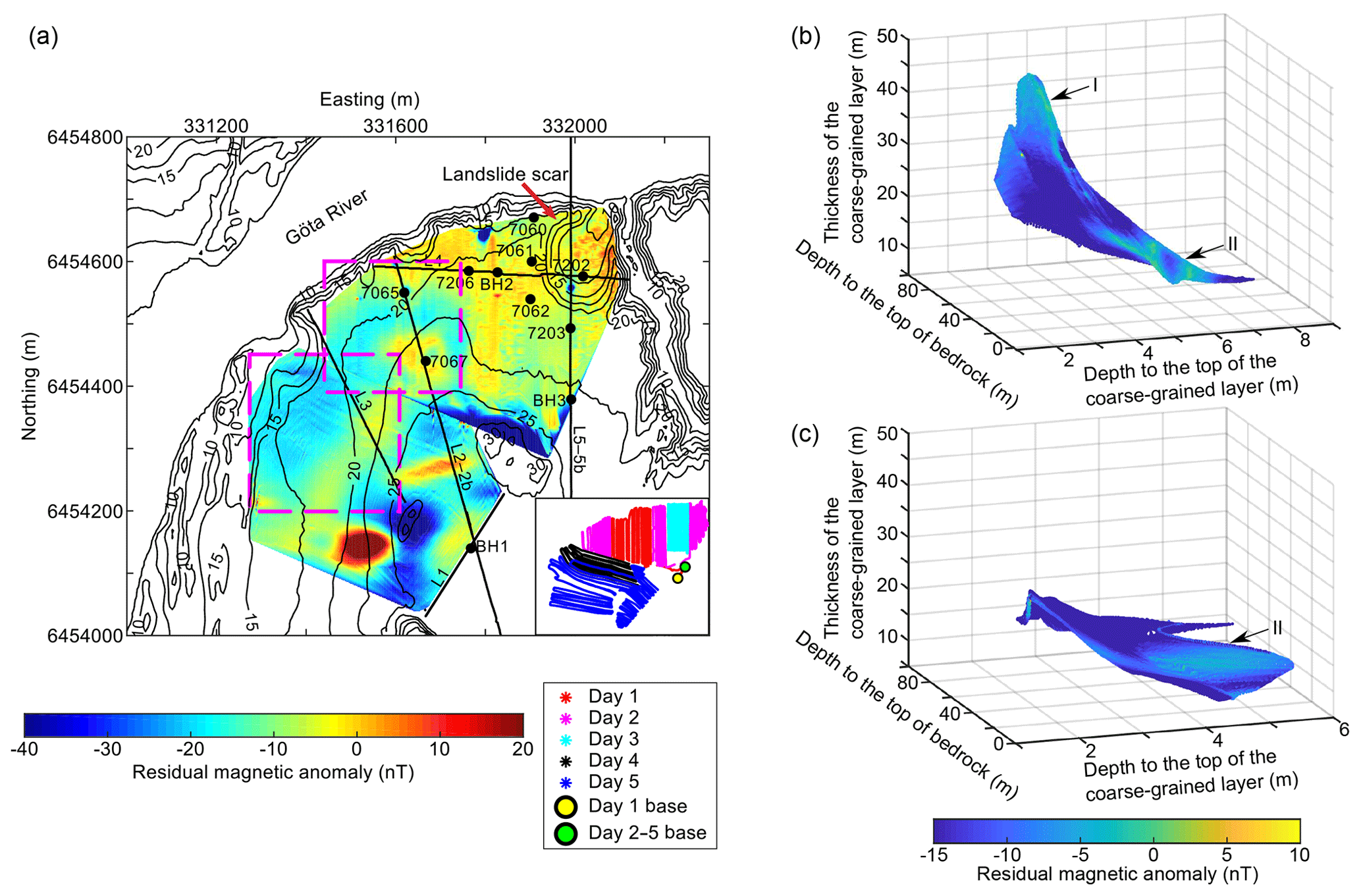
Figure 11 Residual magnetic anomaly data in (a) map view over the lidar elevation contour plot (©Lantmäteriet), (b) cross-plot with depth to the top of the bedrock and the top of the coarse-grained layer, and the thickness of the latter for the northern area (top magenta box in a). (c) Cross-plot with the same variables for the southern area (bottom magenta box in a). The position of the land seismic lines (Malehmir et al., 2013a, b; Salas-Romero et al., 2016) and boreholes (BGA, 2018; Löfroth et al., 2011; Salas-Romero et al., 2016) used for analysing the magnetic data as well as a sketch of the measurement and base station positions for each day are shown in (a).

Figure 11a shows that the residual magnetic anomaly values are higher on the northern part than on the southern (ranging from −20 to 20 nT); at the bottom and in the eastern flank of the landslide scar that crosses line 5–5b the values reach 20 nT. Almost all along line 4 and between lines 2–2b and 5–5b higher residual magnetic anomaly values are found. Salas-Romero et al. (2016) showed that the coarse-grained layer has higher magnetic susceptibility compared to the sediments above and below these materials. We also took samples at the bottom of the landslide scar up to 1.5–2 m of depth that were identified as silty–sandy. The high residual magnetic anomaly values at the landslide scar may indicate that the coarse-grained layer, which drains the water infiltrated from the nearby outcrops and/or fractures, may have acted as a sliding surface together with quick clays. L'Heureux et al. (2012) identified a “weak layer” composed of softer and more sensitive clays and sands (compared to the surrounding materials) that acted as a slide-prone layer in the initiation of the 1996 Finneidfjord landslide. This layer also contained biogenic gas, which may have affected its geotechnical properties. Biogenic gas was found in boreholes BH2 (Salas-Romero et al., 2016) and 7075 (BGA, 2018), which adds another similarity with the case described in L'Heureux et al. (2012). According to the farmer working these lands the landslide scar was formed approximately 50 years ago, and the landslide could have been triggered due to changes in the river water level, an increase in pore pressure, and/or toe erosion. Looking at the borehole information available in the area (BGA, 2018; Löfroth et al., 2011; Salas-Romero et al., 2016), the top of the coarse-grained layer lies between 10 and 30 m of depth, being deeper at boreholes 7206 and BH2. At the latter borehole, the thickness of the coarse-grained layer reaches almost 10 m (in BH1 and BH3 the thickness of this layer is about 1 and 3 m, respectively). The shallowest tops of the coarse-grained layer are registered at borehole 7202, at the landslide scar, and at BH1. Comparing this information with the residual magnetic anomaly data, we infer that the coarse-grained layer, its distance to the surface, and its thickness may be related to the high values of the magnetic data in the northern part and around BH1 where line 1 lies. The bedrock at these positions is quite deep to cause such high values (e.g. in BH2 the top of the bedrock is around 78 m). The southwestern part does not reflect the same behaviour, which may be related to the thinness of the coarse-grained layer and/or its depth. On the southern part of the residual magnetic anomaly map an elongated anomaly that follows the SW–NE direction is observed. The values are higher in the centre (ranging approximately between −15 and 5 nT), with the maximum values around borehole 7067 (BGA, 2018) at the intersection with line 2–2b, and lower around the anomaly (ranging from −25 to −15 nT). At borehole 7067, bedrock is close to the surface, with high residual magnetic anomaly values coinciding with the bedrock topography. We interpret the elongated anomaly to be related to the scarp formed between the bedrock and the lower elevated sediments to the west (Fig. 2). The southeastern part of the residual magnetic anomaly map, where there are several outcrops and the surface elevation is higher, includes negative and positive magnetic anomalies. A few houses and farms may have influenced the residual magnetic anomaly data in this area.

In order to test how the high values of the residual magnetic anomaly relate to the thickness of and depth to the top of the coarse-grained layer, as well as to the depth to the top of the bedrock, the different variables have been compared for two selected areas, a northern and a southern one (see magenta boxes in Fig. 11a). The northern area includes the northern tip of the SW–NE elongated anomaly mentioned earlier. A 3-D cross-plot of the above-mentioned variables exhibits two clusters of high values of the residual magnetic anomaly (Fig. 11b). The high values in one of the clusters seem to be related to the large thickness of the coarse-grained layer and/or the shallow depth to the top of this layer (see label I in Fig. 11b). The second cluster of high values is located at a deeper depth to the top of coarse-grained layer and the lower thickness of this layer, but instead the top of the bedrock is shallower (see label II in Fig. 11b). Similar clustering related to the depth of the top of the bedrock is observed in the southern area (Fig. 11c). Other areas more to the north have been tested and the results show a mix of trends (including residual errors), which makes interpretation difficult. This suggests that the residual magnetic anomaly data are complex but correlate positively with the presence of the coarse-grained layer and/or bedrock.

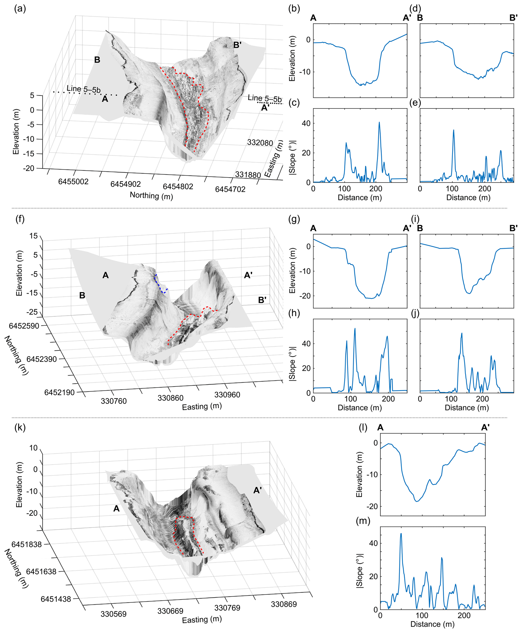
Figure 12 Side-scan sonar data (©SGU) overlying the bathymetric data (©SGI) on selected segments of the Göta River. See the position of the figures in Fig. 2c. (a, f, k) Cross sections of the river. Scale 1H : 8V, 1H : 3V, and 1H : 4V, respectively. The areas delineated with a dashed red line show accumulated material at the bottom of the river and in the margins, and the dashed blue line delineates a probable subaquatic landslide scar. (b, d, g, i, l) Elevation along profiles A–A^′ and B–B^′. (c, e, h, j, m) Slope (absolute values) along profiles A–A^′ and B–B^′.

Figure 12 presents three examples of combining the side-scan sonar (©SGU) with the bathymetric data (©SGI) on the river (see the positions in Fig. 2c). The first example, Fig. 12a–e, is a section that is crossed by line 5–5b. Deposits of unclear origin can be observed at the bottom of the section (Fig. 12a); their granular texture and darker colour indicate that they may be harder and denser than the surrounding materials. These deposits may proceed from the landslide scars in both sides of the river (Fig. 2) and/or from the discharge of sediments transported by the gullies or tributary intersecting the Göta River at this position. Slopes in profile A–A^′ can be classified as “high terrace-steep slope” (Millet, 2011), with values ranging between 30 and 45^∘. Profile B–B^′ (Fig. 12d–e) shows the same type of slope on the northern riverbank and a gentler slope (the slope is a mix between “high terrace-steep slope” and “straight uneven profile”; Millet, 2011) on the opposite side. The B^′ extreme coincides with the position of a stream (Fig. 2). The toe of the slope probably contains material due to the collapse of the subaquatic slope or sediments deposited by the stream. The second example, Fig. 12f–j, is a section located south of the study area. Profile A–A^′ shows a possible subaquatic landslide scar in the western side. Figure 12g–h shows a “double terrace” (slopes between 40 and 55^∘) on the western side and a “high terrace-steep slope” (inclination around 47^∘) on the opposite side. The deepest terrace in the western side has a ledge that is around 5 m high, which coincides with the position of the identified subaquatic landslide scar. Profile B–B^′ (Fig. 12i–j) shows accumulated material against the riverbank in the eastern side. The slope on the western side can be classified as a “high terrace-steep slope” (slope ∼50^∘), and the slope profile on the opposite side resembles a combination of the classes “high terrace-steep slope” and “straight uneven profile” (maximum slope is around 30^∘). The toe of the slope seems to consist of landslide deposits. The third example, Fig. 12k–m, is a section even more to the south than the one in Fig. 12f–j. Accumulated material is visible at the bottom of the river in the eastern side in profile A–A^′ (Fig. 12l). The inclination of the slope is very irregular, generally below 20^∘ but with some parts having higher inclination. The slope looks like a “straight uneven profile”, although there are parts with small terraces. The toe of the slope appears to have formed from landslide deposits. The opposite side resembles a “high terrace-steep slope” (slope is 45^∘).

Erosion and landslide processes have formed the landscape of the Göta River valley (SGI, 2012a). Land and river seismic data, together with side-scan sonar and bathymetric data, give a good overview of the (sub)surface in this valley. Along the river filled channels are identified, which were probably formed when the riverbed morphology changed over time. The bedrock at the river channel shows several fracture zones. The slopes of the riverbanks are generally steep, and many subaquatic landslide scars and deposits can be found along the river. The origin of these deposits may also be related to the remains of erosion protections placed between 1960 and 1970 along the Göta River. The likelihood of retrogressive landslides inland can increase due to the undercutting of riverbanks during high discharge or wave erosion generated by shipping movement, which reduces lateral support and causes more instability (SGI, 2012a). At the surface, the inclination of the slopes is influenced by land use and precipitation-induced processes (SGI, 2012a).

According to SGI, our study area has, in general, medium landslide risk. Close to the river the risk is higher due to the presence of highly sensitive clays or quick clays. SGI has evaluated the risk of landslides along the Göta River under different climate change scenarios (SGI, 2012a). These scenarios estimate increases in temperature by 4–5^∘ and 20 %–30 % more precipitation by 2100. High and low drainage levels from Lake Vänern will be more frequent, sea level will rise by up to 0.7 m at Göteborg, and maximum groundwater levels and pore pressure in slopes will not change significantly. These conditions could increase the occurrence of landslides and modify the valley morphology in the future (SGI, 2012a). Erosion has a great impact to the south of Lilla Edet and under these climate change scenarios will be more intense along the river's course (SGI, 2012a). This means that although the study area is located to the north of Lilla Edet, where erosion has less impact, any small change in the erosion rate in the future could cause serious effects as this area is already considered to be at medium–high landslide risk.

7 Conclusions

Through an extensive reflection seismic investigation, which includes four new land seismic profiles as well as the incorporation of existing profiles, river lines, and their combination with other geophysical, geotechnical, and borehole data, this study allows for the large-scale delineation of a coarse-grained layer, underlying bedrock, and fracture zones in an area prone to quick-clay landslides in southwest Sweden. This is the first time in Sweden that land and river reflection seismic data are combined to study the subsurface associated with this type of landslide.

Some of the geological and geohydrological prerequisites for the formation of quick clay in nature specified by Rankka et al. (2004) are shown in the results of this study. The correlation of reflection seismic, resistivity, and P-wave refraction tomography results offers information about the presence of underlying coarse-grained layers, peaks in the bedrock surface, and the approximated thickness and type of clay deposits. 3-D subsurface morphology modelling of the coarse-grained layer and bedrock illustrates the possible infiltration points in the area as nearby elevated rock outcrops or fractures. Hydrological modelling of the coarse-grained layer suggests that the dominant leaching processes are diffusion and/or seasonal inflow–outflow cycles of the groundwater flow between the coarse-grained layer and the overlying clays. The formation of quick clays is more significant under artesian groundwater conditions that can be found in the low-elevation grounds near the river at the survey site. Ground residual magnetic anomaly data are positively correlated with the thickness of and distance to the coarse-grained materials and bedrock topography. The northern part of the study area contains a shallower and thicker coarse-grained layer. At the bottleneck landslide scar present in the centre of the survey, the high residual magnetic anomaly values are most likely due to the presence of the coarse-grained layer (containing magnetic minerals), which suggests that it may have acted as a sliding surface together with quick clays, similar to the “weak layer” identified by L'Heureux et al. (2012) in Norway. The side-scan sonar and bathymetric data reveal a number of distinct morphological features in the Göta River valley that reflect erosional processes, landslide scars, and mass-movement deposits.

This work illustrates the significance of studying subsurface geology, including features within bedrock that are often overlooked when investigating landslides, especially ones that involve quick clays.