The impact of rheological uncertainty on dynamic topography predictions

Much effort is being made to extract the dynamic components of the Earth's topography driven by density heterogeneities in the mantle. Seismically mapped density anomalies have been used as an input into mantle convection models to predict the present-day mantle flow and stresses applied on the Earth's surface, resulting in dynamic topography. However, mantle convection models give dynamic topography amplitudes generally larger by a factor of ∼2, depending on the flow wavelength, compared to dynamic topography amplitudes obtained by removing the isostatically compensated topography from the Earth's topography. In this paper, we use 3-D numerical experiments to evaluate the extent to which the dynamic topography depends on mantle rheology. We calculate the amplitude of instantaneous dynamic topography induced by the motion of a small spherical density anomaly (∼100 km radius) embedded into the mantle. Our experiments show that, at relatively short wavelengths (<1000 km), the amplitude of dynamic topography, in the case of non-Newtonian mantle rheology, is reduced by a factor of ∼2 compared to isoviscous rheology. This is explained by the formation of a low-viscosity channel beneath the lithosphere and a decrease in thickness of the mechanical lithosphere due to induced local reduction in viscosity. The latter is often neglected in global mantle convection models. Although our results are strictly valid for flow wavelengths less than 1000 km, we note that in non-Newtonian rheology all wavelengths are coupled, and the dynamic topography at long wavelengths will be influenced.

1 Introduction

The Earth's mantle is continuously stirred by hot upwellings from the core–mantle boundary and by subduction of colder plates from the surface into the deep mantle (Pekeris, 1935; Isacks et al., 1968; Molnar and Tapponnier, 1975; Stern, 2002). This introduces temperature and density anomalies that stimulate mantle flow and forces dynamic uplift or subsidence at the plates' surfaces (Gurnis et al., 2000; Braun, 2010; Moucha and Forte, 2011; Flament et al., 2013). Dynamic topography can affect the entire planet's surface with varying magnitudes. Because it is typically a low-amplitude and long-wavelength transient signal, it is often dwarfed by isostatic topography associated with variations in the thickness and density of sediments, crust and mantle lithosphere.

For the present day, the observational constraints on dynamic topography come from residual topography measurements (Hoggard et al., 2016). Residual topography is calculated by removing the isostatically compensated topography from the Earth's topography (Crough, 1983; Cazenave et al., 1989; Davies and Pribac, 1993; Steinberger, 2007, 2016). The comprehensive work from Hoggard et al. (2016) revealed that residual topography varies between ±500 m at very-long wavelengths (i.e. ∼ 10 000 km) and can increase up to ±1000 m at shorter wavelengths (i.e. ∼1000 km). However, these residuals depend on our knowledge of the thermal and mechanical structure of the lithosphere and therefore may not be an accurate estimation of the deeper mantle contribution to the Earth's topography. Another approach to constrain present-day Earth's dynamic topography involves numerical modelling of present-day mantle flow using seismically mapped density anomalies as an input (Steinberger, 2007; Moucha et al., 2008; Conrad and Husson, 2009). However, this method requires a detailed knowledge of the viscosity structure in the Earth's interior (Parsons and Daly, 1983; Hager, 1984; Hager et al., 1985; Hager and Clayton, 1989), and translating seismic velocities to physical properties (e.g. temperature) of the mantle introduces further uncertainties (Cammarano et al., 2003). The problem is that dynamic topography predictions derived from mantle convection models are generally larger by a factor of 2 (more significant at the very-large scales) than estimates from residual topography (Hoggard et al., 2016; Cowie and Kusznir, 2018; Davies et al., 2019; Steinberger et al., 2019). We hypothesise that this could be related to an oversimplification of the mantle rheology. In this paper, we explore how, at wavelengths <1000 km, the magnitude of dynamic topography changes when we use a rheological model in which the viscosity depends on strain rate, temperature, pressure and fluid content. We first summarise the well-established analytical solution for calculating dynamic topography induced by a spherical density anomaly embedded into an isoviscous fluid (Morgan, 1965a; Molnar et al., 2015). Then, assuming isoviscous rheology, we illustrate that the amplitude of dynamic topography depends on the viscosity structure of the Earth's interior as shown by Morgan (1965a) and Molnar et al. (2015). Finally, we use 3-D coupled thermo–mechanical numerical experiments of the Stokes flow to assess the dependence of dynamic topography on nonlinear rheology using viscosity which depends on temperature, pressure, strain rate and fluid content. We show that plausible nonlinear rheologies can induce local variations in viscosity and result in dynamic topography of lower amplitude compared to those derived from models using isoviscous rheology.

2 Dynamic topography driven by a rising sphere: analytical and numerical solutions

2.1 Analytical solution for one layer isoviscous fluid

We assume here a simple 2-D model representing a very-viscous spherical density anomaly embedded into a semi-infinite isoviscous fluid bounded by an upper free surface. Earliest analytical investigations revealed that, albeit counter-intuitive, the magnitude of the induced surface deflection due to the rising sphere is independent of the viscosity of the fluid. The dynamic topography is a function of the vertical total stress (σ_zz) applied to the surface which is proportional to the size and depth of the density anomaly according to Eq. (1) (Morgan, 1965a, b):

$$\begin{array}{}\text{(1)}& {\mathit{\sigma }}_{zz}\left(x,\mathrm{0}\right)=\left[\mathrm{2}g\mathit{\delta }\mathit{\rho }{r}^{\mathrm{3}}\right]{\displaystyle \frac{D^{\mathrm{3}}}{{\left(D^{\mathrm{2}}+x^{\mathrm{2}}\right)}^{\mathrm{5}/\mathrm{2}}}},\end{array}$$

where g is the gravitational acceleration, δρ is density difference between the anomaly and the ambient material, r is radius of the sphere, and D is distance from the surface to the centre of the anomaly (modified from Morgan, 1965a, see Fig. 1a). The dynamic topography e is given by the following:

$$\begin{array}{}\text{(2)}& e\left(x\right)={\displaystyle \frac{{\mathit{\sigma }}_{zz\left(x,\mathrm{0}\right)}}{g\mathrm{\Delta }\mathit{\rho }}}\mathrm{at}z=\mathrm{0},\end{array}$$

where Δρ is the density difference between the mantle and air (or water assuming a sea-load when e<0) (Morgan, 1965a; Houseman and Hegarty, 1987). In Fig. 1a, we plot the dynamic topography induced by a sphere of 1 % density anomaly, whose centre is at 372 km depth (D=372 km) below the free surface. We calculate the vertical total stress and convert it to dynamic topography by using Eq. (2) for different values of the radius of the sphere. The amplitude of dynamic topography shows an accelerating increase by cubic dependence on the radius of the spherical density anomaly (Fig. 1a, solid black line). For the same problem, Molnar et al. (2015) provided a solution by considering a higher-order term, resulting in a slight difference from the solution of Morgan (1965a) (see Appendix A3 in Molnar et al., 2015), which allows the consideration of density anomalies of finite viscosity (η_sphere) (Eq. 3):

$$\begin{array}{}\text{(3)}& \begin{array}{rl}{\mathit{\sigma }}_{zz}\left(C,\mathrm{0}\right)& ={\displaystyle \frac{-\mathit{\delta }\mathit{\rho }{r}^{\mathrm{3}}D}{\mathrm{3}f}}[{\displaystyle \frac{\mathrm{3}-\mathrm{2}f}{C^{\mathrm{3}}}}+{\displaystyle \frac{\mathrm{18}\left(f-\mathrm{1}\right)r^{\mathrm{2}}}{C^{\mathrm{5}}}}\\ & +{\displaystyle \frac{\mathrm{6}f{D}^{\mathrm{2}}}{C^{\mathrm{5}}}}-{\displaystyle \frac{\mathrm{30}(f-\mathrm{1})r^{\mathrm{2}}{D}^{\mathrm{2}}}{C^{\mathrm{7}}}}],\end{array}\end{array}$$

where $C=\sqrt{D^{\mathrm{2}}+x^{\mathrm{2}}}$, and $f=({\mathit{\eta }}_{\mathrm{1}}+\frac{\mathrm{3}{\mathit{\eta }}_{\mathrm{sphere}}}{\mathrm{2}})/({\mathit{\eta }}_{\mathrm{1}}+{\mathit{\eta }}_{\mathrm{sphere}})$. One can find that f=1.5 if the sphere is very viscous (η_sphere≫η₁), and f<1.5 for any other case. In Fig. 1a, we present two more plots of dynamic topography where f=1.5 for hard sphere and f=1.25 for η_sphere=η₁ by using Eqs. (2) and (3). Figure 1a shows that a rising deformable sphere creates higher dynamic topography compared to a very-viscous sphere. These show that the viscosity contrast between the spherical anomaly and the surrounding material can affect the dynamic topography. In the section that follows, we explore how dynamic topography varies when there is layering in viscosity such as the presence of a strong lithosphere above the convective mantle.

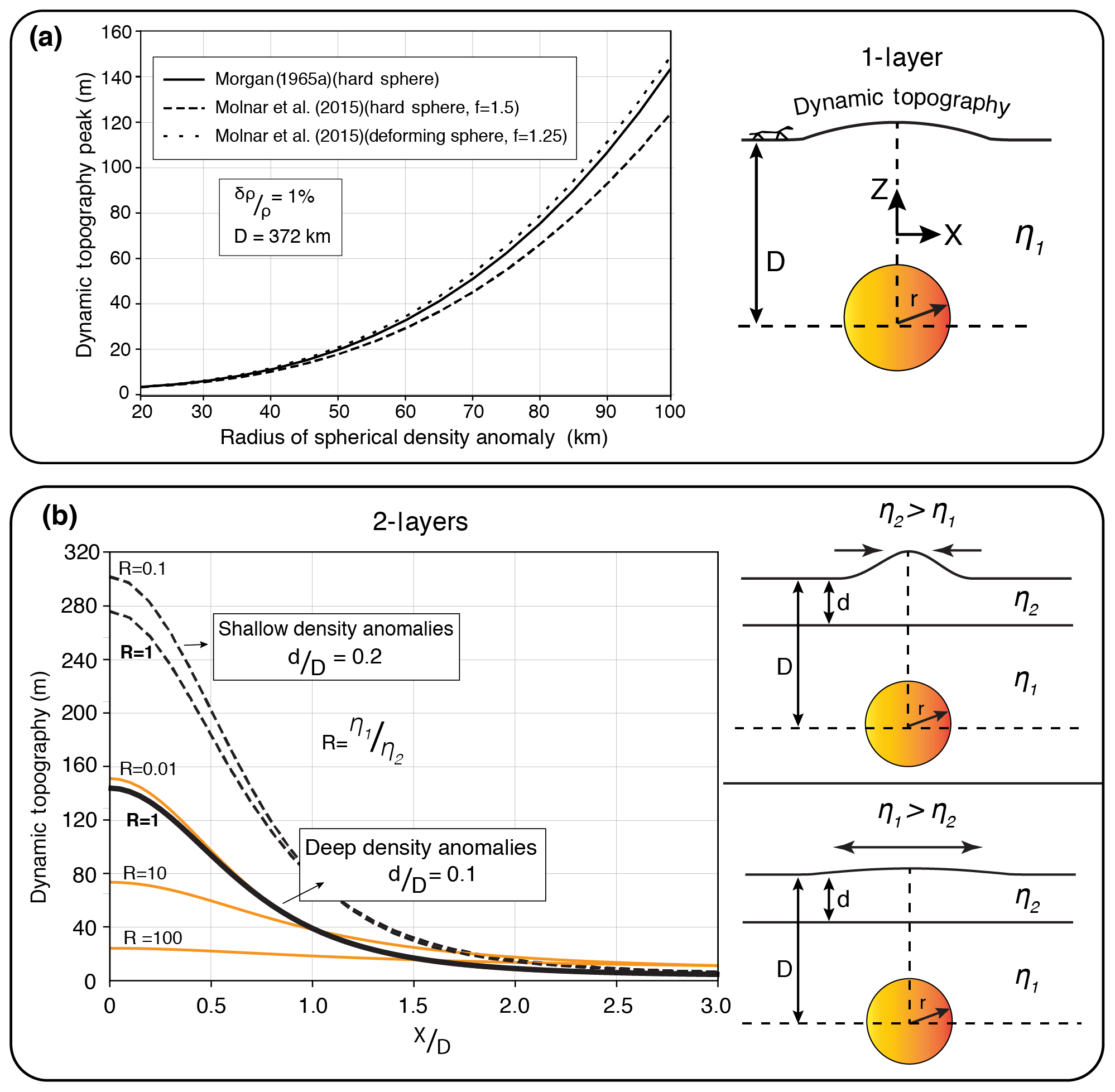
Figure 1 Dynamic topography driven by a spherical density anomaly of radius r at depth D embedded in a fluid whose viscosity structure is varied. (a) Variation in dynamic topography by radius of a spherical 1 % density anomaly centred at 372 km depth in a single isoviscous fluid whose viscosity is η₁. The normal total stresses are calculated by Eq. (1) taken from Morgan (1965a) (hard sphere) and Eq. (3) taken from Molnar et al. (2015) (hard and deforming spheres), and converted to dynamic topography by using Eq. (2). (b) The case where the fluid is no longer a single layer but is composed of two layers with viscosities η₁ and η₂ for the lower and upper layers, respectively. We plot the dynamic topography for the same density anomaly in (a) using Eq. (4), taken from Morgan (1965a), but with varying relative viscosities ($R={\mathit{\eta }}_{\mathrm{1}}/{\mathit{\eta }}_{\mathrm{2}}$). The ratio of upper-layer thickness to depth to the centre of the anomaly (d∕D) also affects the dynamic topography, and higher values correspond to shallow density anomalies or thicker lithosphere for constant depth (D).

2.2 The impact of layered viscosity structure on dynamic topography

A more generalised solution has been put forward to accommodate the presence of a stronger upper layer representing a lithosphere with viscosity η₂ above a weaker layer with viscosity η₁, and with η₁<η₂ representing the convective mantle (Fig. 1b). In this case, Morgan (1965a) showed (Eq. 4) that the total normal stress induced by the density anomaly is dependent on the mass anomaly per unit length (M_u, for point sources integrated along a continuous line), the depth of the centre of the sphere (D) and marginally on the ratio of the viscosity of the convective mantle to the viscosity of the lithosphere ($R={\mathit{\eta }}_{\mathrm{1}}/{\mathit{\eta }}_{\mathrm{2}}$). The 2-layer problem is treated in Fourier domain with the resulting total normal stress as below:

$$\begin{array}{}\text{(4)}& {\mathit{\sigma }}_{zz}\left(x,\mathrm{0}\right)=\underset{\mathrm{0}}{\overset{\mathrm{\infty }}{\int }}{\mathit{\sigma }}_n\cos nx\mathrm{d}n,\end{array}$$

where

$$\begin{array}{rl}{\mathit{\sigma }}_n& ={\displaystyle \frac{M_{u}g{e}^{-n(D-d)}}{\mathrm{2}\mathit{\pi }(R{S}_h+C_h)}}\mathit{\{}\mathrm{1}+n\left(D-d\right)\\ & +nd\left[{\displaystyle \frac{\mathrm{1}-nD+n(D-d)(R{C}_h+S_h)/(R{S}_h+C_h)}{\mathrm{1}+nd(\mathrm{1}-R^{\mathrm{2}})/(R{S}_h+C_h)(R{S}_h+S_h)}}\right]\mathit{\}},\end{array}$$

C_h=cosh (nd), S_h=sinh (nd) and d is the upper-layer thickness (modified from Morgan, 1965a). Following Morgan (1965a), Fig. 1b illustrates the relative importance of R as well as the ratio of the thickness of the upper layer to the depth of the anomaly (d∕D). As long as the lithosphere is more viscous than the asthenosphere, the vertical total stress at the surface has a minor dependence on the viscosity of the lithosphere (see solid lines with R=1 and R=0.01 in Fig. 1b). Figure 1b also shows that the magnitude of dynamic topography increases as the density anomaly is brought closer to the surface (compare R=1, the solid black line and the dashed black line). Moreover, its sensitivity on the relative viscosity of the lithosphere also increases. Although an unrealistic proposition for the Earth, when the lithosphere is less viscous than the asthenosphere, the normal stress is much reduced and is strongly dependent on the viscosity of the lithosphere (Fig. 1b). These demonstrate that layering in viscosity can have a strong impact on the amplitude of dynamic topography (Sembroni et al., 2017). In the next section, we use the analytical solutions above to benchmark a numerical model, which we will then extend to nonlinear viscosity.

2.3 Numerical solutions

For comparison with analytical solutions (Morgan, 1965a; Molnar et al., 2015), we consider 3-D numerical models involving 1, 2 and 3 isoviscous layers. These benchmark experiments will be used as references for non-isoviscous models discussed in Sect. 3. We use the open-source code Underworld which solves the Stokes equation at insignificant Reynolds number (Moresi et al., 2003, 2007). The 3-D computational grid represents a domain 3840 km × 3840 km × 576 km with a resolution of 6 km along the vertical z axis and 10 km along the x and y axes (Fig. 2). In all experiments, we include a 42 km thick continental crust above the upper mantle. The density structure is sensitive to the geotherm via a coefficient of thermal expansion and compressibility (see Table 1 for all parameters). The geotherm is defined using a radiogenic heat production in the crust, a constant temperature of 20 ^∘C at the surface and a constant temperature of 1350 ^∘C at 150 km. We disregard the adiabatic heating, and the asthenosphere is kept at 1350 ^∘C. We embed a positive spherical temperature anomaly of +324 ^∘C at a depth of 372 km below the surface, which delivers a 1 % volumetric density difference. The radius of the sphere is 96 km. In all experiments, we impose free slip velocity boundary conditions at all walls, such as V_x and V_y are set to be free, but V_z=0 cm yr⁻¹ at the top wall. Taking advantage of the symmetry of the experimental setup, we extract viscosity and velocity fields along a 2-D cross section passing through the centre of the thermal anomaly, from which we derive the streamlines and vertical velocity profiles along the vertical axis at the centre of the models. We calculate the instantaneous dynamic topography from the normal stress computed at the surface.

Table 1 Thermal and rheological parameters.

n/a – not applicable. We use the rheological parameters from ^a quartzite (Ranalli, 1995), ^b dry or wet olivine (Hirth and Kohlstedt, 2003).

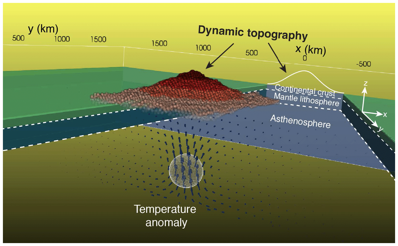
Figure 2 Three-dimensional numerical model of a spherical temperature anomaly having 96 km radius and a density of 1 % less dense than the ambient mantle embedded in a depth of 372 km. The model space is 3840 km long in x and y axes, and 576 km deep along the z axis. The dynamic topography is depicted as an exaggerated surface on the top of the model and is also reflected on the x−z plane.

2.3.1 Dynamic topography due to a rising sphere in an isoviscous fluid

In the first experiment (Fig. 3a Experiment 1), we assign the same depth-independent viscosity of 10²¹ Pa s to the crust, mantle and the density anomaly. The streamlines for Experiment 1 (Fig. 3a) show formation of two convective cells at the sides of the sphere covering the entire crust and mantle. The vertical velocity profile indicates that the thermal anomaly rises with a peak velocity of ∼2.4 cm yr⁻¹, which is faster than the 2.0 cm yr⁻¹ predicted by the analytical solution (Fig. 4a). Experiment 1 predicts dynamic topography of 114 m (Fig. 4b) which is lower than 132 m predicted by the analytical solution of Molnar et al. (2015). We have verified that increasing the depth of our model from 576 to 864 km increases the dynamic topography from 114 to 122 m. Therefore, we attribute the misfit in amplitude of dynamic topography to the finite space in our numerical experiments. Our numerical experiment using isoviscous material delivers a result globally consistent with the analytical solutions of Morgan (1965a) and Molnar et al. (2015).

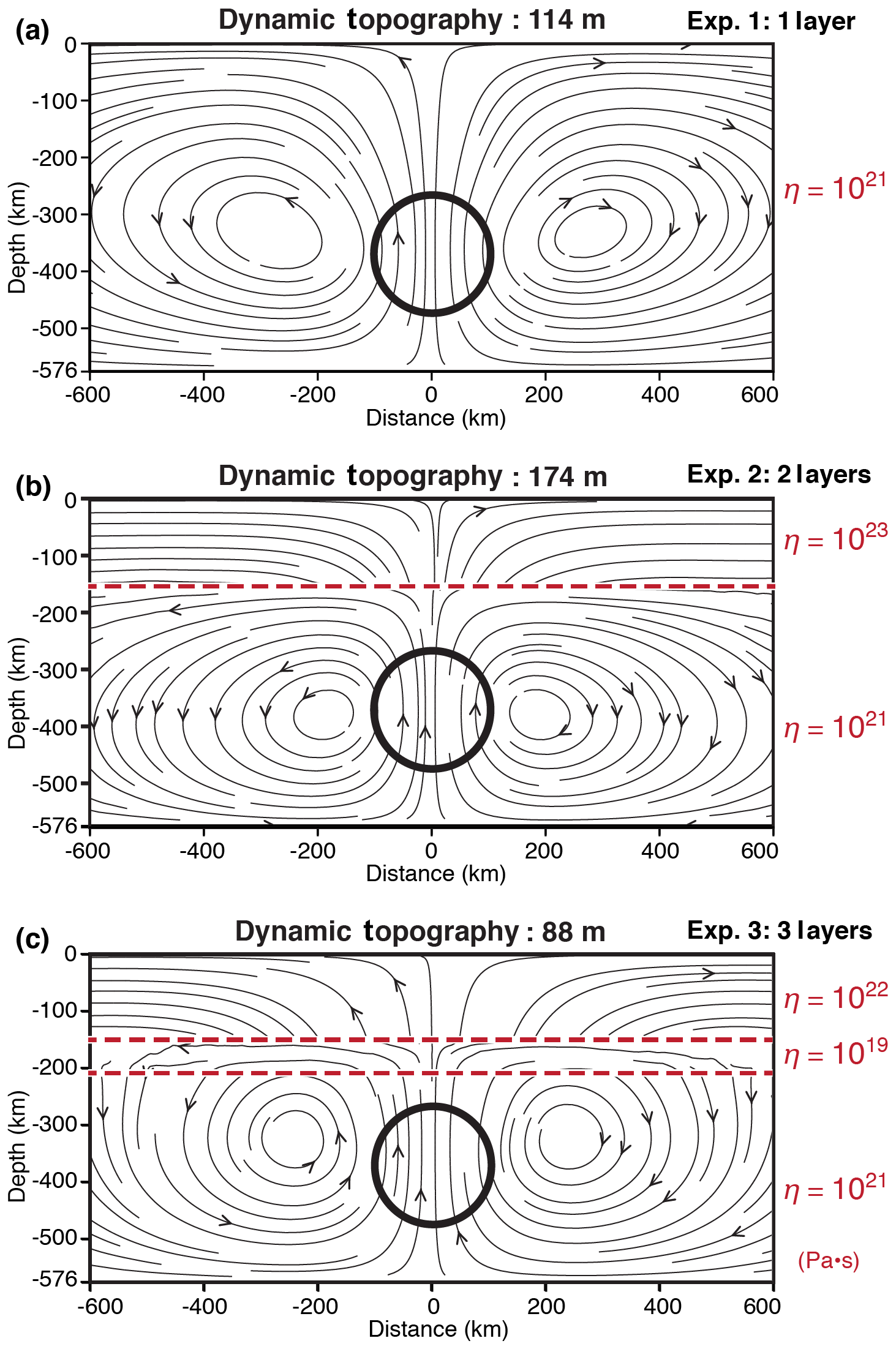
Figure 3 Predicted peak amplitudes of dynamic topography for layered Earth models with isoviscous rheology. Centred at 372 km depth, the embedded spherical density anomaly (black circle) is 96 km in radius. It has a temperature anomaly of +324 ^∘C, giving 1 % effective density difference with the background. The resulting streamlines are shown in a 2-D cross section (x−z plane) along the centre of each numerical model (y=0 km).

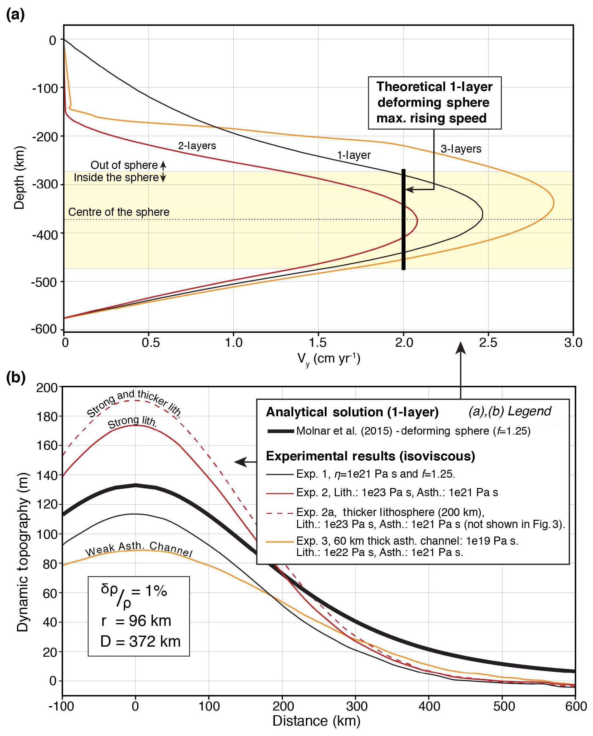
Figure 4 (a) Vertical velocity profiles (V_y) along the centre, and (b) analytical solution and numerical modelling results showing dynamic topography induced by a sphere of temperature anomaly in the mantle (r=96 km, $\mathit{\delta }\mathit{\rho }/\mathit{\rho }=\mathrm{1}$ %). The misfit between the numerical model for R=1 and the analytical solution is due to finite space in the numerical model compared to semi-infinite space assumed in the analytical solution (Morgan, 1965a).

2.3.2 Dynamic topography on a strong lithosphere above an isoviscous asthenosphere

In Experiment 2, we assign to the lithosphere a constant viscosity 100 times larger (10²³ Pa s) than that of the asthenosphere (10²¹ Pa s, Fig. 3b) between z=150 km and base of the model. The convective cells become narrower by the induced viscosity contrast (Fig. 3b). The streamlines are deflected across the lithosphere–asthenosphere boundary due to the large viscosity contrast (Fig. 3b), and there is a sharp variation in vertical velocity at the base of the lithosphere (Fig. 4a, solid red line). The maximum vertical velocity ∼2.1 cm yr⁻¹ is attained near the centre of the anomaly. When compared to Experiment 1, the dynamic topography (Fig. 4b, solid red line) shows a significant increase from ∼114 to ∼174 m. This increase is consistent with analytical estimations showing an increase in dynamic topography when viscosity increases toward the surface (Fig. 1b, R<1). In Experiment 2a (not shown here), we tested a different ratio of thickness of the lithosphere to the depth of the anomaly (see d∕D in Eq. 4) by increasing the lithospheric thickness from 150 to 200 km, while keeping all parameters identical to those of Experiment 2. As predicted by Eq. (4), Exp. 2 predicted dynamic topography of ∼191 m, being the largest among all experiments (Fig. 4b, dashed red line). Overall, and perhaps counter-intuitively, the presence of a thick viscous lithosphere enhances the dynamic topography. Interestingly, in analogue experiments where density anomaly is allowed to rise and interact with the lithosphere, the amplitude of the dynamic topography is inversely correlated with the thickness of the lithosphere (e.g. Griffiths et al., 1989; Sembroni et al., 2017).

2.3.3 The impact of low-viscosity channel on the dynamic topography

In Experiment 3 (Fig. 3c), we introduce a third 60 km thick low-viscosity layer (i.e. 10¹⁹ Pa s) beneath the base of the lithosphere. The existence of a low-viscosity layer has been discussed in several studies (e.g. Craig and McKenzie, 1986; Phipps Morgan et al., 1995; Stixrude and Lithgow-Bertelloni, 2005; Becker, 2017). In this experiment, in order to prevent large viscosity contrast that can impede the numerical convergence, the viscosities of the lithosphere and that of the asthenosphere are set to 10²² and 10²¹ Pa s, respectively. When compared to Experiment 1, streamlines indicate a further decrease in size of the convective cells and more importantly, a strong horizontal divergence of the streamlines within the low-viscosity layer (Fig. 3c). The vertical velocities are also enhanced in the asthenosphere reaching up to ∼ 2.8 cm yr⁻¹ slightly above the centre of the anomaly (Fig. 4a, solid orange line). When compared to Experiment 1, we observe a strong reduction in dynamic topography (Fig. 4b, solid orange line) from 114 to 88 m. This is due to the damping effect of the low-viscosity channel that acts as a decoupling layer, which reduces the deviatoric stress through its ability to flow.

Until now, the viscosities were assumed to be constant. However, results from experimental deformation on mantle rocks strongly suggest that the viscosity is highly nonlinear (Hirth and Kohlstedt, 2003). In what follows, we explore the influence of more realistic viscosities on dynamic topography.

3 The impact of nonlinear viscosity on dynamic topography

3.1 Viscosity structure of the Earth's interior

The Earth's mantle is not isoviscous. Geological records of relative sea level changes related to postglacial rebound, geophysical observations of density anomalies inferred from seismic velocity variations in the mantle and satellite measurements of the longest wavelength components of the Earth's geoid have been used to infer the radial viscosity profile of the Earth's interior (Hager et al., 1985; Forte and Mitrovica, 1996; Mitrovica and Forte, 1997; Kaufmann and Lambeck, 2000). Henceforward, beneath the lithosphere, a variation in viscosity up to 2 orders of magnitude has been proposed (e.g. Kaufmann and Lambeck, 2000). Investigations of the rheological properties of crustal and mantle rocks via rock deformation experiments revealed a nonlinear dependence of viscosity on applied deviatoric stress, pressure, temperature, grain size and the presence of fluids (Post and Griggs, 1973; Chopra and Paterson, 1984; Karato, 1992; Karato and Wu, 1993; Gleason and Tullis, 1995; Ranalli, 1995; Hirth and Kohlstedt, 2003; Korenaga and Karato, 2008). These experiments lead to the following relationship:

$$\begin{array}{}\text{(5)}& {\mathit{\eta }}_{\mathrm{eff}}\left(\dot{\mathit{\epsilon }},P,T\right)=A^{\left(\frac{-\mathrm{1}}{n}\right)}{f}_{{\mathrm{H}}_{\mathrm{2}}\mathrm{O}}^{\left(\frac{-r}{n}\right)}{\dot{\mathit{\epsilon }}}^{\left(\frac{\mathrm{1}}{n}-\mathrm{1}\right)}{e}^{\left(\frac{Q+PV}{nRT}\right)},\end{array}$$

where $\dot{\mathit{\epsilon }}$ and A stands for strain rate and pre-exponential factor; r and n are exponents for water fugacity ($f_{{\mathrm{H}}_{\mathrm{2}}\mathrm{O}}$) and deviatoric stress, respectively; V and Q are the volume and energy of activation.

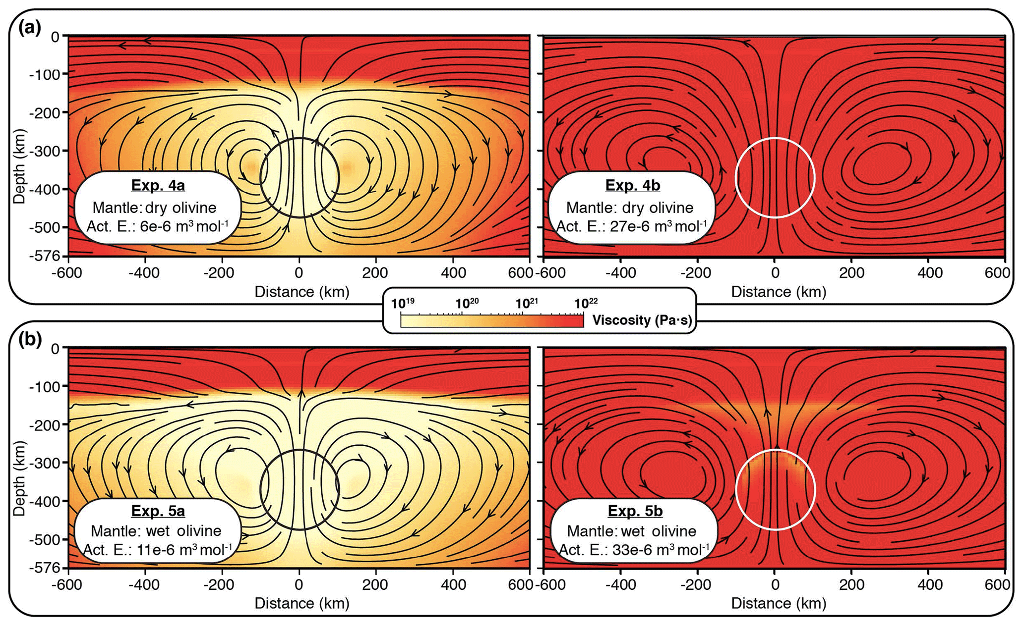
Figure 5 Viscosity map and streamlines for experiments using nonlinear rheologies (dry or wet olivine) with various activation energies. The rising sphere is shown by the circles.

In the case where mantle flow is driven by the temperature difference at the boundary of the convective layer or by internal heating, the dominant strain mechanism is diffusion creep because low deviatoric stresses are expected in the weak convective mantle (Karato and Wu, 1993; Turcotte and Schubert, 2014). However, mantle flow in the vicinity of a moving density anomaly is likely driven by deviatoric stresses that exceed the threshold for dislocation creep. In this case, nonlinear viscosities lead to strong local variation in viscosity. Are those local variations in viscosity important for dynamic topography? To answer this question, we need reasonable constraints on the rheological parameters controlling the viscosity of mantle rocks. However, the extrapolation from laboratory strain rates typically in the range of 10⁻⁶ s⁻¹ to 10⁻⁴ s⁻¹ to mantle conditions where strain rates are typically on the order of 10⁻¹³ s⁻¹ results in significant uncertainties on the activation volume, activation energy and stress exponent (Hirth and Kohlstedt, 2003; Korenaga and Karato, 2008). In what follows, we explore how nonlinear viscosity impacts the dynamic topography and address how the uncertainties on the activation volume can affect dynamic topography.

In Experiments 4 and 5 (Fig. 5), the viscosity depends on temperature, pressure and strain rate as indicated by Eq. (5), using published visco–plastic rheological parameters for the crust and mantle. Specifically, we use quartzite rheology for the crust (Ranalli, 1995), and we test both dry and wet olivine rheologies for the mantle (Hirth and Kohlstedt, 2003). Other parameters are identical to those in Experiments 1–3. We give all the rheological and thermal parameters in Table 1. For a given olivine rheology (i.e. dry or wet) we vary the activation volume by using the minimum and maximum reported values (Hirth and Kohlstedt, 2003).

In the numerical models, the plastic (i.e. brittle) deformation is described via

$$\begin{array}{}\text{(6)}& \mathit{\tau }=\mathit{\mu }{\mathit{\sigma }}_n+C_{\mathrm{0}},\end{array}$$

where τ is the 2nd invariant of the deviatoric stress tensor, which varies with the coefficient of friction (μ), and depth via lithostatic pressure (σ_n), as well as the cohesion (C₀). Due to strain weakening, the cohesion and coefficient of friction decrease from C₀=10 MPa and μ₀=0.577 to C₀=2 MPa and μ₁=0.017 at which the maximum plastic strain (ϵ_max) is reached (i.e. 0.2, Table 1). The effective density (ρ) of rocks is determined by the pressure and temperature using the following equation:

$$\begin{array}{}\text{(7)}& \mathit{\rho }={\mathit{\rho }}_{\mathrm{0}}[\mathrm{1}-\mathit{\alpha }(T-T_{\mathrm{0}}\left)\right][\mathrm{1}+\mathit{\beta }(P-P_{\mathrm{0}}\left)\right],\end{array}$$

where ρ₀, T₀, α and P₀ signify the reference density, reference temperature, thermal expansion coefficient and the compressibility, respectively.

3.2 Numerical results: the case of dry olivine

In Experiments 4a and 4b, we consider dry dislocation creep for olivine (n>1, p=0, r=0). The reported activation volume for this rheology varies between $\mathrm{6}\times {\mathrm{10}}^{-\mathrm{6}}$ and $\mathrm{27}\times {\mathrm{10}}^{-\mathrm{6}}$ m³ mol⁻¹ (Hirth and Kohlstedt, 2003). In Experiment 4a (Fig. 4b), we test the lower value. The streamlines show a similar a pattern to Experiment 2. Interestingly, the maximum vertical velocity peaks at 75 cm yr⁻¹, near the upper boundary of the sphere (Fig. 6a, dashed black line). This is due to the formation of a low-viscosity region above the rising sphere (Fig. 5a, Experiment 4a). This experiment gives a dynamic topography of ∼149 m (Fig. 6b, dashed black line). It confirms that a strong contrast in viscosity between the lithosphere and asthenosphere enhances the dynamic topography signal. We note that the viscosity contrast is attained by smoother transition between the lithosphere and asthenosphere (Fig. 7a, dashed black line). We infer the mechanical thickness of the lithosphere from the viscosity profiles plotted in Fig. 7a, along which the lithosphere–asthenosphere transition zone shows a rapid decrease in viscosity (Conrad and Molnar, 1997). We observe that the effective mechanical thickness of the lithosphere is reduced to 140 km, compared to the thickness of the thermal lithosphere (Fig. 7c).

Figure 6 (a) Vertical velocity profiles (V_y) along the centre and (b) dynamic topography induced by a sphere of temperature anomaly (r=96 km, $\mathit{\delta }\mathit{\rho }/\mathit{\rho }=\mathrm{1}$ %) in the mantle that has nonlinear rheology depending on temperature, pressure and strain rate.

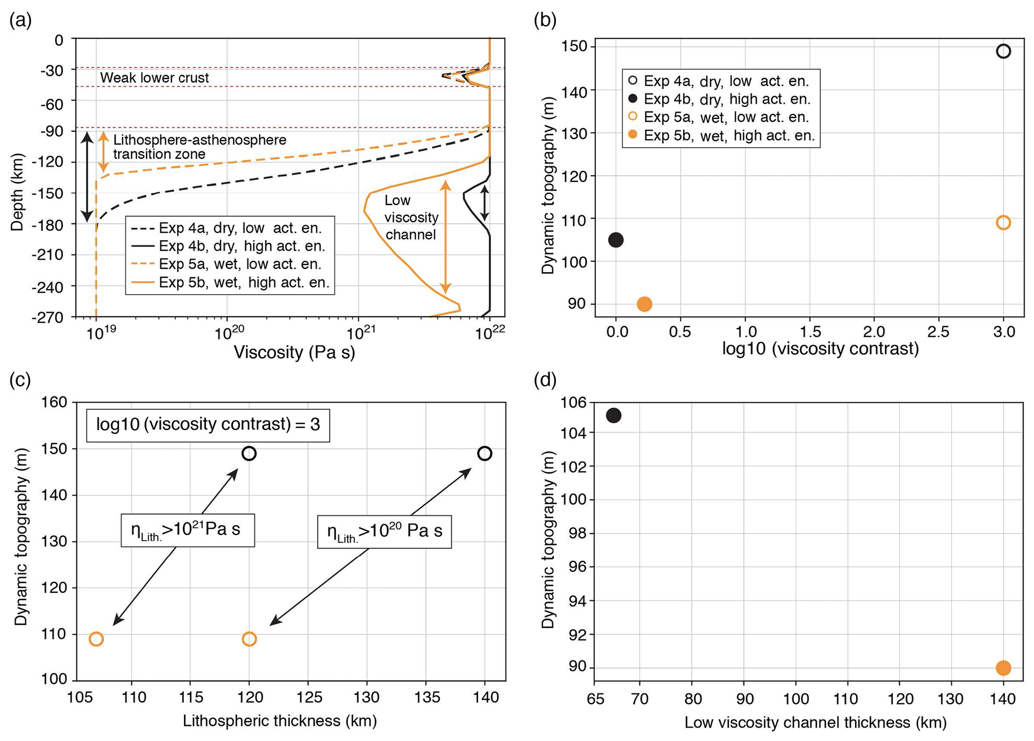
Figure 7 Factors affecting the dynamic topography. (a) Vertical viscosity profiles at the centre of the models. Variation in dynamic topography (b) by viscosity contrast between the lithosphere and part of the asthenosphere above the anomaly, (c) by lithospheric thickness (d) and by thickness of low-viscosity channel.

When we increase the activation volume to $\mathrm{27}\times {\mathrm{10}}^{-\mathrm{6}}$ m³ mol⁻¹, the convection cells grow much larger and show continuity through the lithosphere (Fig. 5a, Experiment 4b). The sphere has a very-low rising speed of ∼ 0.25 cm yr⁻¹ (Fig. 6a, solid black line). Compared to Experiment 4a, the dynamic topography shows a strong decrease from ∼149 to ∼105 m (Fig. 6b, solid black line). This is an example where the system behaves nearly as a single layer with homogenous viscosity. The near absence of viscosity contrast between the lithosphere and asthenosphere explains the smaller magnitude of the dynamic topography. Moreover, the formation of moderately low-viscosity channel (Fig. 7a, solid black line) also contributes to the decrease of the dynamic topography.

3.3 Numerical results: the case of wet olivine

In Experiments 5a and 5b, we consider dislocation creep of wet olivine. The reported activation volume varies between $\mathrm{11}\times {\mathrm{10}}^{-\mathrm{6}}$ and $\mathrm{33}\times {\mathrm{10}}^{-\mathrm{6}}$ m³ mol⁻¹ (Hirth and Kohlstedt, 2003). In Experiment 5a, we test the lower value. The streamlines show a pattern similar to Experiment 4a but with slightly larger convective cells (Fig. 5b, Experiment 5a). The rising velocity of the anomaly exceeds 140 cm yr⁻¹ (Fig. 6a, dashed orange line), promoted by the low-viscosity region sitting above the rising anomaly. The dynamic topography is ∼110 m (Fig. 6b, dashed orange line). This is a bit surprising given the strong contrast in viscosity (3 orders of magnitude) between the lithosphere and asthenosphere. However, Fig. 7a shows that the thickness of the mechanical lithosphere is reduced by about 30 km in comparison to Experiment 4a (e.g. 10 km reduction from thermal thickness) which resulted in lower dynamic topography with similar viscosity contrast (Fig. 7b, c).

In Experiment 5b, we increase the activation volume from $\mathrm{11}\times {\mathrm{10}}^{-\mathrm{6}}$ to $\mathrm{33}\times {\mathrm{10}}^{-\mathrm{6}}$ m³ mol⁻¹. The vertical velocities show significant decrease from 140 to 0.34 cm yr⁻¹ (Fig. 6a, solid orange line). This is due to an increase in viscosity above the rising sphere. Compared to Experiment 5a, the dynamic topography decreases from ∼110 to ∼90 m (Fig. 6b, solid orange line). Compared to Experiment 4b, we expect the dynamic topography to be higher due to slight increase in viscosity contrast (Fig. 7a, b). However, the increase in thickness of the low-viscosity channel (Fig. 7a, d) is more effective and thereby causes a greater reduction in magnitude of the dynamic topography.

In summary, experiments using nonlinear rheology generally give lower amplitudes of dynamic topography compared to experiments using isoviscous rheology (Fig. 8). When we use dry olivine rheology for the upper mantle, the dynamic topography varies between ∼105 and ∼149 m, whereas under wet conditions, the dynamic topography varies between ∼90 and ∼110 m (Fig. 8). These variations are due to uncertainties in the activation volume as well as fluid content in olivine rheologies.

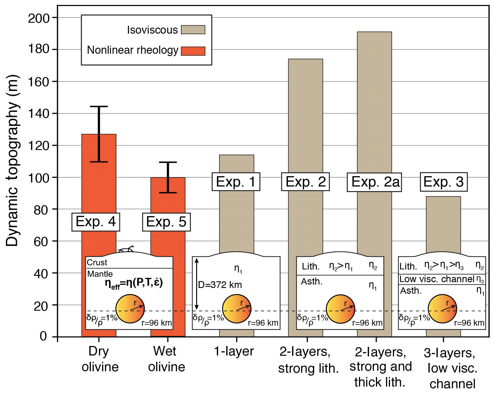
Figure 8 Predicted dynamic topographies driven by a rising sphere centred at 372 km depth with 96 km radius and 1 % less dense than the ambient mantle. The various experiments differ by rheology (isoviscous vs. nonlinear) and viscous structure. For experiments 4 and 5, we show variation in dynamic topography due to contrasting activation energy. In general, experiments with nonlinear rheologies having up to 3 orders of magnitude variation in viscosity generally predict lesser magnitudes of dynamic topography compared to experiments using isoviscous rheology. Compared to dry olivine, wet olivine rheology results in lower dynamic topography.

4 Discussion and conclusion

Using coupled 3-D thermo-mechanical numerical experiments, we have modelled the dynamic topography driven by a rising sphere of 1 % density anomaly, having 96 km radius and emplaced at 372 km depth. In line with analytical studies (Morgan, 1965a; Molnar et al., 2015), the experiments show that dynamic topography is sensitive to viscosity contrast between the lithosphere and asthenospheric mantle, and the thickness of the lithosphere (Fig. 7). Higher viscosity contrasts amplify the dynamic topography (Fig. 7a, b), whereas formation of a low-viscosity channel just below the lithosphere has the opposite effect (Fig. 7a, d). The experiments using nonlinear rheologies show local variations in viscosity, which contribute to the dynamic thinning of the mechanical lithosphere and causes reduction in dynamic topography. In addition, models using high-activation volume creates a low-viscosity channel above the density anomaly, which contributes to decreasing the dynamic topography. Using a larger viscosity range in the models (10¹⁸ Pa s ≤ $\mathit{\eta }\left(PT\dot{\mathit{\epsilon }}\right)\le {\mathrm{10}}^{\mathrm{23}}$ Pa s) resulted in ∼5 % variation in the amplitude of dynamic topography, indicating that the effects of nonlinear rheology are reasonably captured in our models with smaller viscosity range (10¹⁹ Pa s ≤ $\mathit{\eta }\left(PT\dot{\mathit{\epsilon }}\right)\le {\mathrm{10}}^{\mathrm{22}}$ Pa s).

Predictions of dynamic topography derived from mantle convection models are compared against residual topography which is the component of Earth's topography that is not compensated by isostasy (Flament et al., 2013; Hoggard et al., 2016). In a recent work (Cowie and Kusznir, 2018), it has been argued that dynamic topography predictions require scaling of amplitudes by ∼0.75 to match the residual topography, and when density anomalies shallower than 220 km are included, the misfit requires a scaling factor of ∼0.35. It is also important to consider that this misfit depends on the flow wavelength and is suggested to be highest at lowest spherical harmonic degrees (l=2) or very-long wavelengths (Steinberger, 2016). Our numerical experiments show that amplitude of dynamic topography can be nearly halved (e.g. from ∼174 m in Exp. 2 to ∼90 m in Exp. 5b) when we consider nonlinear mantle rheology. Therefore, we propose that, at shorter wavelengths (i.e. less than 1000 km), part of the misfit between the dynamic topography extracted from mantle convection models and dynamic topography estimated from residual topography can be attributed to the Newtonian mantle viscosity used in convection models. If the density sources are shallower, the dynamic topography becomes more sensitive to the viscosity and density structure (Morgan, 1965a; Hager and Clayton, 1989; Osei Tutu et al., 2018), and Newtonian viscosity may lead to higher misfits.

Our models suggest that for shallow density anomalies in the mantle, nonlinear rheologies not only produce lateral variations in viscosity (Richards and Hager, 1989; Moucha et al., 2007) but also additional vertical variations in viscosity that impacts a relatively large area compared to the size of the anomaly in the mantle. We show that this impacts on the thickness of the mechanical lithosphere and predictions of the amplitude of dynamic topography.

As shown in Fig. 8, uncertainties on the activation volume result in variations in dynamic topography which are higher in experiments using dry olivine rheology (i.e. 17 %) compared to experiments using wet olivine rheology (10 %). The comparison between numerical experiments using dry olivine (Exp. 4a) and wet olivine (Exp. 5b) indicates that the variation in dynamic topography can be as much as 25 %. These variations can be lessened if we have better constraints on the mantle rheology, which will advance the dynamic topography models as well as our understanding of the interaction between deep mantle and the Earth's surface.