A new methodology to train fracture network simulation using multiple-point statistics

Natural fracture network characteristics can be establishes from high-resolution outcrop images acquired from drone and photogrammetry. Such images might also be good analogues of subsurface naturally fractured reservoirs and can be used to make predictions of the fracture geometry and efficiency at depth. However, even when supplementing fractured reservoir models with outcrop data, gaps will remain in the model and fracture network extrapolation methods are required. In this paper we used fracture networks interpreted from two outcrops from the Apodi area, Brazil, to present a revised and innovative method of fracture network geometry prediction using the multiple-point statistics (MPS) method.

The MPS method presented in this article uses a series of small synthetic training images (TIs) representing the geological variability of fracture parameters observed locally in the field. The TIs contain the statistical characteristics of the network (i.e. orientation, spacing, length/height and topology) and allow for the representation of a complex arrangement of fracture networks. These images are flexible, as they can be simply sketched by the user.

We proposed to simultaneously use a set of training images in specific elementary zones of the Apodi outcrops in order to best replicate the non-stationarity of the reference network. A sensitivity analysis was conducted to emphasise the influence of the conditioning data, the simulation parameters and the training images used. Fracture density computations were performed on selected realisations and compared to the reference outcrop fracture interpretation to qualitatively evaluate the accuracy of our simulations. The method proposed here is adaptable in terms of training images and probability maps to ensure that the geological complexity in the simulation process is accounted for. It can be used on any type of rock containing natural fractures in any kind of tectonic context. This workflow can also be applied to the subsurface to predict the fracture arrangement and fluid flow efficiency in water, geothermal or hydrocarbon fractured reservoirs.

1 Introduction

1.1 The importance of the prediction of fracture network geometry

Fractures are widespread in nature and, depending on their density and their aperture, might have a strong impact on fluid flow and fluid aquifers (Berkowitz, 2002; Rzonca, 2008), in addition to potentially affecting geothermal (Montanari et al., 2017; Wang et al., 2016) and hydrocarbon reservoirs (Agar and Geiger, 2015; Lamarche et al., 2017; Solano et al., 2010) They are typically organised as networks ranging from the nanometre to the multi-kilometre scale (Zhang et al., 2016), and they present systematic geometrical characteristics (i.e. type, orientation, size and topology) that are determined from specific stress and strain conditions. These conditions have been used to derive concepts of fracture arrangements in various tectonic contexts and introduced the notion of geological fracture-drivers (fault, fold, burial and facies). Based on these drivers, it is possible to some extent to predict reservoir heterogeneity and to define potential permeability pathways within the rock mass (Lamarche et al., 2017; Laubach et al., 2018). Despite the existence of these concepts, a range of parameters including fracture abutment relationships and height/length distributions cannot be adequately sampled along a 1-D borehole and are mainly invisible on seismic images. In addition, fracture networks may present a spatial complexity (variability of orientation or clustering effect) that is also largely unknown in the subsurface. Long and Witherspoon (1985) and Olson et al. (2009) have shown how those parameters impact the connectivity of the network and consequently affect fluid flow in the subsurface. In outcrops, the fracture network characteristics can be observed in 2-D and understood directly. Consequently, outcrops are essential to characterise fracture network attributes that cannot be sampled in the subsurface, such as length or spatial connectivity.

1.2 Surface rocks as multi-scale reservoir analogues

In this context, the study of outcrop analogues is one of the few ways to constrain the architecture of fracture networks (Bisdom et al., 2014; Bruna et al., 2017; National Research Council, 1996; Lamarche et al., 2012; Lavenu et al., 2013). Outcrops can be considered as a natural laboratory where the structural reality can be observed and quantified at various scales. At the small – measurement station – scale (of the order of tens of metres), fracture type, chronologies and topology relationships can be characterised using classical ground-based structural geology methods such as scan lines (Lavenu et al., 2013; Mauldon et al., 2001). At the intermediate – outcrop – scale (of the order of hundreds of metres), the length of fractures and geometry variability can be qualified and quantified using unmanned aerial vehicles (UAVs – drones). Working on outcrops allows for an understanding of the geological history of the target area to be developed and for researchers to decipher how, when and where fractures developed. In addition, outcrops constitute an efficient experimental laboratory where some of properties of the fracture network (i.e. fracture distribution, apertures, permeability and fluid flow behaviour) can be established and modelled (Bisdom et al., 2017a). At the large – reservoir – scale (of the order of thousands to tens of thousands of metres) satellite imagery and geophysical maps provide the characterisation of long objects (hundreds of metres long) such as large fracture systems or faults.

However, not every outcrop can be considered to be a good analogue for the subsurface. Li et al. (2018), in their work on the Upper Cretaceous Frontier Formation reservoir, USA, observed significant differences in the fracture network arrangement in subsurface cores compared with an apparent good surface analogue of the reservoir studied. In the subsurface, fractures appeared more clustered than in the outcrop where the arrangement was undistinguishable from random. The origin of these differences is still debated, but these authors suggest that alteration (diagenesis) or local change in the pressure–temperature conditions may have contributed to the observed variability. The near-surface alteration processes (exhumation and weathering) may also contribute to misinterpretations of the characteristics of the network. In this case, one should be particularly careful when using observed networks to make geometry or efficiency (porosity and permeability) predictions in the subsurface. Therefore, the application of the characteristics observed in the outcrop to the subsurface is not always straightforward or even possible, and may lead to erroneous interpretations. Relatively unbiased signals such as stylolites or veins and particular geometric patterns build trust that the studied outcrop can be compared to the subsurface.

1.3 Modelling approaches classically used to model fracture network geometries

The widely used discrete fracture network (DFN) stochastic modelling tools provide statistical representation of fracture networks generally constrained by a univariate and random distribution of orientation, size, spacing and density/intensity data (Bisdom et al., 2014, 2017a; Huang et al., 2017; Panza et al., 2018). The models generated follow a local stationarity hypothesis. This implies that the statistics used during the simulation are constant in the defined area of interest (Deutsch and Journel, 1997; Gringarten and Deutsch, 1999, 2001; Journel and Zhang, 2006). Liu et al. (2009), highlighted the implicit randomisation that conventional DFN models produce and demonstrated that parameters like fracture connectivity are poorly considered in these representations. In addition, it is generally admitted that discrete realisations of thousands of fracture objects at the kilometre scale are computationally very demanding and often even impossible (Jung et al., 2013). Some authors have attempted to use a pixel-based method to try to predict fracture network geometries. For example, Bruna et al. (2015) used a dense hydrogeological borehole survey sampling a Lower Cretaceous aquifer in the SE of France to define fracture facies and to model their distribution using two-point geostatistics. In this case, the amount of available data and their consistency helped to provide realistic results. However, far from conditioning data (i.e. boreholes) fracture simulation was poorly constrained.

The work of Hanke et al. (2018) used a directional semi-variogram to quantify fracture intensity variability and intersection density. This contribution provides an interesting way to evaluate the outputs of classical DFN approaches but requires a large quantity of input data that are not always available in the subsurface. To represent the fracture network geometry in various geological contexts, an alternative method needs to be developed. This innovative method needs to (i) explicitly predict the organisation and the characteristics of multi-scale fracture objects, (ii) take the spatial variability of the network into consideration and (iii) require a limited amount of data to be realised.

1.4 Multi-point statistics as an alternative to classic DFN approaches

Since Liu et al. (2002), few authors have highlighted the potential of using multi-point statistics (MPS) to generate realistic fracture networks (Chugunova et al., 2017; Karimpouli et al., 2017). Strebelle (2002) showed how MPS are able to reproduce any type of geological heterogeneity of any shape at any size as long as they present a repetitive character. This characteristic seems particularly well adapted to predicting the geometry of a fracture network. The MPS method uses training images (TIs) to integrate conceptual geological knowledge into geostatistical simulations (Mariethoz, 2009). The TI is a grid containing geological patterns that are representative of a certain kind of geological structure, type and arrangement. The TI can be considered as a synthetic model of the geological heterogeneity (i.e. all the elements characterising a geological object) likely to occur in a larger domain (i.e. reservoir, aquifer or outcrop). The TI must contain the range of geobodies that are intended to be modelled, as well as the relationship these geobodies have with one another (Mariethoz, 2009; Strebelle, 2002).

1.5 Objectives and contents of this research

In this paper we propose a MPS workflow considering the geological variability of the fracture network geometry in outcrops (of the size order of 100 m) and a methodology on how to use this method at the reservoir scale. The approach is based on the direct sampling (DS) method (Mariethoz et al., 2010) and uses multiple TIs for a single realisation (Wu et al., 2008). The concept of the probability map has been revised here to define where a training image should be used in the simulation grid. Our outcrop-based simulations also take “seismic-scale” objects (i.e. objects longer than 40 m) into account, which are considered as hard conditioning data. The proposed workflow is tested on outcrops where fracture networks have been previously characterised and interpreted from drone imagery. The outcrops studied are considered as analogues of the Potiguar Basin, Brazil (Bertotti et al., 2017; Bisdom, 2016). Uncertainties were evaluated by comparing original outcrop interpretation (carried out manually by a geologist) with the geometrical characteristics of the network generated from MPS. To evaluate the quality of the simulations, we computed density maps on outcrop fracture interpretation and on selected stochastic models. The proposed approach is innovative and provides a quick and efficient way to represent fracture network arrangements at various scales.

Figure 1 Direct sampling method workflow applied to fracture network modelling (modified from Meerschman et al., 2013).

2 Methodology

2.1 The direct sampling method

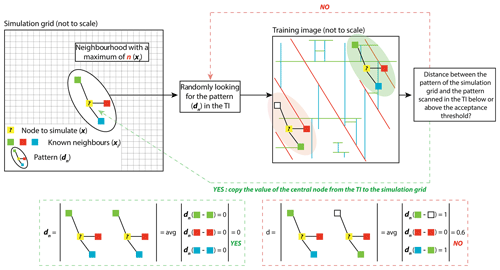
The direct sampling (DS) method was introduced by Mariethoz et al. (2010). Figure 1, synthesises the DS modelling process developed thereafter. The method requires a simulation grid where each node is initially unknown and is referred to as x and a training image grid (TI) where each node is known and referred to as y, i.e. V(y) is defined where V is the variable of interest (e.g. facies value). The simulation proceeds as follows. First, the set of conditioning data (if present) is integrated in the simulation grid. Then, each remaining unknown node x is visited following a random or defined path, and simulated using the following steps. (1) The pattern ${\mathit{d}}_{\mathrm{n}}\left(\mathit{x}\right)=({\mathit{x}}_{\mathrm{1}},V({\mathit{x}}_{\mathrm{1}}\left)\right)$, …, (x_n,V(x_n)) formed by n informed nodes that are closest to x is retrieved. Any neighbour x_i of x is either a previously simulated node or comes from the conditioning data set. The lag vectors ${\mathit{h}}_i={\mathit{x}}_i-\mathit{x}$ define the geometry of the neighbourhood of x. The combination of the value and position of x_i defines the data event or pattern d_n(x). (2) Then, the TI is randomly scanned to search for a pattern d_n(y) similar to d_n(x). For each scan node y, the pattern ${\mathit{d}}_{\mathrm{n}}\left(\mathit{y}\right)=({\mathit{y}}_{\mathrm{1}},V({\mathit{y}}_{\mathrm{1}}\left)\right)$,…, (y_n,V(y_n)), where ${\mathit{y}}_i=\mathit{y}+{\mathit{h}}_i$, is compared to d_n(x) using a distance (Meerschman et al., 2013). When the distance is lower than an acceptance threshold (t) defined by the user or if the proportion of scanned nodes in the TI reaches a maximal fraction (f) defined by the user, the scan is stopped and the value of the best candidate y (the pattern with the minimal distance) is directly attributed to x in the simulation grid (i.e. V(x)=V(y)).

As the DS method does not use a catalogue of all possible patterns found in the TI, it is extremely flexible and allows, in particular, for both categorical and continuous variables and managing multivariate cases to be taken into account, provided that the pattern distance is suitable. In this paper we use the DeeSse version of the direct sampling code (Straubhaar, 2017).

2.2 Multi-scale fracture attributes

To evaluate how the DS method deals with the fracture network, the present experimentation is based on outcrop data where the present-day structural reality is observable at various scales. Pavements (i.e. horizontal surfaces with scales of the order of hundreds of metres) were targeted because they contain important information that is not always accessible with vertical outcrops (Corradetti et al., 2017a, b; Tavani et al., 2016) or with geophysical imagery (e.g. seismic data). The sizes of the pavements allow the user to interpret a large number of fractures and to define areas where the geometry of the network varies (Bruna et al., 2018). Pavements also allow researchers to obtain quantitative data on fracture lengths, which are usually difficult to obtain from vertical cliffs. In the subsurface, data can be provided by geophysical 3-D maps and fracture attribute detection tools (Chopra and Marfurt, 2007; Somasundaram et al., 2017). However, these tools are not always available and only detect the longer lineaments.

Working with pavements constitutes an asset as small-scale investigations can be conducted in key zones of the outcrop (i.e. in folded areas, each compartment or dip domain of the fold should be imaged and investigated in detail where the data gathered will help to calibrate larger-scale information). Classical fieldwork methods (observation and characterisation, measurements, statistical analyses and sampling) help with interpreting fracture families and are essential to constrain larger-scale observations.

In this study, UAV-based photogrammetry is used to obtain an orthorectified mosaic and 3-D digital outcrops models (Bemis et al., 2014; Claes et al., 2017; Vollgger and Cruden, 2016). The scale of these images is an intermediate between the scale of the measurement station and that of the satellite imagery. Digitisation of fracture traces, geological contacts, sedimentary structures and structural domain boundaries are currently processed by hand and represent a considerable time investment. In this contribution, fractures were interpreted in orthomosaic images with the help of GIS software. Length, azimuth, fracture family proportions and fracture density statistics were extracted from the interpretation. In addition, a series of measurement station (area of about 2 m×2 m) information was acquired and compared with the data set from the drone imagery in order to align interpretations and provide coherent fracture history.

2.3 Training images, conditioning data and probability maps

2.3.1 Training images

Training images (TI) are the base input data of the MPS simulation. Building them is a critical step to generate meaningful realisations (Liu et al., 2009). The TI is a pixelated image based on a local interpretation of a geological phenomenon (i.e. an interpreted photograph taken from a local zone of interest in the field) or digitised by a geologist and based on geological concepts (Strebelle, 2002). As the MPS algorithms borrow patterns from the TIs to populate the simulation grid, one should use TIs synthesizing the known geological parameters that characterise the area to simulate. To model non-stationary fields, i.e. fields where the characteristics of the patterns differ depending on their location, one can follow two strategies. The first one consists of using a non-stationary TI containing all the desired spatial features. This requires building one or several auxiliary variables describing the non-stationarity in the TI, and then defining these auxiliary variables in the simulation grid to constrain the simulation. In this way, the auxiliary variable indicates the type of patterns to be simulated in which location (Chugunova and Hu, 2008; Mariethoz et al., 2010; Straubhaar et al., 2011). The second approach consists of using several stationary TIs, each depicting one single type of pattern everywhere. This also requires defining zones in the simulation grid corresponding to each stationary TI (e.g. de Vries, 2009). This second approach is chosen in this work, because it allows for the definition of simple geological concepts (TIs) specific to regions delineated in the simulation domain. The facies proportions and their spatial arrangement are particular to each TI (Figs. 5, 6, 9, 10); therefore, each TI has a local impact on the simulation. Moreover, in our approach, fracture sets are grouped by facies in the TI, based primarily on their orientation and possibly on their length or additional parameters defined by the user. The classification of fractures helps with reproducing patterns and simplifies the process of building the TIs. Note also that two TIs used for two adjacent zones should share some common features in order to obtain realistic transitions between the regions in the simulation domain.

2.3.2 Conditioning data

One limitation of the MPS method is its tendency to disconnect long continuous objects (i.e. typically fractures; Bruna et al., 2017). To manage this issue, long fractures can be identified and incorporated into the simulation as conditioning data. As per the training images, such data can be integrated as pixelated grids. They may come from satellite imagery, or they can be interpreted from gravity or magnetic surveys or from 3-D seismic imagery (Magistroni et al., 2014).

2.3.3 Probability map

The DS method can be used with multiple training images. In this situation, the user provides a set of TIs, and for each TI a probability map is defined on the simulation grid, giving the probability of that TI being used at each node. The pixel-wise sum of these maps should then be equal to one in every node. If each TI corresponds to a partition of the area of interest, with one elementary zone for each TI, covering the whole simulation grid, the probabilities in the map are set to one for specific TIs and to zero for the others.

As per the TIs, the probability map comes from a simple sketch (i.e. a pixelated image) provided by the MPS user. It is based on the geological concepts or interpretations that define the geometry variability over the simulated area and that allow for partitioning of the outcrop. In each of the zones defined in the area of interest, the simulated property will follow the intrinsic stationarity hypothesis (Gringarten and Deutsch, 2001; Journel and Zhang, 2006; Journel, 2005) but the entire domain will be non-stationary.

While working on outcrops, the partitioning of the area of interest can be decided based on observations. For instance, when the fracture network interpreted from outcrop images is available, the geologist can visually define where the characteristics of the network change (fracture orientation, intensity, length and topology) and draw limits around zones where the network remains the same (internal variability; Hooker and Katz, 2015). However, in other cases, outcrops or subsurface observations could be discontinuous between observation sites. If the data are sparse and come mainly from fieldwork ground observations or boreholes, the use of alternative statistical approaches can help to provide a robust and accurate partition of the area of interest. The work of Marrett et al. (2018) interprets the spatial organisation of fractures using advanced statistical techniques, such as the normalised correlation count and the weighted correlation count, on scan lines collected in the Pennsylvanian Marble Falls Limestone. In their approach, the periodicity of fracture spacing (clustering) calculated from the above-mentioned techniques is evaluated using the Monte Carlo method to quantify how different the fracture networks are from a random organisation. These approaches can be highly valuable during the process of building probability maps when limited data are available. The probability maps provide a large-scale framework that may be refined and modified with additional data such as measurement stations or drone surveys from surface exploration or well data containing fracture network information.

2.4 Testing the simulated network: from pixels to segments

MPS realisations are produced as pixelated images. To evaluate the resulting fracture network, pixels' alignments corresponding to fractures are extracted as discrete straight-line objects defined by start and end points. Fractures are separated from the background and are divided into different sets using automatic image classification methods. On grayscale images, this is obtained by multilevel image thresholding via the Otsu method (Otsu, 1979). On colour images, fracture sets are classified based on their colour components via the k-means clustering algorithm built in MATLAB (Lloyd, 1982). Image classification gives a series of binary images as output – one for each fracture set – where lineaments are represented as foreground (Kovesi, 2000).

Figure 2 Locations of the area of interest and of the studied pavements near Apodi (red star).

3 Results: test case on analogues of the Potiguar Basin, eastern Brazil

3.1 Geological setting

The Potiguar Basin is a rift basin located in the easternmost part of the equatorial Atlantic continental margin, north-eastern Brazil (Fig. 2). The basin is found both onshore and offshore (Fig. 2). The basin was generated after the initiation of the South American and African breakup during the Jurassic–Early Cretaceous. It was initially structured by north-west–south-east extension stage that then latterly rotated to an east–west extensional direction (Costa de Melo et al., 2016). The rift basin displays an architecture of horsts and grabens, striking north-east–south-west and is bounded to the east and south by major fault systems (de Brito Neves et al., 1984; Fig. 2). The Potiguar Basin displays three sedimentary sequences deposited since the Early Cretaceous (i.e. syn- and post-rift depositions). The last post-rift sequence has been deposited since the Albian and encompasses the Cenomanian–Turonian Jandaíra Formation. This formation consists of up to 700 m thick bioclastic calcarenites and calcilutites deposited in transgressive shallow marine environment. From the Campanian to the Miocene, the compressive principal stress was oriented north–south (Bertotti et al., 2017). From the Miocene to the Quaternary the onshore part of the Potiguar Basin was uplifted. Synchronously, a new compressive stress field was established trending in a north-west–south-east direction (Reis et al., 2013).

Figure 3 Data acquired in the area of interest from AP3. (a) Orthorectified high-resolution pavement aerial images acquired using a drone; (b) fracture interpretation on orthorectified images; (c) fracture orientation calculated from the north in a GIS-based environment, and the corresponding rose diagram for both outcrops; (d) the length of each fracture trace; and (e) the fracture topology relationship for each pavement observed on fracture network interpretation.

3.2 Outcrop data

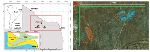
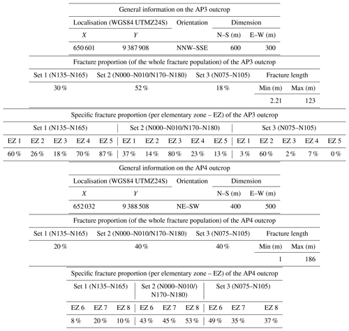
The area of interest measures 2.1 km×1.3 km and is located about 25 km north-east of the city of Apodi in the Rio Grande Do Norte state (Fig. 2). It contains two outcrops AP3 and AP4 (Bertotti et al., 2017; Bisdom, 2016, Fig. 2); here these outcrops are defined as 600 m×300 m and 400 m ×500 m large pavements, respectively, localised in the Jandaíra Formation. AP3 and AP4 crop out as pavements with no significant incision. The outcrops are sparsely covered by vegetation and consequently present a clear fracture network highlighted by karstification. In 2013, images of AP3 and AP4 were acquired using a drone (Bisdom, 2016) and were processed using the photogrammetry method. Two high-resolution orthorectified images of these pavements (centimetre-scale resolution) were used to complete fracture network interpretation and to extract fracture parameters. In AP3, 775 lineaments were traced (Fig. 3), and in AP4, 2593 lineaments were traced (Fig. 4). These lineaments are collectively termed fractures in this paper. For each of these outcrops three fractures sets were identified: Set 1 striking N135–N165; Set 2 striking N000–N010/N170–N180; and Set 3 striking N075–N105. Fractures falling outside of these ranges were not considered in the input data. Consequently, in AP3 we only considered 562 of the 775 fractures traced in the pavement, and in AP4 we only considered 1810 of the 2593 fractures traced. In addition, ground-based fieldwork was conducted on both AP3 and AP4 in order to understand the structural history of the area and to calibrate the interpretation conducted on the drone aerial photography. The general location and fracture data are presented in Figs. 3 and 4 and in Table 1.

Table 1 Outcrop characteristics and fracture parameters collected from AP3 and AP4.

Figure 4 Data acquired in the area of interest from AP4. (a) Orthorectified high-resolution pavement aerial images acquired using a drone; (b) fracture interpretation on orthorectified images; (c) fracture orientation calculated from the north in a GIS-based environment, and the corresponding rose diagram for both outcrops; (d) the length of each fracture trace; and (e) the fracture topology relationship for each pavement observed on fracture network interpretation.

In AP3, sets 1 and 2 are distributed over the pavement. However, their intensity is variable in the area of interest. Set 3 is mainly expressed in distinct regions of the outcrop. Small-scale investigations (conducted on measurement stations in the outcrop) showed that Set 3 is composed of stylolites, and sets 1 and 2 are composed of veins. In addition, sets 1 and 2 present evidence of shear movements and are then considered as a conjugate system.

In AP4 small-scale investigations highlight the same characteristics as those observed in AP3. Although the conjugate system (Set 1 and Set 2) is less developed there than in AP3. It is also notable that more cross-cutting relationships were observed in AP4 than in AP3.

3.3 Input data for MPS simulation

To evaluate the effect of conditioning data, results of two simulations were compared, with and without conditioning data. The sensitivity of the simulation parameters was investigated by varying (i) the number of neighbours defining patterns (data events d_n), (ii) the acceptance threshold (t) defining the tolerance that the algorithm authorises to find a matching data event in the simulation grid (Mariethoz et al., 2010) and (iii) the fraction of the TI to be scanned during the simulation process to search for data events. Results of this sensitivity analysis help to propose the best possible simulation for AP3 and to optimise the choice of input parameters for the AP4 fracture simulation.

AP3 presents intrinsic fracture network geometry variability. This observation emphasises that averaging fracture parameters over the entire domain is not well suited to represent the complexity of the network. We observed that the length of the fractures per set and the density of fractures are parameters that vary the most here. The analysis of these variations allow the user to partition AP3 and AP4 in elementary zones and to synthesise the fracture network characteristics in each of these domains. The following section defines how the TI, probability map and conditioning data were built.

3.3.1 Partitioning, training images and probability maps for AP3 and AP4

We divided AP3 into five elementary zones (EZ) based on visual inspection of the pavement (Fig. 5a, b). The number of fractures per EZ is synthesised in Fig. 5. The proportion of fractures per elementary zone is available in Table 1. A limited part of the fractures belongs to two adjacent elementary zones. This issue is quantified in Table 1.

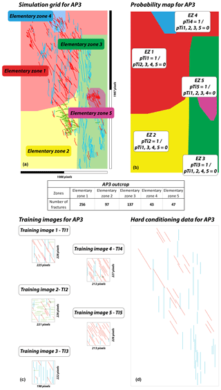
Figure 5 (a) Partitioning of AP3 into five elementary zones (EZ). This partition is defined with respect to fracture orientation (which in this case defines the fracture facies), fracture density and geometry variability over the entire simulation domain. (b) Probability map and associated statistics for each EZ. (c) Training images associated with the partition of AP3. In each EZ, the corresponding training image has a probability (pTI) of one of being used. In this zone the other training images are not used (pTI =0). (d) Hard conditioning data for AP3. All of the fractures longer than 40 m are considered deterministically in the simulation process.

A probability map with sharp boundaries (Fig. 5b) was created for AP3. Sharp boundaries are justified by the variability of the network geometry, which is known from the visual inspection of the interpreted image. Smooth transitions could also be defined (see discussion). The input data used to build the probability map is an image of the partition of the area of interest containing the different outcrops. In this image, the indexed zones (elementary zones, EZs) are characterised using distinct colours.

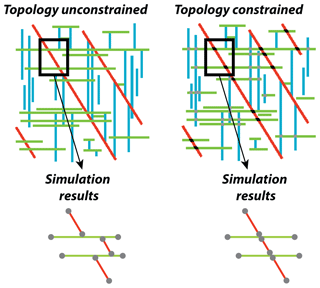
At the reservoir-scale, where some outcrops analogues and fracture tracing may be available, the interpreted reality of the network (e.g. a binary fracture/non-fracture image) can be directly used as a training image. We chose to ignore the tracing and to rely on parameters that are attained through field observation without having access to drone images of an entire outcrop (i.e. orientation, spacing and abutment) and to compare the interpretation with the simulated network. In that respect, fracture orientations were averaged to a single value. Hence, Set 1 strikes N090, Set 2 strikes N150 and Set 3 strikes N180. According to the outcrop partitioning, five training images were created (Fig. 5c). In each training image, three facies corresponding to the three fracture sets were created. Set 1 is green, Set 2 is red and Set 3 is blue (Fig. 5c). The topology is a crucial problem in fracture simulations because it influences the connectivity of the network. In the MPS simulations the abutments are particularly well reproduced as they represent singular pixels' arrangements which are efficiently taken into account. However, cross-cutting relationships imply the use of a different facies at the intersection locus. This method respects and reproduces intersections during the simulation process. In AP3, the analysis of the topology relationships showed three main cross-cutting interactions:

• Long fractures from Set 2 and long fractures from Set 3 mutually cross-cut (conjugated sets);

• Set 3 cross-cut Set 1; and

• Set 2 cross-cut Set 1

To take these topological parameters into account a different facies colour was attributed to the cross-cutting locus (the crossing facies, Fig. 6). When the MPS realisation is later discretised, the younger fractures will be truly represented as continuous segments. The older fractures will be cut into pieces, but their alignment will be (in most cases) maintained during the simulation process.

Figure 6 Comparison between results obtained without constraining the topology and those obtained with topological facies constraints.

3.3.2 Dimensions of the simulation grids and of the training images

The dimensions of the simulation grid for AP3 and of each training image (in pixels) are shown in Fig. 5. The number of pixels is automatically determined by the size of the original drawing made by the geologist.

The size of the input training image does not generally influence the simulation. However, it has to be large enough with respect to the complexity of the patterns in order to obtain reliable spatial statistics. The DS method tends to identify patterns (i.e. d_n values; see above) in the TI and to paste the central node of them into the simulation grid. However, at a constant resolution and specifically for fracture patterns, it is likely that a 50 m ×50 m training image will carry more complexity and variability than a 10 m ×10 m image. This parameter should be taken into consideration when starting to digitise training images, especially when spacing between fractures is not consistent across the simulation grid.

3.3.3 Long fractures conditioning

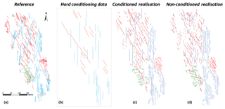
Because the MPS method has the tendency to cut long individual segments into smaller pieces, the fractures longer than 40 m – those visible from satellite/drone imagery in AP3 – were isolated and considered to be hard conditioning data (Fig. 5d). This threshold was arbitrarily determined from the data set we had. In AP3, less than 8 % of the fractures were longer than 40 m.

In AP3, long fractures only belonged to the sets oriented/striking N180 or N150 (Fig. 5d). A total of 18 N180 fractures (3 %) and 30 N150 fractures (5 %) were digitised and integrated as conditioning data in the simulation.

Figure 7 Visual comparison between (a) the reference fracture network interpretation (AP3), (b) the extraction of the longer segments (50 fractures longer than 40 m), (c) a simulation conditioned by the long segments and (d) a simulation not conditioned by the long segments.

4 Outcrop-scale simulations

4.1 Impact of conditioning data on AP3 simulations

In AP3, the 48 long fractures were manually digitised and imported into the simulation grid as categorical properties to be considered as hard conditioning data during the MPS simulation process. Consequently, the MPS simulation is in charge of stochastically populating the smaller fractures within the grid.

Results of the influence of these data are presented in Fig. 7. The principal simulation parameters in the scenarios considered (with and without conditioning data) were set up identically: constant acceptance threshold (5 %), constant percentage of scanned TI (25 %) and constant number of neighbours (50).

Results showed that the realisation without conditioning data creates 20 % less fractures than the original outcrop reference. The simulation with conditioning data creates 9 % less fractures than AP3, which allows for better replication of the long fracture than a non-conditioned simulation. It is also remarkable that the non-constrained simulation represents only 23 fractures above 40 m (compared with the 48 long fractures interpreted on the AP3 outcrop). In this simulation the long fractures are essentially located in the zone 3 of the outcrop. Because the simulation is a stochastic process, the location of the long fractures is randomly determined in the absence of hard conditioning data. This is considering that hard-conditioning data also give a more realistic representation of the fracture network.

4.2 Sensitivity analysis on the AP3 simulation parameters

4.2.1 Simulation parameter set-ups, duration and analyses conducted on the results

Simulation parameters were varied for each simulation in order to emphasise their effect on each realisation. One realisation per test was performed during this analysis. The goal of this analysis was to show how the different parameters influenced the reproduction of fracture segments and not to evaluate how good the agreement between the simulation and the reference was.

The MPS realisations are pixelated images. The sensitivity analysis is based on the discrete segments extracted from these pixelated images (see Sect. 2.4). All of the simulations present a variable percentage of segment lengths that are below the minimal fracture length interpreted in the AP3 outcrop (i.e. simulation noise). Consequently, all segments smaller than 2.2 m where removed from the simulation results. A length frequency distribution was compiled for each of the simulations generated.

Table 2 Simulation parameterisation, model set-ups and duration (in seconds) of each run. In the table A. th. stands for acceptance threshold, N stands for number of neighbours and “Scan” denotes the scanned fraction of the training image.

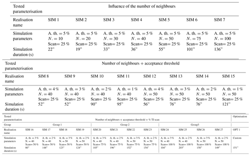
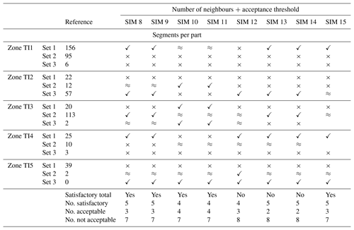
The influence of the number of neighbours was evaluated via seven simulations (SIM 1–SIM 7). The acceptance threshold and the number of neighbours was investigated by comparing eight simulations (SIM 8–SIM 15) where the scanned fraction of the TI was fixed at 25 %. The percentage of the scanned fraction of the TI was combined with the two other simulation parameters. This combination was tested over 12 simulations (SIM 16–SIM 27). The model set-ups and the durations of the simulations are presented in (Table 2). It is notable that SIM 8/SIM 9, SIM 10/SIM 11 and SIM 13/SIM 14 produce exactly the same network despite the modification of the simulation parameters. Furthermore, the MPS algorithm successfully performed SIM 16, but the segment extraction generated an error preventing the discretisation of all of the objects.

Table 3 Comparison between the total amount of segments interpreted in the reference outcrop and in the different sets of simulations (tested parameterisation). Evaluation of the results in terms of satisfactory (✓), acceptable (≈) or non-satisfactory (×).

The total amount of generated fractures segments was counted and compared with the total amount of fracture traces interpreted from the original outcrop. A deviation of 10 % compared with the original number of fractures interpreted was considered as a satisfactory result, as it is very close to the reference number of fractures. A deviation of 20 % compared with the original number of fractures interpreted was considered to be an acceptable result. This deviation is consequent but can be adjusted by varying the simulation parameters. A deviation above 20 % was rejected, as a complete reconsideration of the parameters is required. Results are synthesised in Table 3.

The total number of segments was initially counted over the entire simulation domain. The sum of segments per part is constantly higher than the initial total number of segments because segments cutting a sharp boundary are divided in two – segments falling within two elementary zones and are consequently counted twice. The number of fractures generated per simulation zone was also computed, and the same deviation thresholds were applied to evaluate if the simulation was satisfactory, acceptable or rejected. Tables 4 to 6 synthesise the sensitivity analysis conducted for 27 realisations of the AP3 outcrop.

The length of the segments were computed for each realisation and are presented in Fig. 8.

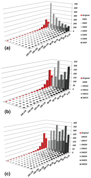
Figure 8 Fracture length distributions tested during the sensitivity analysis. (a) Fracture length distribution for SIM 1–SIM 7, (b) fracture length distribution for SIM 10, SIM 12, SIM 13 and SIM 15, and (c) fracture length distribution for SIM 16, SIM 17, SIM 20, SIM 21, SIM 22, SIM 24, SIM 5 and SIM 26. The x axis represents the lengths of the classes of fracture in metres, and the y axis represents the number of fracture per length class.

The influence of the hard conditioning data and of the drawing of the training image was also quantitatively investigated and compared with the length of the generated segments and with the amount of segments generated per zone respectively.

4.2.2 Summary of the results

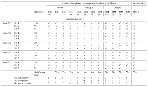
Increasing the number of neighbours lengthens the computation time (Table 2, SIM 1–7). A small number of neighbours results in a noisy simulation (Table 2, SIM 1). The contrary leads to a downsampling of the generated segments that become longer than the fractures interpreted in AP3 (Table 2, SIM 7). Decreasing the acceptance threshold leads to an increase in the simulation time (Table 2, SIM 8-15). Increasing the scanned fraction of the TI is the most time consuming operation (Table 2, SIM 17–27).

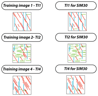
Figure 9 Comparison of training images 1, 3 and 4 used during the sensitivity analysis (27 simulations) and their modification for SIM 3.

Increasing the number of neighbours only is generally not sufficient to accurately generate a satisfactory or acceptable total number of fractures (Table 3). Increasing the scanned fraction of the TI produces the closest total number of fractures compared to the reference outcrop in all cases (Table 3).

Table 4 Results of the sensitivity analysis on the influence of the number of neighbours. The table presents the number of segments per simulation zone for AP3 (used as a reference). × show a total number of segments of the considered set in the considered zone deviating by more than 20 % from the reference case. ≈ show a deviation of more than 10 % from the reference case. ✓ do not deviate significantly from the reference outcrop interpretation.

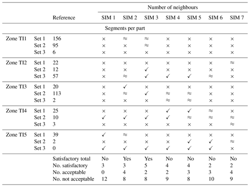
The counting of fractures in simulation zones revealed that Set 2 and Set 3 in zone 1, Set 3 in zone 4 and Set 1 in zone 5 are generally underestimated during the simulation process. In contrast, fracture Set 1 in zone 2 is generally overestimated. The consistency of the error over almost the entire set of simulations indicates an issue with the training image representation (Tables 4–6). Increasing the scanned fraction of the TI generally allows for a better representation of a low proportion of fracture facies within a TI (zone TI5, Set 2; Table 6).

An acceptance threshold below 5 % leads to an overestimation of the number of small fractures (between 0 and 10 m), Fig. 8. In this case, the number of segments between 0 and 20 m is generally close to reality. Increasing the scanned fraction of the TI produces the highest quantity of fractures ranging from 0 to 10 m (Fig. 8). Increasing the number of neighbours and the percentage of the scanned TI results in an increase of the length of the fractures used as hard conditioning data. However, the fracture elongation does not affect all of the hard conditioned fractures and represents a very small percentage of the whole modelled fracture network.

Table 5 Results of the sensitivity analysis on the influence of the number of neighbours and on the variation of the acceptance threshold. The symbols are the same as those used in Table 4.

4.3 Attempt at an optimisation: OPT1

OPT1 was parameterised with respect to the previous observations in order to generate a simulation that is as close as possible to reality. For this purpose, the number of fractures from Set 2 and Set 3 drawn in TI1 and Set 3 drawn in TI4 was increased. In contrast, the number of fractures from Set 1 drawn in TI2 was decreased significantly (Fig. 9). We choose to set the number of neighbours at 50 and set the acceptance threshold at 2 %. TI1 and TI4 were scanned at 75 % and the rest of the TIs were scanned at 50 % (Table 2).

The simulation time for the proposed simulation was 2 min 31s (Table 2). The total number of fractures generated was satisfactory compared with the number of fractures interpreted in the original outcrop.

To evaluate the robustness of the optimised simulation, six realisations using the same parameterisation were generated for OPT1. The total number of fractures generated for these simulations always fell below the 10 % deviation compared with the reference outcrop.

The number of segments comprised between 0 and 20 m in OPT1 was slightly above the satisfactory deviation limit. As per all of the simulations generated, the number of fractures between 2.21 and 10 m was largely overestimated.

OPT1 contained a more satisfactory and acceptable fracture count than previous simulations (Table 6). The number of segments generated in zone 1 and 2 for Set 1 was slightly overestimated. In zone 3, OPT1 failed to represent the amount of fractures for Set 1 (25 % deviation) and for Set 3. Fracture Set 1 in zone 4 was largely overestimated.

Figure 10 Comparison of the fracture intensity (P₂₁) calculated in the reference outcrop and in four select MPS simulations.

4.4 Evaluation of the AP3 and OPT1 simulations: P₂₁ calculations

Uncertainty analysis is required when performing simulations of geological parameters, especially far from data. The sensitivity analysis presented in this paper is a way to compare the MPS simulations with the reference outcrop.

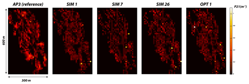
To reinforce the evaluation of the proposed method, we quantified the values of fracture intensity in the reference outcrop and in three selected AP3 MPS simulations and the optimised simulation (OPT1; Fig. 10). The fracture intensity was classified as in Dershowitz and Herda (1992) with regard to (i) the size and dimension (1-D, 2-D or 3-D) of a selected zone of interest and (ii) the number, length, area or volume of fractures within this selected zone. In this paper, we chose to calculate the P₂₁ fracture intensity, which corresponds to the sum of all fracture lengths within a regularly discretised space, with constant area boxes (10 m ×10 m) covering the entire AP3 area of interest.

Table 6 Results of the sensitivity analysis on the influence of the number of neighbours, of the variation of the acceptance threshold and of the variation of the percentage of the scanned fraction of the training image. The symbols are the same as those used in Tables 4 and 5.

Visually, the results show an apparent higher P₂₁ intensity in the reference outcrop than in the simulations. However, zones of high intensity in the reference outcrop are generally well represented in SIM 26 and in OPT1. This is in agreement with the results of the sensitivity analysis showing that SIM 26 and OPT 1 best represent the number of fractures present in the reference outcrop.

The average fracture intensity in each simulation was also computed and confirmed the observations conducted during the sensitivity analysis. SIM 1 and SIM 7 presented the lowest average fracture intensity (0.095 and 0.079 m⁻¹ respectively) and SIM 26 and OPT 1 presented the highest fracture intensity (0.11 and 0.099 m⁻¹ respectively). The average fracture intensity in the reference outcrop was higher than in any other simulations (0.126 m⁻¹). However, this value remained close to those obtained in SIM 26 and OPT 1.

The fact that the fractures were simplified as straight lines in the simulations combined to a relatively small area of calculation (10 m ×10 m) could be one element explaining the observed fracture intensity variation between the reference outcrop and SIM 26 and OPT 1. This analysis strengthens the results obtained during the sensitivity analysis and demonstrates the capacity of the MPS method to represent the geometry of a fracture network with a high fidelity .

Figure 11 (a) Partitioning of AP4 in three EZs. (b) Probability map and associated statistics for each EZ. (c) Training images associated with the partitioning of AP4. (d) Hard conditioning data for AP4.

4.5 Using the sensitivity analysis results to model AP4

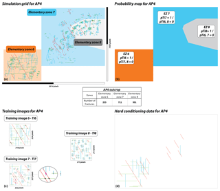
As per AP3, AP4 presents an intrinsic variability of the fracture network geometry. This outcrop was divided in three elementary zones (Fig. 11a, b). According to AP4 partitioning, a probability map with sharp boundaries (Fig. 11b) was created. For AP4, the configuration of the outcrop led to masking the area where no interpretation data were performed. In these particular zones, a “no data value” was attributed and these masked areas were excluded during the modelling process. In AP4 three training images were created (Fig. 11c). As per AP3, the size of the AP4 simulation grid was doubled compared with its original dimension (available in Fig. 11). In AP4, fractures longer than 40 m were also considered to be hard conditioning data. Here, less than 1.5 % of the fractures were longer than 40 m (Fig. 11d). In AP4, long fractures were found in the three sets and mainly in the south-eastern part of the outcrop (Fig. 11d, “Elementary zone 6”). A total of 11 N180 fractures (0.5 %), 13 N150 fractures (0.6 %) and 9 N090 fractures (0.4 %) were digitised and integrated as conditioning data into the simulation.

Figure 12 Comparison of the AP4 original outcrop with a MPS simulated version AP4-1.

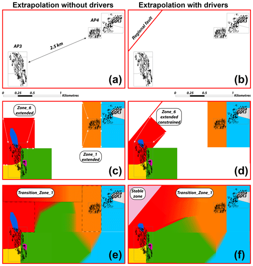
Figure 13 Smooth probability map at the reservoir scale (combination of AP3 and AP4). (a) Relative position of the AP3 and AP4 outcrops. (b) Apodi fault added into the area of interest. Extension of the probability map regions in AP3 and AP4 without geological drivers (c) and with the influence of the Apodi fault (d). Probability maps with smooth transition zones without geological drivers (e) and with the influence of the Apodi fault (f).

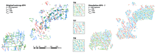
Based on the results of the sensitivity analysis of AP3 we generated one simulation for the AP4 outcrop (Fig. 12). The modelling parameters for SIM AP4-1 were selected as follows: the number of neighbours was set at 50 and the acceptance threshold was set at 2 %. The three training images used in the simulation are presented in Fig. 12 and were considered as representative of the fracture arrangement in each region of the simulation. The scanning percentage of TI6 and TI7 was set at 50 %. The scanning percentage of TI8 was set at 100 %. With this configuration, the simulation lasted slightly more than 5 min. The process of intensely scanning TI8 was probably responsible for this duration. The analysis was conducted on the total number of segments generated and on the segments per set of fractures. In AP4 the total number of segments was 1810. The simulation realised 1682 segments in total, which constitutes a satisfactory result. The original AP4 simulation presented 252 segments striking N150, 856 segments striking N180 and 702 segments striking N090. The results of the AP4-1 simulation were always satisfactory or acceptable with 206 segments striking N150, 834 segments striking N180 and 642 segments striking N090. A detailed analysis was not conducted here because AP4 contained a lot of small fracture intersections (especially in the TI8 zone) and this made the segment extraction a complex process. However, these results are promising for the future.

5 Smooth transitions between elementary zones: towards reservoir-scale models to manage uncertainties

The strength of the method proposed here relies on the use of probability maps and on considering multiple training images in a single realisation to generate non-stationary models of fracture network geometries. In the cases of AP3 and AP4, the probability maps were essentially constrained by the variation of the geometry of the fracture networks observed on the geological interpretation made on the drone imagery. Consequently, the defined areas are pragmatically bounded and the nature of the limit between one zone and another is a sharp boundary.

The AP3 and AP4 outcrops are separated by about 2.5 km and very little is known about the fracture network geometry between these two locations. Assuming that there is no major structural deformation (fold or faults) that may cause a change in the fracture geometry in close vicinity to the outcrop “reality”, the zones initially defined on the AP3 and AP4 outcrops can be extended to the limits of the reservoir-scale model boundaries (Fig. 13). In this particular case, filling the gap between the two outcrops appears to define how the transition between one side of the simulation grid and the other should be determined.

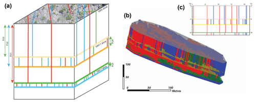
Figure 14 Fracture network extrusion in 3-D. The method consists of identifying the different fracture units (FU) on which the fracture height is supposed to be constant (a). This method requires one simulation per top fracture unit (SIM slices). (b) A 3-D DFN based on the hypothetical case (a) and realised in GOCAD software. (c) A cross section realised in the centre of the 3-D model in the east–west direction.

Fractures are localised objects that do not need to be necessarily continuous from one simulation zone to another. The constant higher proportion of the non-fractured matrix facies versus localised and thin fracture elements ensures the coherency and relative compatibility from one simulation region to another. The idea of the simulation grid region partitioning was re-evaluated, and an alternative method was proposed here. Contrary to the definition of sharp boundaries in the probability maps used for AP3 and AP4, a probability map with smooth transitions is defined as follows. An ensemble of elementary zones covering a part of the simulation grid is defined. Each TI corresponds to one elementary zone, which is simulated exclusively using that TI. The probabilities in these zones are then set to one for a specific TI and to zero for the others. The remaining part of the simulation grid is divided into transition zones, for which one has to define which TIs may be involved. In a transition zone, the probabilities of the TIs involved are set to be proportional to the inverse distance to the corresponding elementary zones. This process creates smooth transitions in poorly constrained areas, decreasing the influence of one TI on another (from one elementary zone to another).

No faults or folds can initially be identified between AP3 and AP4 to condition the drawing of the probability map. In this case, a rectangular compartment representing a gradual probability transition to the use of a training image associated with one outcrop or another filled the blank space between the two outcrops. For instance, in “Transition_Zone_1”, Fig. 13e shows a decreasing probability of the use of TI1 from left to right (i.e. zone 1 to zone 6) and conversely of the use of TI6 from right to left.

Recently, investigations conducted on the Rio Grande do Norte geological map (Angelim et al., 2006) have demonstrated the presence of a fault crossing the simulation grid near the AP3 zone. This structure may explain the variability of fracture geometry from AP3 (east–west stylolites and the strong presence of a conjugated north–south/north-west–south-east system) to AP4 (east–west stylolites associated with a north–south fracture system; the north-west–south-east conjugated system is subordinate here). Further geological investigations need to be conducted in this particular location to examine the influence of this fault on the network geometry. However, Fig. 13f shows an alternative probability map taking this interpretation into account and shows how flexible the probability map can be. The proposed method demonstrates its adaptability in various geological contexts.

6 A method to create a 3-D DFN from 2-D MPS realisations

The MPS simulations presented in this paper are in the form of 2-D pixelated maps. MATLAB codes were developed to extract start and end point coordinates (georeferenced) of a series of aligned, colourised pixels that represent a fracture trace from these images. Transforming this output into geologically realistic 3-D surfaces is not easy. Karimpouli et al. (2017) studied samples from coal bed methane reservoirs in the fractured Late Permian Bowen Basin in Australia. They realised multiple 2-D and pseudo-3-D images (i.e. orthogonal 2-D images) and used cross-correlation based simulation (CCSIM) to represent the internal organisation of coal cleats and the heterogeneity of the coal matrix in 3-D. Their approach greatly improved the understanding of the internal complexity of coal samples and gives better results than classical DFNs based on averaged distributions. However, their method requires an important amount of initial information (i.e. CT scan slices used as training images) which is generally not available at a larger scale. The use of MPS in 3-D seems particularly unsuited for fracture network representation due to the following: (i) they require the association of fractures from a 2-D map view and from a 2-D section view (3-D or pseudo-3-D); (ii) it appears difficult to consider isolated fractures using this type of approach; and (iii) in the subsurface fracture height and/or fracture length are generally unknown.

To tackle these problems we chose to use multiple 2-D MPS-generated fracture networks. In the presented approach, the 3-D image is obtained by extruding 3-D fracture planes in fracture units (Fig. 14). In this approach we consider that fractures are entirely bound to the units, which can appear as a limitation if isolated fractures occur inside a layer. However, we can consider variable levels of fracture units. Figure 14 presents an hypothetical scenario where red fractures are confined to a large fracture unit (FU1) cross-cutting smaller ones (FU4 also contains smaller red fractures). In a representation such as this, one 2-D planar simulation is required at each top mechanical unit to generate a new set of fractures.

In real-world subsurface configurations, mechanical units can be extracted from well logs (resistivity, density and lithology; Laubach et al., 2009). The fracture height distribution, referred to as the fracture stratigraphy (Hooker et al., 2013) requires particular attention here and is difficult to extract from borehole data. With respect to outcrops, the use of vertical cliffs adjacent to 2-D horizontal pavement may be a way of evaluating these heights and constraining the 3-D model.

In outcrops, resorting to vertical cliffs adjacent to 2-D horizontal pavements is required to define fracture height. This method is already implemented in SKUA-GOCAD software as a macro that extrudes planes of a single fracture family (i.e. all of the red fractures in AP3) vertically into a bounded volume (Fig. 14). More developments are currently in process to generate oblique planes and to be able to extrude planes in portions of the fracture sets.

7 Conclusions

In this paper a new method for predicting the geometry of a natural fracture network using the multiple-point statistic algorithm is presented. The method provides a stochastic realisation depicting a realistic non-stationary fracture network arrangement in 2-D based on the use of multiple, simplified, small training images capturing the natural fracture attributes in specific zones defined by a probability map. Probability maps are adaptable and follow the geological rules of fracture type and arrangement distribution specific to various tectonic contexts (i.e. faulting, folding and poor deformation context/no fault, no folds). We developed methods to be able to consider transition zones in probability maps (e.g. zones far from hard data) which allow for the simulation of fracture network geometry at a larger scale (i.e. reservoir scale).

The realisations obtained from 2-D MPS constitute a statistical laboratory close enough to reality to be tested in terms of fracture mechanical parameters and response to flow.

The method proposed here is applicable to all rock types and to a wide range of tectonic contexts. Initially calibrated using outcrop data, the method is fully adaptable to the subsurface in order to better characterise fractures in water, heat or hydrocarbon reservoirs. However, the challenge there is the definition of the different training images on which the simulation is based. Very few data are generally available in the subsurface, and geological rules need to be found to define the geological characteristics of the fracture network (orthogonal or conjugate network) and the associated fracture attributes (length, height, spacing, density and topology).

Appendix A

The DeeSse algorithm (Straubhaar et al., 2011) was used in this paper to reproduce existing fracture networks interpreted from outcrop pavements. The following pseudo-code developed by Oriani et al. (2017) has been modified to explain how the algorithm processes the simulation of fractures. Specific terms can be found in Sect. 2.1 of this paper. In our study, the simulation follows a random path into the simulation grid. This grid is populated by values (fracture facies in our case) according to the following sequence:

1. The selection of a random location x in the simulation grid that has not yet been simulated (and does not correspond to conditioning data points that have already been inserted in the grid).

2. To simulate V(x), the fracture facies, into the simulation grid, the pattern ${\mathit{d}}_{\mathrm{n}}\left(\mathit{x}\right)=({\mathit{x}}_{\mathrm{1}},V({\mathit{x}}_{\mathrm{1}}$)),…, (x_n,V(x_n)) formed by n informed nodes that are closest to x is retrieved. If no neighbours are assigned (at the beginning of the simulation), d_n(x) will then be empty; in this case, the value V(y) of a random location y in the TI will be assigned to V(x), and the procedure will be repeated from the beginning.

3. A random location y in the TI is visited and the corresponding data event d_n(y) is retrieved.

4. dn(x) is compared to d_n(y) using a distance D(d_n(x),d_n(y)) corresponding to a measure of dissimilarity between the two data events.

5. If D(d_n(x),d_n(y)) is smaller than a user-defined acceptance threshold T, the value of V(y) is assigned to V(x). Otherwise step 3 to step 5 are repeated until the value is assigned or a given fraction F of the TI is scanned.

6. If F is scanned, V(x) is defined as V(y) with y, the scanned location, minimising the distance D(d_n(x),d_n(y)).

7. The whole procedure is repeated until the whole simulation grid is informed.