the Creative Commons Attribution 4.0 License.
the Creative Commons Attribution 4.0 License.
 | 29 Apr 2019
The cross-dip correction as a tool to improve imaging of crooked-line seismic data: a case study from the post-glacial Burträsk fault, Sweden
Ruth A. Beckel
Christopher Juhlin
Understanding the development of post-glacial faults and their associated seismic activity is crucial for risk assessment in Scandinavia. However, imaging these features and their geological environment is complicated due to special challenges of their hardrock setting, such as weak impedance contrasts, often high noise levels and crooked acquisition lines. A crooked-line geometry can cause time shifts that seriously de-focus and deform reflections containing a cross-dip component. Advanced processing methods like swath 3-D processing and 3-D pre-stack migration can, in principle, handle the crooked-line geometry but may fail when the noise level is too high. For these cases, the effects of reflector cross-dip can be compensated for by introducing a linear correction term into the standard processing flow. However, existing implementations of the cross-dip correction rely on a slant stack approach which can, for some geometries, lead to a duplication of reflections. Here, we present a module for the cross-dip correction that avoids the reflection duplication problem by shifting the reflections prior to stacking. Based on tests with synthetic data, we developed an iterative processing scheme where a sequence consisting of cross-dip correction, velocity analysis and dip-moveout (DMO) correction is repeated until the stacked image converges. Using our new module to reprocess a reflection seismic profile over the post-glacial Burträsk fault in northern Sweden increased the image quality significantly. Strike and dip information extracted from the cross-dip analysis helped to interpret a set of southeast-dipping reflections as shear zones belonging to the regional-scale Burträsk Shear Zone (BSZ), implying that the BSZ itself is not a vertical but a southeast-dipping feature. Our results demonstrate that the cross-dip correction is a highly useful alternative to more sophisticated processing methods for noisy datasets. This highlights the often underestimated potential of rather simple but noise-tolerant methods in processing hardrock seismic data.
- Article
(24320 KB) - Full-text XML
-
Supplement
(2014 KB) - BibTeX
- EndNote


Today, northern Scandinavia is generally considered to be a low seismic hazard area. There are a number of intraplate earthquakes connected to the post-glacial rebound, but only very few of them exceed a magnitude of 4 (Bödvarsson et al., 2006). In the past, however, the post-glacial adjustments seem to have been more intense. Throughout northern Scandinavia, up to 15 m high fault scarps extending for tens of kilometers (Fig. 1) suggest the occurrence of violent earthquakes at the end or directly after the last glacial retreat (e.g., Lagerbäck and Sundh, 2008; Olesen et al., 2013; Kuivamäki et al., 1998). Based on sediment deformation and liquefaction features, the magnitude of the earthquakes associated with some of these post- or end-glacial faults has been estimated to be on the order of magnitude of 7–8 (Arvidsson, 1996; Mörner, 2005). Since the discovery of the first faults in the late 1980s, they have been of special interest to scientists and society. The most important question is, of course, if the large intraplate earthquakes are repeatable or unique events.

Figure 1Post-glacial fault scarps in northern Sweden derived from lidar data (Mikko et al., 2015). The majority of the post-glacial faults strike north–northeast or northeast but both the Burträsk and Röjnoret faults deviate significantly from this trend. Deformation zones © Geological Survey of Sweden.
Understanding the post-glacial faults requires imaging their deeper structure – which is a challenge of its own. On the one hand, finding a balance between signal penetration and resolution to be able to image a (potentially) very narrow shear zone at several kilometers depth is required. On the other hand, inaccessibility of the terrain in northern Scandinavia confines seismic data acquisition to existing roads and tracks, often resulting in profiles with a very crooked geometry. If a reflector has a cross-dip component, this can lead to focusing problems and time shifts that significantly reduce the quality of the stacked image.
These challenges are not unique to post-glacial faults and several different processing approaches exist. Among the possible approaches are advanced methods like 3-D processing and 3-D pre-stack migration. Although treating a swath 3-D survey over a 3-D geological structure as a proper 3-D dataset is doubtlessly the most appropriate approach, there are some limitations due to the small cross-line aperture and uneven midpoint distributions (Nedimović and West, 2003). Moreover, binning the traces in 3-D reduces the average data fold considerably. In typical hardrock settings, often exhibiting a comparably low signal-to-noise level, this might affect the quality of the final image considerably. A more simplistic, but more noise-tolerant, approach is to correct for the effects of cross-dipping reflectors and continue processing the dataset in 2-D. This idea is not new (e.g., Larner et al., 1979; Du Bois et al., 1990; Kim and Moon, 1992; Wu et al., 1995; Nedimović and West, 2003), but none of the existing correction methods are optimally suited to image a feature like a post-glacial fault since either the quality of the imaging deteriorates by applying the correction as a static shift or an unrealistically patchy cross-dip distribution results because of the automatic detection of the cross-dip angles. This will be discussed in more detail in Sect. 3.1. Thus, we decided to adapt the cross-dip correction to our needs and develop a module that is easy to use within our processing software. Moreover, the implications of the cross-dip correction have never been tested extensively. Possible interactions with other processing steps, like the dip-moveout (DMO) correction, should especially be studied in more detail.
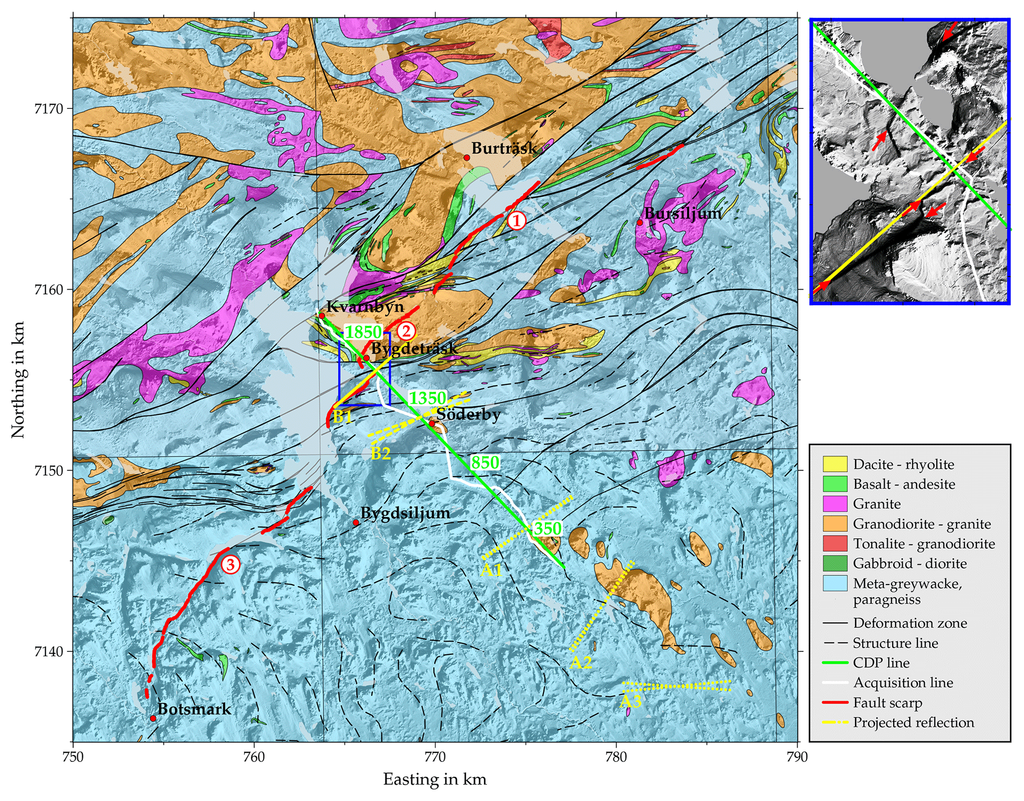
Figure 2Geological map of the survey area and location of the Burträsk profile. The Burträsk fault (red line) can roughly be divided into three parts, marked with the red numbers. The yellow lines mark the surface projection of reflector planes corresponding to the most prominent reflections in the seismic data with solid lines used for well-constrained surface locations and dotted lines for poorly constrained locations. Note that the actual reflection points are shifted laterally for reflectors with a large cross-dip component. The map inset shows an enlargement of the fault scarp and the red arrows indicate the location of the fault scarp. The location of the map is indicated in Fig. 1. Geological map © Geological Survey of Sweden; elevation data © Lantmäteriet.
Since 2007, a couple of reflection seismic profiles over post-glacial faults have been recorded. In the case of the Pärvie (Juhlin et al., 2010; Ahmadi et al., 2014) and Suasselkä faults (Kukkonen et al., 2009; Abdi et al., 2015), the fault scarps could be linked with dipping reflections, but for the Burträsk fault (Juhlin and Lund, 2011), no reflection directly connected to the fault scarp was observed. However, Juhlin and Lund (2011) imaged a dipping reflection which they could indirectly link to the fault. They attributed the lack of a clear reflection at the fault scarp to the crookedness of the profile and the complex geometry of the fault at the intersection with the seismic line (Fig. 2). The Burträsk fault is, however, of special interest since it is the seismically most active post-glacial fault and one of the most seismically active areas in all of Sweden. Therefore, we decided to reprocess the Burträsk dataset, applying an adapted cross-dip correction to the data.
This paper is divided into two parts. The objectives of the first part are to develop a local cross-dip correction module and to test its interactions with other processing steps to establish an optimized processing scheme. In the second part, we apply our cross-dip correction module to the Burträsk dataset to improve both the imaging of the fault and other reflectors below the profile and to refine the geological interpretation using information about the strike and dip of the reflections obtained by the cross-dip analysis.
The survey area is situated in the Paleoproterozoic rock formations of the southern Skellefteå district. The main structural feature of the area is a wide, dextral shear zone, suggested to have formed by lateral escape during the Svecokarelian orogeny (Romer and Nisca, 1995). Following Romer and Nisca (1995), we will refer to this feature as the Burträsk Shear Zone (BSZ). It was subdivided further by Rutland et al. (2001a), but for simplicity we continue using the original definition.
The BSZ marks the transition from metasedimentary rocks in the south to an area dominated by magmatic rocks in the north (Fig. 2). The metasedimentary rocks belong to the Bothnian supergroup – a sequence of sediments of mostly turbiditic origin that was accreted and metamorphosed during the Svecokarelian orogeny. They consist mainly of highly deformed and migmatized meta-greywackes, meta-argillites and paragneisses (Kathol and Weihed, 2005). The magmatic rocks in the northern part are attributed to two different phases of magmatism. The early Svecokarelian calc-alkaline intrusive rocks are mostly of granodioritic or tonalitic composition and are tentatively dated to 1.96–1.86 Ga (Kathol and Weihed, 2005). The late to post Svecokarelian granites likely originated from magmas derived from the middle and upper parts of the crust during a period of intense deformation and regional metamorphism at approximately 1.82–1.76 Ga (Kathol and Weihed, 2005). However, the exact tectonic evolution and timing of the magmatism in the area is still debated and a couple of different models exist (Rutland et al., 2001a; Rutland. et al., 2001b; Weihed, 2003; Juhlin et al., 2002; Lahtinen et al., 2009; Skyttä et al., 2012).
Similarly, the age of the BSZ is still discussed and suggestions range from 1.825 Ga (Romer and Nisca, 1995) to 1.86 Ga (Rutland et al., 2001a; Rutland. et al., 2001b; Skiöld and Rutland, 2006) and 1.895 Ga (Weihed et al., 2002). However, most authors agree that the peak of regional metamorphism in the area was around 1.825 Ga (Rutland et al., 2001a; Rutland. et al., 2001b; Weihed et al., 2002) and no major reactivation has so far been documented after 1.79 Ga. Since no borehole or seismic data are available, the geometry of the BSZ at depth is interpreted from surface observations and tectonic considerations. Romer and Nisca (1995) suggest a vertical strike-slip zone, whereas Rutland et al. (2001a) prefer an oblique fault with the hanging wall on the southern side.
The Burträsk fault scarp consists of a series of mostly southwest–northeast-oriented segments, together forming an approximately 35 km long lineament (Fig. 2). In the easternmost part, it follows a deformation line belonging to the BSZ (Fig. 2, “1”) and in the central part, it continues subparallel to the BSZ, cutting through a large intrusion east of Bygdeträsk (Fig. 2, “2”). In the westernmost part, the deformation zones of the BSZ change direction to a more east–west orientation and the fault scarp starts to diverge from the BSZ (Fig. 2, “3”). The fault scarp is usually 5–10 m high and generally covered by a variable layer of Quaternary sediments dominated by till, clay and silt. In a few locations, scarp outcrops forming slightly overhanging cliffs are observed (Lagerbäck and Sundh, 2008). Based on sediment liquefaction features close to Umeå, Mörner (2005) suggested a M>7 event for the formation of the fault scarp. On the other hand, Lagerbäck and Sundh (2008) found several sediment liquefaction and water escape structures during an extensive study of sediment deformation in the area but were not able to establish any relationship between the intensity of deformation and the proximity to the fault scarp.
3.1 Previous applications of the cross-dip correction
One of the main challenges of crooked acquisition lines is that the trace midpoints have an offset component perpendicular to the profile direction (Fig. 3). In the following, we will refer to this component as “cross-offset”. As a consequence, the depth to a reflector with a cross-dip component can vary for individual traces in a common depth point (CDP) gather, leading to an additional term in the travel time equation (Nedimović and West, 2003):
where t is the travel time; t0 is the zero time of the reflection; x is the inline offset; y is the cross-offset; h is the source-receiver distance; px is the slowness in profile direction and py the slowness perpendicular to the profile.
These time shifts are not accounted for in the standard normal moveout (NMO) processing which can result in focusing problems. Larner et al. (1979) defined the cross-dip correction Δtcross in the form of
where ϕ is the cross-dip angle and v is the medium velocity (Fig. 3).
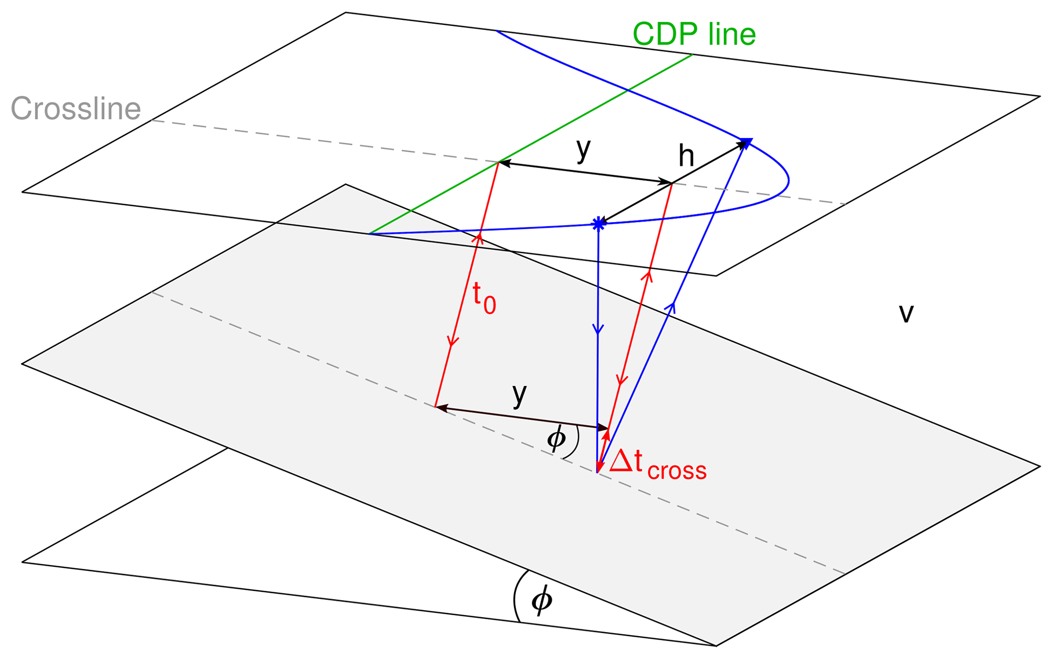
Figure 3Ray geometry for a crooked acquisition line above a cross-dipping reflector. y denotes the cross-offset, h the offset between shot and receiver, ϕ the cross-dip angle, v the medium velocity and t0 the zero-offset travel time for a ray without cross-offset.
The underlying assumption of this correction is that the reflector has no dip component in the profile direction (see Nedimović and West, 2003 for a more general form of the cross-dip correction).
The effect of uncorrected cross-dip on the stacked seismic section depends mainly on the distribution of the cross-offset, i.e., on the geometry of the acquisition line. Figure 4 shows a synthetic example of an NMO-corrected gather including two reflections affected by cross-dip at 0.4 s (A) and 1.2 s (B), respectively. The cross-offset distributions of these reflections correspond to the distributions at CDPs 350 and 1350 of the Burträsk profile (Fig. 2). The energy of the upper reflection (A) is completely smeared and is hardly visible in the stack (Fig. 4b). For the lower reflection (B), one cross-offset value is dominating the whole distribution, causing the energy to focus at 0.8 s instead of 1.2 s. As a result, the reflection appears in the stack but shifted in time (Fig. 4b).
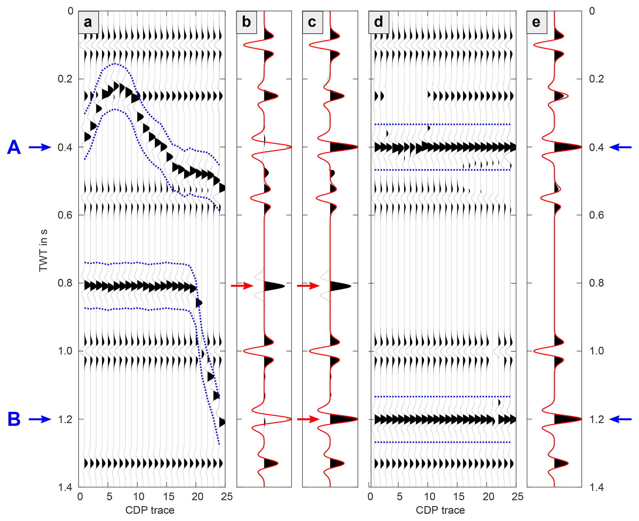
Figure 4Synthetic CDP gather illustrating the principle of the cross-dip correction. Panel (a) shows a NMO-corrected CDP gather including two reflections with 10∘ cross-dip originating at 0.4 s (A) and 1.2 s (B). The cross-offset distribution corresponds to the cross-offset distribution of CDPs 350 and 1350 of the Burträsk data and the dotted blue lines mark a window around the biased reflection time, t0+Δtcross. The comparison of the uncorrected stack (wiggle trace) with the theoretical stack (red line) in panel (b) indicates that reflection A is missing and reflection B is shifted. In the slant stack in panel (c), reflection A is correctly imaged but reflection B appears twice in the trace. The CDP gather after cross-dip correction in panel (d) shows that reflections A and B are shifted back to their origin time, t0. In the stack of the corrected CDP gather in panel (e), both reflections are correctly imaged.
Unlike the case for a reflector dipping in the profile direction, the cross-dip correction has no lateral component, but it requires specific knowledge of both cross-dip angle and velocity in the cross-profile direction or cross-slowness, respectively. Since these parameters are usually unknown, they have to be derived from the data.
Despite the simple form of Eq. (2), the correction has been applied in quite different ways by different authors. Initially, Larner et al. (1979) calculated the cross-dip correction simultaneously with the residual static solution. In their fundamental paper, Nedimović and West (2003) developed a procedure for an automated cross-dip correction where they invert for the cross-slowness by a grid search using the product of semblance and a local running average of the amplitudes as the objective function. For each estimated cross-slowness, they evaluate the reliability by thresholding the stack's amplitude and modal filtering. Finally, they correct for the estimated cross-dip while stacking using a slant stack approach. Other authors have used the same slant stack approach but with manually determined cross-dip values (Kim and Moon, 1992; Kim et al., 2014). A more simplistic approach is applying the cross-dip correction as a static shift to the whole trace (Wu et al., 1995; Rodriguez-Tablante et al., 2007; Lundberg and Juhlin, 2011; Ahmadi et al., 2014). However, this approach generally decreases the quality of all other reflections in the trace and is consequently mostly used for analyzing the cross-dips without applying the correction (Urosevic et al., 2007; Malehmir et al., 2009; Dehghannejad et al., 2010, 2012; Hedin, 2015).
While the problems with applying the cross-dip correction as a static shift are obvious, there are some more subtle disadvantages with implementing it using the slant stack approach. First of all, the slant stack procedure makes any further processing after the cross-dip correction impossible. This might be problematic since there are very likely interactions between cross-dip, DMO and NMO corrections. Another issue occurs when a CDP gather is dominated by one cross-offset value. In this case, the reflection occurs twice in the stack: at the origin time as well as at the shifted time corresponding to the dominating cross-offset (red arrows in Fig. 4c). To avoid this reflection duplication, we decided to use a method which moves the energy of a cross-dipping reflection to its origin time. Furthermore, we opted for a manual analysis of the cross-dip angles since automatic detection, as in the method of Nedimović and West (2003), is susceptible to noise and might pick up inline dip variations and NMO residuals resulting in unreasonably patchy dip distributions.
3.2 A new module for local cross-dip correction
We developed a module for a local cross-dip correction of individual reflections that can be directly used in a commercial software package. In our module, the reflections are approximated by a polygonal chain with the cross-dip values defined at the vertices of the chain. Between the vertices, the cross-dip values are linearly interpolated. For the actual correction, we use a cut-and-shift method where reflections affected by cross-dip are cut in a window around the biased reflection time t0+Δtcross (area between the dotted blue lines in Fig. 4a), shifted back by the correction term Δtcross and added to the trace at their origin time t0 (area between the dotted blue lines in Fig. 4d). This procedure leads to gaps in the corrected traces but is necessary to prevent reflection duplication as in the case of reflection B in Fig. 4c.
Along with the cross-dip values, the user defines the width of the correction window at each vertex and a constant velocity for the whole profile. We have decided to use the cross-dip angle as the main parameter since it is more intuitive than the cross-slowness, but it is very important to be aware of the coupling between cross-dip angles and velocities. Therefore, we recommend to translate variations and uncertainties in the velocity into a range of possible cross-dip angles for geological interpretation.
The module also includes an interactive function for analyzing the cross-dip angles. Analogous to velocity analysis, the cross-dip values can be picked interactively on stack panels corrected with a constant cross-dip angle. Thereby, it is possible to observe the effect of the correction on a whole reflection and not just on a CDP gather.
We created a series of synthetic test datasets using the same acquisition geometry as in the Burträsk dataset. The modeling is based on the simple modeling approach outlined by Ayarza et al. (2000). In this method, the travel times are calculated from the geometry of the acquisition line and the reflectors, while the amplitudes are obtained using the formulas of Aki and Richards (1980). The seismic traces are created by convolution of a scaled spike at the calculated travel time with a Ricker wavelet.
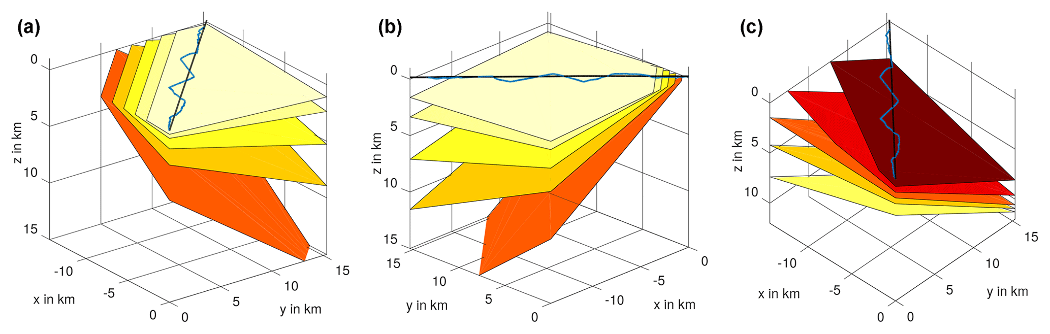
Figure 5Reflector geometry used in the synthetic modeling. Model 1 (a) comprises reflectors with 5, 10, 20, 30 and 45∘ cross-line dip from top to bottom. Model 2 (b) consists of a series of reflectors with 5, 10, 20, 30 and 45∘ inline dip. Model 3 (c) features reflectors with inline dips of 8.5, 16.1, 22.2, 26.6 and 29.1∘ and cross-line dips of 29.1, 26.6, 22.2, 16.1 and 8.5∘. The blue line represents the acquisition line and the black line the CDP line of the Burträsk dataset.
4.1 Model 1
The first model consists of a series of reflectors with increasing cross-dip in a constant velocity medium (Fig. 5a). The objectives of this model were to test the correction method and to analyze the effects of cross-dip on the stacked section. Figure 6a shows a stack of the synthetic data from model 1 using the true model velocities. Depending on the geometry of the acquisition line and the dip angle, the reflector cross-dip manifests itself as interference effects and smearing of the reflections in the stacked section. A subsequent analysis of the optimum stacking velocities yielded alternating high-/low-velocity patches mimicking the mean cross-offset. However, the stack quality remained poor for the reflections with larger cross-dips since the NMO correction can only account for hyperbolic travel time distortions (Fig. 6b). When applying our cross-dip correction module, we were able to retrieve the correct cross-dip angles for all reflectors and the reflections in the stacked section were effectively focused and flattened (Fig. 6c).
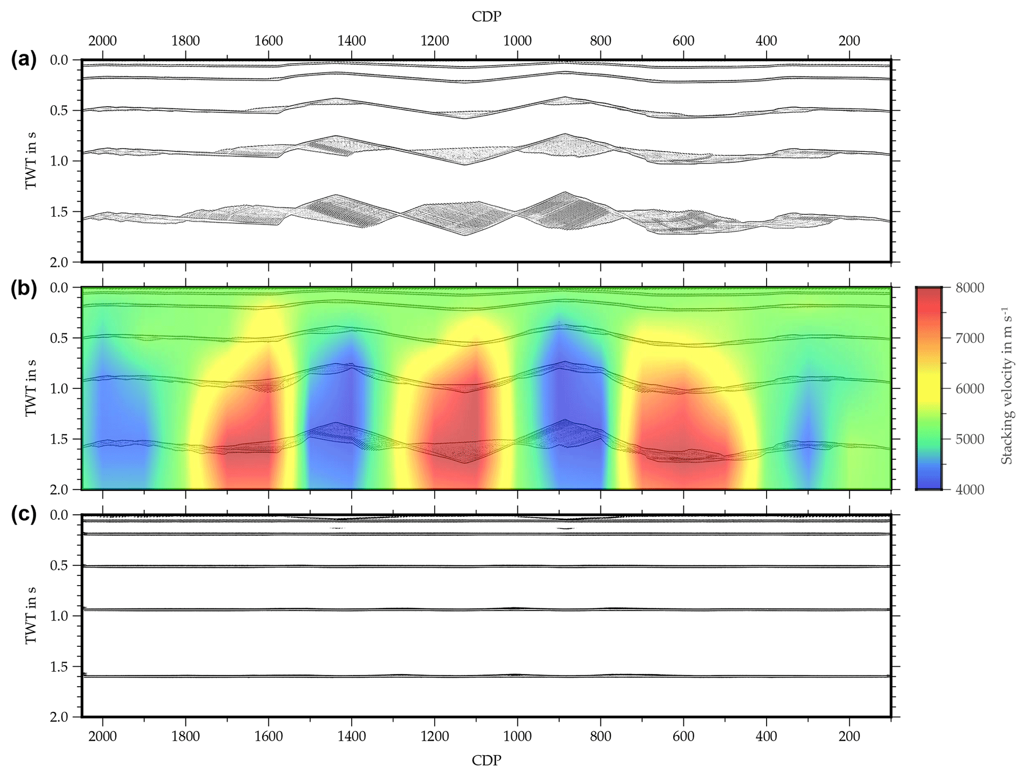
Figure 6Results of the first synthetic model with reflectors dipping in the cross-line direction. The reflections in the stacked section without cross-dip correction (a) are heavily deformed and smeared. Using the optimum stacking velocities instead of the model velocity (b) reduces the smearing locally, but the reflections remain distorted. After cross-dip correction, the reflections become focused and flattened (c).
4.2 Model 2
The second model was set up to evaluate how much inline dip can be picked up by the cross-dip correction and consisted of a series of plane reflectors with increasing inline dip in a constant velocity medium (Fig. 5b). As expected, it was not possible to find any cross-dip angles that consistently improved the stack of this dataset. Applying the cross-dip correction clearly distorts the reflections (Fig. 7). Some very localized focusing also occurs, but overall, the smearing of the reflections increases considerably.

Figure 7Results of the second synthetic model with reflectors dipping in the inline direction. Panel (a) shows a stack without cross-dip correction that exhibits the normal smearing due to inline dip. Panel (b) shows a stack with a constant cross-dip correction of −10∘ applied. The reflections get clearly distorted due to the falsely applied cross-dip correction. In most areas, smearing is increased but locally, reflections focus slightly.
4.3 Model 3
The aim of the third model was to test the interactions of the cross-dip correction and the DMO correction and to establish the preferred order of these steps in the processing flow. The model features a series of reflectors with different ratios of inline and cross-line dip in a constant velocity medium (Fig. 5c). Figure 8 shows two versions of the stacked section with (Fig. 8a) cross-dip correction applied before DMO correction and (Fig. 8b) after DMO correction. In the first case, picking the optimum cross-dip angle proved to be a bit challenging due to local maxima caused by the uncorrected inline dip. However, these occurred within a few degrees of the correct value and we were able to retrieve the expected values when picking with a focus on consistency. In the second case, similar difficulties arose because of artifacts introduced by the DMO correction. Again, focusing on consistency helped to identify the optimum cross-dip angles. In both versions of the stack, the reflections become flattened and focused, but the first version, with the cross-dip correction applied before the DMO correction, contains less artifacts and is slightly more coherent.
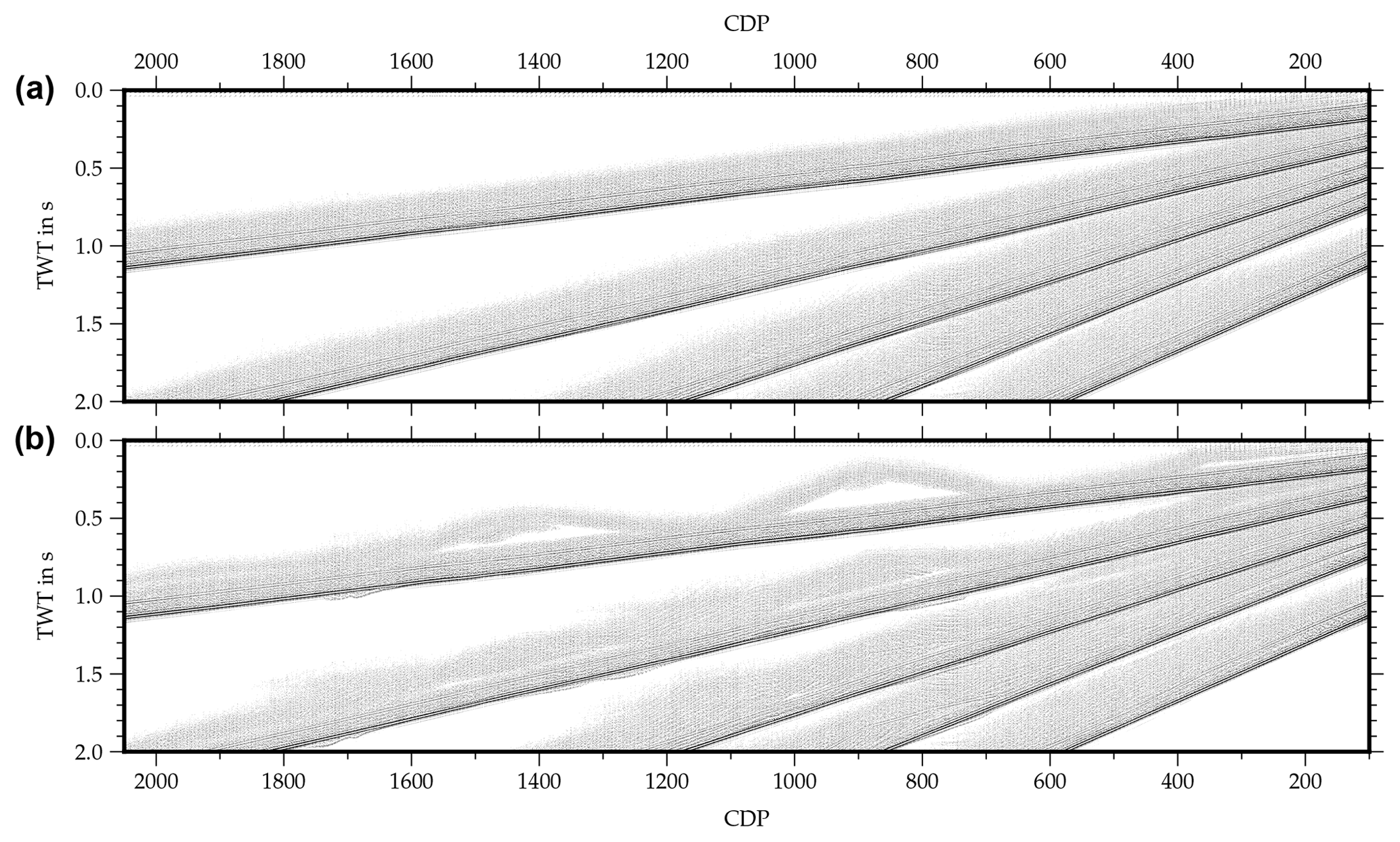
Figure 8Results of the third synthetic model with reflectors dipping in the inline and cross-line direction. Comparison of the stacked section with cross-dip correction before DMO correction (a) and with cross-dip correction applied after DMO correction (b). In both cases, the reflections become focused and flattened, but in the second case, artifacts are stronger.
4.4 Implications for the implementation of the cross-dip correction
As demonstrated clearly by the results of the first model, cross-dip effects can be picked up by stacking velocities, manifesting themselves as alternating high-/low-velocity patches. Therefore, it is important to reanalyze stacking velocities after correcting for cross-dip and to review the obtained cross-dip angles with the updated velocity model. Furthermore, the results from the second and third models highlight the importance of picking only cross-dip angles that consistently improve the image of a whole reflection (segment) in order to exclude local optima caused by interactions between the effects of inline and cross-line dip. The advantage of the manual cross-dip correction approach is that it is possible – to a certain extent – to identify and avoid these interactions, whereas the automatically conducted DMO correction is inevitably influenced by them.
Based on these results, we recommend an iterative processing scheme consisting of an initial sequence of NMO correction, cross-dip correction and velocity reanalysis followed by a second sequence of DMO correction and repeated velocity analysis. Both sequences should be repeated with the updated velocity models until no more significant improvements are achieved (Fig. 9). A surface-consistent residual static correction should be included at least once before the first iteration of the cross-dip correction sequence and can be repeated after each velocity analysis, if required. However, the interactions between residual statics and cross-dip correction are limited since the former is a surface-consistent shift of the whole trace, whereas the latter is a local shift of a small part of the trace depending on the mean cross-offset of each trace.

Figure 9Illustration of the iterative processing scheme for the implementation of the cross-dip and DMO corrections. The repetition of the residual static correction after each velocity reanalysis is optional.
These recommendations are only valid for a manual cross-dip correction. If the correction is derived automatically from the data, DMO should be applied first to avoid picking up local effects of inline dip.
5.1 Data processing
The approximately 22 km long Burträsk profile was acquired using an asymmetric split spread of 280 geophones with a natural frequency of 28 Hz. Both the receiver spacing and the nominal shot spacing were 20 m and the signal was generated using a VIBSIST hydraulic hammer source (Cosma and Enescu, 2001). Since the source could not be activated in the vicinity of buildings, shot coverage is quite sparse close to inhabited areas. As a result, the fold varies considerably over the profile (Fig. 10a). Similarly, the data quality is affected by random noise and coherent noise originating, e.g., from the source, surface waves and ground roll to a varying extent. All shot gathers have a relatively high background noise level, but some feature very distinct first arrivals and clearly visible reflections, whereas others show mostly noise with first arrivals barely identifiable after a few hundred meters (Fig. 11). As a first-order estimate of the average signal-to-noise ratio, Fig. 10a illustrates the ratio between the mean amplitude of the background noise in a 200 ms window before the first arrival and the mean amplitude of the first arrival in a 200 ms window starting at the first arrival (see also Fig. 11).
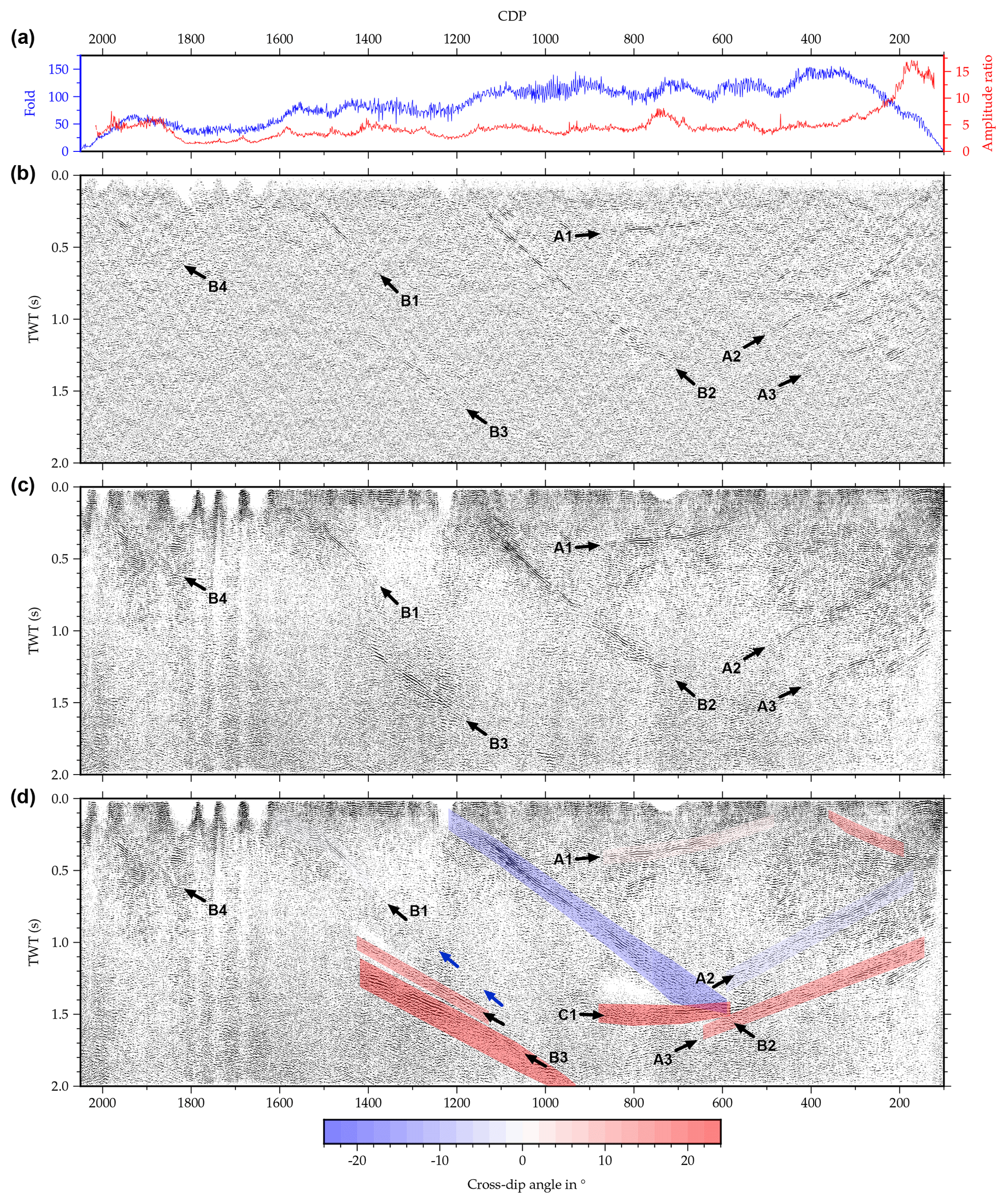
Figure 10Comparison between the original processing of the Burträsk dataset and the reprocessing at different stages: (a) fold distribution along the profile and mean amplitude ratio between the first 200 ms of data and the background noise; (b) original stack from Juhlin and Lund (2011); (c) reprocessed stack without cross-dip correction; (d) reprocessed stack with cross-dip correction overlain by the cross-dip angles used in the correction. The blue arrows indicate a possible continuation of reflection B1. The comparison of panels (b) and (c) highlights improvements due to the conventional reprocessing steps like statics, updated velocity model, etc., and the comparison of panels (c) and (d) illustrates the effects of the cross-dip correction.
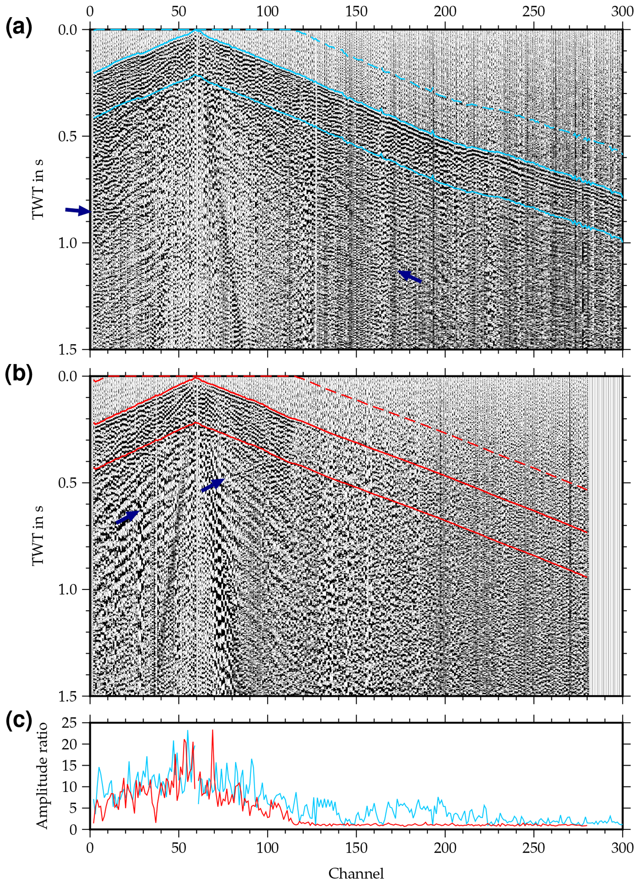
Figure 11Unprocessed shot gathers illustrating variations in the background noise level. The upper shot gather (a) displays very clear first arrivals along the whole spread, whereas the lower shot gather (b) is dominated by noise for larger offsets. The light blue and red lines mark the windows used for estimating the amplitude ratio between background noise and first arrival (c). The dark blue arrows indicate reflections.
The first part of the reprocessing followed the original processing flow from Juhlin and Lund (2011) quite closely. Due to the high noise level in some areas, we re-picked the first arrivals manually and reanalyzed the stacking velocities. We applied an additional ground-roll and first-break muting step following Oren and Nowack (2018). In their method, ground roll and first breaks are estimated by soft thresholding in the local time–frequency domain (Liu and Fomel, 2013) and subtracted from the data. Apart from that, there are only minor differences compared to the original processing, including slightly lower bandpass filter frequencies and a spherical divergence correction instead of an automatic gain control (AGC). A summary of the processing is given in Table 1.
Table 1Summary of the processing flow used for reprocessing the Burträsk dataset.
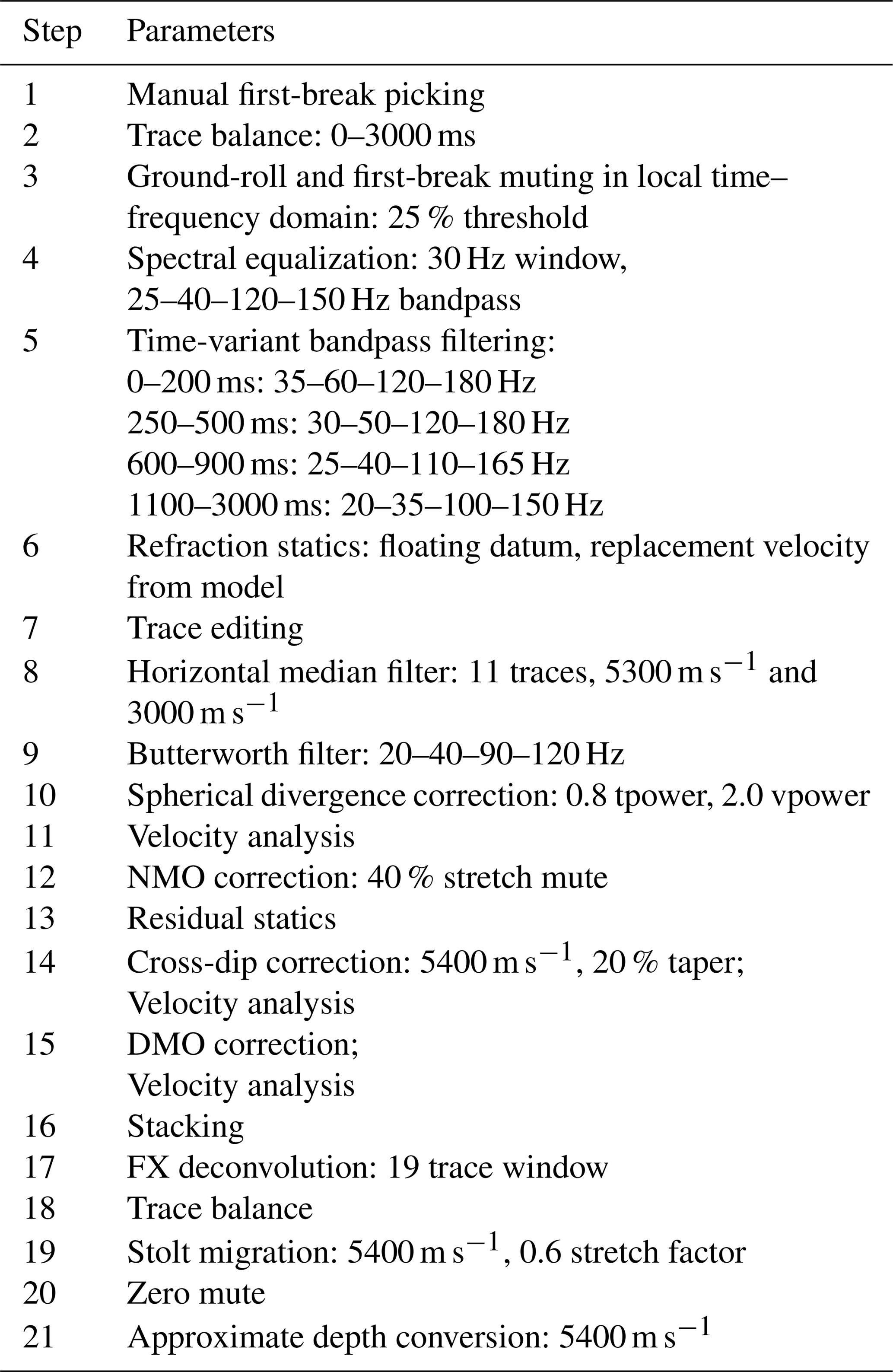
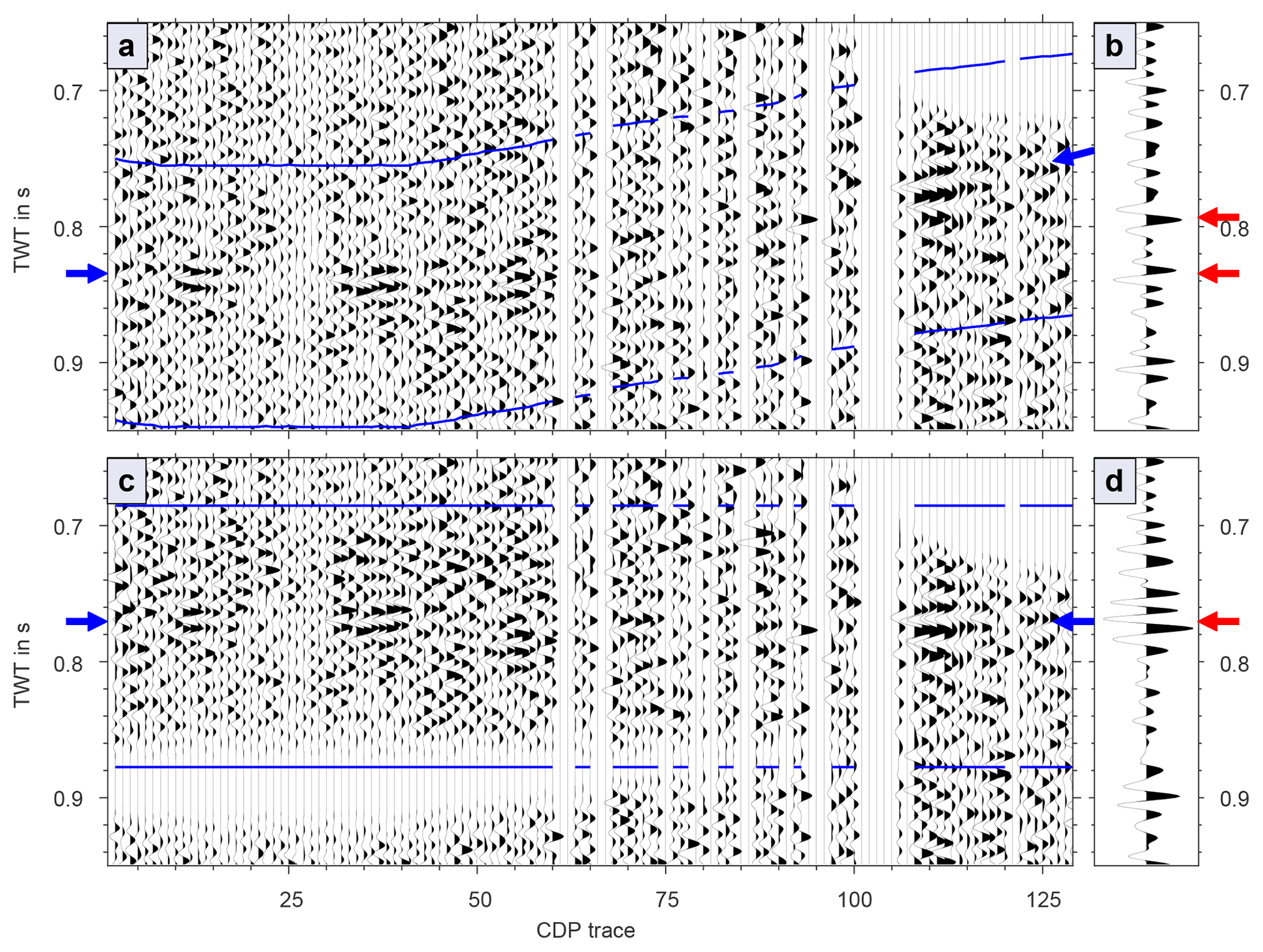
Figure 12Cross-dip correction of an NMO-corrected reflection in CDP 926 of the Burträsk data. In the uncorrected CDP gather (a), the reflection is approximately flat in the first traces and inclined in the later traces (correction window marked with blue lines). Consequently, the stack of this gather (b) features two weak maxima (red arrows). After cross-dip correction, the reflection gets flattened (c) and the weak maxima in the stack merge to one stronger maximum (d). Note, however, that the reflections are very difficult to observe in most other CDP gathers and that the cross-dip analysis has therefore been carried out on constant cross-dip stack panels.
Following the procedure outlined in the Sect. 4.4, we incorporated the cross-dip correction directly after the residual static correction and reanalyzed the velocities. With the new velocity model, we updated the cross-dip angles and repeated the velocity analysis. Following this, we iteratively applied DMO correction and velocity reanalysis. Repeating the residual static correction did not lead to any significant improvements. Figure 12 illustrates the effect of the cross-dip correction in CDP gather 926. However, this CDP is not representative, as most gathers feature much higher noise levels, making it very difficult to observe the focusing of reflections. Therefore, the cross-dip analysis was carried out on constant cross-dip stack panels. During the first pass of the cross-dip and DMO correction sequences, the velocities changed substantially after each step but converged during the second pass. The final stacking velocity model is much more consistent along individual reflections than the initial one but seems to be still biased by dip effects. For comparison, we also tested another processing scheme, where the cross-dip correction is applied after the DMO correction, but could not produce a stack of comparable clarity.
Migration testing using a smoothed stacking velocity model for migration yielded poor results, confirming that the stacking velocities are still biased by residual dip effects. Among tests with Kirchhoff migration, finite difference migration, different phase-shift migration algorithms and Stolt migration, the best results were archived for a Stolt migration with a constant velocity of 5400 m s−1. This velocity is also consistent with the velocities obtained during the refraction static correction. Finally, the section was depth converted using the same constant velocity. However, it is important to note that the depth values are only an estimation of the real depth since considerable uncertainties exist in the deeper part, where the velocity is poorly constrained.
Additional to the reflection seismic processing, we carried out first-break tomography using the PStomo_eq solver by Tryggvason et al. (2002, 2009). To simulate a thin velocity layer above the bedrock, we used a 2-D starting model with a steep velocity increase from 1500 to 5400 m s−1 in the first 40 m below the surface and a gradual velocity increase to 5800 m s−1 towards the bottom of the model. We conducted the inversion on a 3-D grid with a cell size of while simultaneously estimating a static solution to eliminate the influence of subgrid-scale velocity variations on the model. To estimate the resolving power of the tomographic model, we ran a checkerboard test using the starting model perturbed with a 3-D pattern of 500 m wide and 100 m thick checkers (Fig. S1 in the Supplement). For the inversion of the checkerboard model, we used the same parameters as in the main inversion but did not estimate a static solution. The results show that the uppermost checkers, including the bedrock surface, are reconstructed well but most of the lower checkers are poorly reconstructed or not reconstructed at all, indicating that only velocity variations close to the bedrock surface can be resolved properly and that the lower part of the tomographic model is poorly constrained.
5.2 Results
Figure 10 shows a comparison between the unmigrated original stack (Fig. 10b), a reprocessed version of the stack excluding the cross-dip correction (Fig. 10c) and a reprocessed version including the cross-dip correction (Fig. 10d). The comparison of Fig. 10b and c, both conventional DMO stacks, illustrates the effects of the basic reprocessing of the data (mainly an improved refraction and residual static correction, an improved velocity model and first-break and ground-roll muting). The comparison of Fig. 10c and d isolates the changes caused by the cross-dip correction. The original stack contains a series of northwest-dipping reflections and reflection packages, referred to as A1–A4, and a series of southeast-dipping reflections, named B1–B3. Even without the cross-dip correction, the reprocessing enhanced the continuity and coherency of the reflections considerably. Especially reflections A3, B3 and B4, which are barely visible in the original stack, are imaged much clearer after the basic reprocessing.
Table 2Estimated strike and dip of the most prominent reflections.
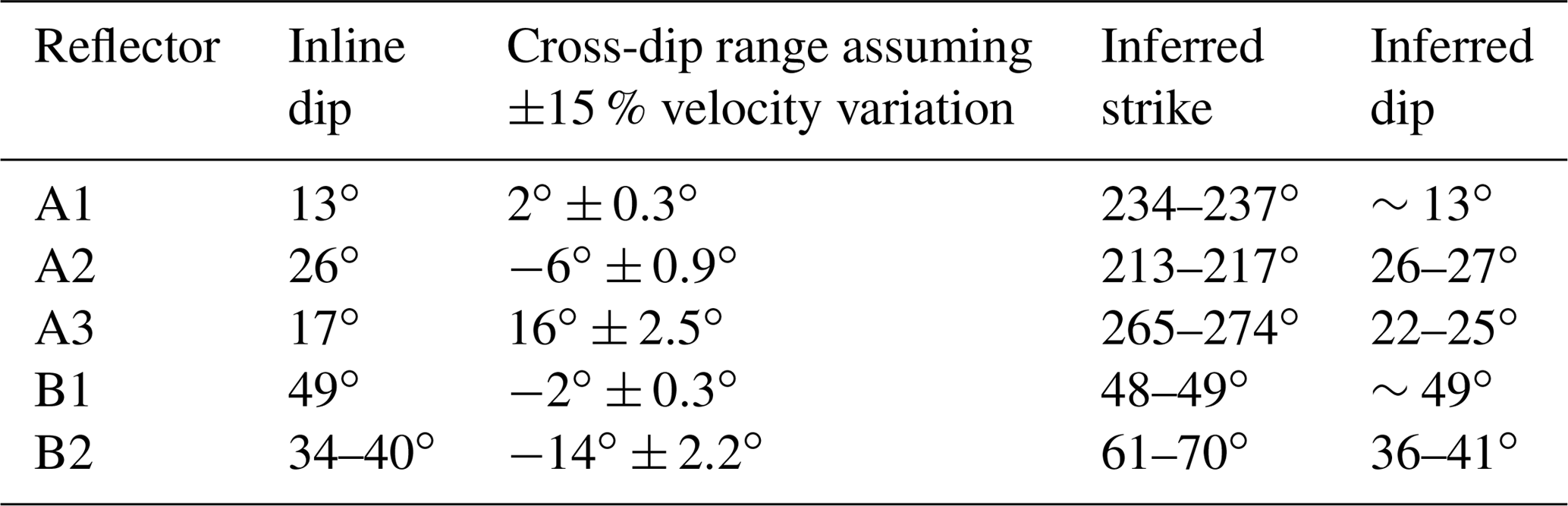
Reflection B2 branches in the upper part; therefore, we used two different inline dip values in the estimation.
Analysis of the cross-dip angles yielded mostly values in the range of ±16∘, except for two deeper reflection packages, both with a cross-dip of 24∘ (Fig. 10d). Northwest of CDP 1600, cross-offsets proved to be too small to determine any cross-dip angles. The effect of the cross-dip correction on the individual reflections depends to a large extent on their respective cross-offset distribution and cross-dip angle. Not surprisingly, there is little change for the mainly inline-oriented A1 and B1 reflections (Fig. 10). Reflections A2 and A3, which are in an area with comparably small cross-offsets, become more focused and can be followed to greater depth after cross-dip correction but stay essentially in the same position. In contrast to this, reflections B2 and B3 have vertical shifts of up to 100 ms caused by large, unevenly distributed cross-offsets. As a result of these shifts, reflection B2 loses its slightly listric appearance (Fig. 10). Moreover, two reflections appear only after cross-dip correction: a rather weak reflection directly above reflection package B3 and a subhorizontal reflection package close to the lower end of reflection B2, called C1 in the following (Fig. 10d).
Before converting inline and cross-dip angles into strike and dip of the reflection, the possible range of velocities should be translated into a possible range of cross-dip values. Table 2 shows inferred strike and dip values for a ±15 % velocity variation, corresponding to a velocity range of 4590 to 6210 m s−1. Note that this is not an error estimate since it does not include uncertainties in the picking of the cross-dip values.
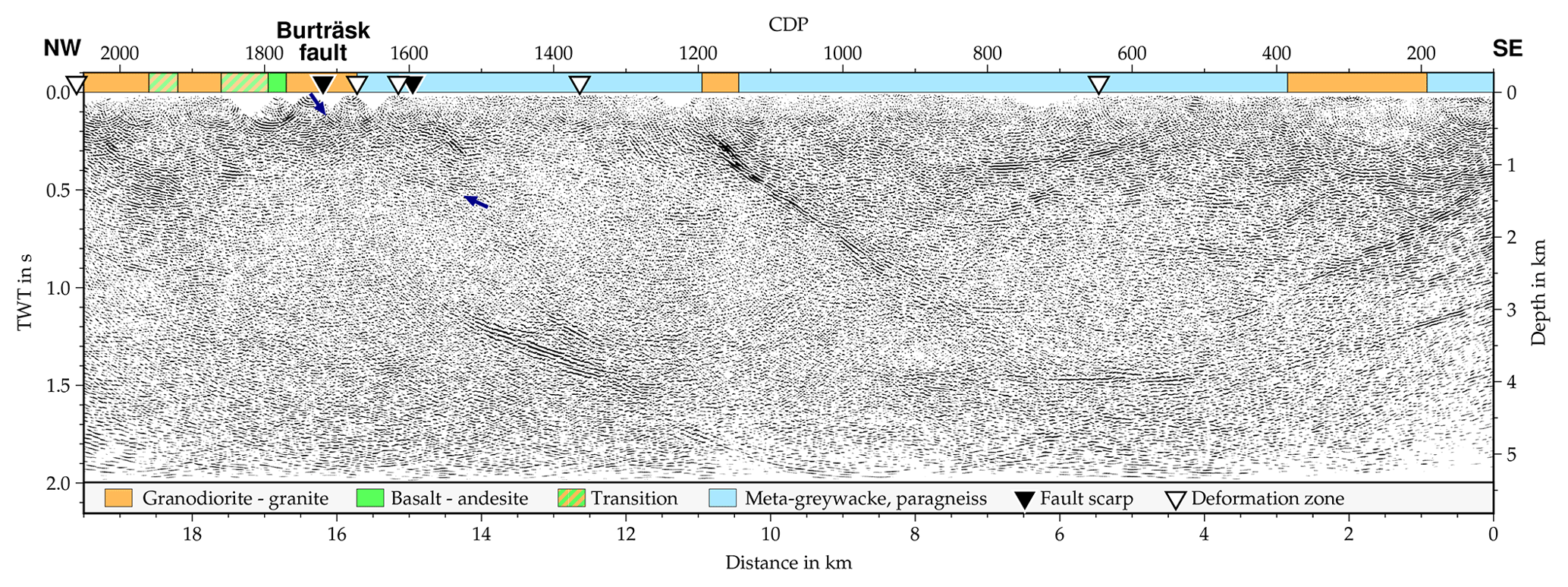
Figure 13Migrated section along the Buträsk profile. For comparison, the surface geology is plotted on top of the section and the location of the fault scarp and deformation zones are marked. The small blue arrows highlight a very weak reflection that might be associated with the fault scarp. The vertical exaggeration of the section is approximately 1.
None of the abovementioned reflections are associated with the segment of the fault scarp intersecting the seismic line at CDP 1720. There are some indications of dipping reflections which might be connected to the fault scarp, but these are too weak to interpret with confidence (Fig. 13). However, the surface projection of reflection B1 coincides with the extrapolation of the scarp segment west of the seismic line around CDP 1600 (Fig. 2). At the same location, the geological map features a deformation zone, but the strike does not agree well with the estimated strike of reflection B1 (Fig. 2).
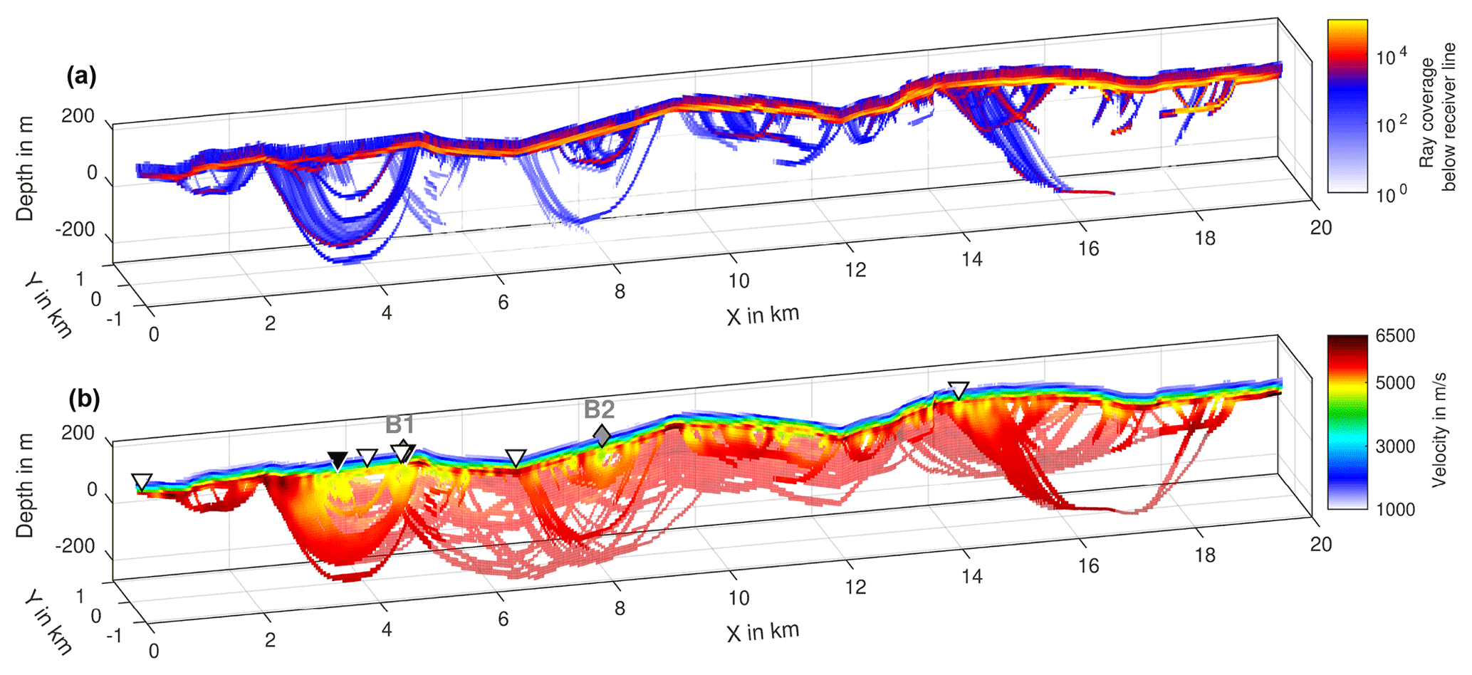
Figure 14A 2-D slice of the ray coverage and the velocity model from the first-break tomography. Panel (a) shows the ray coverage in a 100 m wide zone below the receiver line. Panel (b) displays the velocity below the receiver line in bright colors. In areas without velocity information below the receiver line, the average of the velocity model in the y direction is plotted in dim colors. The black triangles mark the location of the fault scarp, the white triangles indicate deformation zones and the grey diamonds correspond to the surface projection of reflections B1 and B2. The vertical exaggeration of the model section is 5.
Figure 14 shows the velocity model from the first-break tomography. Due to the sparse spatial coverage, we reduced the 3-D model to a 2-D image displaying the mean of the model within 100 m distance from the receiver line in bright colors and otherwise the average of the model in the cross-line direction in pale colors. Due to the high velocity contrast between the Quaternary sediments and the bedrock, most rays were guided along the bedrock surface and did not penetrate into the deeper parts.
In the upper part of the bedrock, the velocity is mainly around 5300–5500 m s−1 and increases slightly with depth (Fig. 14) but this might be an artifact of the starting model since the checkerboard test indicated that the velocity is not well resolved in the lower parts of the model. The model features several low-velocity zones, the largest one at around x=4.0 km to x=4.5 km and coinciding with the location of the fault scarp, some smaller ones around x=5.0 km, x=5.5 km and x=9.0 km and a couple of very localized ones throughout the whole profile.
6.1 Cross-dip correction
Both synthetic modeling and the field data example have clearly demonstrated the benefits of applying the cross-dip correction to crooked-line seismic data. As several previous studies have already illustrated, cross-dip can de-focus and smear reflections, resulting in a poor stacked image (e.g., Larner et al., 1979; Kim and Moon, 1992; Nedimović and West, 2003). Another quite rarely mentioned aspect is that it can lead to vertical shifts, distortion and duplication of out-of-plane reflections as well. Our local cross-dip correction addresses this problem by shifting back reflections affected by cross-dip and thereby projecting them into the CDP plane. However, the drawback of this procedure is that it cannot handle crossing reflections very well. Therefore, the applicability of our method to areas with complex, distributed reflectivity patterns is limited. In such areas, more extensive testing is needed to develop an appropriate correction scheme since existing schemes, like the one of Nedimović and West (2003), do not account for the reflection duplication problem.
Apart from improving the imaging of crooked-line seismic data, the cross-dip correction has the advantage of extracting information on the 3-D orientation of reflections, information which can be crucial for the geological interpretation of the seismic data. This can be especially important in low signal-to-noise data with low fold where sparse swath 3-D processing is not an option.
6.2 Data reprocessing
Processing crooked-line seismic data from hardrock settings includes a whole range of different challenges. Apart from cross-dip effects, imaging quality is often affected by residual static shifts, surface waves, coherent noise, strong ground roll, etc. As in many other studies (e.g., Juhlin, 1995; Pretorius et al., 2003; Urosevic et al., 2007; Place and Malehmir, 2016), the most important steps in the basic reprocessing of the data proved to be the manual picking of first arrivals for improving the static correction and a careful velocity analysis. Furthermore, the comparison between Fig. 10b and c illustrates that the final image benefited considerably from using an analytical gain instead of applying an AGC since the contrast between the main reflections and the background reflectivity is preserved.
6.3 Origin of the reflections
The reflections in the final stack are mostly planar and occur in a relatively low reflectivity surrounding (Fig. 13). There are different possible origins for such reflections. The first possibility is a contact between different lithological units. Along the CDP line, the surface geology map features several lithological contacts (Figs. 2 and 13), but these contacts will only produce reflections if there is a significant difference in seismic impedance between the two lithological units. Both the output bedrock velocity from the refraction static correction and the first-break travel time tomography do not show any significant changes in bedrock velocity along the profile. This observation, along with the lack of correlation between the seismic reflections and surface geology (Fig. 13) and the fact that some reflections are clearly cross-cutting subhorizontal background reflections (Fig. 13), makes lithological contacts a rather unlikely candidate. A second possibility is deformation or shear zones with either decreased or increased seismic impedance due to fracturing and/or remineralization processes. Whether or not such zones are visible in seismic data depends not only on the impedance contrasts but also on the width of the zones. Theoretically, features with a minimum width of (Sheriff and Geldart, 1995), corresponding to 2.4–4.5 m for a peak frequency of 60–75 Hz and a velocity of 5400 m s−1 in this survey, are detectable in seismic reflection images. In practice, the detectability limit depends strongly on the signal-to-noise ratio of the data. In the Burträsk survey, the signal level is relatively low, so a more realistic estimation of the detectability limit is , corresponding to a width of 6–11.25 m. Since the profile intersects a couple of deformation zones belonging to the BSZ (Fig. 2), it is quite plausible that some of the reflections are caused by shear zones. Another possible scenario is that some reflections originate from magmatic dykes and/or sills. The Burträsk area was subject to intense migmatization and hosts intrusions from different magmatic pulses prior to, during and after the Svecokarelian orogeny (Kathol and Weihed, 2005). Thus, both sills and dykes are likely to occur along the profile. Due to the quite non-impulsive nature of the signal (even after deconvolution) and the high noise level, it is not possible to infer any reliable information about the internal structure of the reflections from an analysis of polarity and tuning effects.
In the following, we will discuss the nature of the most important reflections in the Burträsk profile. B1 is a relatively weak planar reflection that can only be observed clearly over a short depth interval, but in the unmigrated stack there are some indications that it might continue to greater depths (Fig. 10). Moreover, it seems to cut through the mostly subhorizontal background reflectivity (Fig. 13), arguing against a lithological boundary. Since the surface projection of reflection B1 coincides both with a projection of the western scarp segment (Fig. 2) and a low-velocity zone in the tomography model (Fig. 14), we interpret B1 as a reflection from either the western scarp segment itself or from the continuation of the shear zone along which the western scarp segment has ruptured. The small vertical extent of the reflection might be explained by a rather narrow shear zone that drops below the detection limit as the frequency content and signal strength decrease with depth.
Similar to B1, reflection B2 cross cuts subhorizontal background reflections (Fig. 13) and its surface projection coincides with a narrow low-velocity zone in the tomography model (Fig. 14). Again, we interpret B2 as a reflection from a shear zone, but the relation to the Burträsk fault is less obvious. The prominence of the reflection might suggest that the movement of the post-glacial fault at depth took place along reflection B2 and that the visible fault scarp segments are merely the branches of that fault where the surface rupture occurred. Branching of post-glacial fault scarps seems to be a common phenomenon and has been observed for the Pärvie and Lansjärv faults (Talbot, 1986; Juhlin et al., 2010; Ahmadi et al., 2015). Since the Burträsk fault is seismologically very active, earthquake locations might give a hint which fault plane is active at depth. Recent studies show the micro-earthquakes clustering along a southeast-dipping plane, but unfortunately, the accuracy of the locations is not sufficient to distinguish between the closely spaced B1 and B2 reflections (Lund et al., 2016). In any case, B2's estimated strike of 61–70∘ is not consistent with the strike of the fault scarp but rather matching the trend of the BSZ in the southern part (Fig. 2). Therefore, we prefer to interpret B2 as a reflection from a local shear zone belonging to the BSZ and not connected to the Burträsk fault. It is, however, still possible that B2 extends further to the southwest and connects with the westernmost scarp segment.
Since reflection B4 projects to the surface close to a mapped deformation zone (Fig. 2), we tentatively interpret it as another local shear zone belonging to the BSZ.
Both of the two deepest reflections, B3 and C1, exhibit strong reflectivity and terminate very abruptly at the upper end. Neither data fold and amplitude ratio (Fig. 10a) nor the overall impression of the image quality (Figs. 10d and 13) indicate a significant drop in data quality, so the abrupt terminations seem to be real features. Together with the high reflectivity, this suggests that reflections B3 and C1 are caused by sill or dike intrusions (Planke et al., 2005).
Unlike most of the other reflections, A2 and A3 are dipping to the northwest and their approximate surface projections are well south of the BSZ (Fig. 2). At 0.8 s, reflection A2 is clearly intersecting with a subhorizontal reflection segment (Figs. 10d and 13), precluding the possibility of a lithological contact. The geometry of reflections B2, A2 and A3 and the apparently lower dip of reflection A3 could be interpreted as a positive flower structure, consistent with the proposed oblique convergence of the Skellefteå district from the southeast (Bergman-Weihed, 2001). However, the true dips of reflections A2 and A3 are relatively small and very similar (Table 2) and the estimated strikes of reflections A2, A3 and B2 do not match at all (Fig. 2). So in this case, the additional information from the cross-dip analysis argues against the hypothesis of a flower structure. Instead, the occurrence of several magmatic bodies southeast of the profile points towards a magmatic origin of the reflections, possibly as feeder dikes following pre-existing weak zones in the upper crust. It is not clear from the present dataset how reflection A1 should be interpreted.
Even though only reflections B1 and B4 can be directly correlated with deformation zones in the geological map, the dominance of southeast-dipping reflections in the northwestern part of the profile suggests that the BSZ formed as a an oblique fault system, as interpreted by Rutland et al. (2001a), and not as a vertical strike-slip zone, as suggested by Romer and Nisca (1995).
6.4 Imaging of the fault scarp
The lack of a clear reflection connected to the fault scarp at CDP 1710 might be due to several different reasons. First of all, it could be caused by the absence of a resolvable contrast in physical properties. As discussed above, the fault zone needs to have a certain minimum width to be detectable in the seismic data. However, the post-glacial Pärvie and Suasselkä faults have successfully been imaged with reflection seismic data using very similar acquisition parameters (Juhlin et al., 2010; Abdi et al., 2015, respectively). So if the Burträsk fault has similar characteristics, it should be well detectable in the seismic data. Another possibility is that the reflections from the fault scarp are not stacked properly due to the complex, three-dimensional geometry of the fault at the profile location. In this case, the reflections should still be clearly visible in the shot gathers. The shot gathers, however, exhibit only very blurred dipping reflections covered by various forms of noise. Figure 10a shows that, between CDPs 1600 and 1800, both the data fold and the average amplitude ratio between first arrival and the background noise are exceptionally low, indicating a poor signal-to-noise ratio. Therefore, the most likely explanation for the lack of a reflection connected to the fault scarp is simply the result of insufficient data coverage and quality.
6.5 Relation between post-glacial fault and BSZ
The relation between the Burträsk fault and the BSZ is still not fully understood. Compared to the majority of the known post-glacial faults, which predominantly strike north–northeast, the Burträsk fault has an unusually strong east–west component. In contrast to this, the neighboring Röjnoret fault is mostly north–south oriented, following yet another set of Paleoproterozoic shear zones (Fig. 1). This divergence from the main trend of post-glacial faults might indicate that the faults in the Skellefteå area were to a very large extent guided by pre-existing weak zones in the crust. However, the Burträsk fault only follows individual deformation zones closely in the northernmost part (Fig. 2, “1”) and runs subparallel to the BSZ in the central part (Fig. 2, “2”). Since the reflection seismic image has shown that there are potentially many more shear zones than the ones marked in the geological map, it is likely that the fault still follows weakness zones belonging to the BSZ. South of the large jump north of Bygdsiljum, the fault scarp starts to diverge significantly from the BSZ where the latter turns to a more east–west orientation (Fig. 2, “3”), suggesting that the orientation of the BSZ was no longer conducive to the prevailing stress field controlling the rupture direction. Therefore, we speculate that the BSZ acted as a guide for the Burträsk fault, causing its orientation to deviate from the orientation of the majority of post-glacial faults. During the rupture, the fault probably jumped between different weak zones to accommodate differences between the orientation of the BSZ and the orientation of the minimum horizontal stress.
In the first part of this paper, we presented a new software module for a local cross-dip correction and tested the influence of cross-dip on synthetic seismic data. An often forgotten effect of cross-dip is that – depending on the cross-offset distribution – it cannot only de-focus and smear reflections but also shift them in time. Most existing cross-dip routines rely on a slant stack approach for the correction which has the drawback that shifted reflections will appear twice in the stack. Within our new module, we use a shift and stack method to overcome this reflection duplicating problem and enable further processing after the correction. The synthetic test examples demonstrate that the cross-dip correction can interact both with the stacking velocities and the DMO correction. Based on these tests, we proposed an iterative processing scheme where a sequence of cross-dip correction, velocity analysis, DMO correction and velocity analysis is repeated until the stacked image converges.
In the second part of this paper, we presented results of reprocessing data from the Burträsk profile using our new module. After cross-dip correction, several reflections became significantly more continuous and coherent. An improved static solution and the use of an analytical gain also contributed considerably to the quality of the final image. The improvements we achieved during reprocessing illustrate the often underestimated potential of relatively simple methods, like the cross-dip correction and the traditional filtering and muting, in processing noisy hardrock seismic datasets. Moreover, strike and dip values estimated from the cross-dip angles helped in associating the seismic reflections with geological features. We interpreted most of the southeast-dipping reflections as shear zones belonging to the BSZ, implying that the BSZ is not a vertical but a southeast-dipping feature. The north- to northwest-dipping reflections in the southernmost part of the profile are likely attributed to magmatic intrusions. Due to the low data fold and high noise level close to the Burträsk fault, the scarp segment intersecting with the profile could not be imaged. However, we obtained a clear reflection from another scarp segment slightly further west, dipping southeast at approximately 49∘.
The underlying research data are available via the Swedish National Data Service. The following data files are available for download: the raw shot gathers with geometry information in the headers (Juhlin and Lund, 2019a); the original stacked section from Juhlin and Lund (2011; Juhlin and Lund, 2019b); the cross-dip-corrected stacked section (Juhlin and Beckel, 2019a); the depth-converted, cross-dip-corrected migrated section (Juhlin and Beckel, 2019b).
The supplement related to this article is available online at: https://doi.org/10.5194/se-10-581-2019-supplement.
CJ and RAB conceived the analysis method. RAB developed the software module (written for GLOBE Claritas™, available via personal communication) and carried out the data analysis and interpretation. RAB prepared the manuscript and CJ reviewed it.
The authors declare that they have no conflict of interest.
This article is part of the special issue “Advances in seismic imaging across the scales”. It is a result of the 14th International Symposium on Deep Seismic Profiling of the Continents and their Margins, Kraków, Poland, 17–22 June 2018.
GLOBE Claritas™ under license from the Institute of Geological and Nuclear Sciences Limited, Lower Hutt, New Zealand, was used to process the seismic data. The Generic Mapping Tools (GMT) package was used to prepare many of the figures.
This paper was edited by Ramon Carbonell and reviewed by two anonymous referees.
Abdi, A., Heinonen, S., Juhlin, C., and Karinen, T.: Constraints on the geometry of the Suasselkä post-glacial fault, northern Finland, based on reflection seismic imaging, Tectonophysics, 649, 130–138, 2015. a, b
Ahmadi, O., Juhlin, C., and Gessner, K.: New Insights from Seismic Imaging over the Youanmi Terrane, Yilgarn Craton, Western Australia, Energy Proced., 59, 113–119, 2014. a, b
Ahmadi, O., Juhlin, C., Ask, M., and Lund, B.: Revealing the deeper structure of the end-glacial Pärvie fault system in northern Sweden by seismic reflection profiling, Solid Earth, 6, 621–632, https://doi.org/10.5194/se-6-621-2015, 2015. a
Aki, K. and Richards, P. G.: Quantitative Seismology I, Wh Freeman & Co, San Francisco, USA, 1980. a
Arvidsson, R.: Fennoscandian Earthquakes: Whole Crustal Rupturing Related to Postglacial Rebound, Science, 274, 744–746, 1996. a
Ayarza, P., Juhlin, C., Brown, D., Beckholmen, M., Kimbell, G., Pechnig, R., Pevzner, L., Ayala, C., Bliznetsov, M., Glushkov, A., and Rybalka, A.: Integrated geological and geophysical studies in the SG4 borehole area, Tagil Volcanic Arc, Middle Urals: Location of seismic reflectors and source of the reflectivity, J. Geophys. Res., 105, 21333–21352, 2000. a
Bergman-Weihed, J.: Economic geology research, chap. Palaeoproterozoic deformation zones in the Skellefte and Arvidsjaur areas, northern Sweden, Geological Survey of Sweden, Uppsala, Sweden, 46–69, 2001. a
Bödvarsson, R., Roberts, R., Lund, B., and Slunga, R.: Earthquake activity in Sweden, Report R-06-67, Swedish Nuclear Fuel and Waste Management Co, Stockholm, Sweden, 2006. a
Cosma, C. and Enescu, N.: Characterization of fractured rock in the vicinity of tunnels by the swept impact seismic technique, Int. J. Rock Mech. Min., 38, 815–821, 2001. a
Dehghannejad, M., Juhlin, C., Malehmir, A., Skyttä, P., and Weihed, P.: Reflection seismic imaging of the upper crust in the Kristineberg mining area, northern Sweden, J. Appl. Geophys., 71, 125–136, 2010. a
Dehghannejad, M., Bauer, T. E., Malehmir, A., Juhlin, C., and Weihed, P.: Crustal geometry of the central Skellefte district, northern Sweden – constraints from reflection seismic investigations, Tectonophysics, 524–525, 87–99, 2012. a
Du Bois, L., Levato, L., Besnard, J., Escher, A., Marchant, R., Oliver, R., Ouwehand, M., Sellami, S., Steck, A., and Wagner, J. J.: Pseudo-3D study using crooked line processing from the Swiss Alpine western profile – Line 2 (Val d'Anniviers-Valais), Tectonophysics, 173, 31–42, 1990. a
Hedin, P.: Geophysical studies of the upper crust of the central Swedish Caledonides in relation to the COSC scientific drilling project, PhD thesis, Uppsala University, Uppsala, Sweden, 2015. a
Juhlin, C.: Imaging of fracture zones in the Finnsjön area, central Sweden, using the seismic reflection method, Geophysics, 60, 66–75, 1995. a
Juhlin, C. and Beckel, R.: Reflection seismic study of the post-glacial Burträsk fault: Cross-dip stack. Swedish National Data Service. Version 1.0. Uppsala University, Department of Earth Sciences, https://doi.org/10.5878/qwm7-pz92, 2019a. a
Juhlin, C. and Beckel, R.: Reflection seismic study of the post-glacial Burträsk fault: Migrated cross-dip stack. Swedish National Data Service. Version 1.0. Uppsala University, Department of Earth Sciences, https://doi.org/10.5878/k3zc-s495, 2019b. a
Juhlin, C. and Lund, B.: Reflection seismic studies over the end-glacial Burträsk fault, Skellefteå, Sweden, Solid Earth, 2, 9–16, https://doi.org/10.5194/se-2-9-2011, 2011. a, b, c, d, e
Juhlin, C. and Lund, B.: Reflection seismic study of the post-glacial Burträsk fault: Shot gathers with geometry. Swedish National Data Service. Version 1.0. Uppsala University, Department of Earth Sciences, https://doi.org/10.5878/g1mw-0h64, 2019a. a
Juhlin, C. and Lund, B.: Reflection seismic study of the post-glacial Burträsk fault: Original stack. Swedish National Data Service. Version 1.0. Uppsala University, Department of Earth Sciences, https://doi.org/10.5878/gs5z-p737, 2019b. a
Juhlin, C., Elming, S.-Å., Mellqvist, C., Öhlander, B., Weihed, P., and Wikström, A.: Crustal reflectivity near the Archaean-Proterozoic boundary in northern Sweden and implications for the tectonic evolution of the area, Geophys. J. Int., 150, 180–197, 2002. a
Juhlin, C., Dehghannejad, M., Lund, B., Malehmir, A., and Pratt, G.: Reflection seismic imaging of the end-glacial Pärvie Fault system, northern Sweden, J. Appl. Geophys., 70, 307–316, 2010. a, b, c
Kathol, B. and Weihed, P. (Eds.): Description of regional geological and geophysical maps of the Skellefte District and surrounding areas, Geological Survey of Sweden, Report Ba 57, Uppsala, Sweden, 2005. a, b, c, d
Kim, J. and Moon, W. M.: Seismic imaging of shallow reflectors in the eastern Kapuskasing structural zone, with correction of crossdip attitudes, Geophys. Res. Lett., 19, 2035–2038, 1992. a, b, c
Kim, J. S., Lee, S. J., Seo, Y. S., and Ju, H. T.: Enhancement of Seismic Stacking Energy with Crossdip Correction for Crooked Survey Lines, J. Eng. Geol., 24, 171–178, 2014. a
Kuivamäki, A., Vuorela, P., and Paananen, M.: Indications od postglacial and recent bedrock movements in Finland and Russian Karelia, Report YST-99, Geological Survey of Finland, Espoo, Finland, 1998. a
Kukkonen, I., Lahti, I., Heikkinen, P., Heinonen, S., Laitinen, J., and HIRE Working Group: HIRE Seismic Reflection Survey in the Suurikuusikko gold mining and exploration area, North Finland, Geophysical research report Q 23/2009/28, Geological Survey of Finland, Espoo, Finland, 2009. a
Lagerbäck, R. and Sundh, M.: Early Holocene faulting and paleoseismicity in northern Sweden, Research paper c 836, Geological Survey of Sweden, Uppsala, Sweden, 2008. a, b, c
Lahtinen, R., Huhma, H., Kähkönen, Y., and Mänttäri, I.: Paleoproterozoic sediment recycling during multiphase orogenic evolution in Fennoscandia, the Tampere and Pirkanmaa belts, Finland, Precambrian Res., 174, 310–336, 2009. a
Larner, K. L., Gibson, B. R., Chambers, R., and Wiggins, R. A.: Simultaneous estimation of residual static and crossdip corrections, Geophysics, 44, 1175–1192, 1979. a, b, c, d
Liu, Y. and Fomel, S.: Seismic data analysis using local time-frequency decomposition, Geophys. Prospect., 61, 516–525, 2013. a
Lund, B., Buhcheva, D., Juhlin, C., and Munier, R.: Reactivation of an Ancient Shear Zone in the Fennoscandian Shield: The Burträsk Endglacial Fault, poster presented on AGU, December 2016, San Francisco, USA, 2016. a
Lundberg, E. and Juhlin, C.: High resolution reflection seismic imaging of the Ullared Deformation Zone, southern Sweden, Precambrian Res., 190, 25–34, 2011. a
Malehmir, A., Schmelzbach, C., Bongajum, E., Bellefleur, G., Juhlin, C., and Tryggvason, A.: 3D constraints on a possible deep >2.5 km massive sulphide mineralization from 2D crooked-line seismic reflection data in the Kristineberg mining area, northern Sweden, Tectonophysics, 479, 223–240, 2009. a
Mikko, H., Smith, C. A., Lund, B., Ask, M. V., and Munier, R.: LiDAR-derived inventory of post-glacial fault scarps in Sweden, GFF, 137, 334–338, 2015. a
Mörner, N.-A.: An interpretation and catalogue of paleoseismicity in Sweden, Tectonophysics, 408, 265–307, 2005. a, b
Nedimović, M. R. and West, G. F.: Crooked-line 2D seismic reflection imaging in crystalline terrains: Part 1, data processing, Geophysics, 68, 274–285, 2003. a, b, c, d, e, f, g, h
Olesen, O., Bungum, H., Dehls, J., Lindholm, C., Pascal, C., and Roberts, D.: Quaternary Geology of Norway, vol. 13, chap. Neotectonics, seismicity and contemporary stress field in Norway – mechanisms and implications, 145–174, Geological Survey of Norway Special Publication, Trondheim, Norway, 2013. a
Oren, C. and Nowack, R. L.: An overview of reproducible 3D seismic data processing and imaging using Madagascar, Geophysics, 83, F9–F20, 2018. a
Place, J. and Malehmir, A.: Using supervirtual first arrivals in controlled-source hardrock seismic imaging–well worth the effort, Geophys. J. Int., 206, 716–730, 2016. a
Planke, S., Rasmussen, T., Rey, S. S., and Myklebust, R.: Seismic characteristics and distribution of volcanic intrusions and hydrothermal vent complexes in the Vøring and Møre basins, in: Petroleum Geology: North-West Europe and Global Perspectives–Proceedings of the 6th Petroleum Geology Conference, edited by: Doré, A. G. and Vining, B. A., 833–844, Geological Society, London, UK, 2005. a
Pretorius, C. C., Muller, M. R., Larroque, M., and Wilkins, C.: Hardrock Seismic Exploration, A Review of 16 Years of Hardrock Seismics on the Kaapvaal Craton, 247–268, Society of Exploration Geophysicists, Tulsa, Oklahoma, USA, 2003. a
Rodriguez-Tablante, J., Tryggvason, A., Malehmir, A., Juhlin, C., and Palm, H.: Cross-profile acquisition and cross-dip analysis for extracting 3D information from 2D surveys, a case study from the western Skellefte District, northern Sweden, J. Appl. Geophys., 63, 1–12, 2007. a
Romer, R. L. and Nisca, D. H.: Svecofennian crustal deformation of the Baltic Shield and U-Pb age of late-kinematic tonalitic intrusions in the Burträsk Shear Zone, northern Sweden, Precambrian Res., 75, 17–29, 1995. a, b, c, d, e
Rutland, R. W. R., Kero, L., Nilsson, G., and Stølen, L. K.: Nature of a major tectonic discontinuity in the Svecofennian province of northern Sweden, Precambrian Res., 112, 211–237, 2001a. a, b, c, d, e, f
Rutland., R. W. R., Skiöld, T., and Page, R. W.: Age of deformation episodes in the Palaeoproterozoic domain of northern Sweden, and evidence for a pre-1.9 Ga crustal layer, Precambrian Res., 112, 239–259, 2001b. a, b, c
Sheriff, R. E. and Geldart, L. P.: Exploration Seismology, 2nd edn., Cambridge University Press, Cambridge, UK, 1995. a
Skiöld, T. and Rutland, R. W. R.: Successive ∼1.94 Ga plutonism and ∼1.92 Ga deformation and metamorphism south of the Skellefte district, northern Sweden: Substantiation of the marginal basin accretion hypothesis of Svecofennian evolution, Precambrian Res., 148, 181–204, 2006. a
Skyttä, P., Bauer, T. E., Tavakoli, S., Hermansson, T., Andersson, J., and Weihed, P.: Pre-1.87 Ga development of crustal domains overprinted by 1.87 Ga transpression in the Palaeoproterozoic Skellefte district, Sweden, Precambrian Res., 206–207, 109–136, 2012. a
Talbot, C.: A Preliminary Structural Analysis of the Pattern of Post-Glacial Faults in Northern Sweden, Technical Report TR 86-20, Swedish Nuclear Fuel and Waste Management Co, Stockholm, Sweden, 1986. a
Tryggvason, A., Rögnvaldsson, S. T., and Flóvenz, Ó. G.: Three-dimensional imaging of the P- and S-wave velocity structure and earthquake locations beneath Southwest Iceland, Geophys. J. Int., 151, 848–866, 2002. a
Tryggvason, A., Schmelzbach, C., and Juhlin, C.: Traveltime tomographic inversion with simultaneous static corrections – Well worth the effort, Geophysics, 74, WCB25–WCB33, 2009. a
Urosevic, M., Kepic, A., Stolz, E., and Juhlin, C.: Seismic Exploration of Ore Deposits in Western Australia, in: Proceedings of Exploration 07: Fifth Decennial International Conference on Mineral Exploration, edited by: Milkereit, B., Toronto, Canada, 525–534, 2007. a, b
Weihed, P.: A discussion on papers “Nature of a major tectonic discontinuity in the Svecofennian province of northern Sweden” by Rutland et al. (PR 112, 211–237, 2001) and “Age of deformation episodes in the Palaeoproterozoic domain of northern Sweden, and evidence for a pre-1.9 Ga crustal layer” by Rutland et al. (PR 112, 239–259, 2001), Precambrian Res., 121, 141–147, 2003. a
Weihed, P., Billström, K., Persson, P.-O., and Bergman-Weihed, J.: Relationship between 1.90-1.85 Ga accretionary processes and 1.82–1.80 Ga oblique subduction at the Karelian craton margin, Fennoscandian Shield, GFF, 124, 163–180, 2002. a, b
Wu, J., Milkereit, B., and Boerner, D. E.: Seismic imaging of the enigmatic Sudbury Structure, J. Geophys. Res., 100, 4117–4130, 1995. a, b
- Abstract
- Introduction
- Geological setting
- The local cross-dip correction
- Synthetic tests
- Reprocessing of the Burträsk dataset
- Discussion and interpretation
- Conclusions
- Data availability
- Author contributions
- Competing interests
- Special issue statement
- Acknowledgements
- Review statement
- References
- Supplement