Bilinear pressure diffusion and termination of bilinear flow in a vertically fractured well injecting at constant pressure

This work studies intensively the flow in fractures with finite hydraulic conductivity intersected by a well injecting or producing at constant pressure, either during an injection or production well test or the operation of a production well. Previous investigations showed that for a certain time the reciprocal of flow rate is proportional to the fourth root of time, which is characteristic of the flow regime known as bilinear flow. Using a 2D numerical model, we demonstrated that during the bilinear flow regime the transient propagation of isobars along the fracture is proportional to the fourth root of time. Moreover, we present relations to calculate the termination time of bilinear flow under constant injection or production well pressure as well as an expression for the bilinear hydraulic diffusivity of fractures with finite hydraulic conductivity. To determine the termination of bilinear flow regime, two different methods were used: (a) numerically measuring the transient flow rate in the well and (b) analyzing the propagation of isobars along the fracture. Numerical results show that for low dimensionless fracture conductivities the transition from bilinear flow to another flow regime (e.g., pseudo-radial flow) occurs before the pressure front reaches the fracture tip, and for high dimensionless fracture conductivities it occurs when the pressure front arrives at the fracture tip. Hence, this work complements and advances previous research on the interpretation and evaluation of well test analysis under different reservoir conditions. Our results aim to improve the understanding of the hydraulic diffusion in fractured geologic media, and as a result they can be utilized for the interpretation of hydraulic tests, for example to estimate the fracture length.

Highlights.

• The reciprocal of flow rate is proportional to the fourth root of time.

• The migration of isobars in the fracture is proportional to the fourth root of time.

• For low dimensionless fracture conductivities, bilinear flow ends before the pressure front reaches the fracture tip.

• For high dimensionless fracture conductivities, bilinear flow ends when the pressure front reaches the fracture tip.

• Isobars accelerate when they approach the fracture tip.

1 Introduction

Understanding the different flow regimes in fractured reservoirs has always been key in the interpretation and evaluation of hydraulic well tests as well as in the production optimization of reservoirs. An in-depth description of the behavior of multiple flow regimes in fractures is extremely important to master the physics behind the modeling and simulation and, hence, to reliably interpret the results. Models considering a double porosity were first examined by Barenblatt et al. (1960). They introduced the basics of fluid dynamics in fissured rocks by deriving general equations of the seepage of liquid in porous media, taking into consideration its double-porosity condition. Cinco-Ley and Samaniego-V. (1981) differentiated clearly four flow regimes: fracture linear flow, bilinear flow (for the first time named in this way by them), formation linear flow, and pseudo-radial flow.

Usually, reservoir properties are obtained from well test or production data at a constant flow rate (pressure transient analysis). However, in most cases, reservoir production is performed at a constant pressure. This is illustrated, for instance, by the case where fluid is produced from the reservoir by means of a separator or constant-pressure pipeline (e.g., gas wells; Ehlig-Economides, 1979). Open wells flow at constant atmospheric pressure, e.g., artesian water wells. Geothermal fluid production may propel a back-pressure steam turbine, where steam leaves the turbine at the atmospheric pressure or at a higher constant pressure. Other operational conditions that require maintaining a constant pressure are encountered in gas wells, where a fixed pressure must be maintained for sales purposes, or in water injection wells, where the injection pressure is constant (Da Prat, 1990). In addition, reservoir production at constant pressure is conducted during rate decline periods of reservoir depletion (Da Prat, 1990; Ehlig-Economides, 1979). Although the interpretation of data collected in well tests and production at a constant flow rate (pressure transient analysis) has considerably improved, the rate transient analysis has not experienced such development (Houzé et al., 2018). Lately, a significant interest in the rate transient analysis has increased, which is attributed to the exploitation of unconventional hydrocarbon plays due to the extremely slow and long transient responses (Houzé et al., 2018). The production from unconventional plays has recently been made possible by creating fractures, which has strengthened the importance of having better tools and methods that allow us to obtain information on the fractures considering either the transient analysis of pressure or flow rate or the combination of both. It is exceedingly difficult to maintain a constant flow rate over long times, especially in low-permeability formations as in the case of unconventional plays (Kutasov and Eppelbaum, 2005). It is worth mentioning that constant-pressure tests have the advantage of minimizing changes in the wellbore storage coefficient (Earlougher Jr., 1977). The wellbore storage effects distort early-time pressure evolution; subsequently, the constant-pressure well tests allow the analysis of early-time data, and in this way information of the reservoir in the vicinity of the wellbore can be obtained (Nashawi and Malallah, 2007). Moreover, rate-transient tests are particularly suitable for the illustration of the long-term behavior of formations (Torcuk et al., 2013). Conceivably, one of the main reasons why constant-pressure tests are not a more common technique in reservoir engineering is that no analytical solutions are available for the pressure diffusivity equation when considering injection or production at constant pressure in fractured geologic media (Kutasov and Eppelbaum, 2005).

Arps (1945) presented an empirical production correlation for the rate history of a well during the boundary-dominated flow regime. Later, Locke and Sawyer (1975) generated type curves for a vertically fractured reservoir producing at constant pressure with the objective of characterizing the behavior of flow rate. In this context, Agarwal et al. (1979) presented type curves to analyze the early-time cases. In addition, they determined the dimensionless fracture conductivity T_D by means of graphing the logarithm of the reciprocal of flow rate vs. the logarithm of time and utilizing type-curve matching techniques (please also see the table in the Appendix for a list of symbols used in this paper). Fetkovich (1980) introduced the rate decline analysis in the radial-flow system, similar to pressure transient analysis; however, it was only applicable to circular homogeneous reservoirs.

Guppy et al. (1981a) studied the effect of non-Darcy flow within a fracture. They concluded that the dimensionless fracture conductivity T_D can be expressed as an apparent conductivity that is not constant over time. Subsequently, a major contribution was made by Guppy et al. (1981b), which consisted of presenting semi-analytical solutions for bilinear flow; both works considered constant-pressure production. They demonstrated that the reciprocal of dimensionless flow rate is proportional to the fourth root of dimensionless time when producing at constant wellbore pressure. Guppy et al. (1988) contributed further to the previous works investigating thoroughly the cases with turbulent flow in the fracture, and for the first time they examined a technique that concerns both buildup and drawdown data when the well is producing at constant pressure. Subsequently, a direct method to estimate the turbulent term considering high-velocity flow in variable rate tests was documented by Samaniego-V. and Cinco-Ley (1991). In addition, Berumen et al. (1997) developed a transient pressure analysis under both constant wellhead and bottom-hole pressure conditions considering high-velocity flow. Wattenbarger et al. (1998) presented decline curve analysis methods for tight gas wells producing at constant pressure with long-term linear behavior (fracture flow). Pratikno et al. (2003) prepared rate–time decline curves for fractured wells producing at constant pressure, including fracture lineal and bilinear flow. Follow-up investigations conducted by Nashawi (2006) presented semi-analytical solutions when considering non-Darcy flow in a fracture and a method with which it is possible to quantify the turbulence in a fracture. Nashawi and Malallah (2007) developed a direct method to determine the fracture and reservoir parameters without having to use type-curve matching techniques. In this context, Heidari Sureshjani and Clarkson (2015) concluded that plotting techniques overestimate the fracture half-length, leading them to the formulation of an analytical methodology with which the fracture half-length is estimated more precisely.

Recently, Silva-López et al. (2018) introduced a new method to obtain Laplace-transform solutions, and as a result, they predicted new regions of flow behavior. This latter method is documented for injection at either constant flow rate or pressure. In addition, the theory of well testing has been improved by investigating the effects of non-uniform properties of hydraulic fractures (He et al., 2018). Moreover, Wang et al. (2018) presented an enhanced model to simulate the productivity of volume fractured wells and Dejam et al. (2018) documented a new semi-analytical solution applicable in dual-porosity formulations.

When it comes to studying the termination of bilinear flow regime and the spatiotemporal propagations of isobars, there is not much evidence of investigations considering injection or production at constant pressure. To the best of our knowledge, it has only been investigated when injecting at a constant flow rate in the well (Cinco-Ley and Samaniego-V., 1981; Weir, 1999). In this regard, new criteria to determine the end of bilinear flow, which are also used in this investigation, were introduced by Ortiz R. et al. (2013). From the industry point of view, accurately estimating the termination time of the bilinear flow is relevant since it can be used to assess a minimum value of fracture length when the dimensionless fracture conductivity T_D≥3 (Cinco-Ley and Samaniego-V., 1981). To underpin the latter, Ortiz R. et al. (2013) demonstrated that for T_D approximately higher than 10 the fracture half-length can be estimated as $x_{\mathrm{F}}=C{\left(D_{\mathrm{b}}{t}_{\mathrm{ebl}}\right)}^{\mathrm{1}/\mathrm{4}}$, where C is a constant, D_b is the bilinear hydraulic diffusivity, and t_ebl the termination time of the bilinear flow. Moreover, for lower values of T_D the termination time of the bilinear flow can be used to restrict the minimum fracture length. This information is important to characterize and model a fractured reservoir. Having reliable data on fracture dimensions is critically important for production optimization strategies.

This work addresses the challenging task of gaining a quantitative understanding of bilinear flow from rate transient analysis for wells producing at constant pressure, requiring a multidisciplinary approach. Expanding the understanding of bilinear flow regime in fractured reservoirs leads to a more precise analysis of well tests and production or injection data. This, in turn, makes it possible to characterize a reservoir more accurately and consequently have more reliable assessments of its behavior, leading to better concepts of production optimization during operation. Some of the methodologies used in this work are inspired by the study conducted by Ortiz R. et al. (2013) for wells operating at a constant flow rate (pressure transient analysis).

Taking into account injection at constant pressure, this investigation presents for the first time: (a) the propagation of isobars P_N along the fracture and the formation during bilinear flow regime, as well as the computation of the bilinear hydraulic diffusivity of fracture, and (b) the study of termination of bilinear flow regime utilizing criteria previously presented and a criterion firstly documented here.

2 Background

2.1 Governing equations and parameters

This study is carried out considering that single-phase fluid in both matrix and fracture obeys Darcy's law in a two-dimensional confined and saturated aquifer. In a general formulation of a dual-porosity dual-permeability model, the equation utilized to describe the hydraulics of a single-phase compressible Newtonian fluid in a reservoir matrix is given by

$$\begin{array}{}\text{(1)}& s_{\mathrm{m}}{\displaystyle \frac{\partial p}{\partial t}}={\displaystyle \frac{k_{\mathrm{m}}}{{\mathit{\eta }}_{\mathrm{f}}}}\left({\displaystyle \frac{{\partial }^{\mathrm{2}}p}{\partial x^{\mathrm{2}}}}+{\displaystyle \frac{{\partial }^{\mathrm{2}}p}{\partial y^{\mathrm{2}}}}\right),\end{array}$$

where s_m (Pa⁻¹) represents the specific storage capacity of matrix, k_m (m²) the matrix permeability, η_f (Pa s) the dynamic fluid viscosity, and p (Pa) the fluid pressure. It is worth noting that the storage coefficient depends on the porosity of rock and compressibility of fluid and rock. For the fracture, the equation is given by

$$\begin{array}{}\text{(2)}& s_{\mathrm{F}}{b}_{\mathrm{F}}{\displaystyle \frac{\partial p}{\partial t}}={\displaystyle \frac{T_{\mathrm{F}}}{{\mathit{\eta }}_{\mathrm{f}}}}{\displaystyle \frac{{\partial }^{\mathrm{2}}p}{\partial x^{\mathrm{2}}}}+{\displaystyle \frac{q_{\mathrm{F}}\left(x,t\right)}{h}},\end{array}$$

where s_F (Pa⁻¹) represents the specific storage capacity of fracture, b_F (m) the aperture of fracture, T_F (m³) the fracture conductivity, h (m) the fracture height, and q_F(x,t) the fluid flow between matrix and fracture (see Cinco L. et al., 1978; Guppy et al., 1981b). In this study, s_F is neglected because we assume that the fracture is non-deformable and the amount of fluid in the fracture is small enough to consider its compressibility as negligible. In addition, the porosity of the fracture is negligible in comparison to the porosity of the matrix. Note, however, that the pressure in the fracture is dictated by an inhomogeneous diffusivity equation, which contains a time-dependent source term q_F(x,t), but it does not involve an intrinsic transient term. Thus, Eq. (2) reads

$$\begin{array}{}\text{(3)}& {\displaystyle \frac{T_{\mathrm{F}}}{{\mathit{\eta }}_{\mathrm{f}}}}{\displaystyle \frac{{\partial }^{\mathrm{2}}p}{\partial x^{\mathrm{2}}}}+{\displaystyle \frac{q_{\mathrm{F}}\left(x,t\right)}{h}}=\mathrm{0}.\end{array}$$

The pressure diffusivity equations for matrix and fracture are coupled by the term q_F(x,t), which is defined as

$$\begin{array}{}\text{(4)}& {\displaystyle \frac{q_{\mathrm{F}}\left(x,t\right)}{h}}=\mathrm{2}{\displaystyle \frac{k_{\mathrm{m}}}{{\mathit{\eta }}_{\mathrm{f}}}}{\left.{\displaystyle \frac{\mathrm{d}p}{\mathrm{d}y}}\right|}_{y=\mathrm{0}},\end{array}$$

where the factor 2 relates to the contact between matrix and fracture via its two surfaces.

2.2 Dimensionless parameters

This study is conducted using dimensional properties, but the analysis of results is performed utilizing the conventional dimensionless definitions. The dimensionless flow rate is given by

$$\begin{array}{}\text{(5)}& {\displaystyle \frac{\mathrm{1}}{q_{\mathrm{wD}}}}={\displaystyle \frac{k_{\mathrm{m}}h\left(p_{\mathrm{w}}-p_{\mathrm{i}}\right)}{q_{\mathrm{w}}{\mathit{\eta }}_{\mathrm{f}}}},\end{array}$$

where q_w (m³ s⁻¹) represents the flow rate in the well, q_wD the dimensionless flow rate in the well, h (m) the fracture height, p_i (Pa) the initial pressure of the formation and fracture, and p_w (Pa) the constant injection pressure.

The dimensionless fracture conductivity is defined as

$$\begin{array}{}\text{(6)}& T_{\mathrm{D}}={\displaystyle \frac{T_{\mathrm{F}}}{k_{\mathrm{m}}{x}_{\mathrm{F}}}},\end{array}$$

where T_F=k_Fb_F (m³) denotes the fracture conductivity, x_F (m) the fracture half-length, and k_F (m²) the fracture permeability. Note that T_D is the same as ${\left(k_{\mathrm{f}}{b}_{\mathrm{f}}\right)}_{\mathrm{D}}$ used in Cinco-Ley and Samaniego-V. (1981) or F_CD used in Gidley et al. (1990).

Figure 1 (a) Two-dimensional representation of model structure; (b) mesh utilized for simulation; and (c) 3D representation of model structure.

Instead of using the conventional definition of dimensionless time $t_{\mathrm{D}}=t{D}_{\mathrm{m}}/x_{\mathrm{F}}^{\mathrm{2}}$, we prefer to use a modified definition presented by Ortiz R. et al. (2013):

$$\begin{array}{}\text{(7)}& \mathit{\tau }={\displaystyle \frac{t_{\mathrm{D}}}{T_{\mathrm{D}}^{\mathrm{2}}}}={\displaystyle \frac{D_{\mathrm{m}}{k}_{\mathrm{m}}^{\mathrm{2}}}{T_{\mathrm{F}}^{\mathrm{2}}}}t,\end{array}$$

where $D_{\mathrm{m}}=k_{\mathrm{m}}/\left({\mathit{\eta }}_{\mathrm{f}}{s}_{\mathrm{m}}\right)$ (m² s⁻¹) represents the hydraulic diffusivity of matrix and τ the dimensionless time. Finally, the dimensionless x coordinate, which corresponds to the fracture axis (see Fig. 1), is defined as

$$\begin{array}{}\text{(8)}& x_{\mathrm{D}}={\displaystyle \frac{x}{x_{\mathrm{F}}}};\end{array}$$

and the dimensionless y coordinate, which represents the axis perpendicular to the fracture (see Fig. 1), is defined as

$$\begin{array}{}\text{(9)}& y_{\mathrm{D}}={\displaystyle \frac{y}{x_{\mathrm{F}}}}.\end{array}$$

2.3 Previous solutions for bilinear flow at a constant wellbore pressure

As mentioned earlier, a bilinear flow regime was firstly documented by Cinco-Ley and Samaniego-V. (1981). According to their proposed definition, it consists of an incompressible linear flow within the fracture and a slightly compressible linear flow in the formation. Moreover, a semi-analytical solution for a vertically fractured well producing at constant pressure during bilinear flow regime was presented by Guppy et al. (1981b). They demonstrated that the reciprocal of flow rate is proportional to the fourth root of time and the governing equation is given in dimensionless form by

$$\begin{array}{}\text{(10)}& {\displaystyle \frac{\mathrm{1}}{q_{\mathrm{wD}}}}\left(\mathit{\tau }\right)={\displaystyle \frac{\mathit{\pi }\mathrm{\Gamma }\left(\mathrm{3}/\mathrm{4}\right)}{\sqrt{\mathrm{2}{T}_{\mathrm{D}}}}}{t}_{\mathrm{D}}^{\mathrm{1}/\mathrm{4}}\cong \mathrm{2.722}{\mathit{\tau }}^{\mathrm{1}/\mathrm{4}},\end{array}$$

where Γ(3∕4) represents the gamma function evaluated in 3∕4. Silva-López et al. (2018) presented an analytical solution for an infinite fracture considering the case of variable flow rate for a long time in dimensionless form:

$$\begin{array}{}\text{(11)}& {\displaystyle \frac{\mathrm{1}}{q_{\mathrm{wD}}}}\left(t_{\mathrm{D}}\right)={\displaystyle \frac{\mathrm{1}}{f\left(t_{\mathrm{D}}\right)}}{\displaystyle \frac{{\mathit{\pi }}^{\mathrm{1}/\mathrm{4}}\sqrt{T_{\mathrm{D}}}}{\mathrm{2}\mathit{\delta }}}{t}_{\mathrm{D}}^{\mathrm{1}/\mathrm{4}}.\end{array}$$

Note that Eq. (11) is written in the notation used in this paper. f(t_D) represents a function that describes the transient behavior of pressure in the well and δ denotes a constant.

2.4 Description of the model setup

We ran the numerical simulations in the Subsurface Flow Module of COMSOL Multiphysics^® software program. The space- and time-dependent balance equations, described in Sect. 2.1, together with their initial and boundary conditions are numerically solved in the entire modeling domain employing the finite-element method (FEM) in a weak formulation. The discretization of the partial differential equations (PDEs) results in a large system of sparse linear algebraic equations, which are solved using the linear system solver MUMPS (MUltifrontal Massively Parallel Sparse direct Solver), implemented in the finite-element simulation software COMSOL Multiphysics^®. Utilizing the Galerkin approach, Lagrange quadratic shape functions have been selected to solve the discretized diffusivity equations for the pressure process variable. For the time discretization, a backward differentiation formula (BDF, implicit method) of variable order has been chosen.

The two-dimensional model setup in this work is composed of a vertical fracture embedded in a confined horizontal reservoir. The matrix and fracture are porous geologic media considered saturated, continuous, isotropic, and homogeneous. The gravity effects are neglected. Fluid flow enters or abandons the matrix–fracture system only through the well. This investigation is symmetric, i.e., the flow rate calculated in the well q_w corresponds to the half of total flow rate for the case of studying the complete fracture length (see Fig. 1). The pressure in the well p_w is set to 1 MPa during the entire simulation and the initial conditions for pressure in the matrix and the fracture p_i is set to 100 kPa. We use these pressure conditions in order to ensure an injection of fluid from the well to the matrix–fracture system. The order of magnitude of (p_w−p_i) is similar to that utilized by Nashawi and Malallah (2007). No-flow boundary conditions are assigned to the boundaries of the reservoir since it is considered as confined. In order to ensure that the boundary conditions do not affect the modeling outcome, the system size was consecutively enlarged to double, triple, and quadruple, and the results were compared to each other and, in fact, they were identical. Additional studies have been conducted to further examine the independency of simulation results from the boundary conditions set for the simulation time considered. The pressure has been monitored at the boundary of the model for the case of imposing a no-flow boundary condition (closed reservoir). No pressure variation has been detected at the boundaries of the model, which corroborates the previous observation that the simulation results have not been affected by the boundary condition set. Further, the boundary condition has been changed to constant pressure (open reservoir). Also, for this latter case, no changes were recognized in the simulation results. That way, boundary condition independency of the solution has been guaranteed in the computational subdomain of the most interest. During the entire simulation the following parameters remained constant: k_m=1 µD, $k_{\mathrm{F}}=\mathrm{1.5}\times {\mathrm{10}}^{-\mathrm{13}}$ m², $s_{\mathrm{m}}=\mathrm{1}\times {\mathrm{10}}^{-\mathrm{11}}$ Pa⁻¹, $b_{\mathrm{F}}=\mathrm{1}\times {\mathrm{10}}^{-\mathrm{3}}$ m, and ${\mathit{\eta }}_{\mathrm{f}}=\mathrm{2.5}\times {\mathrm{10}}^{-\mathrm{4}}$ Pa s. Similarly as in Ortiz R. et al. (2013), the fracture half-length takes different values from 1.5 m up to 1500 m, with the objective of varying the dimensionless fracture conductivity T_D from 0.1 up to 100 (see Eq. 6). The time steps used in these numerical simulations were 0.01 s from the start until the first 40 s, 20 s from 40 until 600 s, 60 s from 600 until 12 000 s, 300 s from 12 000 until 72 000 s, 1000 s from 72 000 until 5×10⁵ s, and 5×10⁵ s from 5×10⁵ until 2×10⁸ s (or until 6×10⁸ s employed for the master curve; Fig. 2).

The mesh, composed of triangular elements, is relatively fine in the vicinity of the fracture and the well, and it becomes gradually coarser when moving away from the fracture, since there is an extremely large hydraulic gradient near the fracture and the well (see Fig. 1b). The minimum element size is 0.0045 m near the well, the maximum element size is 80 m close to the boundaries of the reservoir, and the maximum element growth rate is 1.3 m. The number of elements varies according to the different size and mesh structure used to describe the respective model scenario. The minimum and maximum number of elements is 12 929 and 1 358 697, respectively. We performed mesh convergence studies refining the mesh, particularly, in the computational subdomain that contains steep hydraulic gradients, until the solution became mesh-independent.

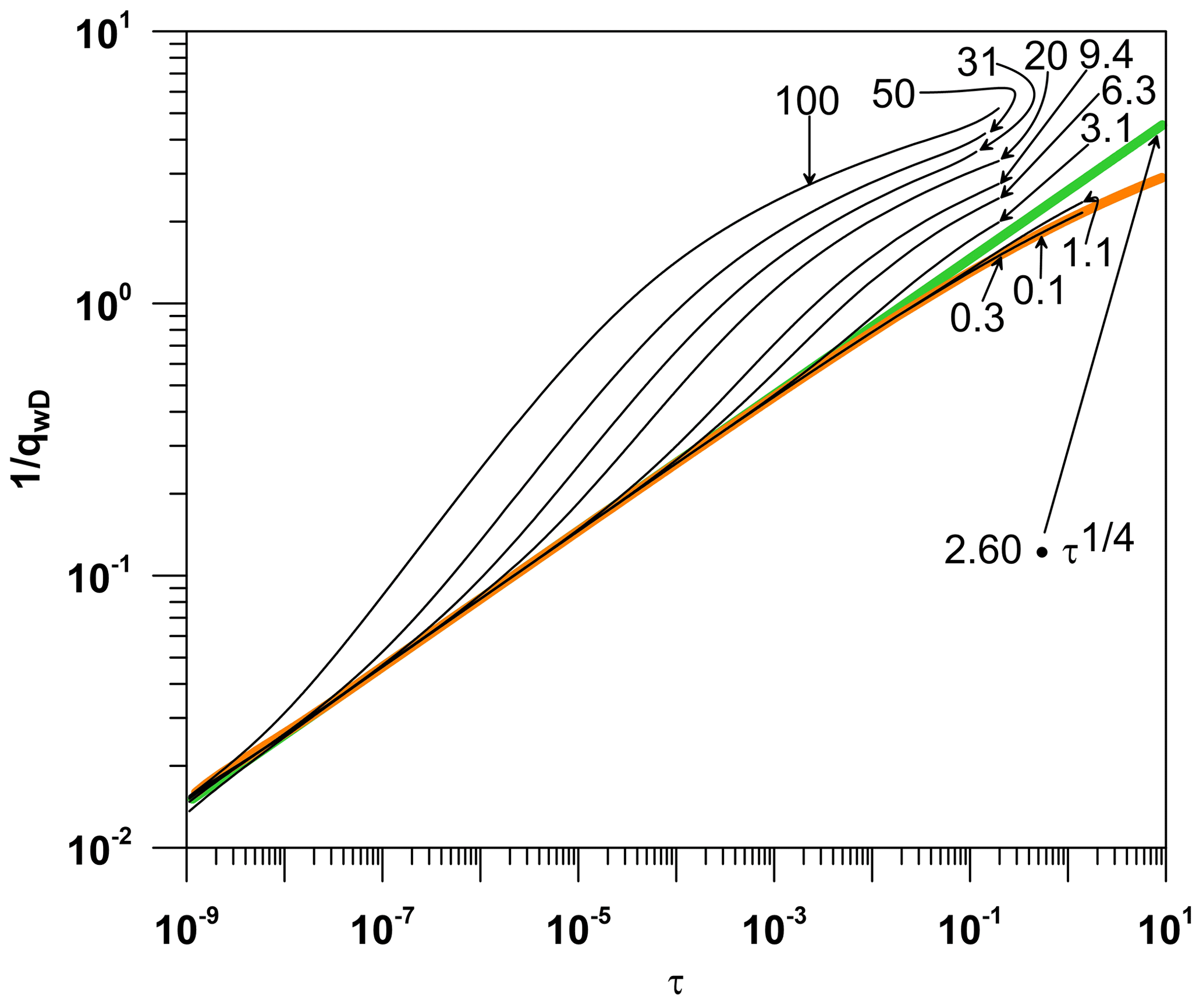
Figure 2 Model results displayed as 1∕q_wD vs. τ on a log–log scale. Bilinear fit curve (green line), master curve (orange line), and type curves (black lines).

3 Results

Numerical simulations show that during a time interval, the reciprocal of dimensionless flow rate in the well 1∕q_wD is proportional to the fourth root of dimensionless time τ^1∕4 (Fig. 2). This proportionality is in accordance with the behavior documented by Guppy et al. (1981b) and Silva-López et al. (2018). In particular, we can describe the variation in dimensionless flow rate in the well during the bilinear flow regime as

$$\begin{array}{}\text{(12)}& {\displaystyle \frac{\mathrm{1}}{q_{\mathrm{wD}}}}\left(\mathit{\tau }\right)=A\cdot {\mathit{\tau }}^{\mathrm{1}/\mathrm{4}},\end{array}$$

where the constant A is equal to 2.60. From now on, we will refer to this equation as the bilinear fit curve (green line in Fig. 2). Note that the coefficient A obtained by Guppy et al. (1981b) employing a semi-analytical solution is approximately A=2.722 (see Eq. 10). This slight difference between our and their result for A might be due to the temporal and spatial discretization utilized by them. The reciprocal of dimensionless flow rate exhibits a behavior proportional to the fourth root of time (Eq. 12), which is characteristic of bilinear flow regime; hence we can corroborate the occurrence of it.

We define the master curve as the one that describes the behavior of an infinitely long fracture (orange line in Fig. 2). The curves describing the behavior of the reciprocal of dimensionless flow rate over time for different dimensionless fracture conductivities, from T_D=0.1 up to T_D=100, are addressed as type curves (black lines in Fig. 2).

Taking into account all the aspects previously described, when type curves start departing from the bilinear fit curve (Fig. 2), this indicates that the transition from bilinear flow regime to formation linear flow regime (cases with high T_D) or to pseudo-radial flow regime (cases with low T_D) begins (Ortiz R. et al., 2013).

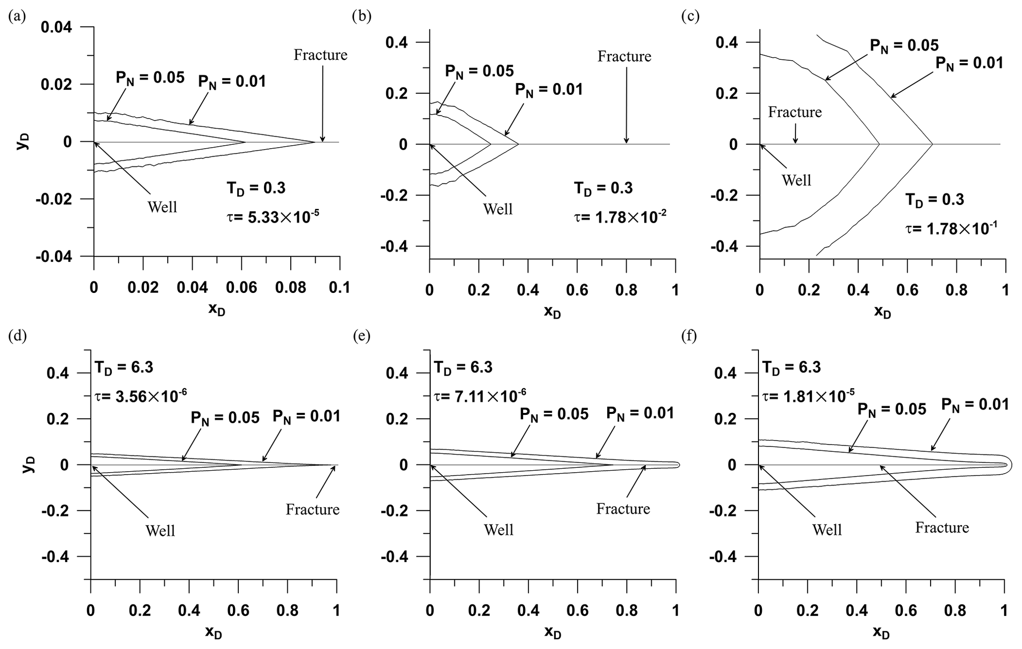
Figure 3 Spatial evolution of isobars P_N=0.01 and P_N=0.05 over time through the modeling domain, for the dimensionless fracture conductivities T_D=0.3 (a, b, c) and T_D=6.3 (d, e, f). Note that for the case of T_D=0.3, the scale of the graph (a) is different from that used for the graphs (b) and (c). Read text in Sect. 3.1 for a more detailed description of the graphs.

3.1 Propagation of isobars along the fracture and the formation

In order to characterize the different isobars, the following definition is used (Ortiz R. et al., 2013):

$$\begin{array}{}\text{(13)}& P_{\mathrm{N}}={\displaystyle \frac{p\left(x,y,t\right)-p_{\mathrm{i}}}{p_{\mathrm{w}}-p_{\mathrm{i}}}},\end{array}$$

where $p\left(x,y,t\right)$ denotes the pressure at the position (x,y) in the fracture or the matrix at time t. The values of P_N utilized in this study are 0.01 and 0.05, which are equivalent to the isobars of 109 and 145 kPa, respectively. The isobars behave differently depending on the value of T_D. For cases with low T_D, it is noticeable that after the termination of bilinear flow, the isobars reveal a tendency of progressing toward an elliptical or pseudo-radial flow while still propagating along the fracture (see, for example, T_D= 0.3 in Fig. 3a, b, c). The lower the value of T_D, the more pronounced this tendency becomes. On the other hand, for high T_D the behavior of the isobars is similar to the formation linear flow beyond the fracture (see T_D=6.3 in Fig. 3d, e, f). Although the behavior of isobars after the termination of bilinear flow is also highly interesting, this aspect is not addressed in further detail in this work. It remains to be studied in a follow-up investigation.

The results of this investigation show that initially the migration of isobars P_N along the fracture (see Fig. 1) is proportional to the fourth root of time:

$$\begin{array}{}\text{(14)}& x_{\mathrm{iD}}={\mathit{\alpha }}_{\mathrm{b}}{T}_{\mathrm{D}}{\mathit{\tau }}^{\mathrm{1}/\mathrm{4}},\end{array}$$

where x_iD represents the dimensionless distance of normalized isobars P_N from the well along the x_D axis and α_b is a constant that depends on the studied isobar P_N (see Fig. 4).

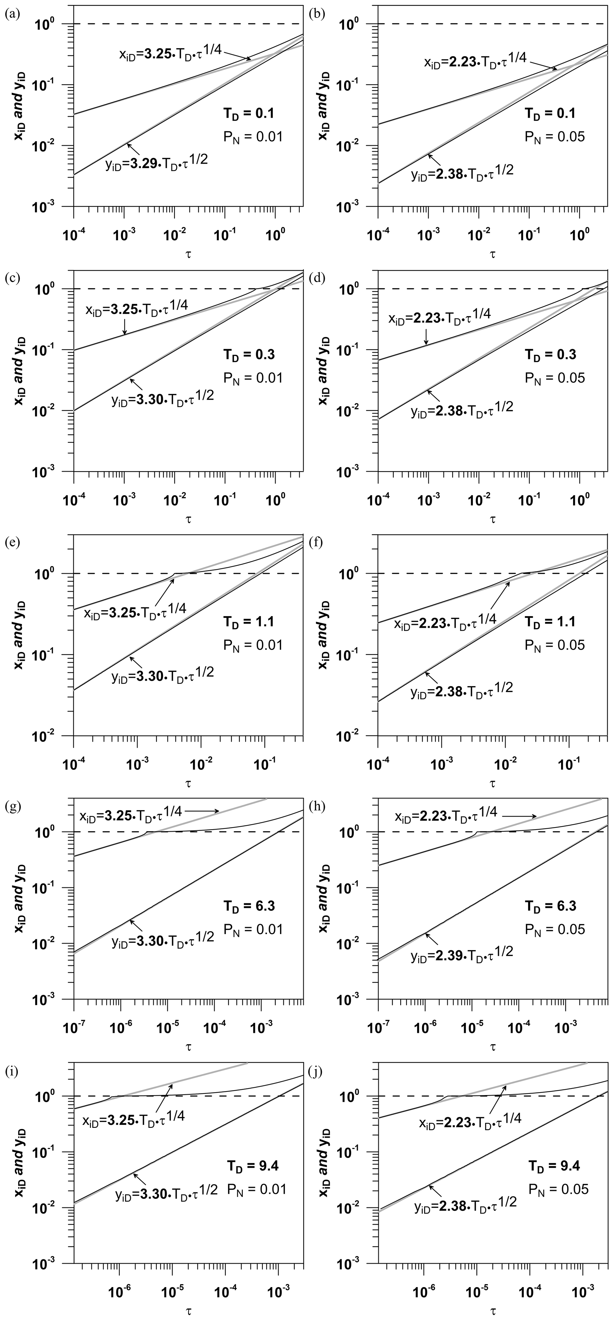
Figure 4 Model results display x_iD and y_iD vs. τ on a log–log scale. Propagation of isobars P_N=0.01 (a, c, e, g, i) and P_N=0.05 (b, d, f, h, j) along the fracture and the formation considering the following dimensionless fracture conductivities: T_D=0.1 (a, b), 0.3 (c, d), 1.1 (e, f), 6.3 (g, h), and 9.4 (i, j). The dashed lines represent the arrival at the fracture tip of the specific isobars indicated in the graphs.

In addition, the migration of isobars P_N in the matrix (perpendicular to the fracture and at x_D=0; see Fig. 1) for short times may be described by

$$\begin{array}{}\text{(15)}& y_{\mathrm{iD}}={\mathit{\alpha }}_{\mathrm{m}}{T}_{\mathrm{D}}{\mathit{\tau }}^{\mathrm{1}/\mathrm{2}},\end{array}$$

where y_iD denotes the dimensionless distance of normalized isobars P_N from the well along the y_D axis and α_m is a constant for pressure diffusion in the matrix, which depends on the isobar under investigation.

When expressing Eqs. (14) and (15) in dimensional form, for the x axis, Eq. (14) is given by

$$\begin{array}{}\text{(16)}& x_{\mathrm{i}}\left(t\right)={\mathit{\alpha }}_{\mathrm{b}}{\left(D_{\mathrm{b}}t\right)}^{\mathrm{1}/\mathrm{4}};\end{array}$$

and for the y axis, Eq. (15) is given by

$$\begin{array}{}\text{(17)}& y_{\mathrm{i}}\left(t\right)={\mathit{\alpha }}_{\mathrm{m}}{\left(D_{\mathrm{m}}t\right)}^{\mathrm{1}/\mathrm{2}}.\end{array}$$

In Eq. (17), $D_{\mathrm{m}}=k_{\mathrm{m}}/\left({\mathit{\eta }}_{\mathrm{f}}{s}_{\mathrm{m}}\right)$ (m² s⁻¹) is known as hydraulic diffusivity of matrix and is analogous to the definition of thermal diffusivity. Additionally, in Eq. (16) $D_{\mathrm{b}}=T_{\mathrm{F}}^{\mathrm{2}}/k_{\mathrm{m}}{\mathit{\eta }}_{\mathrm{f}}{s}_{\mathrm{m}}$ (m⁴ s⁻¹) is referred to as effective hydraulic diffusivity of fracture in a bilinear flow regime (Ortiz R. et al., 2013).

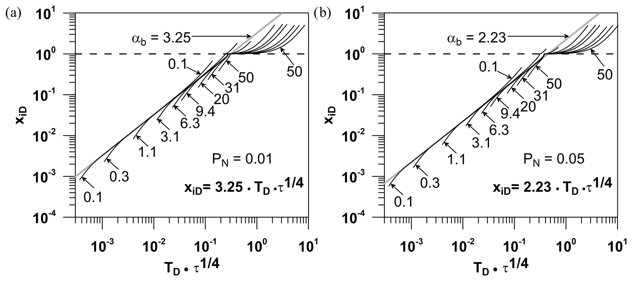
Figure 5 Model results in terms of x_iD vs. $T_{\mathrm{D}}\cdot {\mathit{\tau }}^{\mathrm{1}/\mathrm{4}}$ on a log–log scale. Propagation of isobars P_N along the fracture considering the following dimensionless fracture conductivities: T_D=0.1, 0.3, 1.1, 3.1, 6.3, 9.4, 20, 31, and 50. (a) Model scenarios with P_N=0.01 and α_b=3.25; (b) model scenarios with P_N=0.05 and α_b=2.23. The dashed lines represent the arrival at the fracture tip of the specific isobars indicated in the graphs.

The numerical results are specified as migration type curves (see black lines in Figs. 4, 5, and 6), and the fit equations for the propagation of isobars are referred to as migration fit curves (see grey lines in Figs. 4, 5, and 6). It can be noted qualitatively throughout the cases under study that for low dimensionless fracture conductivities, i.e., T_D=0.1 and T_D=0.3, the migration type curves, which describe the migration of isobars P_N along both the x_D and the y_D axis, start departing from migration fit curves before the studied isobars reach the fracture tip (Figs. 4a, b, c, d, and 5). In contrast, for the cases considering high dimensionless fracture conductivities, i.e., T_D=1.1, T_D=6.3, and T_D=9.4, there is no qualitative evidence of migration type curves departing from migration fit curves before the studied isobars P_N arrive at the fracture tip (Figs. 4e, f, g, h, i, j and 5). The latter results, however, show some exceptions for a slight acceleration exhibited by the isobars P_N at times shortly before they reach the fracture tip. It is important to mention that this relatively small acceleration also occurs for cases with low dimensionless fracture conductivities (see Fig. 4c, d). The same behavior was observed by Ortiz R. et al. (2013) for the injection at a constant flow rate. The classic definition for acceleration was considered, which is the rate of change of velocity with respect to time.

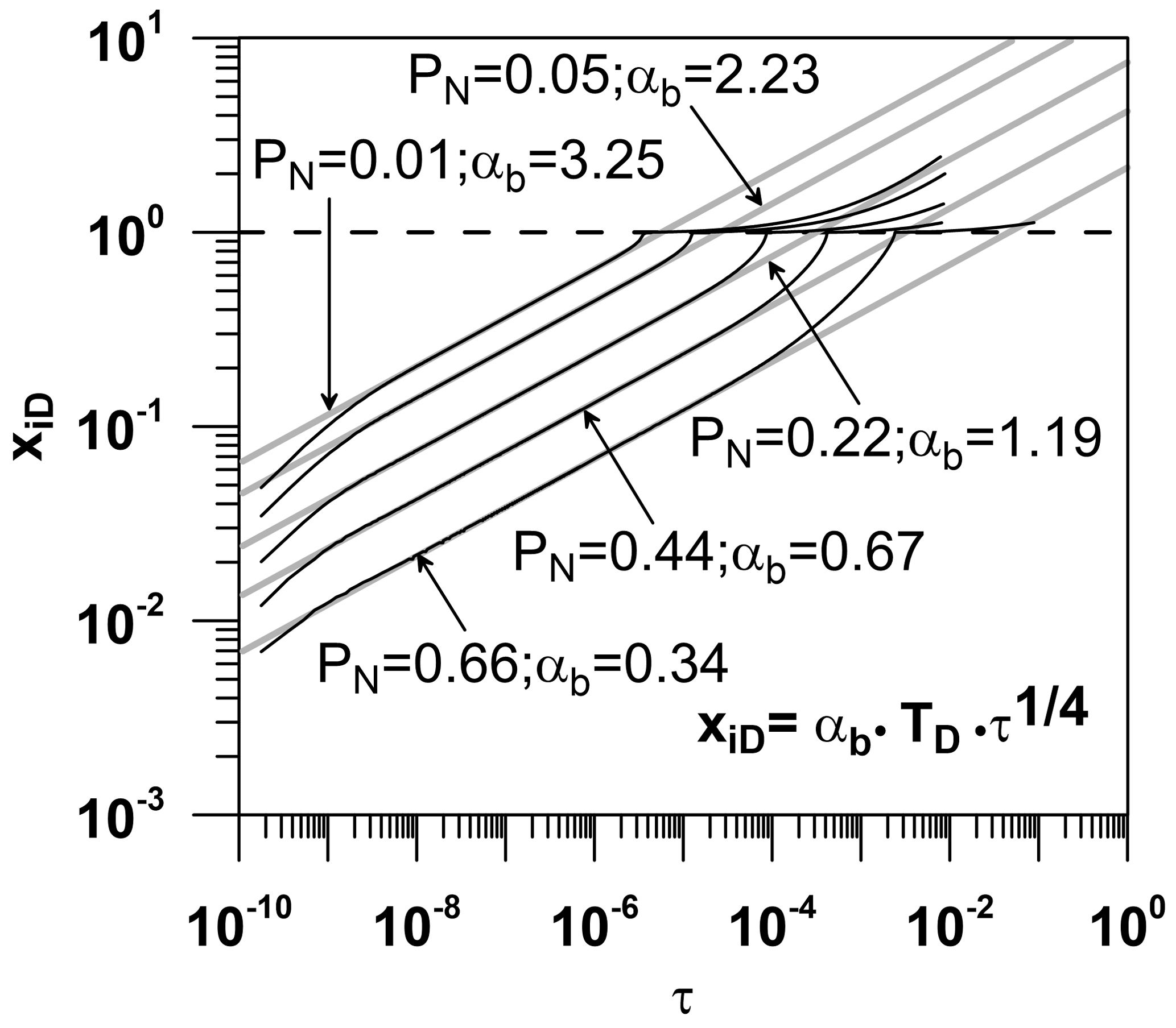
Figure 6 Modeling results in terms of x_iD vs. τ on a log–log scale. Propagation of isobars P_N=0.01, 0.05, 0.22, 0.44, and 0.66 with T_D=6.3. The dashed line represents the arrival at the fracture tip of the specific isobars indicated in the graph.

On the one hand, when discussing the early time qualitatively, we notice that the higher the value of the isobar P_N, the sooner it starts behaving proportional to the fourth root of time (Fig. 6). For example, at the same time ($\mathit{\tau }=\mathrm{5}\cdot {\mathrm{10}}^{-\mathrm{10}}$) the isobar P_N=0.66 (the greater isobar under investigation) starts to migrate along the fracture proportional to the fourth root of time, whereas the isobar P_N=0.01 (the smaller isobar under study) has not yet started to propagate proportionally to the fourth root of time. Moreover, the greater the isobar P_N, the shorter its distance from the well x_iD in comparison to other smaller isobars when considering the same time τ, which is logical since the isobars migrate one after the other. On the other hand, when discussing the long time qualitatively, we notice that the smaller isobar P_N=0.01 departs from the migration fit curve when it reaches the fracture tip. In contrast, the greater isobar P_N=0.66 departs from the migration fit curve before its arrival at the fracture tip (Fig. 6). Additionally, it can be seen that the higher the value of isobar P_N, the farther from the fracture tip or, closer to the well, it starts departing from the migration fit curve. Thus, taking into consideration the migration of isobars, it is reasonable to conclude that for high dimensionless fracture conductivities T_D, the bilinear flow regime ends when the pressure front reaches the fracture tip.

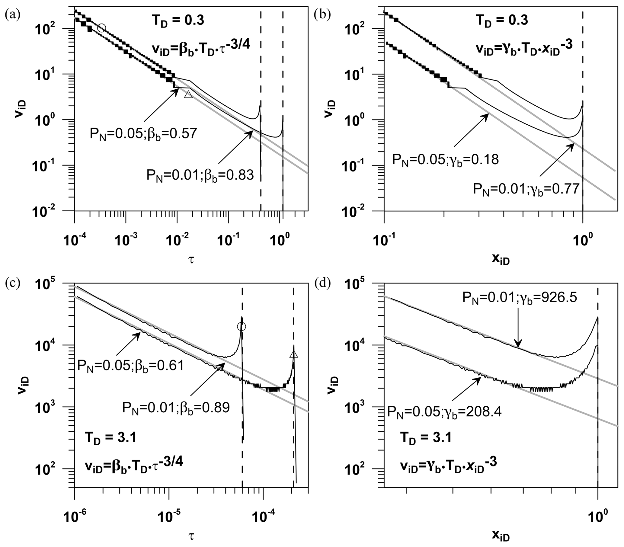
Figure 7 Model results showing v_iD vs. τ and v_iD vs. x_iD on a log–log scale. Velocity of isobars P_N=0.01 and 0.05 considering T_D=0.3 (a, b) and 3.1 (c, d). The dashed lines represent the arrival of the specific isobars at the fracture tip. (a) The circle and triangle symbols represent the transition time τ_t for P_N=0.01 and 0.05, respectively (see Eq. 20). (c) The circle and triangle symbols represent the arrival time τ_a for P_N=0.01 and 0.05, respectively (see Fig. 8).

Previously, we referred to the observation concerning the acceleration that isobars experience at times shortly before they arrive at the fracture tip (see Figs. 4, 6), which was also documented in Ortiz R. et al. (2013) for the case of fluid injection at a constant flow rate. To prove that it is truly an acceleration, the velocity of isobars is determined by calculating Δx_iD∕Δτ, and it is graphed versus time τ as well as versus the distance of isobars from the well x_iD (see Fig. 7). The existence of this acceleration in x_iD=1 (fracture tip; see Fig. 7) can be clearly seen. The velocity of isobars v_iD during their migration along the fracture decreases almost for the complete intervals of time considered (Fig. 7a, c), except for its evident increase at times shortly before the isobars reach the fracture tip. The velocity of isobars can be described within the intervals of time used as

$$\begin{array}{}\text{(18)}& v_{\mathrm{iD}}\left(\mathit{\tau }\right)={\mathit{\beta }}_{\mathrm{b}}{T}_{\mathrm{D}}{\mathit{\tau }}^{-\mathrm{3}/\mathrm{4}},\end{array}$$

where β_b is a constant that depends on the isobar under study. The velocity of isobars in terms of their distances from a well and within the ranges of distance used can be described as

$$\begin{array}{}\text{(19)}& v_{\mathrm{iD}}\left(x_{\mathrm{iD}}\right)={\mathit{\gamma }}_{\mathrm{b}}{T}_{\mathrm{D}}{x}_{\mathrm{iD}}^{-\mathrm{3}},\end{array}$$

where γ_b is a constant that depends on the isobar under study.

Before the isobars reach the fracture tip and at the same time τ, the velocity of isobar P_N=0.01 is higher than the velocity of P_N=0.05 (Fig. 7a, c). Furthermore, we can see that the arrival at the fracture tip of P_N=0.05 occurs after the arrival of P_N=0.01, what is also distinguishable in Figs. 4 and 6. The latter modeling results make sense since isobars migrate one after the other, P_N=0.01 first in the propagation along the fracture as it is the smallest among them. Moreover, before the arrival of isobars at the fracture tip and at a certain point belonging to the fracture, the velocity of the isobar P_N=0.01 is higher than the velocity of P_N=0.05 (Fig. 7b, d).

3.2 Termination of bilinear flow

Concerning the study related to the termination of bilinear flow considering fluid injection at a constant flow rate, Ortiz R. et al. (2013) introduced three criteria: the transition criterion, the reflection criterion, and the arrival criterion. The transition and reflection criteria take into account measurements of flow rate in the well, and the arrival criterion considers measurements of the migration of isobars P_N along the fracture. In this work, a fracture criterion is presented for the first time. This criterion quantifies the separation between the migration type curves and the migration fit curves (see Fig. 4). The time at which this separation occurs is defined as the fracture time. It is important to mention that only one criterion can be fulfilled at a time. To sum up, there exist two methodologies to quantitatively identify the termination of bilinear flow: (a) considering the transition of the pressure or flow rate in the well and (b) considering the propagation of isobars P_N along the fracture. It is noteworthy that the termination time is referred to differently, according to the criterion used to identify the time at which the bilinear flow regime ceases (e.g., transition time τ_t, reflection time τ_r, arrival time τ_a, and fracture time τ_F, introduced in Sect. 3.2.1, 3.2.2, 3.2.3, and 3.2.4, respectively). Further, criteria generally aim to define the deviation of curves obtained by numerical simulations from analytical fit curves that correspond to bilinear flow. The deviation is quantified by introducing the quantity ε (see Sect. 3.2.1, 3.2.2, and 3.2.4). That is, the numerical results differ from the analytical bilinear fit curves by a value of ε due to the transition to another flow regime. Throughout the paper we use, for instance, ε=0.01 or ε=0.05 corresponding to 1 % and 5 % deviation, respectively. That means when a separation between numerical results and fit curves is greater than 0.01 or 0.05, the termination of bilinear flow is identified.

3.2.1 Transition criterion

This criterion quantifies the clockwise deviation of type curves from the bilinear fit curve in Fig. 2, and it is fundamentally utilized for low dimensionless fracture conductivities of T_D=1.1 down to T_D=0.1:

$$\begin{array}{}\text{(20)}& \mathit{\epsilon }<\mathrm{1}-\left({\displaystyle \frac{\log \left(\frac{\mathrm{1}}{q_{\mathrm{wDt}}}\right)}{\log \left(\mathrm{2.60}{\mathit{\tau }}^{\mathrm{1}/\mathrm{4}}\right)}}\right),\end{array}$$

where q_wDt represents the dimensionless flow rate q_wD of the specific type curve under study (Fig. 2). Note that 1∕q_wD vs. τ is associated with equation 2.60τ^1∕4 on a log–log plot (bilinear fit curve). The cases to which this criterion is applied are not affected by the fracture tip, and the transition time is similar for all type curves for which this criterion is suitable (see τ_t in Fig. 8). The transition time τ_t defines the end of bilinear flow when 1∕q_w is no longer proportional to t^1∕4.

3.2.2 Reflection criterion

The reflection criterion quantifies the counterclockwise deviation of type curves from the master curve in Fig. 2 due to isobar reflection at the fracture tip (Ortiz R. et al., 2013). When lower isobars than the isobar under study have already reached the fracture tip, these isobars are partly reflected from the fracture tip toward the well, due to the hydraulic conductivity contrast experienced at the interphase between the fracture tip and the matrix. This hydraulic conductivity structure causes the isobar reflection at the fracture tip to move back toward the well and the isobar transmission further into the matrix. Thus, the propagation velocity of all isobars decelerates when they leave the fracture tip and start to propagate through the matrix. This criterion is used for high dimensionless fracture conductivities:

$$\begin{array}{}\text{(21)}& \mathit{\epsilon }<\mathrm{1}-\left({\displaystyle \frac{\log \left(\frac{\mathrm{1}}{q_{\mathrm{wD}\mathrm{\infty }}}\right)}{\log \left(\frac{\mathrm{1}}{q_{\mathrm{wDt}}}\right)}}\right),\end{array}$$

where q_wD∞ denotes the dimensionless flow rate of the master curve (Fig. 2), which describes the behavior for the case of an infinitely long fracture. The cases to which this criterion is applicable are affected by the fracture tip; hence the higher T_D, the shorter the reflection time (see τ_r in Fig. 8). The reflection time τ_r refers to the time at which a first variation in pressure is evident in the fracture tip.

3.2.3 Arrival criterion

The arrival criterion represents the moment at which the isobars arrive at the fracture tip. The cases to which this criterion is applicable are affected by the fracture tip; hence the higher T_D, the shorter the arrival time (see τ_a in Fig. 8).

3.2.4 Fracture criterion

Basically, the fracture criterion states that the separation between the migration type curves and the migration fit curves (see Fig. 4) is representative of the end of bilinear flow regime, and it is applicable to low dimensionless fracture conductivities. In this work, the propagation along y_D is not a criterion for the termination of bilinear flow; it is only a contribution to the study of its behavior. Usually, for the analysis of bilinear flow at constant injection or production flow rate the transient wellbore pressure is studied; thus the bilinear flow occurs when the wellbore pressure is proportional to the fourth root of time (Cinco-Ley and Samaniego-V., 1981; Ortiz R. et al., 2013; Weir, 1999). Similarly, for constant wellbore pressure as in this work, the bilinear flow can be recognized by the proportionality between 1∕q_wD and τ^1∕4. The fracture criterion, instead of considering the variation in 1∕q_wD vs. time in the well, quantifies the separation of migration type curves from migration fit curves (Fig. 4), and it is defined as

$$\begin{array}{}\text{(22)}& \mathit{\epsilon }<\mathrm{1}-\left({\displaystyle \frac{\log \left(x_{\mathrm{iDf}}\right)}{\log \left(x_{\mathrm{iDt}}\right)}}\right),\end{array}$$

where x_iDf and x_iDt represent the propagation of the migration fit curves and the migration type curves, respectively. The latter have the form α_bT_Dτ^1∕4 (see Eq. 14 and Fig. 4). The cases to which this criterion is applied are not affected by the fracture tip, and the fracture time is similar for all migration type curves for which this criterion is suitable (see τ_F in Fig. 8). Summarizing, this criterion takes into consideration only the movement of isobars P_N along the fracture and not the change of 1∕q_wD in the well, and it is suitable for low dimensionless fracture conductivities T_D.

In the framework of this study, when we consider the transition of flow rate in the well, the criteria that can be utilized are the transition criterion (see Sect. 3.2.1) and the reflection criterion (see Sect. 3.2.2). When we consider the propagation of isobars along the fracture, the criteria that can be used are the arrival criterion (see Sect. 3.2.3) and the fracture criterion (see Sect. 3.2.4).

Despite the values for the transition criterion and the fracture criterion being different, their behaviors are similar. They present almost constant values within the range of T_D in which these criteria are applied. Note that the values of the fracture criterion are always higher than the values of the transition criterion. The fracture criterion can give us a reliable estimate of the termination of bilinear flow when considering the low dimensionless fracture conductivities T_D for which this criterion is applicable. The transition and fracture criteria make sense only until the isobars P_N reach the fracture tip (see Fig. 8).

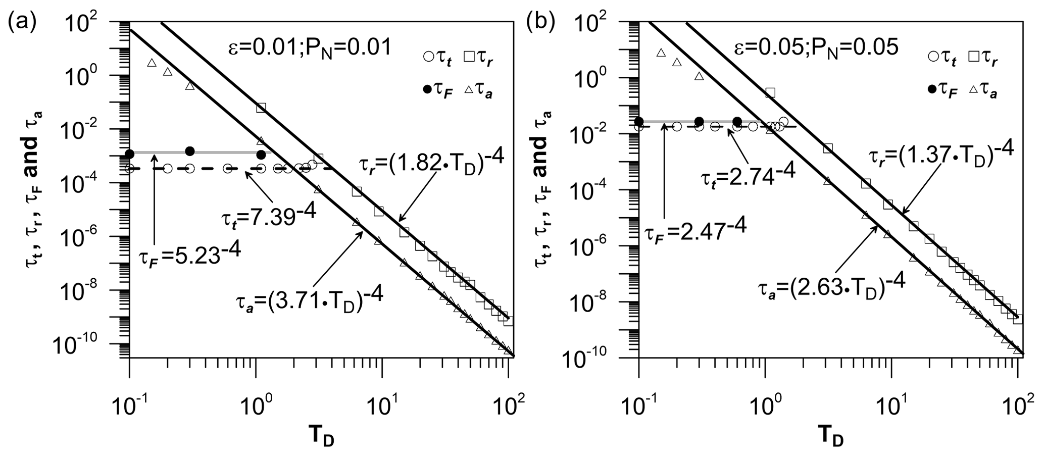
Figure 8 Model results displaying τ_t, τ_r, τ_F, and τ_a vs. T_D on a log–log scale. τ_t, τ_r, τ_F, and τ_a denote the transition time, the reflection time, the fracture time, and the arrival time, respectively. The fit curves for reflection time and arrival time are represented by black lines, for transition time by dashed lines, and for fracture time by grey lines. (a) Numerical simulations with ε and P_N=0.01; and (b) numerical simulations with ε and P_N=0.05 (see Eqs. 20, 21, and 22).

As we showed earlier, it does not make sense to discuss the occurrence of bilinear flow after the pressure front has already arrived at the fracture tip. Nevertheless, the results show (Fig. 8) that the reflection time τ_r (related to the flow rate calculated in the well) is greater than the arrival time τ_a (related to the moment at which the isobars reach the fracture tip). It means that the reciprocal of dimensionless flow rate calculated in the well is proportional to the fourth root of time even when the pressure front has already reached the fracture tip.

4 Discussion

Dimensionless time was not defined using the conventional definition t_D; instead, a modified definition τ presented by Ortiz R. et al. (2013) was used. It turned out to be convenient in terms of interpreting the results for bilinear flow since it was possible to graph the behavior of 1∕q_wD vs. τ for all dimensionless fracture conductivities T_D in the same graph (Fig. 2).

As for the comparison between the coefficient A=2.6 obtained by us (Eq. 12) and the coefficient A=2.772 documented by Guppy et al. (1981b), we can observe a discrepancy between these results of approximately 6 %. This discrepancy can be considered rather low.

Some type curves bend clockwise and some others bend counterclockwise from the bilinear fit curve (Fig. 2). Among the cases of dimensionless fracture conductivities T_D studied, the type curves that bend clockwise are T_D=0.1, 0.3 and 1.1, and those that bend counterclockwise are T_D=3.1, 6.3, 9.4, 20, 31, 50, and 100. Similar results were obtained by Ortiz R. et al. (2013) for the case of injection at a constant flow rate. For the interval of time utilized in the simulation, the behavior of 1∕q_wD versus τ for dimensionless fracture conductivities T_D=0.1 and 0.3 is identical to the behavior of an infinitely long fracture (master curve, orange line in Fig. 2) since the separation of the mentioned type curves from the master curve should occur at a time greater than the simulation time utilized here.

Our results concerning the propagation of isobars along the fracture and the matrix (Eqs. 14, 15) are similar to the results previously presented by Ortiz R. et al. (2013) regarding the migration of isobars. The values of α_b obtained by us for P_N=0.01 and 0.05 are quantitatively different from the values documented by them in 4.6 % and 5.8 %, respectively.

At times, shortly before the isobars reach the fracture tip, they exhibit an acceleration along the fracture (see Figs. 4, 6). Subsequently, once the isobars arrive at the fracture tip, they no longer progress through the matrix over a certain period of time. Afterward, they experience another acceleration along the fracture, with which the migration of isobars seems to approach a propagation proportional to the square root of time (see Fig. 4). An identical behavior was observed by Ortiz R. et al. (2013), and they attributed it to the reflection of isobars at the fracture tip, which makes sense and could be confirmed in this study. The acceleration nearby the fracture tip can be observed more clearly when analyzing the velocity along the fracture (see Fig. 7b, d). During the intervals of time used, the migration of isobars along the fracture experiences a constant deceleration, except when they approach the fracture tip. This deceleration is qualitatively identical for P_N=0.01 and P_N=0.05 (see Fig. 7a, c). It is evident that for all fixed dimensionless positions in the fracture and considering the same dimensionless fracture conductivity T_D, the velocity v_iD is higher for low values of normalized isobars P_N (see Fig. 7b, d). One reason of this observation is that once the deceleration begins, P_N=0.01 propagates faster than P_N=0.05 since the initial velocity (when the isobar leaves the well) of the isobar P_N=0.01 is higher than the initial velocity of the isobar P_N=0.05. This behavior is explained based on the fact that the pressure gradient between the well and the fracture is bigger when P_N=0.01 is leaving the well than when P_N=0.05 is leaving it. Furthermore, for all fixed dimensionless positions in the fracture and considering the same isobar P_N, the velocity v_iD is higher for high dimensionless fracture conductivities (see Fig. 7b, d).

Using Eqs. (18) and (19), the migration of isobars along the fracture can be described as

$$\begin{array}{}\text{(23)}& x_{\mathrm{iD}}={\left({\displaystyle \frac{{\mathit{\beta }}_{\mathrm{b}}}{{\mathit{\gamma }}_{\mathrm{b}}}}\right)}^{-\mathrm{1}/\mathrm{3}}{\mathit{\tau }}^{\mathrm{1}/\mathrm{4}}.\end{array}$$

Note that Eq. (23) has the same form that Eq. (14); thus

$$\begin{array}{}\text{(24)}& {\left({\displaystyle \frac{{\mathit{\beta }}_{\mathrm{b}}}{{\mathit{\gamma }}_{\mathrm{b}}}}\right)}^{-\mathrm{1}/\mathrm{3}}={\mathit{\alpha }}_{\mathrm{b}}{T}_{\mathrm{D}}.\end{array}$$

It is possible to verify the validity of Eq. (24) by introducing the required values.

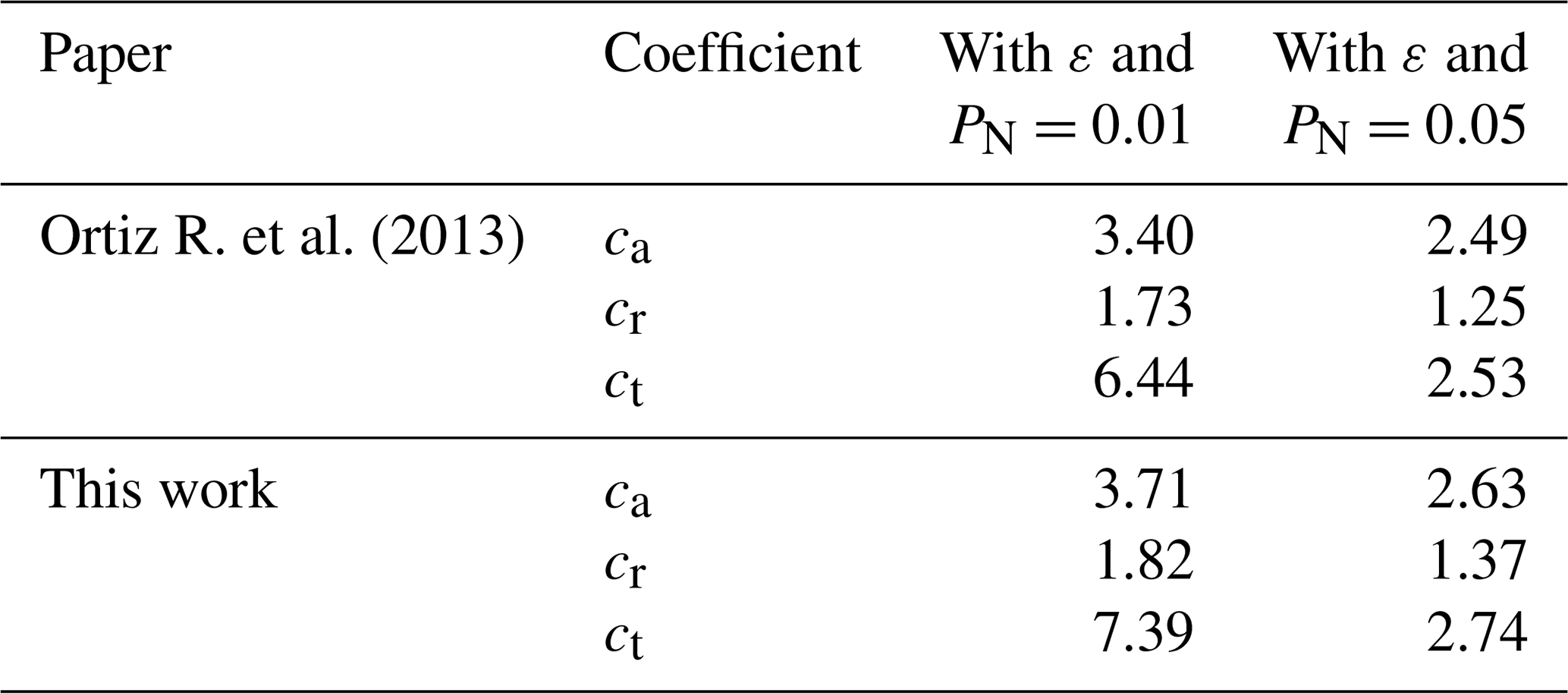
For the case of injection at a constant flow rate the results obtained by Ortiz R. et al. (2013) for the arrival time, the reflection time, and the transition time are similar to ours (see Table 1). It is worth noting that when using the expression ε and P_N=0.01, it means that we are studying the case of the isobar P_N=0.01, and we consider that for values of ε greater than 0.01, the bilinear flow ends. Note further that when considering ε and P_N=0.05, we are studying the isobar P_N=0.05 and we are using a value of ε=0.05 to determine the termination of bilinear flow, for all pertinent criteria.

Table 1 Comparison of coefficients of fit equations for the arrival time, the reflection time, and the transition time, which have the form ${\mathit{\tau }}_{\mathrm{a}}={\left(c_{\mathrm{a}}\cdot T_{\mathrm{D}}\right)}^{-\mathrm{4}}$, ${\mathit{\tau }}_{\mathrm{r}}={\left(c_{\mathrm{r}}\cdot T_{\mathrm{D}}\right)}^{-\mathrm{4}}$, and ${\mathit{\tau }}_{\mathrm{t}}={\left(c_{\mathrm{t}}\right)}^{-\mathrm{4}}$, respectively (see Fig. 8).

When it comes to the criteria that consider the transition of 1∕q_wD some observations can be made: (a) in the case of Fig. 8a the transition criterion is fulfilled up to a value of T_D approximately of 2 and for values of T_D above 3 the reflection criterion is fulfilled; and (b) in the case of Fig. 8b the transition criterion is fulfilled up to a value of T_D of approximately 1.1 and for values of T_D above 2 the reflection criterion is fulfilled. Note that for the case ε and P_N=0.01 and $\mathrm{2}<T_{\mathrm{D}}<\mathrm{3}$ (see Fig. 8a), it is observed that values (non-filled circles) depart from the fit curve linked to the transition criterion and start converging toward the fit curve associated with the reflection criterion. A similar behavior is also observed for the case ε and P_N=0.05 and $\mathrm{1.1}<T_{\mathrm{D}}<\mathrm{2}$ (see Fig. 8b). A comprehensive study is required to unravel more precisely what occurs within those ranges of T_D. Based on their work, Ortiz R. et al. (2013) came to the same conclusion.

Ultimately, there are two ways to determine the termination of bilinear flow: (I) by numerically measuring the transient flow rate in the well and obtaining the transition time τ_t for low T_D and the reflection time τ_r for high T_D and (II) according to the migration of isobars along the fracture (not measurable in the well), obtaining the fracture time τ_F for low T_D and the arrival time τ_a for high T_D (see Table 2).

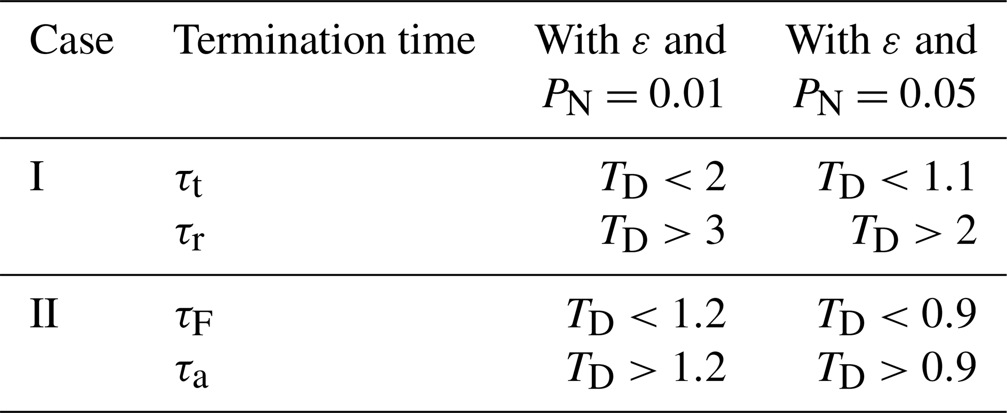
Table 2 Criteria utilized to calculate the termination of bilinear flow. See discussion for the definition of the cases I and II.

In a follow-up study, it would be interesting to include the effect of fracture storativity and, utilizing an analogue method to that discussed in this work, investigate the behavior of a fracture with conductivity high enough to lead to fracture and formation linear flow.

Application to well testing problems

In practical terms, when analyzing the transient flow rate in a well, only the transition time τ_t and the reflection time τ_r can be determined. With the current field methods, it is not possible to determine the termination of bilinear flow utilizing the progress of the pressure front along the fracture, although this is more physically reasonable. Nevertheless, the fracture length can be constrained indirectly, for instance by computing the time at which the pressure arrives at the fracture tip and its relation with respect to the reflection time. The relation between the arrival time τ_a and the reflection time τ_r is given by

$$\begin{array}{}\text{(25)}& {\mathit{\tau }}_{\mathrm{a}}\cong \mathrm{0.0579}{\mathit{\tau }}_{\mathrm{r}}\end{array}$$

for ε and P_N=0.01 (see Fig. 8a), and

$$\begin{array}{}\text{(26)}& {\mathit{\tau }}_{\mathrm{a}}\cong \mathrm{0.0736}{\mathit{\tau }}_{\mathrm{r}}\end{array}$$

for ε and P_N=0.05 (see Fig. 8b).

In the following, we present two artificial cases in which synthetic curves were constructed to illustrate how the measurements of the flow rate in wells during hydraulic tests at constant pressure are used to estimate or restrict the length of fractures with finite hydraulic conductivity (bilinear flow). The synthetic curves are not obtained from measurements of realistic well tests but computed utilizing the validated model concerning fractured porous geologic media, included in COMSOL Multiphysics^® and in previous papers.

Scenario A: high dimensionless fracture conductivities T_D

We proceed to elaborate a method to estimate the fracture length using measurements of the flow rate in the well. This is motivated by its usefulness for cases with high T_D in which the reflection criterion is applicable, i.e., provided that the isobar that is under study reaches the fracture tip while bilinear flow is still in progress. In this example, the values of the dimensional fracture conductivity T_F as well as the fracture length 2x_F are restricted by a synthetic curve representing the transient flow rate in the well. The synthetic curve is performed assuming that p_w=1 MPa, p_i=100 kPa, k_m=1 µD, $T_{\mathrm{F}}=\mathrm{1.5}\times {\mathrm{10}}^{-\mathrm{16}}$ m³, $s_{\mathrm{m}}={\mathrm{10}}^{-\mathrm{11}}$ Pa⁻¹, ${\mathit{\eta }}_{\mathrm{F}}=\mathrm{2.5}\times {\mathrm{10}}^{-\mathrm{4}}$ Pa s, and x_F=23.81 m (see Fig. 9). The procedure is described in series of steps as follows:

1. Dimensionally graphing the reciprocal of flow rate vs. time. It is worthwhile noting that the counterclockwise separation of the synthetic curve (red line) from the bilinear fit curve (grey line) represents the moment of arrival of the pressure front at the fracture tip, defining the end of bilinear flow.

2. Calculate T_F as is typically done (see, e.g., Guppy et al., 1981b), i.e., based on the slope of bilinear fit curve $\mathrm{1}/q_{\mathrm{w}}=m{t}^{\mathrm{1}/\mathrm{4}}$ (Eq. 12). The dimensional fracture conductivity is determined as follows:

   $$\begin{array}{}\text{(27)}& T_{\mathrm{F}}={\left({\displaystyle \frac{\mathrm{2.61}{\mathit{\eta }}_{\mathrm{F}}^{\mathrm{3}/\mathrm{4}}}{k_{\mathrm{m}}^{\mathrm{1}/\mathrm{4}}{s}_{\mathrm{m}}^{\mathrm{1}/\mathrm{4}}h(p_{\mathrm{w}}-p_{\mathrm{i}})m}}\right)}^{\mathrm{2}}.\end{array}$$

   According to this example, T_F is obtained as $\mathrm{1.5}\times {\mathrm{10}}^{-\mathrm{16}}$ m³. This value is the same as the one employed to perform the synthetic curve.

3. Read from the graph the termination of bilinear flow defined by the separation of the curve that represents the 1∕q_w measured in the well (red curve) from the curve proportional to t^1∕4 (grey curve). This time corresponds to the reflection time. In practical terms, it is considered a calculation error in the separation of 5 %, which corresponds approximately to the visual estimation of the point at which these curves start departing from each other. In this case study, the reflection time t_r is approximately 10⁴ s.

4. Introduce the value of reflection time t_r calculated in the previous step in the relation τ_a≅0.0736τ_r and obtain the arrival time of the isobars at the fracture tip. For the example at hand, t_a=736 s.

5. Determine the value of D_b from its definition:

   $$\begin{array}{}\text{(28)}& D_{\mathrm{b}}={\displaystyle \frac{T_{\mathrm{F}}^{\mathrm{2}}}{k_{\mathrm{m}}{\mathit{\eta }}_{\mathrm{F}}{s}_{\mathrm{m}}}}.\end{array}$$

   For the present case study, taking into account the example and the parameters of the simulation, D_b is obtained as 9 m⁴ s⁻¹.

   Introduce the value of t_a, obtained at step 4, and the value of D_b, calculated at step 5, in the equation of migration of isobars along the fracture (Eq. 16), and, in this way, calculate the fracture half-length. In this case, the isobar under study is P_N=0.05; as a result the constant α_b=2.23. Utilizing Eq. (16), we have

   $$\begin{array}{}\text{(29)}& x_{\mathrm{F}}={\mathit{\alpha }}_{\mathrm{b}}{\left(D_{\mathrm{b}}{t}_{\mathrm{a}}\right)}^{\mathrm{1}/\mathrm{4}}.\end{array}$$

   When introducing the corresponding values of the considered example, x_F is obtained as 20.12 m.

6. Finally, the fracture length is approximately 40.24 m (2x_F). It can be noted that this result is slightly lower than 47.62 m, which is the value that denotes the real magnitude used to represent the synthetic curve. It is possible to obtain more accurate results by quantitatively calculating the separation between the curves of the considered example instead of visually estimating it. For instance, when calculating explicitly a counterclockwise 5 % separation of the synthetic curve (red line) from the bilinear fit curve (grey line), an arrival time of 865.5 s and a fracture length of 41.9 m are obtained.

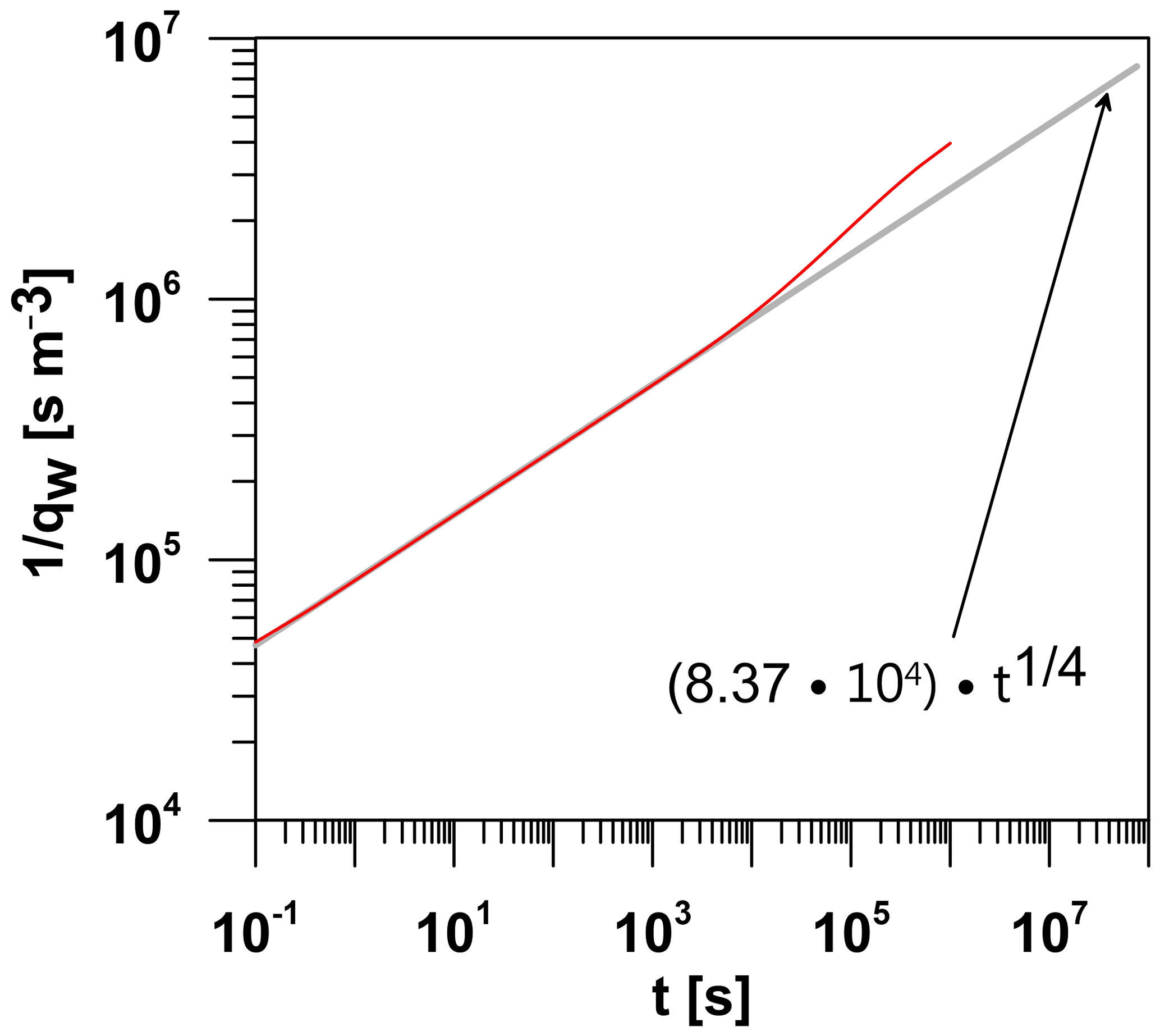
Figure 9 1∕q_w (s m⁻³) vs. t (s) on a log–log scale. The synthetic curve is represented by the red line and the bilinear fit curve is displayed with the grey line.

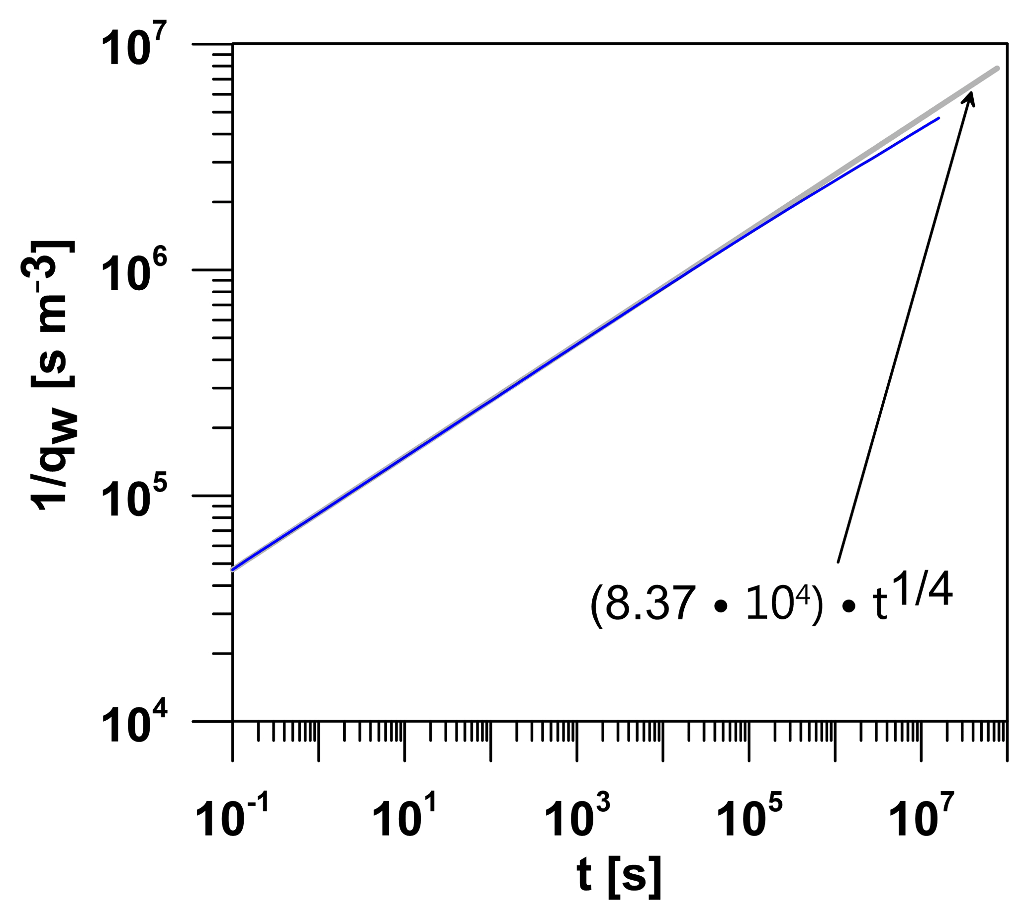
Figure 10 1∕q_w (s m⁻³) vs. t (s) on a log–log scale. The synthetic curve is represented by the blue line and the bilinear fit curve is indicated with the grey line.

Scenario B: low dimensionless fracture conductivities T_D

In the case of low T_D, it is not possible to estimate the fracture length utilizing the bilinear flow theory, since this flow regime ends before the isobar under study arrives at the fracture tip. This is expressed in terms of the pressure field by the observation of the premature occurrence of a significant pressure change in the fracture tip. However, it is possible to restrict the minimum fracture length. In the following example, the values of the dimensional fracture conductivity T_F as well as the minimum fracture length 2x_F are constrained by a synthetic curve representing the transient flow rate in the well. This latter curve is computed assuming that p_w=1 MPa, p_i=100 kPa, k_m=1 µD, $T_{\mathrm{F}}=\mathrm{1.5}\times {\mathrm{10}}^{-\mathrm{16}}$ m³, $s_{\mathrm{m}}={\mathrm{10}}^{-\mathrm{11}}$ Pa⁻¹, ${\mathit{\eta }}_{\mathrm{F}}=\mathrm{2.5}\times {\mathrm{10}}^{-\mathrm{4}}$ Pa s, and x_F=136.36 m (see Fig. 10). The procedure is outlined in the following steps:

1. Dimensionally graphing the reciprocal of flow rate vs. time.

2. Calculate the value of T_F as commonly conducted in the related literature (see, e.g., Guppy et al., 1981b), i.e., based on the slope of bilinear fit curve $\mathrm{1}/q_{\mathrm{w}}=m{t}^{\mathrm{1}/\mathrm{4}}$ (Eq. 12). The dimensional fracture conductivity is determined as follows:

   $$\begin{array}{}\text{(30)}& T_{\mathrm{F}}={\left({\displaystyle \frac{\mathrm{2.61}{\mathit{\eta }}_{\mathrm{F}}^{\mathrm{3}/\mathrm{4}}}{k_{\mathrm{m}}^{\mathrm{1}/\mathrm{4}}{s}_{\mathrm{m}}^{\mathrm{1}/\mathrm{4}}h(p_{\mathrm{w}}-p_{\mathrm{i}})m}}\right)}^{\mathrm{2}}.\end{array}$$

   According to this example, T_F is obtained as $\mathrm{1.5}\times {\mathrm{10}}^{-\mathrm{16}}$ m³. This value is the same as the one used to calculate the synthetic curve.

3. Read from the graph the termination of bilinear flow defined by the clockwise separation of the curve that represents the 1∕q_w measured in the well (blue curve) from the curve proportional to t^1∕4 (grey curve). This time is defined as transition time, and it is similar for all cases with low T_D. Similar to the previous case, a calculation error in the separation of 5 % is considered, which corresponds approximately to the visual estimation of the point at which both curves start departing from each other. In this example, the transition time t_t is approximately 10⁶ s.

4. Introduce the value of transition time t_t, calculated in the previous step, in the relation τ_a≅0.0736τ_t and obtain the fictitious arrival time of the isobars at the fracture tip. For the contemplated case example, t_a=73 600 s.

5. Determine the value of D_b from its definition:

   $$\begin{array}{}\text{(31)}& D_{\mathrm{b}}={\displaystyle \frac{T_{\mathrm{F}}^{\mathrm{2}}}{k_{\mathrm{m}}{\mathit{\eta }}_{\mathrm{F}}{s}_{\mathrm{m}}}}.\end{array}$$

   In the context of the example at hand and considering the parameters of the simulation, D_b is obtained as 9 m⁴ s⁻¹.

   Introduce the value of t_a, obtained at step 4, and the value of D_b computed at step 5, in the equation of migration of isobars along the fracture (Eq. 16) and, in this way, calculate the fictitious fracture half-length. In this case, the isobar under study is P_N=0.05; as a consequence the constant α_b=2.23. Utilizing Eq. (16) we have

   $$\begin{array}{}\text{(32)}& x_{\mathrm{F}}={\mathit{\alpha }}_{\mathrm{b}}{\left(D_{\mathrm{b}}{t}_{\mathrm{a}}\right)}^{\mathrm{1}/\mathrm{4}}.\end{array}$$

   When incorporating the corresponding values of this example, x_F is obtained as 63.62 m.

6. Finally, the minimum fracture length is approximately 127.23 m (2x_F), whereas the real value used to represent the synthetic curve is 272.72 m.

In the cases described previously, the practical use of Eq. (16) to constrain the length of a fracture with finite conductivity has been demonstrated by analyzing the transient behavior of flow rate in the well during a hydraulic test at constant pressure.

The expressions obtained in this work for the end time of bilinear flow, the pressure propagation, and the bilinear diffusivity D_b complement the limited theory that exists about data analysis from wells producing or injecting at constant pressure. The clarity and simplicity of these equations allow these to be used quickly to estimate the length of fractures with finite conductivity. The bilinear diffusivity D_b, first introduced by Ortiz R. et al. (2013) for constant well flow rate and demonstrated in this work to also hold for the case of constant well pressure, could in principle be estimated in the laboratory by means of Eq. (16). In addition, this bilinear diffusivity allows, on the one hand, for a relatively uncomplicated comparison between finite-conductivity fractures. On the other hand, these equations could in one way or another be integrated into more general methods such as the transient rate analysis for the interpretation of production data. Finally, the diffusivity equations of pressure in the matrix and the fracture (Eqs. 16, 17) are also useful to reduce the associated risks related to induced seismicity generated by changes of pressure in fractured reservoirs or faults, as a consequence of massive fluid injection (e.g. Shapiro, 2015; Shapiro and Dinske, 2009). By knowing and understanding the physics behind the migration of isobars it is possible to minimize the associated risks with changes in pores pressure.

5 Conclusions

Numerical results obtained in this work corroborated the relation of proportionality previously presented by Guppy et al. (1981b) between the reciprocal of dimensionless flow rate 1∕q_wD and the fourth root of dimensionless time τ during the bilinear flow regime for the case of injection at constant pressure in the well. Guppy et al. (1981b) obtained the proportionality factor A = 2.722 (Eq. 10), which is slightly greater than the factor obtained here A = 2.60 (Eq. 12). This discrepancy may be attributed to our finer spatial and temporal discretization in comparison with the discretization used by Guppy et al. (1981b).

The most significant findings of this work are as follows:

• i.

  During the bilinear flow regime, the migration of isobars along the fracture is described as $x_{\mathrm{i}}\left(t\right)={\mathit{\alpha }}_{\mathrm{b}}(D_{\mathrm{b}}t{)}^{\mathrm{1}/\mathrm{4}}$, where $D_{\mathrm{b}}=T_{\mathrm{F}}^{\mathrm{2}}/k_{\mathrm{m}}{\mathit{\eta }}_{\mathrm{f}}{s}_{\mathrm{m}}$ (m⁴ s⁻¹) is the effective hydraulic diffusivity of fracture during the bilinear flow regime. In addition, the migration of isobars in the matrix is given by $y_{\mathrm{i}}\left(t\right)={\mathit{\alpha }}_{\mathrm{m}}(D_{\mathrm{m}}t{)}^{\mathrm{1}/\mathrm{2}}$, where $D_{\mathrm{m}}=k_{\mathrm{m}}/({\mathit{\eta }}_{\mathrm{f}}{s}_{\mathrm{m}}$) (m² s⁻¹) denotes the hydraulic diffusivity of matrix. This simulation results are in line with the study conducted by Ortiz R. et al. (2013) for the case of wells injecting or producing at a constant flow rate.

• ii.

  The termination of bilinear flow obtained from transient flow rate analysis is given by (a) the transition time τ_t (circumferences in Fig. 8 and Eq. 20), valid for low T_D, and (b) the reflection time τ_r (squares in Fig. 8 and Eq. 21), valid for high T_D.

• iii.

  From the physical point of view, it is of interest to study the propagation of isobars along the fracture, for which the termination of bilinear flow has been found in this work to be given by (a) the fracture time τ_F (filled circles in Fig. 8 and Eq. 22), valid for low T_D, and (b) the arrival time τ_a (triangles in Fig. 8), valid for high T_D. However, this methodology may encounter technological obstacles in real field situations.

• iv.

  A new methodology is presented to constrain the fracture length (Sect. 4), based on the end time of the bilinear flow and using Eq. (16), which describes the spatiotemporal evolution of the isobars along the fracture during the bilinear flow regime.

• v.

  In terms of dimensionless parameters, the time at which a specific isobar arrives at the fracture tip is dependent only on T_D (see Sect. 3.2.3 and τ_a in Fig. 8).

In agreement with Ortiz R. et al. (2013), we observe that the isobars exhibit a peak of acceleration shortly before they arrive at the fracture tip (Figs. 4, 6). This acceleration was verified by studying the velocity of isobars using the graphs v_iD vs. τ and v_iD vs. x_iD (Fig. 7). We conclude that for a fixed dimensionless position in the fracture x_iD, the velocity v_iD is higher for lower values of normalized isobars p_N as well as for higher dimensionless fracture conductivities T_D (see Fig. 7b, d).

Appendix A: Nomenclature

A	constant (Eq. 12)
bF	aperture of fracture (m)
ca	coefficient of fit equation for the arrival time (Table 1 and Fig. 8)
cr	coefficient of fit equation for the reflection time (Table 1 and Fig. 8)
ct	coefficient of fit equation for the transition time (Table 1 and Fig. 8)
Db	effective hydraulic diffusivity of fracture during bilinear flow regime (Eq. 16; m4 s−1)
Dm	hydraulic diffusivity of matrix (Eq. 17; m2 s−1)
f(tD)	transient behavior of pressure in the well (Eq. 11; Pa)
h	height of the open well section; fracture height (Eq. 5; m)
kF	fracture permeability (m2)
km	matrix permeability (m2)
pi	initial pressure of matrix and fracture (Eq. 5; Pa)
PN	normalized pressure difference (Eq. 13)
pw	constant injection pressure (Eq. 5; Pa)
$p(x,y,t$)	pressure at the position (x,y) in the fracture or the matrix at time t (Eq. 13; Pa)
qw	flow rate in the well (Eq. 5; m3 s−1)
qwD	dimensionless flow rate in the well (Eq. 5)
qwDt	dimensionless flow rate of type curves (Eqs. 20 and 21; Fig. 2)
qwD∞	dimensionless flow rate of the master curve (Eq. 21; Fig. 2)
qF(x,t)	fluid flow between matrix and fracture (m2 s−1)
sF	specific storage capacity of fracture (Pa−1)
sm	specific storage capacity of matrix (Pa−1)
t	dimensional time (Eq. 7; s)
ta	dimensional arrival time (s)
tD	conventional dimensionless time (Eq. 7)
TD	dimensionless fracture conductivity (Eq. 6)
TF	fracture conductivity (Eq. 6; m3)
viD	dimensionless velocity of isobars along the fracture (Eqs. 18 and 19)
xy	spatial coordinates along and normal to the fracture with origin at the well (Eqs. 8 and 9, respectively; m)
xF	fracture half-length (Eq. 6; m)
xDyD	dimensionless coordinates (Eqs. 8 and 9, respectively)
xiDyiD	dimensionless distances of isobars from the well (along the xD and yD axis (Eqs. 14 and 15, respectively)
xiDf	dimensionless propagation of migration fit curves (Eq. 22; Fig. 4)
xiDt	dimensionless propagation of migration type curves (Eq. 22; Fig. 4)
αb	constant for pressure diffusion in the fracture during bilinear flow (Eqs. 14 and 16)
αm	constant for pressure diffusion in the matrix (Eqs. 15 and 17)
βb	constant for velocity in the fracture depending on time (Eq. 18)
γb	constant for velocity in the fracture depending on space (Eq. 19)
δ	constant (Eq. 11)
ε	quantification of error in the termination of bilinear flow (Eqs. 20, 21, and 22; Fig. 8)
ηf	dynamic fluid viscosity (Pa s)
τ	dimensionless time (Eq. 7)
τa	dimensionless arrival time (Fig. 8)
τF	dimensionless fracture time (Fig. 8)
τr	dimensionless reflection time (Fig. 8)
τt	dimensionless transition time (Fig. 8)