the Creative Commons Attribution 4.0 License.
the Creative Commons Attribution 4.0 License.
 | 28 Aug 2020
Introducing noisi: a Python tool for ambient noise cross-correlation modeling and noise source inversion
Jonas Igel
Korbinian Sager
Eléonore Stutzmann
Tarje Nissen-Meyer
Andreas Fichtner
We introduce the open-source tool noisi for the forward and inverse modeling of ambient seismic cross-correlations with spatially varying
source spectra. It utilizes pre-computed databases of Green's functions to represent seismic wave propagation between ambient seismic sources and
seismic receivers, which can be obtained from existing repositories or imported from the output of wave propagation solvers. The tool was built
with the aim of studying ambient seismic sources while accounting for realistic wave propagation effects. Furthermore, it may be used to guide the
interpretation of ambient seismic auto- and cross-correlations, which have become preeminent seismological observables, in light of nonuniform
ambient seismic sources. Written in the Python language, it is accessible for both usage and further development and efficient enough to
conduct ambient seismic source inversions for realistic scenarios. Here, we introduce the concept and implementation of the tool, compare its model
output to cross-correlations computed with SPECFEM3D_globe, and demonstrate its capabilities on selected use cases: a comparison of observed
cross-correlations of the Earth's hum to a forward model based on hum sources from oceanographic models and a synthetic noise source inversion
using full waveforms and signal energy asymmetry.
- Article
(4199 KB) - Full-text XML
-
Supplement
(1138 KB) - BibTeX
- EndNote


1.1 Motivation
Cross-correlations of ambient seismic noise form the basis of many applications in seismology from site effects studies (e.g., Aki, 1957; Roten et al., 2006; Bard et al., 2010; Denolle et al., 2013; Bowden et al., 2015) to ambient noise tomography (e.g., Shapiro et al., 2005; Yang et al., 2007; Nishida et al., 2009; Haned et al., 2016; de Ridder et al., 2014; Fang et al., 2015; Singer et al., 2017) and coda wave interferometry (e.g., Sens-Schönfelder and Wegler, 2006; Brenguier et al., 2008; Obermann et al., 2013; Sánchez-Pastor et al., 2019). Auto-correlations of the ambient noise are also increasingly used to study seismic interfaces as suggested by Claerbout (1968) (e.g., Taylor et al., 2016; Saygin et al., 2017; Romero and Schimmel, 2018) and to monitor subsurface properties (Viens et al., 2018; Clements and Denolle, 2018).
Importantly, most ambient noise studies are based on the assumption that noise cross-correlations converge to inter-station Green's functions (Weaver and Lobkis, 2001; Shapiro and Campillo, 2004; Wapenaar, 2004), which is in general not fulfilled (e.g., Halliday and Curtis, 2008; Kimman and Trampert, 2010; Stehly et al., 2008; Sadeghisorkhani et al., 2017). Numerical models of noise auto- and cross-correlations allow us to probe this assumption and eventually circumvent it (Halliday and Curtis, 2008; Fan and Snieder, 2009; Cupillard and Capdeville, 2010; Kimman and Trampert, 2010; Fichtner, 2014; Stehly and Boué, 2017; Delaney et al., 2017). While the number of applications based on the Green's function assumption is large and rapidly increasing (Nakata et al., 2019), only a modest number of studies have presented models of ambient noise cross-correlations themselves, i.e., numerical evaluations of cross-correlations due to distributed noise sources rather than models of Green's functions (e.g., Nishida and Fukao, 2007; Tromp et al., 2010; Hanasoge, 2013a; Basini et al., 2013; Ermert et al., 2017; Sager et al., 2018b, 2020; Datta et al., 2019; Xu et al., 2018, 2019).
Several state-of-the-art open-source tools for ambient noise data processing are freely available, e.g., MSnoise (Lecocq et al., 2014), FastPCC (Ventosa et al., 2019), yam (https://github.com/trichter/yam, last access: 7 July 2020), and NoisePy (https://github.com/chengxinjiang/Noise_python, last access: 7 July 2020). However, the same cannot be said about cross-correlation modeling tools, which have mostly been developed ad hoc by different research groups (Hanasoge, 2013a; Fichtner, 2014; Sager et al., 2020; Xu et al., 2019). An exception is the openly available implementation of noise cross-correlations and sensitivity kernels in SPECFEM3D (Tromp et al., 2010); however, in its current form it is not tailored to the exploration of different noise source models and their impact on cross-correlation. Moreover, it requires high-performance computing (HPC) resources for many applications.
Therefore, we present a tool named noisi for modeling ambient noise cross-correlations while honoring the physics of
wave propagation and for determining source sensitivity kernels which can be used for rapid, cross-correlation-based ambient noise source
inversion. The tool is implemented in Python, parallelized using mpi4py (Dalcín et al., 2005), and provided on GitHub alongside a tutorial and an exemplary
ambient noise source inversion setup. In the following paper, we describe the ideas behind noisi and its implementation,
compare its output to cross-correlations modeled with SPECFEM3D_GLOBE, and illustrate its current capabilities with selected use cases.
1.2 Using waveform databases for rapid, realistic cross-correlation models
One of the main challenges in modeling ambient noise cross-correlations is the adequate representation of seismic wave propagation from the noise
sources, which are in general globally distributed (Stehly et al., 2006; Nishida and Takagi, 2016; Retailleau et al., 2018), to seismic receivers. The noise
cross-correlation implementations of Tromp et al. (2010) and Sager et al. (2018a) honor the physics of wave propagation to the greatest possible
extent but require substantial HPC resources for inversion (Sager et al., 2020). The noisi tool uses databases of
pre-calculated seismic wavefields instead to compute cross-correlations and sensitivity kernels. It therefore presents an alternative for
cross-correlation modeling and noise source inversion for cases where updates to the structure model (i.e., seismic velocities, density, and
attenuation) are not required. Owing to the reuse of Green's functions, computation is quick and inexpensive. However, storage resources, typically on the order of 1 GB per station, are needed to hold the Green's function database.
Databases of pre-calculated Green's functions have recently been applied to a variety of seismological problems, such as source inversion of
earthquakes (Dahm et al., 2018; Fichtner and Simutė, 2018), landslides (Gualtieri and Ekström, 2018), and ambient noise (Ermert et al., 2017; Datta et al., 2019). Although the
generation of such databases themselves often requires HPC resources, they can be shared to provide access to the results of costly wave propagation
simulations to users without access to those resources. This is achieved, for example, by the IRIS Synthetics Engine (Syngine) repository
(IRIS, 2015; Krischer et al., 2017) and by tools for the extraction and management of Green's function databases (van Driel et al., 2015; Heimann et al., 2019). The
noisi tool enables the use of Syngine databases for modeling noise cross-correlations. However, it is not limited to these; rather,
pre-calculated Green's function databases from any numerical wave propagation solver, which may include 3-D Earth structure, topography, etc., can be
used with noisi after appropriate formatting.
1.3 Possible applications
Various examples fall within the range of possible applications of noisi. For example, it can be used to probe the
quality of Green's functions retrieved from noise cross-correlations in a variety of different source scenarios, such as those previously studied in
simplified models, e.g., by Halliday and Curtis (2008), Kimman and Trampert (2010), and Fichtner (2014). Furthermore, the influence of noise sources on the
reliability of scattering and attenuation measurements can be studied, again previously explored by Fan and Snieder (2009), Stehly and Boué (2017), and
Nie et al. (2019). In addition, ground motion auto-correlations, i.e., power spectral densities of seismic noise, can be modeled for arbitrary noise
source distributions. Finally, it can be utilized for noise source inversion when no updates to the Earth structure model are required, similar to the
pioneering study by Nishida and Fukao (2007), who inverted observed cross-correlations for the source distribution of the Earth's hum, and as performed by
Ermert et al. (2017), Xu et al. (2018, 2019), and Datta et al. (2019).
Ambient seismic noise can be considered the superposition of elastic waves that have propagated from various traction sources N(ξ,ω) at the Earth's surface . The amplitude of the sources depends on location ξ and frequency ω; their complex phase is treated as a random variable. One component of ground motion ui observed at a seismic receiver at location x can be modeled as the convolution of the noise source time series with the impulse response of the Earth or Green's function G. In the frequency domain, this relation is expressed as (Aki and Richards, 2002)
where summation over repeated indices is implied. The correlation of two such signals, averaged over an observation period, can be expressed by multiplication in the frequency domain, i.e.,
where 〈〉 denotes time averaging and the correlation is written as a convolution with the time-reversed or complex conjugate signal as indicated by the *. We adopt an integral description here as we assume that the noise sources N(ξ1,ω) and N(ξ2,ω) are generally extended and vary continuously over more or less extended source areas. Equation (2) only assumes that seismic signals at the receivers are predominantly seismic waves and that further observational noise, such as instrument tilt, has been removed or is expected to be incoherent in the cross-correlation.
Hence noise cross-correlation modeling has to address how to parametrize the noise sources Nm(ξ,ω) and how to model the propagation of their signals to receivers (). To deal with sources of unknown, stochastic phases, it is commonly assumed that they are spatially uncorrelated when averaged over a sufficiently long observation span or that their correlation length is far below observational resolution (e.g., Snieder, 2004; Nishida and Fukao, 2007; Tromp et al., 2010; Stutzmann et al., 2012; Hanasoge, 2013b; Farra et al., 2016; Xu et al., 2018; Datta et al., 2019). Upon this assumption, the noise sources can be described by their location-dependent power spectral density (PSD),
removing the requirement to model their phase. Assuming that the change in Green's functions in between observation windows is negligible, Eq. (2) can be rearranged so that the source PSD can be substituted and the cross-correlation becomes
which greatly simplifies the model. The sources Nn,Nm are traction sources as mentioned above so that Snm can be regarded as a power
spectral density of pressure at the Earth's surface (with units of Pa2 s). Importantly, ambient seismic source amplitudes usually vary
with the observation period. For example, oceanic sources show both short-term and seasonal variations (Ardhuin et al., 2011; Stutzmann et al., 2012). Therefore,
the cross-correlations 𝒞 generally depend on the time and duration of observation. Often, such time dependence due to source variability
is regarded as a nuisance effect in ambient noise studies, and stacks are formed to mitigate this effect (e.g., Stehly et al., 2009). However, we
illustrate and discuss below how using modeling tools like noisi enables us to incorporate source information for an extended
interpretation of what signals cross-correlations may contain.
For the evaluation of Eq. (4), source–receiver reciprocity (Aki and Richards, 2002) is invoked,
so that a point force source can be placed at the location of one seismic receiver, and the Green's functions to any source at the Earth's surface is recorded, which is far more practicable than simulating waves from a large number of possible seismic noise source locations to the receiver.
If an Earth model is assumed a priori, e.g., the Preliminary Reference Earth Model (Dziewoński and Anderson, 1981) or another model resulting from seismic tomography, the
obtained Green's functions and are fixed
throughout the simulation or inversion, and Eq. (4) can be evaluated multiple times while requiring only one potentially costly wave
propagation simulation per receiver or none if prepared databases such as the ones from Syngine are used. This strategy is implemented in the
noisi tool.
Similar to the derivation of the forward model, the misfit gradient with respect to noise source parameters, which is needed for noise source inversion, can be obtained. For one receiver pair and components i and j, the misfit sensitivity kernel is given by
where depends on the chosen measurement function used to compare modeled and observed noise cross-correlations and the last two indices of the kernel, nm, refer to the source (cross-)components. The misfit gradient can then be compiled as a sum of sensitivity kernels. For details on kernels and inversion, the interested reader is referred to Tromp et al. (2010), Hanasoge (2013a), Fichtner (2014), Ermert et al. (2017), Sager et al. (2018b), and Xu et al. (2019).
The noisi tool computes both forward model and sensitivity kernels. It has been constructed to fulfill both tasks in a simple, flexible, and
computationally inexpensive way, and addresses them as follows. Noise sources are treated as spatially varying power spectral densities according to
Eq. (3). Wave propagation Green's functions Gin are read from a database in HDF5 format (Folk et al., 2011). The tool includes
setup routines for (i) analytic surface wave Green's functions, (ii) Green's functions for spherically symmetric Earth models provided by
instaseis (van Driel et al., 2015) with wavefield databases hosted by the Syngine repository (Krischer et al., 2017), and (iii) Green's functions
for laterally varying Earth models obtained from AxiSEM3D (Leng et al., 2016, 2019). The AxiSEM3D solver can account for a number of predefined
mantle models, topography, and crustal model crust1.0 (Laske et al., 2013). In addition to these three options, custom waveform databases can be
constructed by formatting results of wave propagation modeling as an HDF5 database usable by noisi.
The core tasks of the tool are to evaluate Eqs. (4) and (6). This is done by approximating the integrals by a weighted sum:
and accordingly for Eq. (6). These computational tasks mostly rely on
NumPy (Oliphant, 2020). PyYAMl (Simonov, 2014) is used to handle readable and commented configuration files, SciPy (Millman and Aivazis, 2011) for signal
processing tasks, ObsPy (Beyreuther et al., 2010) for signal processing, geodetic functions, and access to seismic data formats, h5py (Collette, 2013) for the
handling of the HDF5 format, mpi4py (Dalcín et al., 2005) for parallelization using MPI, and Cartopy for basic plotting. The installation of
instaseis (van Driel et al., 2015) is optional and allows users to obtain Green's functions from reciprocal or merged instaseis
databases which can, for example, be downloaded from the Syngine repository (Krischer et al., 2017).
Below we briefly describe the implementation in more detail following a possible sequence of work to create a cross-correlation model and noise source inversion.
3.1 Definition of source model grid
The discretized noise source grid that will be used throughout modeling and inversion is predefined and fixes the locations of possible noise sources. For each evaluation of Eqs. (4) and (6), Green's functions Gin and source spectra Snm at locations ξs are matched by index. This reduces computational effort during modeling and inversion. The grid setup aims to collect locations of approximately equal surface area around each point on the surface of the WGS84 ellipsoid. This is achieved by selecting points at equal distance (in meters) in latitudinal and longitudinal direction. The parameters to be specified by the user are grid step, as well as minimum and maximum coordinates. An example for a regional grid is shown in Fig. 1e.
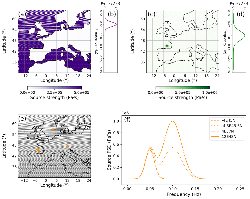
Figure 1Illustration of noise source model parametrization. The upper panels show spatial source distributions (a, c) with different spectra (b, d). Note the difference in maximum amplitudes. (Similar figures can be reproduced by following the Jupyter Notebook tutorial for noisi). Panel (e) shows the grid on which source spectra are defined; power spectral densities, corresponding to the term Snm of Eq. (4) for the grid locations ξ marked by yellow stars, are shown in (f). These are the superposition of spectra (b) and (d), with spatially varying amplitudes specified by distributions (a) and (c), respectively.
Since the rectangle rule is used for spatial integration (Eq. 7), a finer grid reduces integration error. For the comparison to SPECFEM3D_globe (shown below), the spacing is chosen as one half of the shortest expected seismic wave length, while for the synthetic inversion in Sect. 5.2, it is set to one quarter of the shortest wave length. Either rule of thumb produces satisfactory results, although small improvements are obtained using the finer spacing (see Supplement). To exclude that integration errors severely affect the modeled cross-correlations, testing the convergence of the results with decreasing grid step is recommended in particular when body waves in the cross-correlations are considered. Improvements of spatial integration are the subject of current developments (e.g., Igel, 2019).
The grid only defines source longitude and latitude but does not specify elevation. The influence of an eventual topography of the underlying wave propagation model on the surface area of each grid cell is neglected. However, topography itself can be taken into account; the Green's functions Gin describe propagation from and to the surface of the underlying numerical wave propagation model. Therefore, topography and bathymetry are determined by their value in the respective geographic location of the wave propagation model.
3.2 Source model parametrization
Instead of parametrizing the sources as fully sampled spectra at each grid point, their spectra are represented by a small number of Gaussian functions of frequency in each grid location, which reduces the dimensionality of the model and inverse problem and ensures that the source PSD in each location is smooth. This is illustrated in Fig. 1, which shows an example of a basic source model that may be subsequently updated by noise source inversion. The model contains sources which are homogeneously distributed throughout the ocean (panel a), as well as a localized source (panel c); note that their maximum amplitudes differ. Each of these distributions are associated with a different amplitude spectrum (panels b and d). Thus, in any location of the source grid, the effective source spectrum is a superposition of both spectra weighted by their respective distribution. This is shown in panel f, with spectra at locations marked by yellow stars on the map in panel e: On the continent (48∘ N, 12∘ E), the spectrum is flatly zero, whereas in the North Sea (57∘ N, 4∘ E) it shows a single peak associated with the source distribution and spectrum in panels a and b. In the Bay of Biscay, the localized strong source of panels c and d, which varies at shorter distance from 45∘ N, −4∘ E to 45.5∘ N, −4.5∘ E, is also visible.
Any number of such distributions can be superimposed to create a source model. Gaussian PSDs and their spatial weights at each grid point are stored in HDF5 format as detailed in the Appendix E. Examples for all input files are also provided in the GitHub repository. The parameters for setup are geographic distributions (geographically homogeneous, ocean, and Gaussian “blob”), as well as the central frequency and variance of the Gaussian spectra. Custom source models can be created by modifying the underlying HDF5 file (an example is shown in Sect. 5.1).
3.3 Wavefield databases
Green's functions are stored in one HDF5 file per seismic receiver component. The format is specified in the Appendix C. For the preparation of this
database, routines are provided that take a seismic station list, the format of which is also specified in the Appendix B, as input. One may set up a
database for analytic far-field surface wave Green's functions for 2-D homogeneous media (following Fan and Snieder, 2009); obtaining Green's functions
for PREM or other reference models additionally requires an instaseis database (e.g., downloaded from Syngine). If a surface wavefield output
from AxiSEM3D is provided, Green's functions can be extracted from this surface wavefield, allowing us to include 3-D lateral Earth structure. If run on
multiple processors, the task of preparing the Green's function database is performed in embarrassingly parallel mode in that each receiver component
is prepared on one core.
Custom wavefields can be built by converting the format of previously computed surface wavefields. Similarly to the example of converting from
AxiSEM3D output, output from any other wave propagation solver may be interpolated at the grid locations and stored in the HDF5 format as detailed in
the Appendix C for use with the noisi tool. Crucially, the HDF5 format (Folk et al., 2011) allows convenient access to single Green's functions. These
may be stored either as time series or complex spectra; details on this choice are explained below.
3.4 Evaluation of cross-correlations
The tool evaluates correlations for all possible combinations of stations specified in the station list (see Appendix B) and the selected component, optionally including auto-correlations. If run on multiple processors, tasks are again distributed according to a simple embarrassingly parallel scheme.
While the convolutions of Eqs. (4) and (6) are performed in the frequency domain for speed, storage of the Green's functions may be more convenient in the time or frequency domain depending on the application; procedures for either domain are implemented. When storage is in the frequency domain, no fast Fourier transform (FFT) of the Green's functions is needed during calculation, which eases the computation. As the Green's functions are real functions of time, their spectra are Hermitian so that storing their non-negative-frequency part suffices to describe them fully. However, the Green's functions have to be zero padded prior to fast Fourier transform in order to preclude circular convolution and to increase frequency resolution. When the Green's functions are stored in the time domain, this zero padding is done on the fly during computation before FFT is performed. Thus, the number of samples decreases compared to frequency domain storage, resulting in reduced storage and I/O effort despite the increased computational effort of performing FFT.
The resulting cross-correlations are saved in SAC format with essential metadata contained in the SAC header.
3.5 Measurements and evaluation of sensitivity kernels
To run noise source inversion, observed auto- and/or cross-correlations must be provided as SAC files with their headers containing a fixed set of metadata as specified in the Appendix A (usage similar to IRIS DMC, 2015). Measurements can then be performed on the data and the modeled cross-correlations yielding a misfit between the current model and the observations. Implemented measurements include windowed and full waveforms, mean squared amplitudes, and the logarithmic signal energy ratio between a causal and a-causal correlation branch. For details on these measurements, see Sager et al. (2018a). Running the measurement will additionally determine the term f(ω) of Eq. (6), which is frequently referred to as adjoint source. This term corresponds to the derivative of the measurement with respect to the synthetic cross-correlation trace. Sensitivity kernel computation is run analogous to the forward model, i.e., reading in Green's functions for each source location identified by index. Kernels are saved as ℓ by m by n dimensional arrays, where ℓ is the number of Gaussian PSD spectra, m the number of applied bandpass filters, and n the number of source locations.
To the best of our knowledge, the only currently available open-source model of noise cross-correlations and their sensitivity kernels was provided by
Tromp et al. (2010). Thus, we use their implementation to validate and cross-check the output of forward modeling with noisi. The
implementation by Tromp et al. (2010) follows a different strategy. It models the cross-correlation wavefield by inserting the inverse Fourier
transform of the term of Eq. (4) as a source term of the wave propagation simulation yielding in any location of the model domain.
To compare entirely independently computed ambient noise cross-correlations, we use AxiSEM3D (Leng et al., 2016) to create the pre-computed wavefields
on the basis of which we then compute cross-correlations with noisi. These are compared to cross-correlations modeled with SPECFEM3D_GLOBE
(Komatitsch and Tromp, 2002a, b) as described by Tromp et al. (2010) and in the SPECFEM3D_GLOBE user manual. To exclude relevant deviations
between the models stemming from differences between the spectral element solvers, we omit laterally varying crustal models since their
implementation differs between SPECFEM3D_GLOBE and AxiSEM3D and consider the elastic case without attenuation. We perform the comparison of
cross-correlations at periods of up to 15 s for the spherically symmetric PREM (Dziewoński and Anderson, 1981) and for the laterally varying S40RTS
(Ritsema et al., 2011) models. Using PREM, the effects of ocean, ellipticity, topography, rotation, and gravity were neglected, while they were included with
S40RTS. The ocean was modeled as an effective load in both solvers and gravity by the Cowling approximation (Komatitsch and Tromp, 2002a). Supplementary
Fig. S1 illustrates the locations of the stations in the modeling domain, which extends to 20∘ by 20∘, as well as the shear wave velocity
perturbation of S40RTS with respect to PREM in this region at 20 km depth. The numerical domain for the solution in SPECFEM3D_GLOBE is set to
40∘ by 40∘ with absorbing boundaries; the larger domain is chosen to exclude spurious boundary reflections of surface waves from the lag window
of interest. However, noise sources are restricted to act in the same domain as for the other case. In AxiSEM3D, a method that couples a
spectral-element discretization with a pseudospectral expansion along the azimuth (Leng et al., 2019), we simulate the full desired 3-D resolution
inside the domain of interest. Rather than using absorbing boundaries as in the simulation with SPECFEM3D_GLOBE, we avoid spurious reflections in
AxiSEM3D by using a global computational domain. The azimuthal Fourier expansion is tapered to a minimum of two Fourier coefficients outside of our
domain of interest, which strongly reduces the additional computing time accrued due to the global simulation.
As source distribution for this example, we chose a homogeneous distribution of noise with a Gaussian spectrum peaking at a 20 s
period. Figure 2 shows the comparison of cross-correlation waveforms obtained from SPECFEM3D_GLOBE and the combination of AxiSEM3D and
noisi interpolated to equal sampling rate and filtered consistently by a second-order Chebyshev low-pass filter. Each waveform is normalized
to unity for better visibility; a comparison showing the relative amplitudes can be found in the Supplement. The traces are arranged by increasing
inter-station distance (not to scale). We observe an excellent fit of the cross-correlation waveforms. Note that the strong asymmetry of several
cross-correlations is an effect of the sources being confined to a bounded domain, an effect which is reproduced consistently by both algorithms. This
figure also illustrates the effect of different models on the cross-correlations. The correlations for S40RTS show a delay in the arrival of the
dominant surface wave groups that increases with higher frequency, which is partially an effect of using different crustal layers (an averaged single
crustal layer was used with PREM), as well as the negative velocity perturbations of S40RTS from PREM in this region, which are illustrated in Fig. S1
in the Supplement.
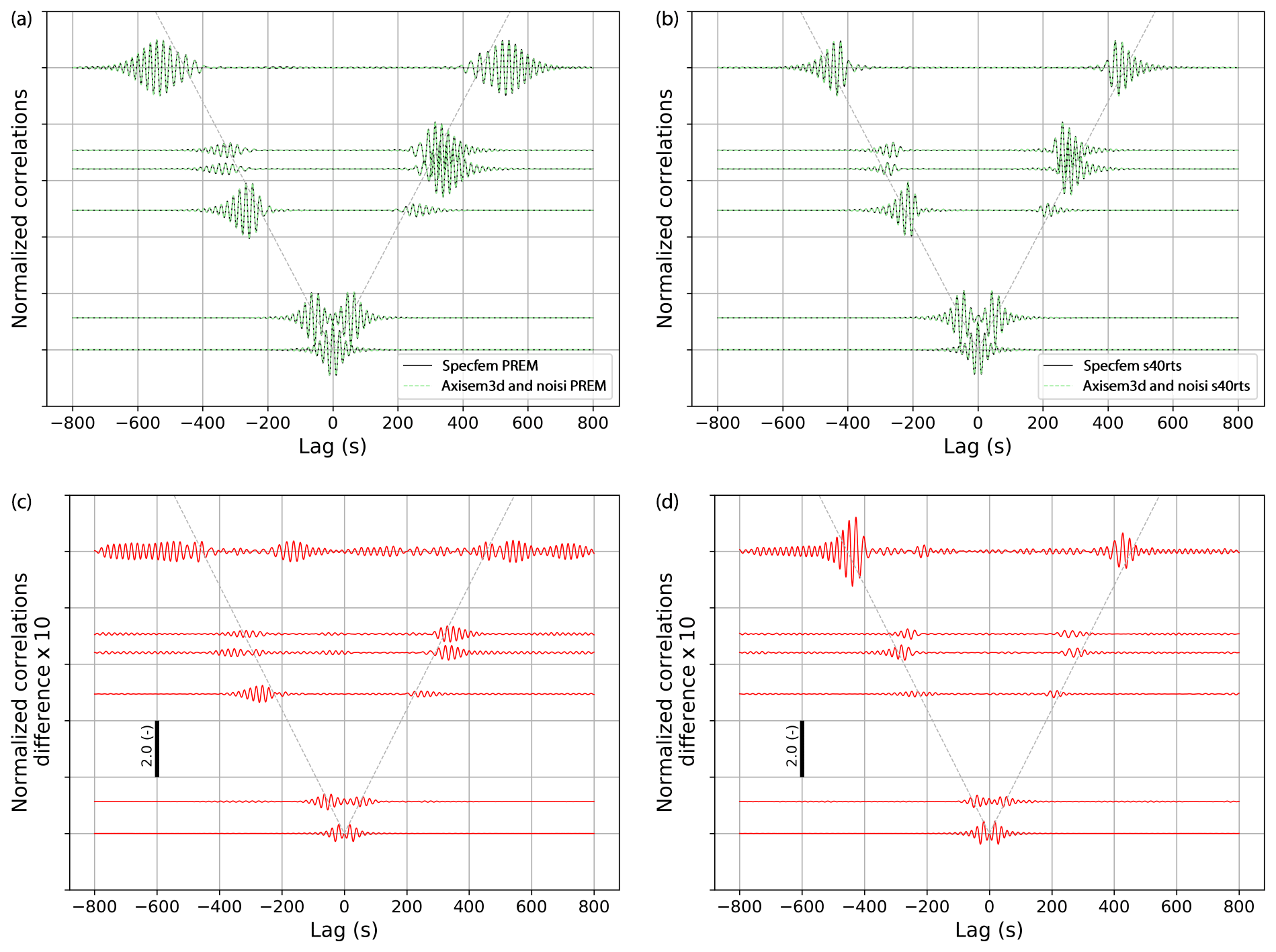
Figure 2Comparison between two implementations of simulation ambient noise cross-correlations with PREM (a) and S40RTS (b). Both panels shows correlations modeled with SPECFEM3D_GLOBE, as well as with noisi, in which the latter uses Green's functions modeled with AxiSEM3D. A moveout of 3 km s−1 is shown by the dashed gray line (note that the y axis is only approximately to scale for better visibility; however, the cross-correlations for both models are arranged at the same distances). The correlations are low-pass filtered by a type II Chebyshev filter with a stopband frequency of 0.07 Hz normalized to unity and arranged by inter-station distance. An overview of the modeling domain, stations, and mantle shear velocity model is shown in the Supplement. Panels (c) and (d) show the absolute difference between the traces in (a) and (b) enhanced by a factor of 10. The vertical bars denote the scale.
Upon close inspection, deviations of the correlations modeled by noisi from the SPECFEM3D_globe output are visible. Figure 2c and d show these increased by a factor of 10. We suggest that these result are mostly from the approximation of the spatial integral that we
adopt in Eq. (7). We corroborate this by varying the spatial sampling (see Supplement).
5.1 Auto- and cross-correlation forward modeling
Forward modeling of ambient noise auto- and cross-correlations has been employed in a number of studies, for example, to investigate noise sources
(e.g., Stutzmann et al., 2012; Gualtieri et al., 2013; Juretzek and Hadziioannou, 2017) or to evaluate the assumption of Green's function retrieval
(e.g., Stehly and Boué, 2017). The noisi tool implements forward modeling for arbitrary distributions of noise sources with Gaussian
spectra. To exemplify this, we model correlations of the Earth's hum at a selection of receiver locations based on the model of seismic hum as
described by Ardhuin et al. (2015) and implemented in Deen et al. (2018) and extended to global hum sources. We use a temporal subset of this space-,
time-, and frequency-dependent hum source model, namely a selection of Southern Hemisphere winter months (July–September) averaged over the frequency
band 0.0035–0.007 Hz. This hum model is interpolated on a dense global source grid for the noisi tool. To illustrate the use of
Green's functions describing different Earth structures and obtained with different wave propagation solvers, the correlations are constructed with
two different Green's function databases. Synthetics from anisotropic PREM with uniform crustal layer are contrasted with synthetics from S40RTS including attenuation, laterally varying crust2.0, and ocean load. These have been computed with AxiSEM3D (in spherically symmetric mode) and SPECFEM3D_GLOBE,
respectively.
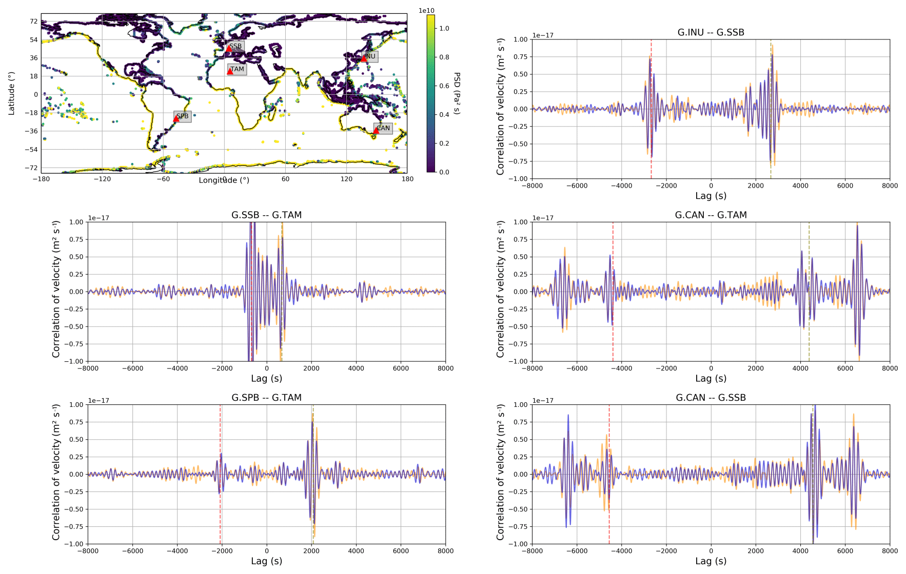
Figure 3Simulation of cross-correlations due to hum sources modeled akin to Ardhuin et al. (2015) and Deen et al. (2018). Hum sources are localized in small areas constrained to shorelines of continents and islands. Correlations were computed using both anisotropic PREM (yellow) and S40RTS (blue). Localized hum sources cause a host of early-arriving surface wave phases in the cross-correlations. Red and green vertical lines mark the arrival time of a surface wave traveling at 3.7 km s−1.
We illustrate a selection of the resulting correlations (selected to represent the variety of inter-station paths and distances) in Fig. 3. The map shows the averaged source model and station locations for the synthetic correlations. Additional panels show synthetic correlation traces for two Earth models (orange: PREM; blue: S40RTS+crust2.0). At the long periods considered here, the waveforms of both models are similar, although subtle differences occur both in phase and amplitude. Several cross-correlations show arrivals before the first-arriving Rayleigh wave (the arrival of a surface wave traveling at 3.7 km s−1 is marked by dashed red and green lines on the a-causal and causal branch, respectively). This occurs, for example, between stations CAN and SSB and stations INU and SSB. These phases, with amplitudes far higher than those expected of fast-traveling body waves, are due to the source distribution in this synthetic example; similar early-arriving phases have been previously observed. While sometimes referred to as spurious arrivals, they are physical and can even be utilized for source localization (Retailleau et al., 2017). Generally, the stationary phase of surface waves in the cross-correlation with respect to noise source distribution ensures the retrieval of fundamental mode surface waves from noise cross-correlations (Snieder, 2004; Tsai, 2009). However, the presence of strong or persistent localized sources off the great circle path which connects the two receivers can give rise to arrivals before the expected surface waves (e.g., Shapiro et al., 2006; Zheng et al., 2011), appearing approximately at the differential travel time from the source location to the two receivers. Modeling cross-correlations, such as the ones in Fig. 3, opens up possibilities to study them in more detail, which will possibly enable us to utilize valuable information which might otherwise be discarded as incoherent “noise”.
In a further step, we compare the model to observed cross-correlations. Since stacking duration was only 3 months for the noise source model (July–September 2013), only a few of the modeled station pairs yield cross-correlation with an acceptable signal-to-noise ratio. These are pairs of stations which are (i) exceptionally quiet in the hum band, according to probabilistic power spectral densities for the respective time period, and (ii) at moderate or near-antipodal distance to enhance station-to-station surface wave amplitude. These criteria are fulfilled by CAN, SSB, and TAM. We show a comparison of their observational cross-correlations with the modeled ones in Fig. 4. Cross-correlations were computed in windows of 12 h with 50 % overlap after removal of any earthquake with Mw>5.6 as classical, geometrically normalized cross-correlations according to Eq. (1) of Schimmel et al. (2011) and stacked. All waveforms in Fig. 4 are normalized by maximum amplitude.
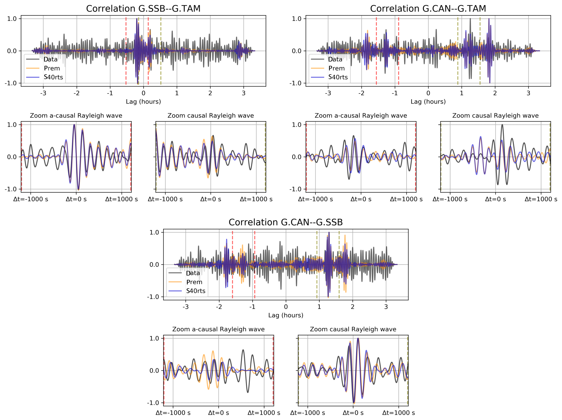
Figure 4Forward modeled and observed cross-correlations. No fitting or inversion was undertaken; the forward model is built upon the hum mechanism by Ardhuin et al. (2015) and Deen et al. (2018) using PREM (yellow lines) and S40RTS (blue lines). Correlations are normalized by maximum amplitude. Red and green vertical lines indicate windows of ± 20 min around a minor-arc surface wave traveling at 3.7 km s−1. These are enlarged in the respective bottom panels.
For better visibility, windows around the R1 wave are enlarged. Upon measuring the L2 waveform difference between observed and modeled cross-correlation within these windows, a slightly better overall fit is obtained by using a 3-D Earth model (this holds both for the three correlations selected here and the collection of all modeled correlations).
The observed cross-correlations are noisy due to the relatively short stack (up to 92 d depending on data availability); cross-correlations in this frequency band are expected to predominantly show direct, fundamental mode surface waves between two stations only after a stacking duration of one year and more (Haned et al., 2016). The observed traces here may contain incidental, non-coherent apparent correlations, i.e., “noise of the noise”, such as the strong arrival at Δt ≊ 500 s on the a-causal zoom of G.CAN–G.SSB. More elaborate stacking schemes (e.g., Schimmel et al., 2011; Ventosa et al., 2019), which are out of the scope of this work, can reduce such effects. It is important to note, however, that similar looking phases may also be produced by the inhomogeneous source distribution like the modeled arrival at Δt ≊ −300 s on the zoomed causal panel of G.CAN–G.TAM. Modeling can enable us to distinguish and interpret such phases.
5.2 Ambient noise source inversion
Sensitivity kernels computed with noisi can be used to run gradient-based inversion for the distribution of ambient seismic sources from a
dataset of observed ambient noise cross-correlations. To demonstrate the effectiveness of this approach, we conduct two synthetic inversions using
two different functions to measure the misfit between observations and model. The sensitivity kernel of any misfit function for the zz component of cross-correlation can be
expressed as
where merely the function fzz is determined by the chosen misfit function and corresponds to the derivative of the misfit function with respect to the modeled cross-correlation.
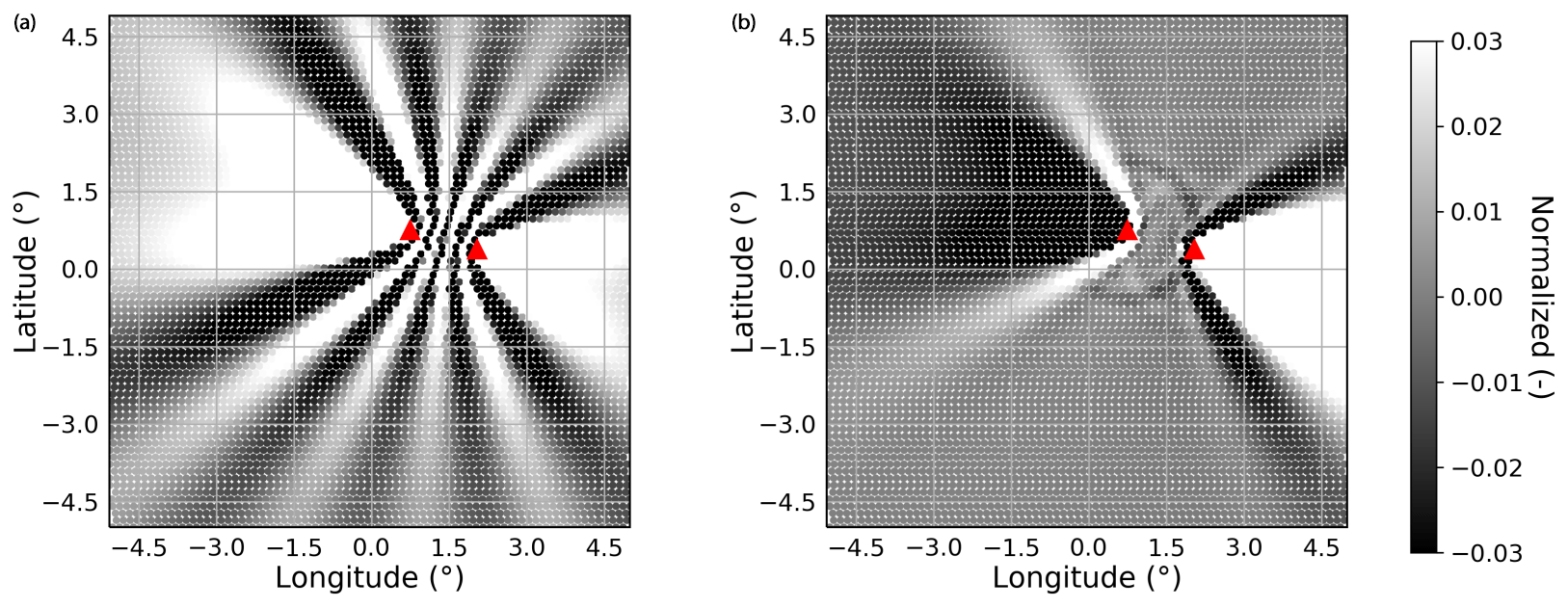
Figure 5Illustration of sensitivity kernels. (a) Normalized vertical-component sensitivity kernel of full waveform L2 misfit χfwi (Eq. 9). The station locations x1,x2 are marked by red triangles. Frequency integration runs from 0 Hz to the Nyquist frequency, but the source spectrum peaks at dominant frequency 0.05 Hz and filters out everything above 0.1 Hz. (b) Normalized sensitivity kernel of windowed asymmetry measurement χA (Eq. 11). Similar figures can be obtained by adapting the Jupyter Notebook tutorial for noisi.
As the first misfit function, we use the L2 norm of the synthetic (𝒞syn) and observed (𝒞obs) correlation waveforms, i.e.,
in the time domain, yielding
where we denote the Fourier transform by ℱ.
An exemplary waveform sensitivity kernel for the z components of both receivers and vertical sources is shown in Fig. 5a. It reveals how various locations of the source distribution affect the measurement. One can clearly recognize the pattern of stationary phase regions behind the stations and the oscillating sensitivity in between the stations (e.g., Snieder, 2004; Xu et al., 2019).
In contrast, Fig. 5b shows sensitivity Kzz of another misfit function,
where
and denote causal and a-causal windows of the cross-correlation, respectively, and f becomes the following (where the dependency on the lag τ is omitted):
For simplicity, we will refer to this second measurement as asymmetry in the following. This second sensitivity kernel (Fig. 5b) is smoother than the full waveform one; the oscillating sensitivity between the stations is removed due to the windowing by , and the stationary phase regions have opposite signs of sensitivity due to the ratio . A body wave is caught in the measurement window adding a faint ring of sensitivity near the stations probably due to body wave–surface wave interaction (Sager et al., 2018a). The term encompasses the differences between both sensitivity kernels of Fig. 5 by taking the form of Eqs. (10) and (13) for waveforms and asymmetry measurement, respectively.
This illustrates that inversions using different strategies to measure data-model misfits (waveform, asymmetry, etc.) will produce different optimal models of the noise source distribution. For example, provided adequate coverage, one can expect a higher resolution to result from using the L2 waveform misfit, which has more short-wavelength spatial features.
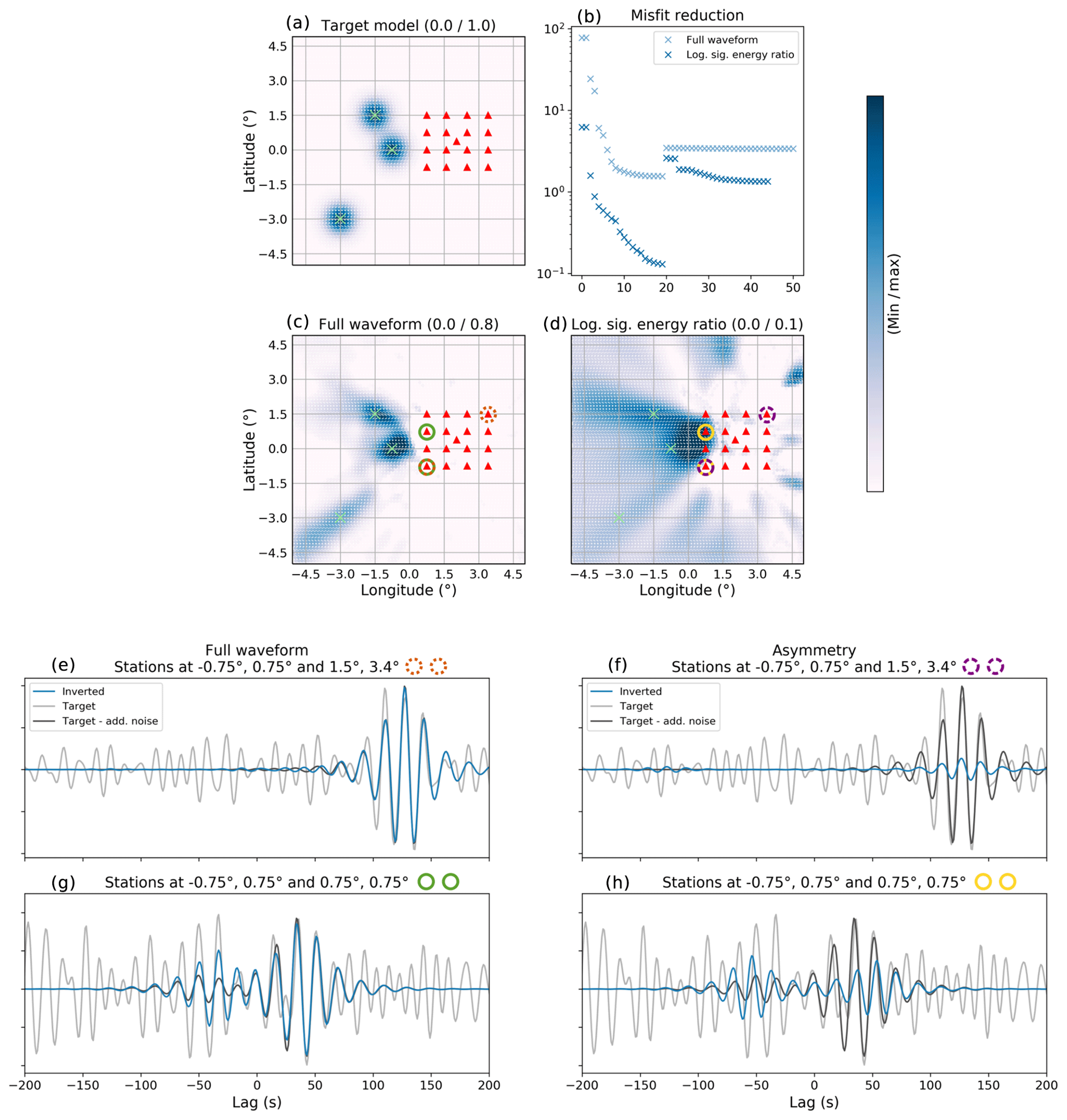
Figure 6(a, b) Synthetic inversions of ambient seismic source distribution. The target model is shown in (a). (b) shows the misfit reduction using two different measurements. After 20 iterations, an additional frequency band was added to the inversion, and smoothing decreased. (c, d) Recovered source distributions. Titles indicate the respective measurement; the numbers in brackets indicate the minimum and maximum values of the color scale. (e–h) Comparison of waveforms from the final models to the synthetic data. For this comparison, we chose a particularly good (e, f) and a particularly bad (g, h) example. Synthetic data from the target model, including additive noise, are shown by light gray lines. For comparison, we also show the noise-free synthetics in dark gray lines, which were not used for inversion but show that the inverted model retrieves the coherent information rather than the random noise. Modeled waveforms obtained from the inverted source distributions based on the full waveform and asymmetry are shown in blue. Colored circles indicate the location of the station pairs.
This appears even more clearly once we conduct the inversion. We first construct a synthetic dataset by forward modeling cross-correlations from a source distribution shown in Fig. 6a, which has a low background level of sources in the left half of the domain, along with three strong Gaussian-shaped sources marked by green crosses at varying distances outside the array, which is marked by red triangles. The right half of the domain is source free. The frequency content of the starting model is homogeneous for all sources (background and blobs), with Gaussian power spectral density S(ξ,ω) of Eq. (3) having a mean frequency of 0.05 Hz and standard deviation of 0.02 Hz. We compute cross-correlations through PREM at all station pairs of the array and add Gaussian noise with an amplitude of ± 5% of the average root mean square of all synthetic cross-correlation traces.
To treat the inversions with different measurements consistently, we proceed in the same manner concerning filtering and smoothing. The inversion starts at a lower frequency, and a higher frequency band is added (taking two measurements after bandpass filtering in two different bands) after 20 iterations. Gaussian smoothing is applied in lieu of a more formal regularization, and smoothing length is decreased after 20 iterations. The optimization itself is performed with the L-BFGS algorithm of the SciPy minimize module (Nocedal and Wright, 2006; Millman and Aivazis, 2011). Results are shown in Fig. 6. The second row (panels c and d) shows results from full waveform inversion (panel c) and asymmetry inversion (panel d). The centers of the Gaussian perturbations to be retrieved are marked by green crosses also on the recovered models to simplify comparison with the target model. Titles indicate the respective measurements, and numbers in brackets show the minimum and maximum of the recovered source distributions; the maximum amplitude of 1 is not fully recovered by any of the inversions due to the smoothing regularization.
As expected, the full waveform misfit performs better at recovering the perturbations. The recovery succeeds reasonably well for sources that are close to the array, whereas sources at a greater distance are more smeared both towards and away from the array. The sources close to the array suffer fairly little smoothing and demonstrate that it is possible to not only retrieve the direction but in this case also the approximate location of ambient noise sources predominantly imaged by fitting surface wave measurements.
The logarithmic signal energy ratio misfit shows stronger inversion artifacts and images a rather crude impression of the target model with stronger smearing effects. In addition, this inversion was terminated after 44 iterations due its falling below the threshold for minimal misfit improvement, which might indicate that it is trapped in a local minimum or simply suggests very slow convergence.
Figure 6e–h show example waveforms for two station pairs. Predicted waveforms by the final models (blue lines) are shown along with noise-free synthetic data (dark gray) and the synthetic data with additive noise which were used for inversion (light gray). Note that the gray traces do not vary between the left and right columns, whereas the blue traces show results for different measurements. Traces in the first row correspond to a station pair which is oriented southwest–northeast and marked by dashed circles, i.e., its stationary phase aligns approximately with the source at −3∘ and −3∘; the signal-to-noise-ratio is high, and the waveform measurement results in an excellent fit to the noise-free synthetic data. On the other hand, the bottom row corresponds to a station pair oriented north–south and marked by solid circles. In this case, sources in the stationary phase region are very low, and strong sources are located outside of it. The signal-to-noise ratio is low and the fit worse with some degree of overfitting. The asymmetry measurement appears to be more sensitive to additive noise and performs worse at recovering waveforms. For the favorably oriented station pair, it recovers phases reasonably well; amplitudes cannot be recovered with this measurement because it is based on a ratio that removes absolute amplitude information. For the unfavorably oriented station pair, neither phase nor amplitude fit well.
While the full waveform misfit produces a very satisfactory image in this synthetic case, it has a very low tolerance for errors in the seismic velocity
model (Sager et al., 2018b; Xu et al., 2019). On the other hand, the logarithmic energy ratio misfit, which produces a poor image of the target, is very robust
with respect to perturbations of the velocity model (Sager et al., 2018b) and has been shown to perform better in scenarios with spatially separated
source perturbations (Ermert et al., 2017; Sager et al., 2018b). Our proposed strategy for ambient seismic source inversion is to consider several misfits for
inversion and base interpretations on the synopsis of the results. The modular structure of noisi allows us to implement new measurement
functions without adapting any other part of the code by adding functions with the same call and return parameters to these scripts. Besides the
measurements illustrated above, the L2 misfit of signal energy in the surface wave window is implemented.
The noisi tool allows users to create correlations for a variety of source models without the burden of costly numerical wave propagation
simulations by utilizing instaseis or to run noise source inversion at reduced cost with pre-calculated Green's function databases from
AxiSEM3D or other wave propagation solvers. Due to its implementation in Python, the tool can be easily modified and integrated into a rapidly growing
ecosystem of seismologic applications in Python (e.g., Beyreuther et al., 2010; Hosseini and Sigloch, 2017; van Driel et al., 2015; Heimann et al., 2019; Lecocq et al., 2014).
Disadvantages compared to implementations integrated into spectral element solvers, such as the ones by Tromp et al. (2010) and Sager et al. (2018a), are
the rigid setting of the source grid and the approximation of spatial integrals. These are evaluated by weighted sums which can lead to
approximation artifacts (see Fig. 2). Tromp et al. (2010), Basini et al. (2013), and Sager et al. (2018a) evaluate the spatial integrals using the
spectral element basis, which is expected to approximate the integral better at a comparable spatial resolution. However, this is not a conceptual but
rather a current practical limitation of the tool and could thus be overcome by adapting the wavefield storage and spatial integration. While the
errors in Fig. 2c and d may appear large, they may often be negligible in comparison to data noise and can be further diminished
by increased spatial sampling. The storage burden of the Green's function database may be regarded as another disadvantage. However, wavefields at the
surface of the modeling domain have to be temporarily stored in either type of implementation to allow the application of the ambient source spectra,
and thus the choice to reuse them appears intuitive. Finally, and most importantly, the tool is not fit to perform ambient noise full waveform
adjoint tomography. This task requires iterative updates to the Earth model and can be achieved by SPECFEM3D_globe or the recently developed Salvus
(Afanasiev et al., 2018). Both of these implement a spectral element model of the cross-correlation wavefield (Tromp et al., 2010; Sager et al., 2020). Extension of
noisi to compute structure sensitivity kernels is possible but highly impractical because storing the required volume wavefield would be
cumbersome, and the re-computation of the wavefield after each structural update would defeat the purpose of using pre-computed wavefields.
The output of the wavefield at the Earth's surface either in full or sampled at particular predefined grid locations poses practical challenges for
input/output and storage in both types of applications. As an example, the retained wavefield utilized by SPECFEM3D_GLOBE for creating the
cross-correlations of a single reference station in Fig. 2 amounts to 180 GB for the 40∘ by 40∘ domain with 15 s being the shortest period. Furthermore, the wavefield at the surface needs to be either post-processed for usage with noisi or convolved with the
ambient noise source spectrum (e.g., Tromp et al., 2010). This is made cumbersome by the high temporal sampling of the numerical wavefield, which is
imposed by the Courant–Friedrichs–Lewy criterion. The ease of computing cross-correlations with noisi is in part a consequence of decimating simulated Green's
functions in time by factors of 10 and more. In turn, built-in sparser representation and/or output of the surface wavefield in numerical solvers,
such as currently implemented by Salvus (Boehm et al., 2016), partially alleviates the burden and may pave the way for faster and computationally cheaper
noise cross-correlation modeling without recourse to pre-calculated wavefields. In the meantime, further developments of the presented tool may
include improvements of the spatial integration. To the best of our knowledge, it closes a current gap in the application of Green's function
databases for noise cross-correlation modeling.
The following SAC headers on observed cross-correlation traces can be used with noisi in order to perform measurements with the goal of
ambient seismic source inversion. Only a few of them are essential to provide the necessary information to the tool. These are marked in bold.
| b: (float), minimum lag |
| e: (float), maximum lag |
| stla: (float), latitude of station 1 |
| stlo: (float), longitude of station 1 |
| evla: (float), latitude of station 2 |
| evlo: (float), longitude of station 2 |
| user0: (float), number of stacked windows |
| user1: (float), window length for observed cross-correlation computation |
| user2: (float), window overlap during observed cross-correlation computation |
| dist: (float), station pair distance in meters |
| az: (float), station pair azimuth in degrees |
| baz: (float), station pair back azimuth in degrees |
| kstnm: (string), station code of station 1 |
| kevnm: (string), station code of station 1 |
| kt0: (string), date of earliest window in cross-correlation stack (YYYYjjj) |
| kt1: (string), date of latest window in cross-correlation stack (YYYYjjj) |
| kuser0: (string), network code of station 2 |
| kuser1: (string), location code of station 2 |
| kuser2: (string), channel code of station 2 |
| kcmpnm: (string), channel code of station 1 |
| knetwk: (string), network code of station 1 |
Stations to be used in modeling need to be specified in a comma-separated list (with one example line) as follows.
| net,sta,lat,lon |
| G,CAN,-35.318715,148.996325 |
The tool expects to find Green's functions organized as HDF5 files by seismic receiver channel with filenames NETWORK.STATION..CHANNEL.h5 for the
networks and stations listed in the input file list (see above). Each HDF5 file needs to contain the following data structure. Both single and double
precision floats may be used for the “data” and “sourcegrid” datasets. Single precision is used by default.
| group “/” | ||
| dataset ”data” (float), shape: ntraces by nt, Green's functions | ||
| dataset “sourcegrid” (float), shape: 2 by ntraces, geographic grid | ||
| dataset “stats”, metadata | attribute ”Fs” (float), sampling rate in Hz | |
| attribute “data_quantity” (string), ”DIS”, ”VEL” or ”ACC” | ||
| attribute “fdomain” (int), 0 for time domain, 1 for frequency domain | ||
| attribute “nt” (int), number of samples | ||
| attribute “ntraces” (int), number of source locations | ||
| attribute reference_station (string), SEED identifier of station |
The tool expects to find the noise source model as HDF5 files with name starting_model.h5 (for each iteration) with the following data structure.
| group “/” | |
| dataset “coordinates” (float), shape: 2 by ntraces; geographic grid | |
| dataset “frequencies” (float), shape: Number of frequency samples after zero-padded, next power of 2, real FFT of nt; frequency axis | |
| dataset “model” (float), shape: ntraces by number of basis functions; spatial weights of noise source model | |
| dataset “spectral_basis” (float), shape: number of basis functions by length of frequency axis; spectral basis functions | |
| dataset “surface_areas” (float), shape: ntraces; approximate surface area of grid cell |
The Python code can be downloaded from GitHub (https://github.com/lermert/noisi, Ermert and Igel, 2020). A tutorial in the form of a Jupyter Notebook is provided as the main item of documentation and details each step for the computation of cross-correlations and sensitivity kernels.
The GitHub repository contains a set of basic test cases to be passed by further developments. It also provides a numerical test for the consistency of forward model and gradient, which can be employed for the development of additional misfit functions.
All observed seismic data used to prepare this paper were downloaded from IRIS Data Management Center.
The supplement related to this article is available online at: https://doi.org/10.5194/se-11-1597-2020-supplement.
LE implemented the current version of noisi and ran the comparison with specfem, the forward model, and the synthetic
inversions. KS and JI continuously contributed suggestions for the conceptual setup and improvement of the tool. KS provided advice on the
inversion, and JI intensively test-ran the code in the course of further developments. ES computed the global hum source input model and reviewed
the observational and synthetic cross-correlation results. ES, TNM, and AF provided scientific advice. A first version of the paper was drafted
by LE and continuously improved upon by discussions with and suggestions from all authors.
The authors declare that they have no conflict of interest.
The authors thank Kees Wapenaar and Erdinc Saygin for their thoughtful, constructive reviews on the paper, and the topical and executive editors of Solid Earth, Michal Malinowski and Charlotte Krawczyk, for its efficient handling. Laura Ermert gratefully acknowledges support from the Swiss National Science Foundation under grant P2EZP2_175124 and thanks Naiara Korta Martiartu for improvement suggestions to the paper. A warm thank you also to Kuangdai Leng for valuable help with AxiSEM3D. Korbinian Sager thanks the Swiss National Science Foundation for support under grant P2EZP2_184379. Computations were run on the UK national supercomputer ARCHER under Laura Ermert's driving test allocation and Tarje Nissen-Meyer's NERC remit. Observational data were obtained from the IRIS Data Management Center. IRIS Data Services are funded through the Seismological Facilities for the Advancement of Geoscience and EarthScope (SAGE) proposal of the National Science Foundation under Cooperative Agreement EAR-1261681.
This research has been supported by the Swiss National Science Foundation (grant no. 175124, http://p3.snf.ch/project-175124, last access: 26 August 2020, and grant no. 184379, http://p3.snf.ch/project-184379, last access: 26 August 2020).
This paper was edited by Michal Malinowski and reviewed by Erdinc Saygin and Cornelis Wapenaar.
Afanasiev, M., Boehm, C., van Driel, M., Krischer, L., Rietmann, M., May, D. A., Knepley, M. G., and Fichtner, A.: Modular and flexible spectral-element waveform modelling in two and three dimensions, Geophys. J. Int., 216, 1675–1692, https://doi.org/10.1093/gji/ggy469, 2018. a
Aki, K.: Space and time spectra of stationary stochastic waves, with special reference to microtremors, B. Earthq. Res. I. Tokyo, 35, 415–456, 1957. a
Aki, K. and Richards, P.: Quantitative Seismology, University Science Books, Mill Valley, California, 2002. a, b
Ardhuin, F., Stutzmann, E., Schimmel, M., and Mangeney, A.: Ocean wave sources of seismic noise, J. Geophys. Res., 116, C09004, https://doi.org/10.1029/2011JC006952, 2011. a
Ardhuin, F., Gualtieri, L., and Stutzmann, E.: How ocean waves rock the Earth: Two mechanisms explain microseisms with periods 3 to 300 s, Geophys. Res. Lett., 42, 765–772, https://doi.org/10.1002/2014GL062782, 2015. a, b, c
Bard, P.-Y., Cadet, H., Endrun, B., Hobiger, M., Renalier, F., Theodulidis, N., Ohrnberger, M., Fäh, D., Sabetta, F., Teves-Costa, P., Duval, A.-M., Cornou, C., Guillier, B., Wathelet, M., Savvaidis, A., Köhler, A., Burjanek, J., Poggi, V., Gassner-Stamm, G., Havenith, H., Hailemikael, S., Almeida, J., Rodrigues, I., Veludo, I., Lacave, C., Thomassin, S., and Kristekova, M.: From Non-invasive Site Characterization to Site Amplification: Recent Advances in the Use of Ambient Vibration Measurements, Springer, Dordrecht, 2010. a
Basini, P., Nissen-Meyer, T., Boschi, L., Casarotti, E., Verbeke, J., Schenk, O., and Giardini, D.: The influence of nonuniform ambient noise on crustal tomography in Europe, Geochem. Geoph. Geosy., 14, 1471–1492, 2013. a, b
Beyreuther, M., Barsch, R., Krischer, L., Megies, T., Behr, Y., and Wassermann, J.: ObsPy: A Python Toolbox for Seismology, Seismol. Res. Lett., 81, 530–533, https://doi.org/10.1785/gssrl.81.3.530, 2010. a, b
Boehm, C., Hanzich, M., de la Puente, J., and Fichtner, A.: Wavefield compression or adjoint methods in full-waveform inversion, Geophysics, 81, R385–R397, 2016. a
Bowden, D. C., Tsai, V. C., and Lin, F. C.: Site amplification, attenuation, and scattering from noise correlation amplitudes across a dense array in Long Beach, CA, Geophys. Res. Lett., 42, 1360–1367, https://doi.org/10.1002/2014GL062662, 2015. a
Brenguier, F., Shapiro, N. M., Campillo, M., Ferrazzini, V., Duputel, Z., Coutant, O., and Nercessian, A.: Towards forecasting volcanic eruptions using seismic noise, Nat. Geosci., 1, 126–130, 2008. a
Claerbout, J.: Synthesis of a layered medium from its acoustic transmission response, Geophysics, 33, 264–269, 1968. a
Clements, T. and Denolle, M. A.: Tracking Groundwater Levels Using the Ambient Seismic Field, Geophys. Res. Lett., 45, 6459–6465, https://doi.org/10.1029/2018GL077706, 2018. a
Collette, A.: Python and HDF5, O'Reilly, Sebastopol, California, 2013. a
Cupillard, P. and Capdeville, Y.: On the amplitude of surface waves obtained by noise correlation and the capability to recover the attenuation: a numerical approach, Geophys. J. Int., 181, 1687–1700, 2010. a
Dahm, T., Heimann, S., Funke, S., Wendt, S., Rappsilber, I., Bindi, D., Plenefisch, T., and Cotton, F.: Seismicity in the block mountains between Halle and Leipzig, Central Germany: centroid moment tensors, ground motion simulation, and felt intensities of two M∼3 earthquakes in 2015 and 2017, J. Seismol., 22, 985–1003, 2018. a
Dalcín, L., Paz, R., and Storti, M.: MPI for Python, J. Parallel Distr. Com., 65, 1108–1115, 2005. a, b
Datta, A., Hanasoge, S., and Goudswaard, J.: Finite-Frequency Inversion of Cross-Correlation Amplitudes for Ambient Noise Source Directivity Estimation, J. Geophys. Res., 124, 6653–6665, https://doi.org/10.1029/2019JB017602, 2019. a, b, c, d
Deen, M., Stutzmann, E., and Ardhuin, F.: The Earth's Hum Variations From a Global Model and Seismic Recordings Around the Indian Ocean, Geochem. Geoph. Geosy., 19, 4006–4020, https://doi.org/10.1029/2018GC007478, 2018. a, b, c
Delaney, E., Ermert, L., Sager, K., Kritski, A., Bussat, S., and Fichtner, A.: Removal of traveltime errors in time-lapse passive seismic monitoring induced by non-stationary noise sources, Geophysics, 82, KS57–KS70, 2017. a
Denolle, M. A., Dunham, E. M., Prieto, G. A., and Beroza, G. C.: Ground motion prediction of realistic earthquake sources using the ambient seismic field, J. Geophys. Res., 118, 2102–2118, https://doi.org/10.1029/2012JB009603, 2013. a
de Ridder, S. A. L., Biondi, B. L., and Clapp, R. G.: Time-lapse seismic noise correlation tomography at Valhall, Geophys. Res. Lett., 41, 6116–6122, https://doi.org/10.1002/2014GL061156, 2014. a
Dziewoński, A. M. and Anderson, D. L.: Preliminary reference Earth model, Phys. Earth Planet. In., 25, 297–356, 1981. a, b
Ermert, L. and Igel, J.: noisi, GitHub, available at: https://github.com/lermert/noisi, last access: 26 August 2020. a
Ermert, L., Sager, K., Afanasiev, M., Boehm, C., and Fichtner, A.: Ambient seismic source inversion in a heterogeneous Earth – Theory and application to the Earth's hum, J. Geophys. Res., 122, 9184–9207, https://doi.org/10.1002/2017JB014738, 2017. a, b, c, d, e
Fan, Y. and Snieder, R.: Required source distribution for interferometry of waves and diffusive fields, Geophys. J. Int., 179, 1232–1244, https://doi.org/10.1111/j.1365-246X.2009.04358.x, 2009. a, b, c
Fang, H., Yao, H., Zhang, H., Huang, Y.-C., and van der Hilst, R. D.: Direct inversion of surface wave dispersion for three-dimensional shallow crustal structure based on ray tracing: methodology and application, Geophys. J. Int., 201, 1251, https://doi.org/10.1093/gji/ggv080, 2015. a
Farra, V., Stutzmann, E., Gualtieri, L., Schimmel, M., and Ardhuin, F.: Ray-theoretical modeling of secondary microseism P waves, Geophys. J. Int., 206, 1730, https://doi.org/10.1093/gji/ggw242, 2016. a
Fichtner, A.: Source and processing effects on noise correlations, Geophys. J. Int., 197, 1527–1531, 2014. a, b, c, d
Fichtner, A. and Simutė, S.: Hamiltonian Monte Carlo Inversion of Seismic Sources in Complex Media, J. Geophys. Res., 123, 2984–2999, https://doi.org/10.1002/2017JB015249, 2018. a
Folk, M., Heber, G., Koziol, Q., Pourmal, E., and Robinson, D.: An overview of the HDF5 technology suite and its applications, in: Proceedings of the EDBT/ICDT 2011 Workshop on Array Databases, Uppsala, Sweden, March 2011, 36–47, ACM, 2011. a, b
Gualtieri, L. and Ekström, G.: Broad-band seismic analysis and modeling of the 2015 Taan Fjord, Alaska landslide using Instaseis, Geophys. J. Int., 213, 1912–1923, 2018. a
Gualtieri, L., Stutzmann, E., Capdeville, Y., Ardhuin, F., Schimmel, M., Mangeney, A., and Morelli, A.: Modelling secondary microseismic noise by normal mode summation, Geophys. J. Int., 193, 1732–1745, 2013. a
Halliday, D. and Curtis, A.: Seismic interferometry, surface waves and source distribution, Geophys. J. Int., 175, 1067–1087, https://doi.org/10.1111/j.1365-246X.2008.03918.x, 2008. a, b, c
Hanasoge, S. M.: The influence of noise sources on cross-correlation amplitudes, Geophys. J. Int., 192, 295–309, https://doi.org/10.1093/gji/ggs015, 2013a. a, b, c
Hanasoge, S. M.: Measurements and kernels for source-structure inversions in noise tomography, Geophys. J. Int., 196, 971–985, https://doi.org/10.1093/gji/ggt411, 2013b. a
Haned, A., Stutzmann, E., Schimmel, M., Kiselev, S., Davaille, A., and Yelles-Chaouche, A.: Global tomography using seismic hum, Geophys. J. Int., 204, 1222, https://doi.org/10.1093/gji/ggv516, 2016. a, b
Heimann, S., Vasyura-Bathke, H., Sudhaus, H., Isken, M. P., Kriegerowski, M., Steinberg, A., and Dahm, T.: A Python framework for efficient use of pre-computed Green's functions in seismological and other physical forward and inverse source problems, Solid Earth, 10, 1921–1935, https://doi.org/10.5194/se-10-1921-2019, 2019. a, b
Hosseini, K. and Sigloch, K.: ObspyDMT: a Python toolbox for retrieving and processing large seismological data sets, Solid Earth, 8, 1047–1070, https://doi.org/10.5194/se-8-1047-2017, 2017. a
Igel, J.: Near Real-Time Finite-Frequency Ambient Seismic Noise Source Inversion, Masterarbeit ETH Zürich, 2019. a
IRIS: The IRIS Synthetics Engine, Incorporated Research Institutions for Seismology, Washington, DC, https://doi.org/10.17611/DP/SYNGINE.1, 2015. a
Juretzek, C. and Hadziioannou, C.: Linking source region and ocean wave parameters with the observed primary microseismic noise, Geophys. J. Int., 211, 1640–1654, https://doi.org/10.1093/gji/ggx388, 2017. a
Kimman, W. and Trampert, J.: Approximations in seismic interferometry and their effects on surface waves, Geophys. J. Int., 182, 461–476, 2010. a, b, c
Komatitsch, D. and Tromp, J.: Spectral-element simulations of global seismic wave propagation, Part II: 3-D models, oceans, rotation, and gravity, Geophys. J. Int., 150, 303–318, 2002a. a, b
Komatitsch, D. and Tromp, J.: Spectral-element simulations of global seismic wave propagation, Part I: validation, Geophys. J. Int., 149, 390–412, 2002b. a
Krischer, L., Hutko, A. R., Van Driel, M., Stähler, S., Bahavar, M., Trabant, C., and Nissen-Meyer, T.: On-demand custom broadband synthetic seismograms, Seismol. Res. Lett., 88, 1127–1140, 2017. a, b, c
Laske, G., Masters., G., Ma, Z. and Pasyanos, M.: Update on CRUST1.0 – A 1-degree Global Model of Earth's Crust, Geophys. Res. Abstr., EGU2013-2658, EGU General Assembly 2013, Vienna, Austria, 2013. a
Lecocq, T., Caudron, C., and Brenguier, F.: MSNoise, a Python Package for Monitoring Seismic Velocity Changes Using Ambient Seismic Noise, Seismol. Res. Lett., 85, 715–726, https://doi.org/10.1785/0220130073, 2014. a, b
Leng, K., Nissen-Meyer, T., and van Driel, M.: Efficient global wave propagation adapted to 3-D structural complexity: a pseudospectral/spectral-element approach, Geophys. J. Int., 207, 1700, https://doi.org/10.1093/gji/ggw363, 2016. a, b
Leng, K., Nissen-Meyer, T., van Driel, M., Hosseini, K., and Al-Attar, D.: AxiSEM3D: broad-band seismic wavefields in 3-D global earth models with undulating discontinuities, Geophys. J. Int., 217, 2125–2146, https://doi.org/10.1093/gji/ggz092, 2019. a, b
IRIS DMC: Data Services Products: Global Empirical Greens Tensors, Incorporated Research Institutions for Seismology, Washington, DC, https://doi.org/10.17611/DP/GEGT.1, 2015. a
Millman, K. J. and Aivazis, M.: Python for Scientists and Engineers, Comput. Sci. Eng., 13, 9–12, https://doi.org/10.1109/MCSE.2011.36, 2011. a, b
Nakata, N., Gualtieri, L., and Fichtner, A.: Seismic Ambient Noise, Cambridge University Press, Cambridge, New York, 2019. a
Nie, S., Anthony, D., and Ma, S.: Testing the Amplitude of the Deconvolution-Based Ambient-Field Green's Functions by 3-D Simulations of Elastic Wave Propagation in Sedimentary Basins, J. Geophys. Res.-Sol. Ea., 124, 7213–7226, https://doi.org/10.1029/2018JB017197, 2019. a
Nishida, K. and Fukao, Y.: Source distribution of Earth's background free oscillations, J. Geophys. Res., 112, b06306, https://doi.org/10.1029/2006JB004720, 2007. a, b, c
Nishida, K. and Takagi, R.: Teleseismic S wave microseisms, Science, 353, 919–921, 2016. a
Nishida, K., Montagner, J.-P., and Kawakatsu, H.: Global Surface Wave Tomography Using Seismic Hum, Science, 326, 112–112, https://doi.org/10.1126/science.1176389, 2009. a
Nocedal, J. and Wright, S. J.: Large-scale unconstrained optimization, in: Numerical Optimization, Springer, New York, 164–192, 2006. a
Obermann, A., Planès, T., Larose, E., and Campillo, M.: Imaging preeruptive and coeruptive structural and mechanical changes of a volcano with ambient seismic noise, J. Geophys. Res., 118, 6285–6294, https://doi.org/10.1002/2013JB010399, 2013. a
Oliphant, T. E.: A guide to NumPy, Vol. 1, available at: http://web.mit.edu/dvp/Public/numpybook.pdf, last access: 26 August 2020. a
Retailleau, L., Boué, P., Stehly, L., and Campillo, M.: Locating Microseism Sources Using Spurious Arrivals in Intercontinental Noise Correlations, J. Geophys. Res., 122, 8107–8120, https://doi.org/10.1002/2017JB014593, 2017. a
Retailleau, L., Landès, M., Gualtieri, L., Shapiro, N. M., Campillo, M., Roux, P., and Guilbert, J.: Detection and analysis of a transient energy burst with beamforming of multiple teleseismic phases, Geophys. J. Int., 212, 14–24, https://doi.org/10.1093/gji/ggx410, 2018. a
Ritsema, J., Deuss, A., van Heijst, H. J., and Woodhouse, J. H.: S40RTS: a degree-40 shear-velocity model for the mantle from new Rayleigh wave dispersion, teleseismic traveltime and normal-mode splitting function measurements, Geophys. J. Int., 184, 1223–1236, 2011. a
Romero, P. and Schimmel, M.: Mapping the basement of the Ebro Basin in Spain with seismic ambient noise autocorrelations, J. Geophys. Res., 123, 5052–5067, 2018. a
Roten, D., Fäh, D., Cornou, C., and Giardini, D.: Two-dimensional resonances in Alpine valleys identified from ambient vibration wavefields, Geophys. J. Int., 165, 889–905, 2006. a
Sadeghisorkhani, H., Gudmundsson, O., Roberts, R., and Tryggvason, A.: Velocity-measurement bias of the ambient noise method due to source directivity: a case study for the Swedish National Seismic Network, Geophys. J. Int., 209, 1648, https://doi.org/10.1093/gji/ggx115, 2017. a
Sager, K., Boehm, C., Ermert, L., Krischer, L., and Fichtner, A.: Sensitivity of Seismic Noise Correlation Functions to Global Noise Sources, J. Geophys. Res., 123, 6911–6921, https://doi.org/10.1029/2018JB016042, 2018a. a, b, c, d, e
Sager, K., Ermert, L., Boehm, C., and Fichtner, A.: Towards full waveform ambient noise inversion, Geophys. J. Int., 212, 566–590, https://doi.org/10.1093/gji/ggx429, 2018b. a, b, c, d, e
Sager, K., Boehm, C., Ermert, L., Krischer, L., and Fichtner, A.: Global-Scale Full-Waveform Ambient Noise Inversion, J. Geophys. Res., 125, e2019JB018644, https://doi.org/10.1029/2019JB018644, 2020. a, b, c, d
Sánchez-Pastor, P., Obermann, A., Schimmel, M., Weemstra, C., Verdel, A., and Jousset, P.: Short- and Long-Term Variations in the Reykjanes Geothermal Reservoir From Seismic Noise Interferometry, Geophys. Res. Lett., 46, 5788–5798, https://doi.org/10.1029/2019GL082352, 2019. a
Saygin, E., Cummins, P. R., and Lumley, D.: Retrieval of the P wave reflectivity response from autocorrelation of seismic noise: Jakarta Basin, Indonesia, Geophys. Res. Lett., 44, 792–799, 2017. a
Schimmel, M., Stutzmann, E., and Gallart, J.: Using instantaneous phase coherence for signal extraction from ambient noise data at a local to a global scale, Geophys. J. Int., 184, 494–506, 2011. a, b
Sens-Schönfelder, C. and Wegler, U.: Passive image interferometry and seasonal variations of seismic velocities at Merapi Volcano, Indonesia, Geophys. Res. Lett., 33, l21302, https://doi.org/10.1029/2006GL027797, 2006. a
Shapiro, N. M. and Campillo, M.: Emergence of broadband Rayleigh waves from correlations of the ambient seismic noise, Geophys. Res. Lett., 31, l07614, https://doi.org/10.1029/2004GL019491, 2004. a
Shapiro, N. M., Campillo, M., Stehly, L., and Ritzwoller, M.: High resolution surface wave tomography from ambient seismic noise, Science, 307, 1615–1618, 2005. a
Shapiro, N. M., Ritzwoller, M., and Bensen, G.: Source location of the 26 sec microseism from cross-correlations of ambient seismic noise, Geophys. Res. Lett., 33, L18310, https://doi.org/10.1029/2006GL027010, 2006. a
Simonov, K.: PyYAML, available at: https://pypi.org/project/PyYAML/ (last access: 26 August 2020), 2014. a
Singer, J., Obermann, A., Kissling, E., Fang, H., Hetényi, G., and Grujic, D.: Along-strike variations in the Himalayan orogenic wedge structure in Bhutan from ambient seismic noise tomography, Geochem. Geoph. Geosy., 18, 1483–1498, 2017. a
Snieder, R.: Extracting the Green's function from the correlation of coda waves: A derivation based on stationary phase, Phys. Rev. E, 69, 046610, https://doi.org/10.1103/PhysRevE.69.046610, 2004. a, b, c
Stehly, L. and Boué, P.: On the interpretation of the amplitude decay of noise correlations computed along a line of receivers, Geophys. J. Int., 209, 358, https://doi.org/10.1093/gji/ggx021, 2017. a, b, c
Stehly, L., Campillo, M., and Shapiro, N. M.: A study of the seismic noise from its long-range correlation properties, J. Geophys. Res., 111, B10306, https://doi.org/10.1029/2005JB004237, 2006. a
Stehly, L., Campillo, M., Froment, B., and Weaver, R. L.: Reconstructing Green's function by correlation of the coda of the correlation (C3) of ambient seismic noise, J. Geophys. Res., 113, b11306, https://doi.org/10.1029/2008JB005693, 2008. a
Stehly, L., Fry, B., Campillo, M., Shapiro, N., Guilbert, J., Boschi, L., and Giardini, D.: Tomography of the Alpine region from observations of seismic ambient noise, Geophys. J. Int., 178, 338–350, 2009. a
Stutzmann, E., Ardhuin, F., Schimmel, M., Mangeney, A., and Patau, G.: Modelling long-term seismic noise in various environments, Geophys. J. Int., 191, 707–722, https://doi.org/10.1111/j.1365-246X.2012.05638.x, 2012. a, b, c
Taylor, G., Rost, S., and Houseman, G.: Crustal imaging across the North Anatolian Fault Zone from the autocorrelation of ambient seismic noise, Geophys. Res. Lett., 43, 2502–2509, 2016. a
Tromp, J., Luo, Y., Hanasoge, S., and Peter, D.: Noise cross-correlation sensitivity kernels, Geophys. J. Int., 183, 791–819, 2010. a, b, c, d, e, f, g, h, i, j, k, l
Tsai, V. C.: On establishing the accuracy of noise tomography traveltime measurements in a realistic medium, Geophys. J. Int., 178, 1555–1564, 2009. a
van Driel, M., Krischer, L., Stähler, S. C., Hosseini, K., and Nissen-Meyer, T.: Instaseis: instant global seismograms based on a broadband waveform database, Solid Earth, 6, 701–717, https://doi.org/10.5194/se-6-701-2015, 2015. a, b, c, d
Ventosa, S., Schimmel, M., and Stutzmann, E.: Towards the Processing of Large Data Volumes with Phase Cross-Correlation, Seismol. Res. Lett., 90, 1663–1669, https://doi.org/10.1785/0220190022, 2019. a, b
Viens, L., Denolle, M. A., Hirata, N., and Nakagawa, S.: Complex Near-Surface Rheology Inferred From the Response of Greater Tokyo to Strong Ground Motions, J. Geophys. Res., 123, 5710–5729, https://doi.org/10.1029/2018JB015697, 2018. a
Wapenaar, K.: Retrieving the elastodynamic Green's function of an arbitrary inhomogeneous medium by cross correlation, Phys. Rev. Lett., 93, 254301, https://doi.org/10.1103/PhysRevLett.93.254301, 2004. a
Weaver, R. L. and Lobkis, O. I.: Ultrasonics without a Source: Thermal Fluctuation Correlations at MHz Frequencies, Phys. Rev. Lett., 87, 134301, https://doi.org/10.1103/PhysRevLett.87.134301, 2001. a
Xu, Z., Mikesell, T. D., and Gribler, G.: Source-distribution estimation from direct Rayleigh waves in multicomponent crosscorrelations, in: SEG Technical Program Expanded Abstracts 2018, 3090–3094, https://doi.org/10.1190/segam2018-2997342.1, 2018. a, b, c
Xu, Z., Mikesell, T. D., Gribler, G., and Mordret, A.: Rayleigh-wave multicomponent cross-correlation-based source strength distribution inversion. Part 1: Theory and numerical examples, Geophys. J. Int., 218, 1761–1780, https://doi.org/10.1093/gji/ggz261, 2019. a, b, c, d, e, f
Yang, Y., Ritzwoller, M. H., Levshin, A. L., and Shapiro, N. M.: Ambient noise Rayleigh wave tomography across Europe, Geophys. J. Int., 168, 259, https://doi.org/10.1111/j.1365-246X.2006.03203.x, 2007. a
Zheng, Y., Shen, W., Zhou, L., Yang, Y., Xie, Z., and Ritzwoller, M. H.: Crust and uppermost mantle beneath the North China Craton, northeastern China, and the Sea of Japan from ambient noise tomography, J. Geophys. Res., 116, b12312, https://doi.org/10.1029/2011JB008637, 2011. a
- Abstract
- Introduction
- Cross-correlation modeling
- Implementation
- Comparison to SPECFEM3D_GLOBE
- Example applications
- Discussion and conclusions
- Appendix A: SAC headers
- Appendix B: Example input station list
- Appendix C: Wavefield format
- Appendix D: Noise source format
- Code and data availability
- Author contributions
- Competing interests
- Acknowledgements
- Financial support
- Review statement
- References
- Supplement