the Creative Commons Attribution 4.0 License.
the Creative Commons Attribution 4.0 License.
 | 04 Sep 2020
Hydromechanical processes and their influence on the stimulation effected volume: observations from a decameter-scale hydraulic stimulation project
Hannes Krietsch
Valentin S. Gischig
Joseph Doetsch
Keith F. Evans
Linus Villiger
Mohammadreza Jalali
Benoît Valley
Simon Löw
Florian Amann
Six hydraulic shearing experiments have been conducted in the framework of the In-situ Stimulation and Circulation experiment within a decameter-scale crystalline rock volume at the Grimsel Test Site, Switzerland. During each experiment fractures associated with one out of two shear zone types were hydraulically reactivated. The two shear zone types differ in terms of tectonic genesis and architecture. An extensive monitoring system of sensors recording seismicity, pressure and strain was spatially distributed in 11 boreholes around the injection locations. As a result of the stimulation, the near-wellbore transmissivity increased up to 3 orders in magnitude. With one exception, jacking pressures were unchanged by the stimulations. Transmissivity change, jacking pressure and seismic activity were different for the two shear zone types, suggesting that the shear zone architectures govern the seismo-hydromechanical response. The elevated fracture fluid pressures associated with the stimulations propagated mostly along the stimulated shear zones. The absence of high-pressure signals away from the injection point for most experiments (except two out of six experiments) is interpreted as channelized flow within the shear zones. The observed deformation field within 15–20 m from the injection point is characterized by variable extensional and compressive strain produced by fracture normal opening and/or slip dislocation, as well as stress redistribution related to these processes. At greater distance from the injection location, strain measurements indicate a volumetric compressive zone, in which strain magnitudes decrease with increasing distance. These compressive strain signals are interpreted as a poro-elastic far-field response to the emplacement of fluid volume around the injection interval. Our hydromechanical data reveal that the overall stimulation effected volume is significantly larger than implied by the seismicity cloud and can be subdivided into a primary stimulated and secondary effected zone.
- Article
(26396 KB) - Full-text XML
- BibTeX
- EndNote


The need for CO2-neutral and nuclear-free energy production has led to global interest in the extraction of deep geothermal energy. It has been stated that only a small portion of the worldwide geothermal resources are exploited (Tester et al., 2006). Unfortunately, at the depths at which temperatures are high enough for industrial-scale electricity production (>150 ∘C), the natural transmissivities of interconnected fractures are too small to establish sufficient fluid circulation for effective heat extraction (Manning and Ingebritsen, 1999) in many regions of the world. Thus, in these regions, the geothermal reservoirs need to be engineered by high-pressure hydraulic stimulation treatments that aim to increase the reservoir transmissivity (Brown et al., 2012).
These engineered heat exchangers are mostly located within the crystalline crust and are referred to as engineered or enhanced geothermal systems (EGSs). Hydraulic stimulations include two possible end-member mechanisms: hydraulic shearing (HS), i.e., the hydraulic reactivation of preexisting fractures by irreversible shear dilation, and hydraulic fracturing (HF), i.e., the initiation and propagation of new tensile fractures. Both mechanisms can occur concomitantly under certain conditions that depend upon the in situ stress field, injection pressure and/or flow rate, initial fracture transmissivity, and fracture network connectivity (McClure and Horne, 2014; Rutledge et al., 2004).
Examples of hydraulic stimulation injections in crystalline rocks have shown that they give rise to induced seismicity (Evans et al., 2005a; Häring et al., 2008; Parker, 1999; Pearson, 1981; Sasaki, 1998), which can exceed magnitudes that are recognized at the surface (Davies et al., 2013; Zoback and Harjes, 1997). Thus, one of the main challenges for EGSs is keeping the seismic hazard at an acceptable level while strongly increasing the reservoir transmissivity and connectivity. A deeper understanding of the seismo-hydromechanical (SHM) responses of rock masses and fractures to elevated fluid pressure is needed to meet these challenges.
Quantitative seismological, hydraulic and/or mechanical observations pertaining to reservoir stimulation have been made in a number of laboratory experiments (Bandis et al., 1983; Olsson and Barton, 2001; Vogler et al., 2018) and in field projects on the kilometer scale (i.e., reservoir scale) (Evans, 2005; Evans et al., 2005b; Häring et al., 2008). Experiments on the scale of tens to hundreds of meters are relatively few in number but are key to bridging the gap in process understanding between the laboratory and reservoir scale. Experiments on the intermediate scale are less controlled compared to laboratory-sized experiments but still allow for the monitoring of seismicity and the pore-pressure and deformation response at a high spatial resolution. However, in multiple projects at this scale (e.g., Cornet and Morin, 1997; MacDonald et al., 1992; Niitsuma, 1989; Rummel and Kappelmayer, 1983; Wallroth et al., 1999) the reservoirs were accessed from boreholes drilled from the surface, giving little possibility of installing dense instrumentation in the near field. Experiments performed at a similar scale within underground rock laboratories, wherein holes are drilled from galleries, can overcome this limitation.
So far direct observations of fracture fluid pressure during the stimulation of full- and intermediate-scale reservoirs are rare owing to the practical difficulties of sensor emplacement. Thus, information about pressure propagation and induced deformations usually stems from microseismic recordings (e.g., Duboeuf et al., 2017; Evans et al., 2005a; Rutledge et al., 2004) and active seismic velocity tomography (Doetsch et al., 2018b; Rivet et al., 2016). In addition, seismicity clouds are often used to infer the size, shape and growth of the rock mass volume affected by the stimulation treatments (Cipolla and Wallace, 2014; Mayerhofer et al., 2010; Shapiro et al., 1997). However, Duboeuf et al. (2017) argued that induced seismicity is not necessarily directly associated with fluid pressure diffusion, but rather with induced stress perturbations. This is consistent with evidence from some field sites that a significant fraction of the induced slip and deformation was aseismic (Cornet et al., 1998; Duboeuf et al., 2017; Evans et al., 2005a; Guglielmi et al., 2015; Villiger et al., 2020). Thus, there is some doubt as to the degree to which induced seismicity and the seismic cloud illuminate the volume affected by stimulation treatments.
The patterns of microseismicity induced during reservoir-scale stimulation experiments in crystalline rock suggest that fracture zones and faults serve as the primary pathways for fluid penetration in the reservoir. Diffusion occurs mainly in an interconnected fracture network in the reservoir (Evans et al., 2005a; Fehler et al., 1987). Thus, the flow field is likely complex and does not conform to idealized radial or dipole geometries (Evans et al., 2005a).
For the majority of intermediate- to full-scale stimulations, the reservoir response can only be inferred from pressure and flow data acquired along the injection well. These data demonstrated that the injectivity can be irreversibly enhanced by several orders of magnitude, primarily due to irreversible dislocation of fractures (Bao and Eaton, 2016; Davies et al., 2013; Evans et al., 2005b; Kaieda et al., 2000; Zoback and Harjes, 1997). Flow logging in injection wells conducted during various stimulation projects in crystalline rock shows that the majority of the injected fluid volume entered the reservoir through a small number of natural fractures, whose transmissivities were permanently increased by the injections (e.g., Brown et al., 2012; Cornet and Morin, 1997; Evans et al., 2005; Evans and Sikaneta, 2013; Parker, 1999). Although important insight into the stimulation-induced reservoir response has been inferred from induced seismic data and observations in injection wells, direct observations of the pressure field evolution and HM coupled responses away from the injection well are still missing.
We present direct hydraulic and mechanical observations that were made during six hydraulic shearing experiments conducted in February 2016 at the Grimsel Test Site (GTS), Switzerland. The experiments were part of the In-Situ Stimulation and Circulation (ISC) project (Amann et al., 2018). A comprehensive monitoring system – consisting of pressure intervals and longitudinal strain sensors – was distributed along 12 boreholes within the decameter-scale test volume. This monitoring system provided detailed information on the complex flow field and rock mass response during stimulation, as well as important constraints on the shape and size of the volume affected by the stimulations. We followed the same standardized injection protocol for all six HS experiments to study the influence of geological structures (i.e., shear zone) on the variability of HM coupled rock mass responses. We also compared our hydromechanical observations with the observed induced seismicity (Villiger et al., 2020) and results from active seismic surveys (Doetsch et al., 2018b; Schopper et al., 2020) conducted during the stimulations.
The test volume is located at the southern end of the Grimsel Test Site (GTS). This underground research facility is operated by Nagra (Swiss National Cooperative for the Disposal of Radioactive Waste).
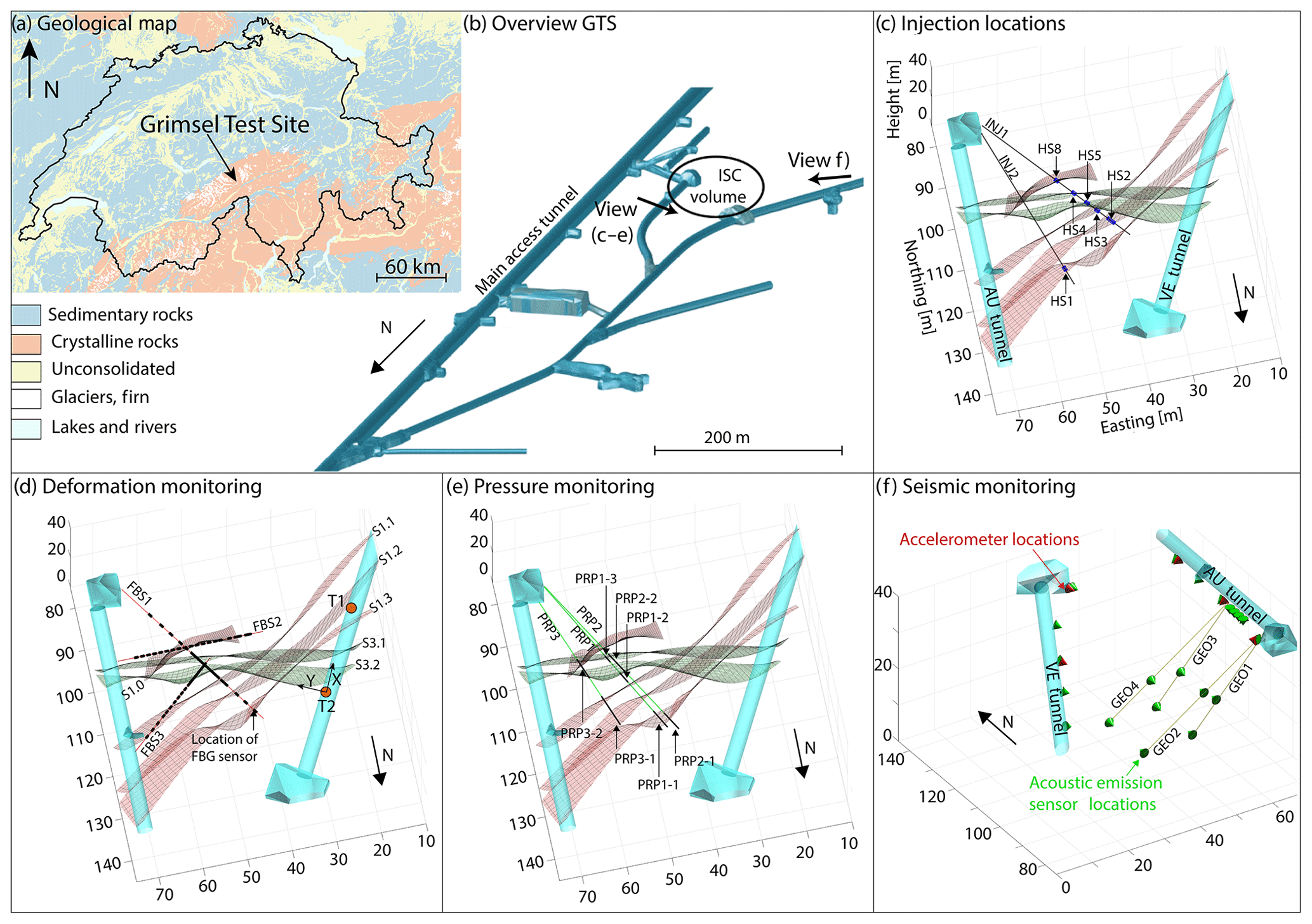
Figure 1Location of the GTS in Switzerland indicated in the geological map (a) and the location of the test volume within the GTS (b). Panel (c) shows the location of the injection intervals together with the target shear zones. Panel (d) illustrates locations of the strain sensors and tiltmeters, with indicated tilt axes, and labels the target shear zones. The pressure monitoring intervals are shown in (e), and the station locations of the seismic monitoring network are indicated in (f). More details on the monitoring setup can be found in Doetsch at al. (2018a).
The GTS is located in crystalline rocks and has an overburden of ∼480 m. The early Permian rocks (Grimsel Granodiorite and Central Aar Granite) intruded the crystalline crust 299±2 Myr ago (Keusen et al., 1989; Schaltegger and Corfu, 1992) and are close to the mineralogical transition between granodioritic and granitic rocks (Wenning et al., 2018). The rock mass in the test volume contains a pervasive foliation with an average orientation of 140/80 (i.e., dip direction/dip) (Krietsch et al., 2018b). In addition, the rock mass is intersected by two sets of shear zones (see Fig. 1c–f) that differ in their genetic history and present-day architecture. The older set, referred to as S1, contains four subparallel shear zones (Fig. 2a), which includes few poorly hydraulically connected fractures (Brixel et al., 2020b) with an average orientation of 142/77 (Fig. 2c). The younger set, referred to as S3, includes subparallel shear zones with an average orientation of 183/65 (Fig. 2b). Within the test volume, the two present S3 shear zones coincide with a meta-basic dyke each which accommodated most of the past deformation. Optical televiewer (OPTV) images suggest that the rock mass between the two S3 shear zones is intensely fractured (>20 fractures per borehole meter). This has been confirmed by geophysical imaging (Doetsch et al., 2020). Thus, this zone differs from the relatively undisturbed rock mass surrounding these shear zones, which has one to three fractures per meter (Krietsch et al., 2018b). During the deformation history of the rock mass, the S1 shear zones were sheared in a right-lateral manner by the S3 shear zones. Therefore, the S1 shear zones and the fractures included therein can have a local orientation that is subparallel to S3.
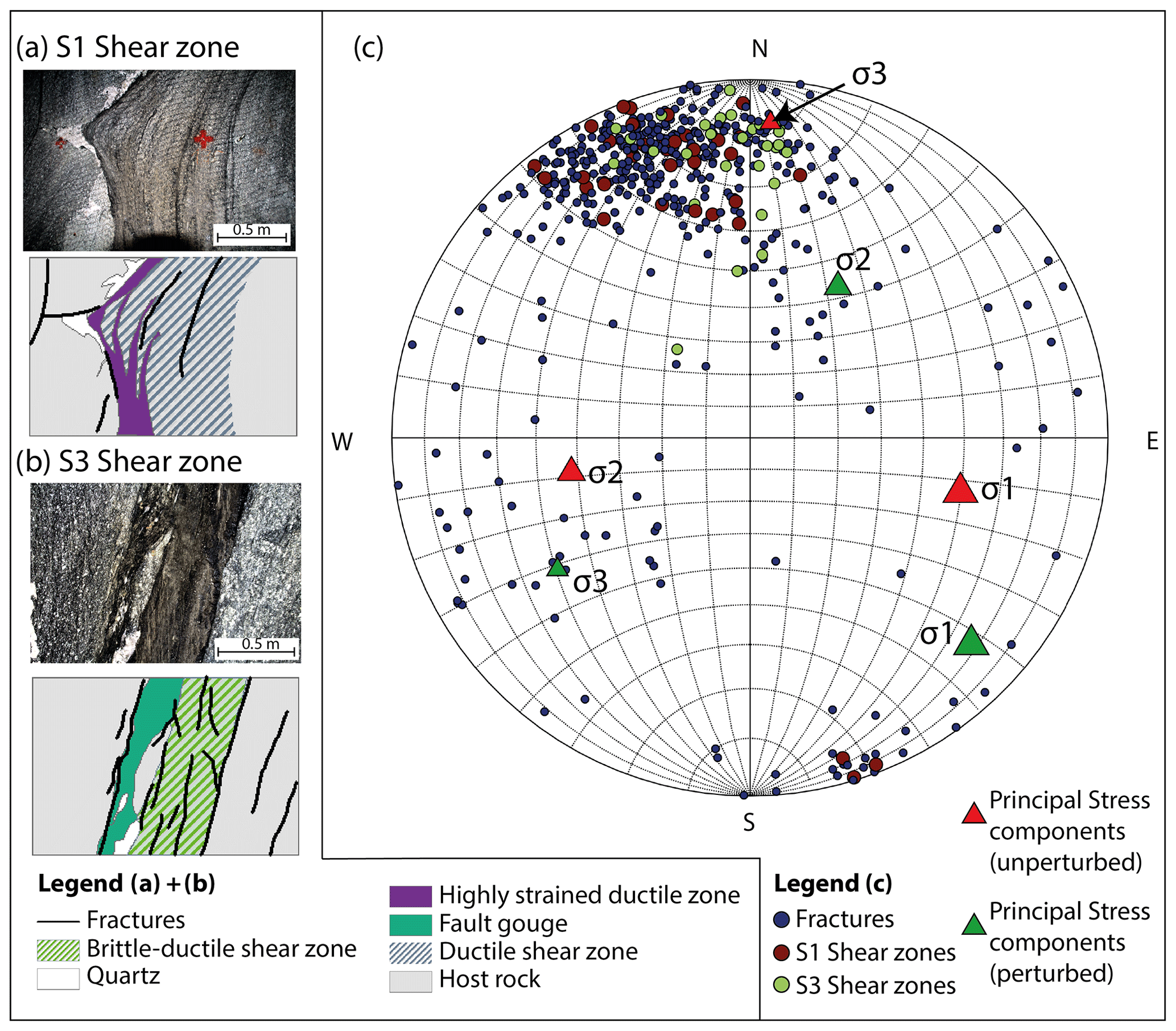
Figure 2Photographs (upper image) and interpretations (lower image) of the S1 (a) and S3 (b) shear zones as seen at the AU tunnel wall (modified after Krietsch et al., 2018b). (c) A lower hemisphere stereo net showing the poles of all mapped fractures and shear zones. The orientations of the principal stress components from the unperturbed and perturbed tensor are also shown.
In addition to the geological characterization, the in situ stress field was characterized prior to stimulation within the test volume by Krietsch et al. (2018c). A progressive stress field perturbation to an otherwise relatively uniform “far-field” stress state was observed. It begins 11 m from the shear zones as they are approached from the south (Krietsch et al., 2018c). The estimated unperturbed far-field principal stress magnitudes (measured 40 m away from the target shear zones) are 13.1 MPa (σ1), 9.2 MPa (σ2) and 8.7 MPa (σ3). At a distance of ∼5 m from the shear zone the principal stress magnitudes dropped to 13.1 MPa (σ1), 8.2 MPa (σ2) and 6.5 MPa (σ3). In addition, the principal axis orientations differed from those of the unperturbed tensor (this solution is referred to as the perturbed tensor; Fig. 2c). As the shear zone is approached, σ3 declines to as low at 2.9 MPa immediately before the zone. Although the perturbed stress tensors have been measured closer to the target stimulation volume and shear zones, the unperturbed stress tensor is also considered in our analyses; through the conceivable substantial stress heterogeneities, it remains unclear whether the perturbed or unperturbed stress tensor explains our observations better.
The unperturbed stress tensor would imply that the shear stresses acting on the S1 shear zones tend to be higher than those acting on the S3 shear zones, whereas they are similar for the perturbed stress tensor (Fig. 3). We assume that the perturbed stress tensor is better representative for locations near the stimulation injection well and the unperturbed stress tensor for the far field.
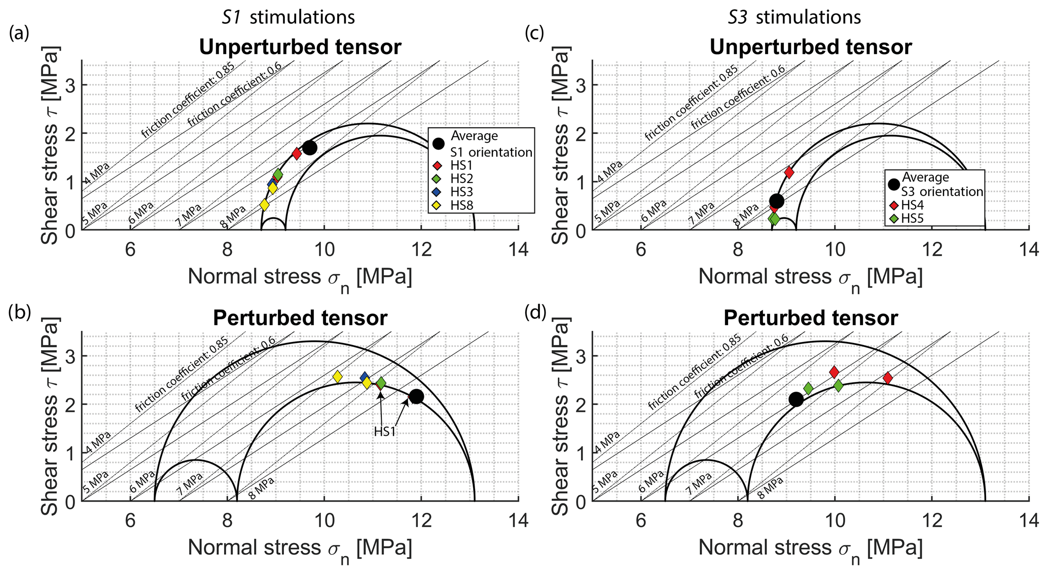
Figure 3Stress states associated with the perturbed and unperturbed tensors for S1 and S3 shear zones. The implied average shear and normal stresses acting on the S1 and S3 shear zones (estimated over all mapped borehole intersections of these shear zones) are indicated in black. Also shown are the shear and normal stress acting on the principal fractures imaged in the S1 and S3 intersections with INJ boreholes. Additionally, a range of injection pressures is indicated as a black-lined failure criterion with different friction coefficients.
The ISC test volume can be accessed from three tunnels. A total of 12 boreholes were drilled into the test volume for high-pressure fluid injection (referred to as INJ boreholes) and monitoring of pressure (PRP boreholes), strain (FBS boreholes) and seismicity (GEO boreholes) (Fig. 1).
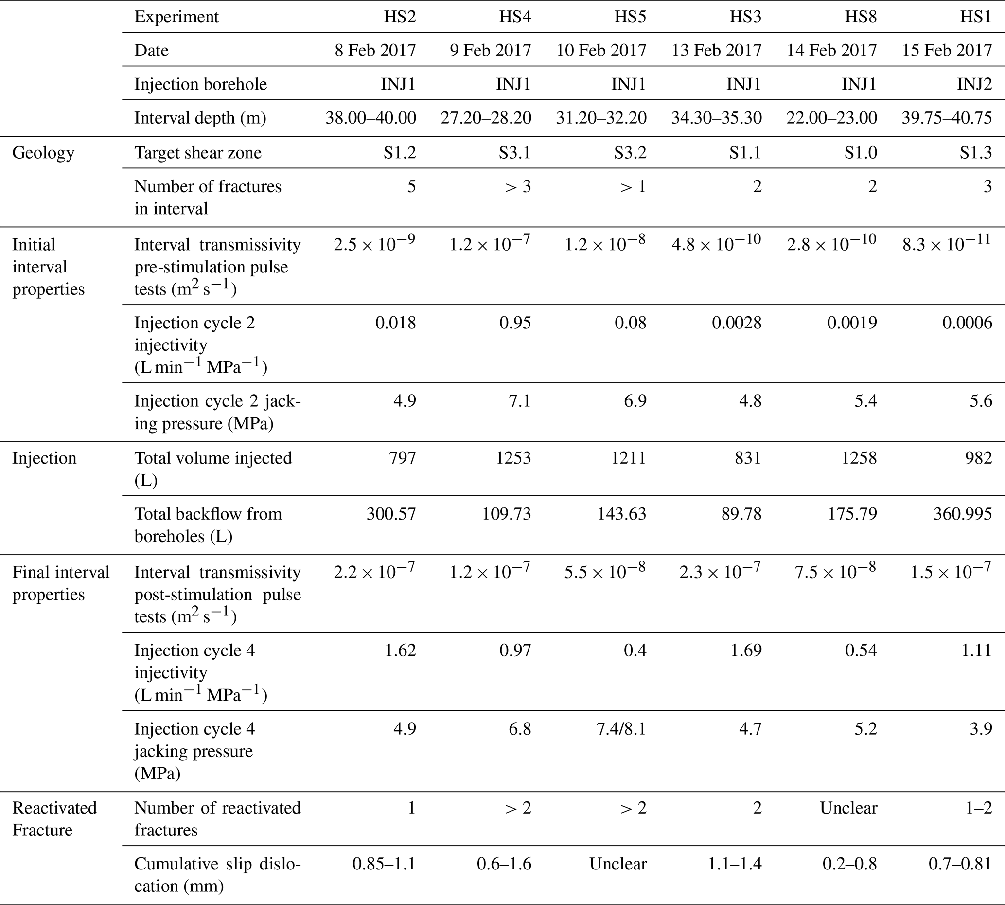
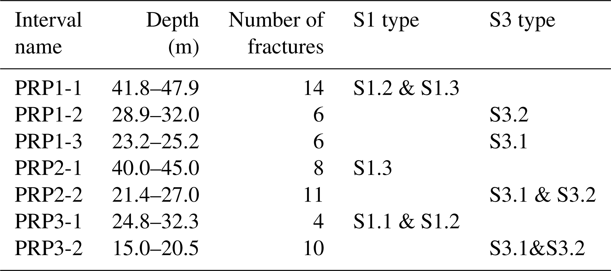
The six stimulation experiments targeted the four S1 shear zones and two S3 shear zones along the INJ boreholes (Table 1 and Fig. 1c). The injection intervals for the stimulation experiments were defined on the basis of optical televiewer (OPTV) images and the 3D geological model by Krietsch et al. (2018b). They had a length of 1 or 2 m and covered the target shear zones plus adjacent fractures. To quantify the near-wellbore transmissivity changes in the intervals resulting from the experiments, low-pressure (Pinjection<0.5 MPa) hydraulic tests consisting of pulse and constant rate injections were conducted before and after the hydraulic stimulation campaign in each injection interval (Brixel et al., 2020a, b; Jalali et al., 2018a, b). The hydraulic properties of the intervals (i.e., transmissivity, storativity and wellbore storage) were estimated using the numerical simulator nSight1.
Table 1Overview of the stimulation experiment with corresponding information about the injection interval in chronological order.
3.1 Injection protocol
The standardized protocol consisted of four injection cycles, which each consisted of progressively increased pressure or flow rate steps (Fig. 4). In all cases, the steps were kept constant until quasi-steady-state flow conditions were reached. The first two cycles were step-pressure injections and were intended to estimate the pre-stimulation jacking pressure and injectivity of the injection interval. Here, the first cycle serves to break down the injection interval so that the near-wellbore fracture responses during subsequent cycles are largely elastic. The third cycle was a step-rate injection that constituted the actual stimulation. The majority of the fluid volume was injected during this cycle and was intended to propagate the stimulation effects away from the injection well. The last cycle was performed to estimate the post-stimulation jacking pressure and injectivity and began under pressure control but then switched to flow rate control to obtain higher flow rates in the last two injection steps. Each injection cycle was followed by a shut-in phase and a subsequent venting phase. During venting, the pressure lines were opened to the atmosphere in the AU tunnel for 20 to 40 min. However, the lines leading to the pressure monitoring intervals were opened only after the actual stimulation phase and the final injection cycle for intervals that showed a significant pressure change. Thus, the induced fluid pressure disturbances within the fractures of the rock mass were partly, but not entirely, drained at the beginning of each injection cycle. Following each experiment, all intervals were allowed to drain for a minimum of 12 h before the next experiment. The total volume of fluid injected in each experiment was limited to approximately 1000 L to ensure low seismic hazard and few disturbances to nearby experiments (Gischig et al., 2016). The backflows from the injection borehole and all pressure monitoring intervals were measured during the venting phases.
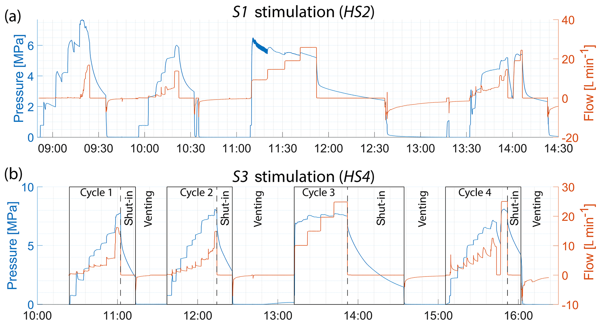
Figure 4Injection protocol for (a) experiment HS2, which targets S1 structure S1.2, and (b) experiment HS4, which targets S3 structure S3.1. The various phases of the four cycles performed in each experiment are indicated in (b). Similar plots for all other intervals are presented in Fig. A2 of the Appendix.
3.2 Monitored properties at the injection well
Hydraulic jacking pressure and injectivity were determined from a P–Q cross-plot of the test data, on which P presents the injection pressure and Q is the injection flow rate. Each point denotes the flow and pressure values at the end of each step when quasi-steady-state conditions are reached, typically after 10 min. The injectivity of the test interval is taken as the ratio between the flow rate and injection pressure at low injection pressures when mechanical effects are negligible. The intersection of the low-pressure linear trend with the pressure axis defines the initial formation pressure. Dahlø et al. (2003) noted that there is no consensus as to which feature in the P–Q plot provides the best estimation of the jacking pressure (i.e., the normal stress across the fractures that supports the lowest normal stress) because it is unclear at which point along the steepening P–Q curve the compliant fracture response turns into liftoff of the fracture surfaces. We take our best estimate of the jacking pressures before and after the stimulation as the intersection of the low- and high-pressure trends of the second and fourth cycles, respectively. In both these cycles it is assumed that the response of the fracture network to the step increases in pressure is purely elastic and repeatable. Therefore, the low-pressure injectivity was also derived from the second and fourth injection cycle (Figs. 6 and A3 in the Appendix). In addition, we picked the injection pressure limit during the actual stimulation (injection cycle 3) for all experiments (Fig. A3).
The induced slip dislocation within the injection intervals were estimated from acoustic televiewer (ATV) logs that were run before and after each HS experiment. The ATV probe has a travel time precision of 0.1 µs, yielding a radius precision of 0.07 mm for borehole fluids with a P-wave velocity of 1483 m s−1. The travel time precision of the ATV decreases as the measured amplitude of the received P-wave decreases. Thus, the precision strongly decreases as the borehole wall becomes very rough or the borehole radius becomes strongly elliptical (Moor and Valley, 2018). Since the S3 shear zones are located in weak meta-basic dykes, which appear rougher at the borehole walls than the S1 shear zones, the radius resolution is lower for S3 shear zones than for S1 shear zones. By comparing the pre- and post-stimulation geometry of the borehole cross section across fractures it is possible to determine whether dislocation has occurred and estimate the relative displacement vector (Cornet et al., 1998; Evans et al., 2005b). To enable comparability between the images, all logs were recentralized using an ellipse fit function. Afterwards, a difference log was produced for each test interval by subtracting the pre-stimulation log from the post-stimulation log. In this difference log, a positive caliper change at a location along the borehole wall indicates that the location has moved away from the borehole axis during stimulation (Fig. 5b). The resolved radius changes can be due to (a) stimulation-induced fracture reactivation (i.e., sinusoidal traces along the borehole wall; see Fig. 5c – HS2) or (b) damage along the borehole wall (i.e., diffuse traces; see Fig. 5c – HS4). To validate the orientations and locations of reactivated fractures, the ATV logs were compared with the brittle fractures mapped in the optical televiewer images.
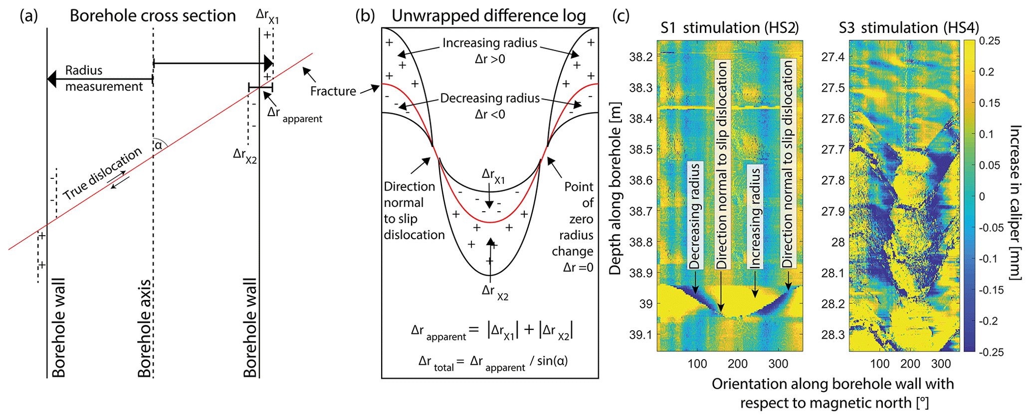
Figure 5(a) Illustration of the travel time (i.e., radius) measurement of an ATV log across a sheared fracture. (b) Observation of slip displacement direction and apparent magnitude estimate visualized in the unwrapped difference log. (c) Difference logs for HS2 and HS4 experiments. A clear trace of a reactivated fracture is visible in the HS2 log, whereas a diffuse trace with potential borehole wall damage is shown in the HS4 log.
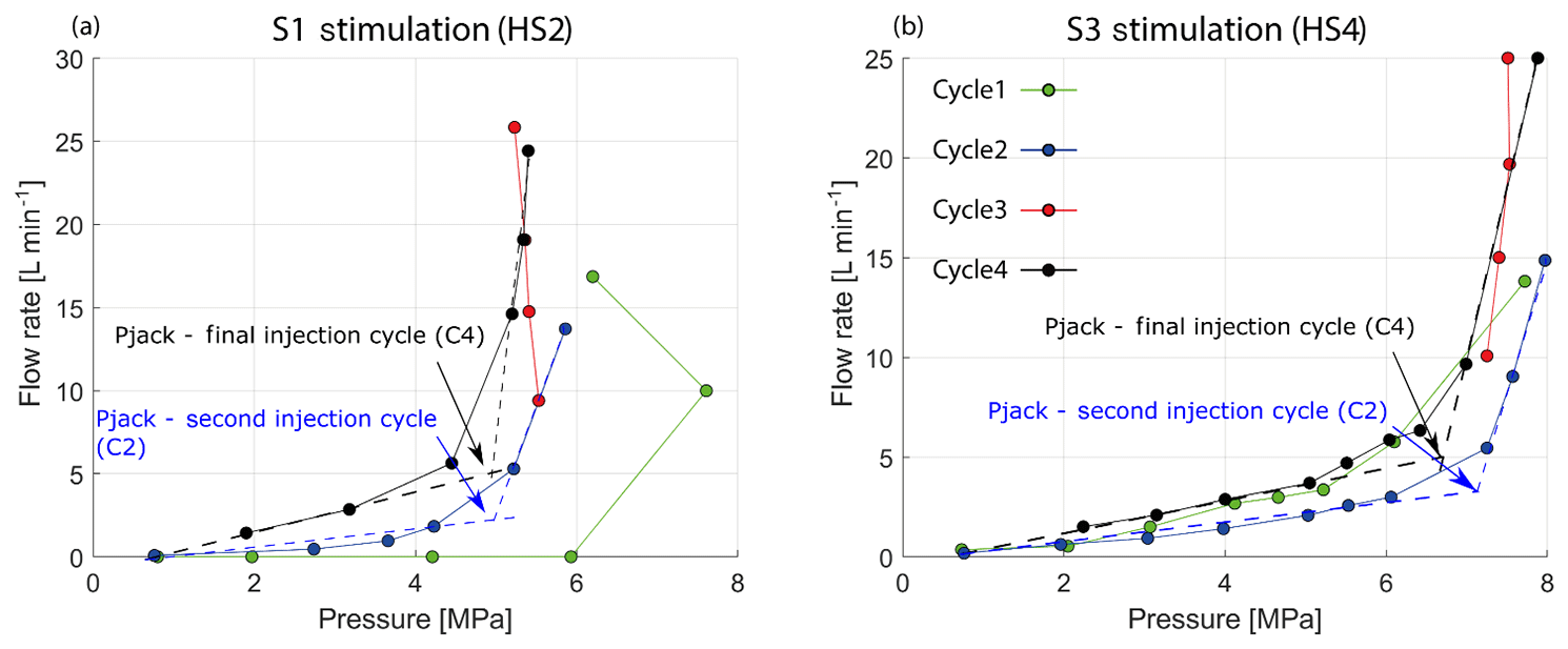
Figure 6Cross-plots of flow versus pressure data for the four injection cycles of the S1 and S3 stimulation experiment in (a) and (b), respectively. The points defining the curves for each cycle denote flow–pressure data pairs defined at the end of each step of the test in question. The first cycle frequently reaches high pressures, which may reflect the inelastic processes of the breakage of cohesive bonds and/or the slippage of fractures supporting shear stress. In subsequent cycles, the response to pressurization is largely elastic and reversible.
To estimate the magnitude of slip dislocation across a reactivated fracture, the areas of radius increase and decrease are mapped along the fracture trace (Fig. 5b). The sum of the absolute maximum radius changes on both sides of the fracture (i.e., ΔrX1 and ΔrX2) revealed the apparent amount of slip dislocation (Δrapparant). Since the radius changes are measured normal to the borehole axis, the true slip dislocation Δrtotal is calculated by correcting the apparent dislocation Δrapparant with respect to the intersection angle between the borehole axis and the fracture plane (α).
Along the sinusoidal trace of the reactivated fracture within the difference log, the radius change varies from positive to negative and back. The location at which these radius change variations occur (Δr=0) is normal to the direction of induced permanent dislocation (Fig. 5b).
3.3 Pressure monitoring
The three PRP boreholes were equipped with customized grouted packer systems to continuously monitor fluid pressure in a total of seven intervals within the test volume (Fig. 1e). The pressure monitoring intervals were named according to the borehole name and the interval number counted from the borehole bottom upwards (e.g., PRP2-1 is the lowermost interval in PRP2). The intervals were chosen to cover the different target shear zones in the volume (Table 2). The distances between the monitoring intervals and the injection locations are listed in Table A2 in the Appendix. The packer system consists of a grouted section (uppermost part), the open pressure monitoring intervals (two to three per borehole), resin sections in intervals without pressure monitoring, and inflatable packers to seal off the monitoring intervals. The packers have a length of 0.2 m and were inflated with pressures between 2 and 3 MPa. The seven intervals were connected to pressure sensors in the AU tunnel through saturated polyamide lines of 2 mm o.d. The sensors used were Keller PAA33-X transmitters that had an accuracy of 0.025 MPa. A detailed description of this packer system can be found in Doetsch et al. (2018a).
In addition to the fixed pressure monitoring intervals in the PRP holes, a double-packer system was installed in one of the two INJ boreholes that was not used for injection. The system allowed pressure to be monitored between the two packers, and between the lower packer and borehole bottom. Similarly, the pressure was also monitored between the lower packer and the borehole bottom in the INJ borehole that was used for injection. The packer systems in the INJ holes were moved for each experiment to allow injection into and monitoring of the target shear zone (Table A1).
3.4 Deformation monitoring
3.4.1 Strain monitoring
The three FBS boreholes were dedicated to longitudinal strain monitoring (Fig. 1d). Borehole FBS1 intersects all target shear zones, FBS2 is parallel to the S3 shear zones, and FBS3 is subparallel to the S1 shear zones. A total of 20 longitudinal fiber Bragg grating (FBG) strain sensors (type os3600 by Micron Optics Inc.) were installed in each of these boreholes. The sensors were placed along sections with intact rock, as well as with single or multiple fractures (Doetsch et al., 2018a; Krietsch et al., 2018b). Subsequently, the sensors were grouted in place. The FBG sensors have a base length of 1 m and recorded strain signals with a resolution of 1 micro-strain (µε) at a sampling frequency of 1000 Hz.
As the first processing step, the data were averaged over 1 s intervals before recording, giving a sampling rate of 1 Hz and an improved resolution of 0.1 µε (Krietsch et al., 2018a). Temperature corrections were not required for the FBG data since the injected fluid had the same temperature as the rock mass and temperature variations within the rock volume were negligible. To quantify deformation, we follow the geomechanics convention and take the compressional strain as positive.
3.4.2 Tilt monitoring
Two horizontal biaxial inclinometers (type A711-2 by Jewell Instruments) were installed at the bottom of approximately 50 cm deep boreholes drilled on the floor of the VE tunnel (T1–T2 in Fig. 1d). They monitor the deviation from horizontal in two orthogonal axes with an accuracy of ∼0.5 microradians (µrad) at a sampling rate of 100 Hz. The tilt data were processed with a low-pass Butterworth filter with 100 Hz cutoff, which enhances resolution to ∼0.05 µrad. The instruments were oriented such that the x axis was parallel to the tunnel axis and the y axis normal to it. A positive tilt signal on the x axis implies the tunnel floor has dipped towards SWS, and a positive signal on the y axis implies a dip towards ESE (i.e., towards the test volume) (Fig. 1d). Instrument T2 is placed near the intersection of the tunnel with the two S3 shear zones, S3.1 and S3.2, and instrument T1 lies some 13 m to the south near the intersection of the tunnel with the S1 zones S1.2 and S1.3. The tiltmeters were covered with styrofoam balls to minimize temperature effects.
3.5 Seismic monitoring
A total of 18 piezoelectric acoustic emission (AE) receivers (type Ma-Bls-7-70m by GMuG) were installed along the tunnel walls around the test volume. Additionally, eight sensors of the same type were deployed in four dedicated boreholes (i.e., referred to as GEO boreholes; Fig. 1f). The eight borehole sensors are closest to the injection locations (3–25 m distance) for all six experiments. The sensors have a bandwidth of 1 to 100 kHz. Additionally, five calibrated one-component accelerometers (type 736T by Wilcoxon) were collocated with the five AE sensors at the tunnel wall for magnitude calibration purposes.
Seismic data were recorded continuously throughout the experiments at a sampling rate of 200 kHz using a 32-channel acquisition system with 31 active channels. Induced seismic events were located using an anisotropic velocity model based on manually picked P-wave onsets. For more details on the seismic monitoring and event localization, see Doetsch et al. (2018a), Gischig et al. (2018) and Villiger et al. (2020).
Given the large volume of data recorded, we will for the most part restrict ourselves to illustrating the hydraulic and mechanical observations using the figures for two stimulation experiments as representative for all six hydraulic shearing experiments, which are documented in the Appendix. We use the experiments called HS2 and HS4 as representatives for stimulations that targeted S1 and S3 fault zones, respectively.
4.1 Near-wellbore observations
The initial injectivity and near-well transmissivity for the S1 intervals were systematically lower than those for the S3 intervals by 1–3 orders of magnitude (Table 1). Despite this difference, the post-stimulation transmissivities were remarkably similar, all lying between and m2 s−1. Thus, substantial transmissivity increases of up to 3 orders of magnitude were realized for the S1 shear zones, whereas the increases for the S3 shear zones were limited to less than an order of magnitude (Fig. 7). The final low-pressure injectivities, measured during the last injection cycle, ranged 0.4–1.7 L min−1 MPa−1 (Table 1).
The initial jacking pressures in the two injection intervals covering S3 shear zones are systematically larger than those for the S1 shear zones, in most cases by ∼1.5 MPa. Following the stimulations, four of the intervals showed the same or slightly reduced jacking pressure, with one showing a significant decrease (S1 stimulation − HS1) and one a significant increase (S3 stimulation − HS5) (see Table 1). The final jacking pressures for the S1 intervals varied between 3.9 and 5.5 MPa, whereas for the S3 intervals the variation was 6.8 and 7.4 MPa. As opposed to S3 intervals, the maximum recorded interval pressure during cycle 1 in S1 intervals exceeded the jacking pressure.
An upper limit of injection pressure despite increasing flow rates (referred to as pressure-limiting behavior) was observed during the main stimulation injection cycle in all experiments, with some slight systematic differences between the S1 and S3 intervals. For the S3 stimulations, a slight increase in pressure with increased flow rate was evident, as the P–Q curves become progressively steeper with increased flow rate when a pressure limit was approached on the final step (Fig. 6). In contrast, the P–Q curves for the S1 stimulations showed pressure monotonically declining with higher flow rate in some cases (i.e., HS2, HS3) and declining before recovering in others (e.g., HS1, HS8). As for the jacking pressures, the maximum injection pressures attained in the stimulation injections were consistently higher for the S3 shear zones than for S1 shear zones (Table 3).
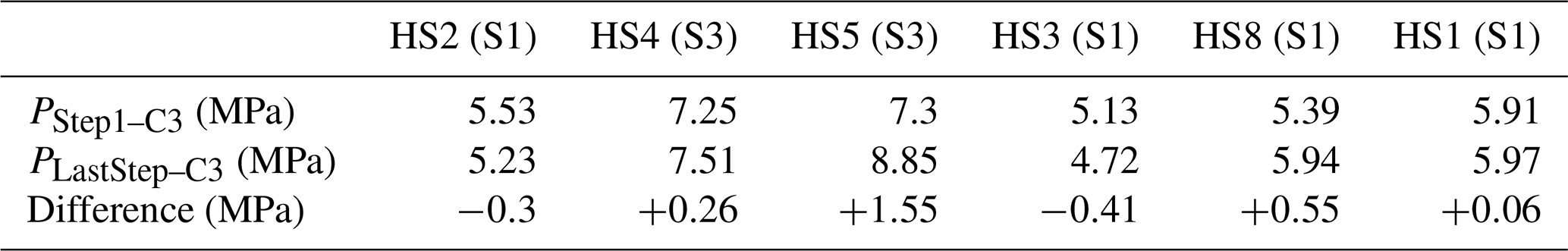
Table 3Injection pressures measured at the end of the first and last (before shut-in) injection steps of the stimulation injection cycle (C3). The difference between the two values is listed in the lower row.
The resolved slip was localized on a single fracture, as in HS2, or distributed over various fractures as in HS4 (Fig. 5). The maximum value of ∼1.4 mm was found for an S1 stimulation (HS3 in Fig. 7d). Dislocations slightly less than a millimeter were also identified for other stimulated S1 shear zones (HS1 and HS2, and perhaps also HS8), although the uncertainty is large. A value of ∼1 mm was obtained for an S3 stimulation (HS4), but the uncertainty in this estimate was large because of the greater borehole wall roughness at the S3 shear zones (Fig. A4). The direction of the slip vector could only be determined for two zones: for HS2 it was 261/02 (i.e., dip direction/dip), and for the two reactivated fractures in HS3 it was 264/01 and 286/04. All three fractures were reactivated in a right-lateral strike-slip dislocation in an east–west direction.
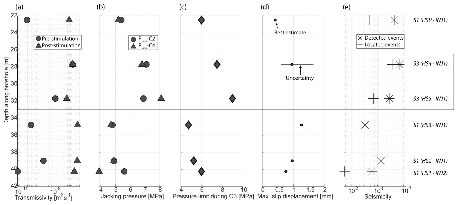
Figure 7Hydromechanical responses of the target intervals to the stimulation experiments. Indicated are (a) pre-and post-stimulation transmissivity, (b) pre- and post-stimulation jacking pressure (Pjack–C2 & Pjack–C4), (c) the injection pressure limit observed during C3, (d) estimated cumulative slip displacement, and (e) the number of detected and located seismic events.
4.2 Fluid pressure inside the rock mass
No systematic differences in the recorded pressure magnitude responses to injection into S1 and S3 shear zones were evident away from the injection well. The highest fluid pressure perturbations were detected in monitoring intervals that cross the target shear zones. Transient fluid pressure perturbations were observed on almost all PRP pressure monitoring intervals during all six stimulation experiments. In four experiments, the pressure increases rarely exceeded 1 MPa, even though peak injection pressures ranged 5–9 MPa (Figs. 8 and A5). However, fluid pressures up to 6.7 and 4.2 MPa in magnitude were observed during an S3 stimulation (HS5) and an S1 stimulation (HS8), respectively (Fig. A5). These perturbations were only seen in a few pressure monitoring intervals during these two experiments. Although one of the monitoring intervals that detected the strong pressure signals covered the target shear zone that was being injected (i.e., PRP1-2 during HS5), the remainder of the strong responses were from intervals that covered other zones, indicating that the shear zones are interconnected.
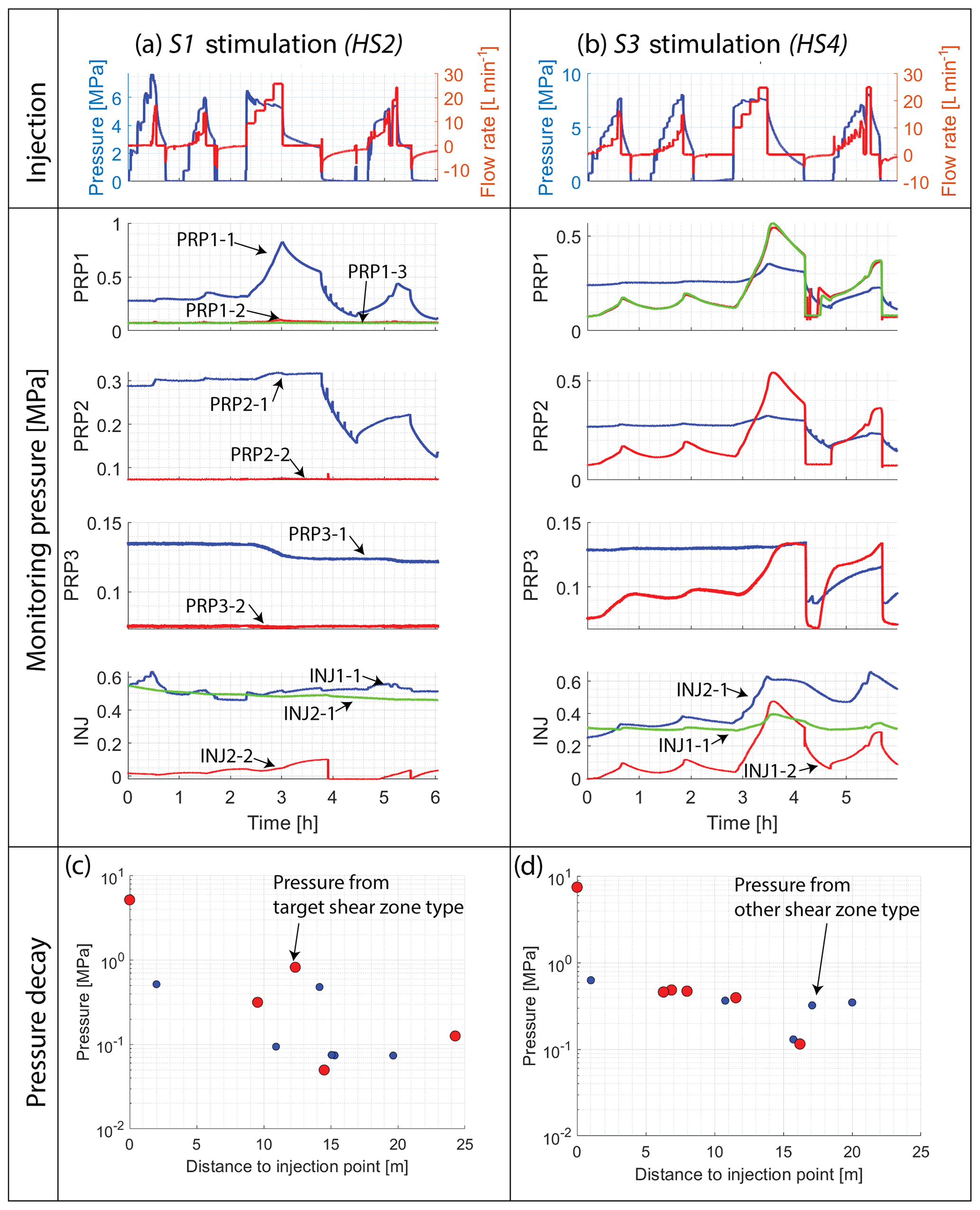
Figure 8Pressure data for HS2 and HS4 are shown in panels (a) and (b), respectively. Injection protocols for both experiments are shown at the top. In the middle, the corresponding time series of pressure recorded at the various intervals of the PRP boreholes are plotted. Panels (c) and (d) show the pressures prevailing in the intervals at the end of the final step of the stimulation injection cycle plotted against the distance to the injection point for HS2 (a) and HS4 (b), respectively.
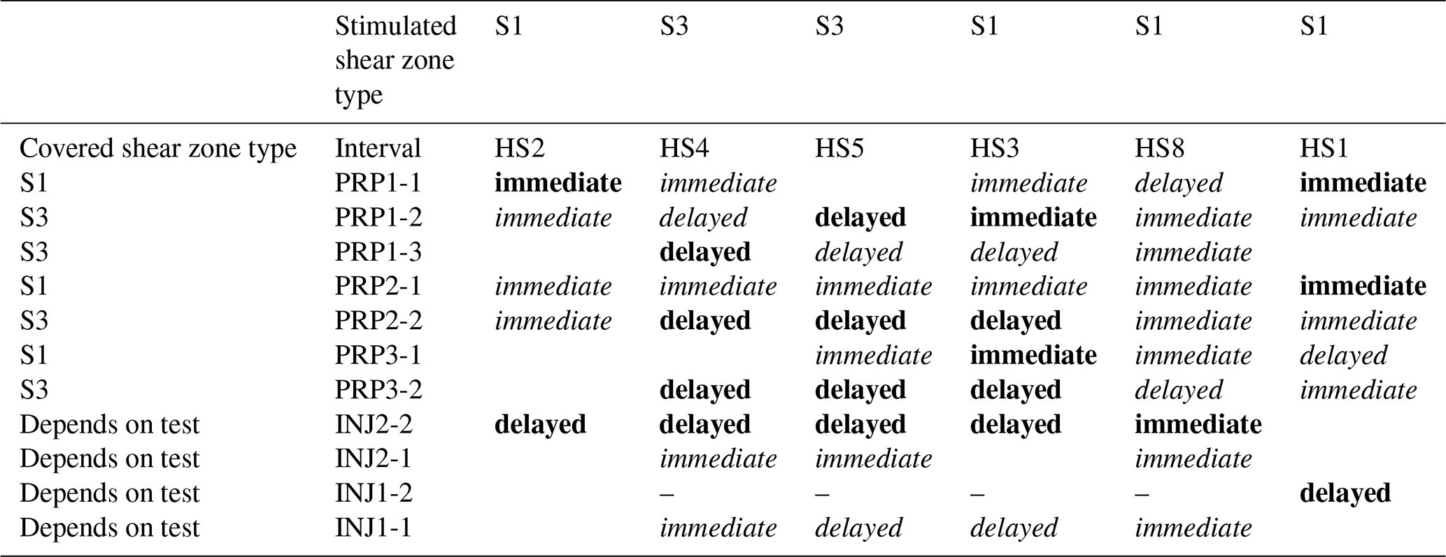
A tendency for the pressure in the PRP intervals to react more immediately to shut-in after injections into S1 intervals compared to S3 intervals can be discerned, particularly at the end of the stimulation injection cycle (Fig. 8 and Table A3). The immediate pressure response of S1 shear zones (e.g., PRP1-1) to shut-in after injection into another S1 shear zone (e.g., HS2) contrasts with the delayed reaction of pressure intervals sampling S3 structures (PRP1-3 and PRP2-2) that were target during HS4 stimulation (Fig. 8). Indeed, for the S3 stimulations, almost all monitoring intervals that included the target shear zone showed a delayed response to the shut-ins.
The fluid pressure in most monitoring intervals at the end of the experiments remained perturbed from their initial values but in all cases had returned to initial values by the start of the subsequent experiment the following morning (Fig. A5). The pressures prevailing in PRP1-1, PRP2-1 and PRP3-1 at the end of the experiments were below the initial values due to the effect of venting the intervals following the stimulation injection cycle and last injection cycle (Figs. 8, A5). The venting responses of intervals covering the S1.3 shear zone (PRP1-1 and PRP2-1) consistently differed from all other intervals in that significant backflow occurred during venting so that the interval pressure declined relatively slowly. In contrast, the pressure in all other intervals declined rapidly to the atmospheric pressure in the tunnel when the valve was opened, although it was clear in some cases that backflow into the interval was occurring as the pressure began to climb once the valve was closed (e.g., S1 covering pressure interval PRP3-1 in HS4) (Fig. 8). Thus, backflow into S1 intervals upon venting tended to be greater than that for intervals cutting S3 fracture zones.
Pressure perturbations were also detected at remote monitoring intervals. The largest distance to injection was 25 m for PRP1-1 during HS8 (Fig. A6e) and typically 15–19 m for the other stimulations (Figs. 8 and A6). These distances are Euclidean distances. Thus, the true distances of pressure diffusion along hydraulically active fluid pathways might be underestimated. No systematic difference in pressure transmission distances for S1 and S3 stimulations was evident. For both shear zone types, the pressure perturbations registered in intervals that cut the target shear zone tended to be greater than at other intervals located at a comparable distance. For HS4, however, a relatively weak response was observed at an interval (PRP3-2) that covered the shear zone into which the fluid was injected (Fig. 8).
4.3 Spatial–temporal rock mass deformation
During all experiments, the FBG sensors measured compressional and extensional strain perturbations in response to the injections. The largest strain magnitudes were observed during periods of fluid injection, and the magnitudes decreased during shut-in and venting (see Fig. 10a–b for experiments HS2 and HS4). For each strain signature, we define the permanent (i.e., irreversible) strain as the strain remaining at the end of the experiment and the reversible strain as the difference between the peak strain and the permanent strain (Fig. 9). Here, the peak strain corresponds to the largest strain excursion in the coda and may be positive (i.e., compressional) or negative (i.e., extensional). In most cases, the peak strain was observed during the stimulation injection cycle, C3 (Fig. 9a–b), when the largest amount of fluid was injected. Generally, we observed that the reversible strain amplitudes were often larger than the irreversible amplitudes (Table 4). Nonzero permanent strains were detected for each experiment on all operational gauges.
Table 4Ratio between reversible peak strain magnitude (εrp) and permanent strain magnitude (εp) averaged over all operational gauges and all experiments.
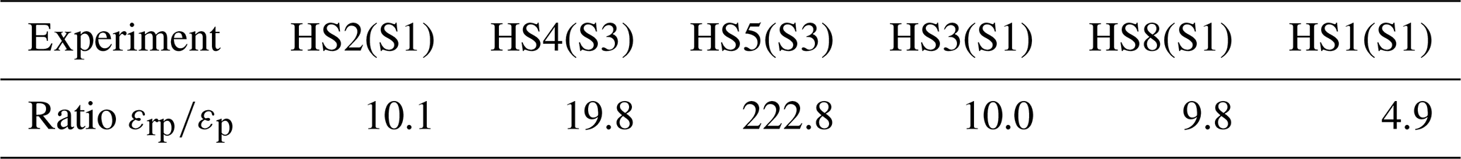
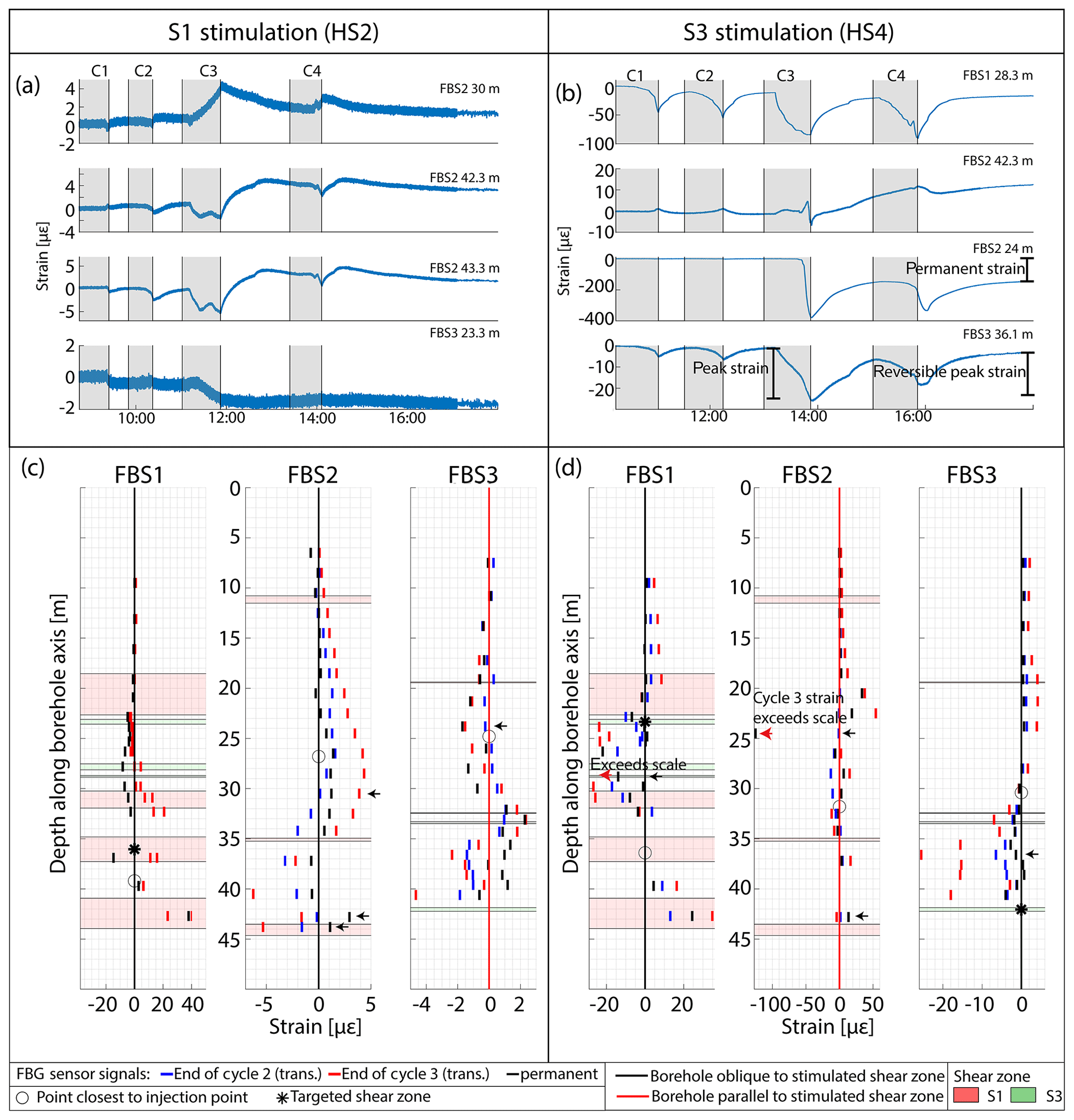
Figure 9(a, b) Examples of strain time series from four FBGs during HS2 and HS4, respectively. The vertical shading denotes periods of injection during the four cycles. Examples of the permanent strain, the peak strain and the reversible peak strain are indicated on the HS4 strain codas. (c, d) Profiles of permanent strain and strain at the end of the injection phases of C2 and C3 along the three FBS boreholes for HS2 and HS4, respectively. The open circle along each borehole denotes the location closest to the injection point for the experiment in question. The pink and green bands indicate places where the holes cut S1 and S3 shear zones, respectively. The small black arrows indicate the sensors whose strain codas are shown in (a) and (b).
4.3.1 Strain along borehole axis
Profiles of strain signals picked at the end of the C2 and C3 injections and permanent strains are shown along the three FBG borehole axes in Figs. 9 and A7. Spatial coherence between neighboring gauges is evident along the strain profiles, although heterogeneity is also present that in some cases appears to be related to shear zone intersection points (Figs. 9 and A7).
Within boreholes that are parallel to target shear zones (i.e., FBS3 for S1 stimulations and FBS2 for S3 stimulations), extensional strains were measured at the locations along the borehole axes that lay closest to the injection locations (Figs. 9 and A7). This extension in most cases transitioned into compression within 5 m either up or down the boreholes from this point. In contrast, boreholes that are subnormal to the target shear zone (i.e., FBS1 and FBS2 for S1 stimulations and FBS1 and FBS3 for S3 stimulation) tended to show compressional strains near the point closest to the injection location (note that this point is not necessarily the borehole intersection of the target shear zone).
4.3.2 Extent of deformation field
Figures 10 and A8 show the absolute amplitude of the strain signals as a function of distance from the strain gauge to the injection point for the end of injection C3 and permanent deformation after stimulation. In most experiments, a general tendency for lower strain amplitudes at greater distance is evident (Figs. 10 and A8), with strain signals larger than 1 µε furthest from the injection locations. Thus, the overall extent of the mechanically effected zone was larger than 27–33 m with respect to radial distance to the injection point. In the near field to the injection location the FBG sensors showed complex signals, which included either extension or compression (or a transition between both with ongoing stimulation) depending on the orientation of the sensor axes and location with respect to the target shear zones. With increasing distance from the injection location, the strains in most cases tended to be compressional (Figs. 10 and A8). The transition from this compressional field to a mix of compression and extension (i.e., complex strain field) seemed to occur at slightly larger distances from the injection point for S1 than S3 stimulations during C3 (Table 5).
Table 5Distance of strain transition zone (change from a variable to compressional strain field) to the injection point measured at shut-in of injection cycles 2, 3 and 4.
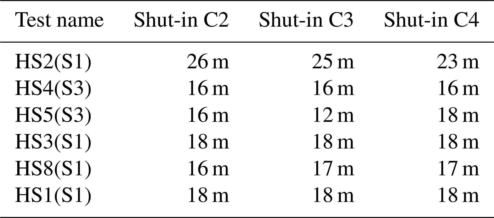
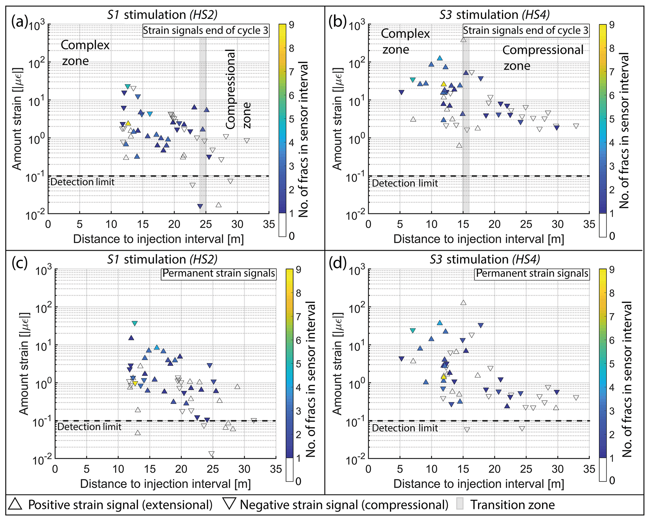
Figure 10Strain signals with respect to distance to the injection point for HS2 and HS4. Generally, the strain perturbations prevailing at the end of the injection phase of cycle 3 were compressive beyond a certain distance, which varied between experiments. This distance is denoted by the vertical grey line in (a) and (b) and separates the compressional zone from the so-called “complex zone” wherein a mix of extensile and compressive strains is observed. The color code of the triangle indicates the number of fractures located within the FBG sensor intervals.
The floor of the VE tunnel underwent tilting during all experiments, with the magnitudes ranging from −4 to 2 µrad (i.e., to ∘) for both tilt axes (Figs. 11 and A9). Nearly immediate tilt responses were seen at the start and stop of injection in most cycles and most experiments. The largest tilt signals for each experiment tended to be observed on the instrument closest to the shear zone targeted for stimulation (Fig. A9). Specifically, for injections into the S1 shear zones, significantly larger signals were seen on instrument T1 than T2. The sense of the tilt indicated that the tunnel floor tilted away from the target S1 shear zone towards WNW during the stimulations. During the S3 stimulation HS4, the tunnel floor near T1 tilted temporarily towards east (i.e., towards the test volume), whereas the tunnel floor near T2 tilted towards the west (i.e., away from the test volume). However, the permanent tilts at T1 and T2 both indicated tilting towards the east with a similar magnitude. During the other S3 stimulation (HS5), T1 showed tilting to the NW, whereas T2 indicated tilting the SW, with no significant permanent tilt on either instrument. Thus, the transient tilts at both locations indicate similar E–W components of tilting of the tunnel floor away from the test volume but with opposite north–south components (Fig. A9). Significant permanent tilts remained only after the two S1 stimulations (HS2 and HS1). In general, the transient tilt signals were often much more pronounced than the permanent signals.
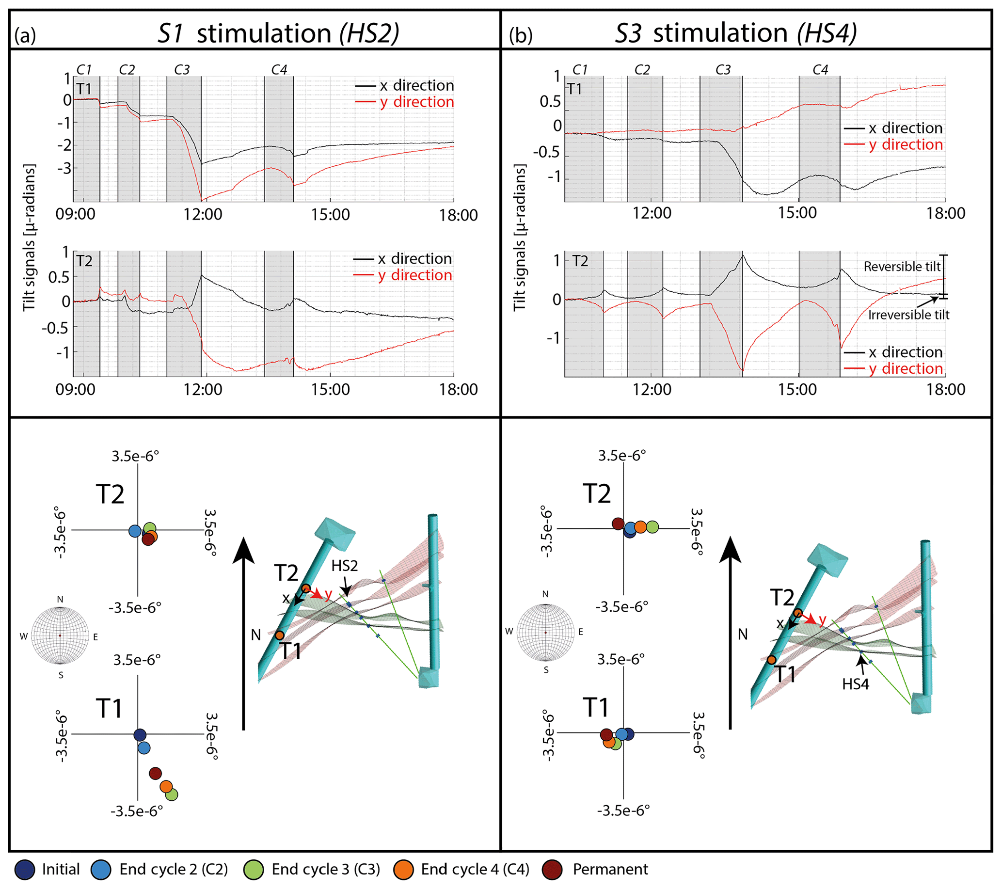
Figure 11Inclinometer data for an S1 stimulation (HS2) (a) and S3 stimulation (HS4) (b). The upper part of each panel shows the tilt time series for both experiments with the injection periods marked by the shaded vertical bands. The lower part of each panel shows for each experiment on the right side a horizontal cross section through the study volume at the level of the tunnels. In these sections, the shear zones, the injection locations, and tiltmeter T1 and T2 positions are indicated. The x and y axes of the tilt data are indicated on T2. Axes orientations of T1 are the same. Changes in the downward-oriented normal vector of the tunnel floor at T1 and T2 are shown in the lower hemisphere plots at the left of the frames. These frames are zoomed-in sections to the very center of the lower hemisphere stereo net. Thus, the axes appear as a Cartesian coordinate system.
During the stimulation injection cycle of an S3 stimulation experiment (HS4) the FBG sensor installed at 24 m of depth in FBS2 indicated strong (up to µε peak strain) localized extension (Fig. 12). No macroscopic fracture was evident on the OPTV images of the sensor location prior to the experiment. The large extension at 24 m began abruptly near the end of the stimulation injection cycle when the flow rate was stepped from 20 to 25 L min−1 and rapidly developed at rates up to −1.2 µε s−1. Following the experiment, the sensor showed a permanent strain of −120 µε, implying a reversible peak strain component of −250 µε. This large extensile strain at 24 m coincides with the development of moderately large compressive strains recorded by the FBGs at 20 and 22 m, as well as a complex reversal of an initial extensile strain to result in a compressive permanent strain at 26 m. Following injection, all strains progressively decayed to leave a permanent strain. Similar strains responses on the four sensors were observed during the subsequent final injection cycle (C4).
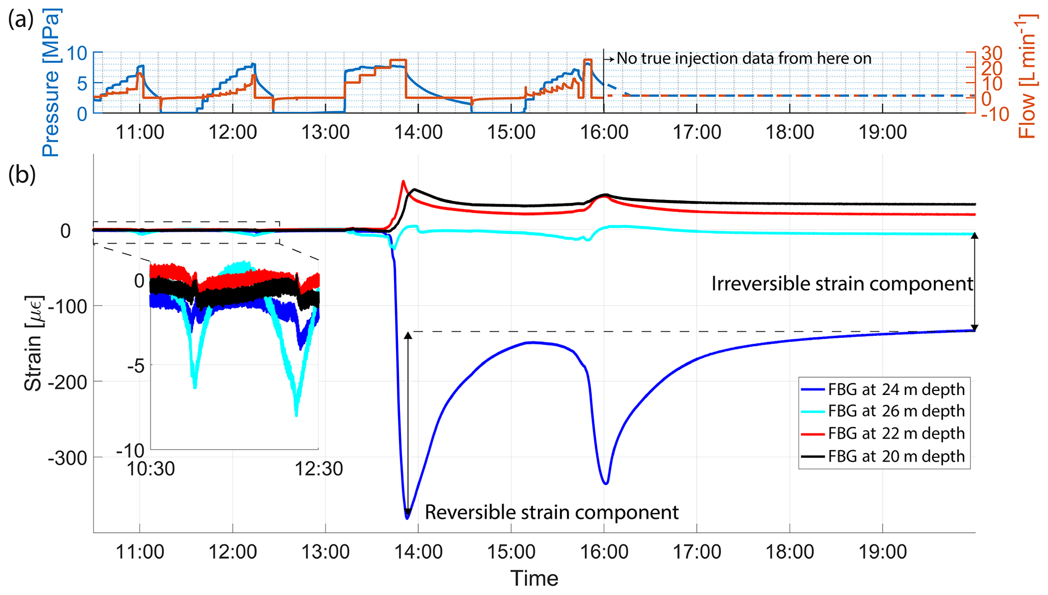
Figure 12(a) Injection protocol during the stimulation experiment of interval HS4 with interpolations as a dashed line after the experiment. (b) Strain records at four neighboring FBG sensor locations in FBS2 during HS4. The inset shows the stains at an expanded scale during the first two cycles.
5.1 Reactivation of preexisting fractures
Stress information retrieved from the injection and pressure observations at the injection interval revealed a distinct behavior of S1 and S3 stimulations: during the first injection cycle of S1 stimulations, the peak injection pressure exceeded the jacking pressure and the maximum injection pressure of the stimulation cycle (i.e., limiting pressure). This indicates that S1 shear zones had a tensile strength component that had to be overcome to open the fracture. This was not observed during S3 stimulation. Such tensile strength at S1 shear zones is consistent with the observation that S1 shear zones had much lower initial transmissivity compared to S3 shear zones (Fig. 7). Prior to the stimulations, the jacking pressures of the two S3 intervals were systematically higher (∼ 7–8 MPa) than the values obtained for the S1 intervals (∼5 MPa). For all experiments, an injection pressure limit was observed during the stimulation cycle, which we interpret as liftoff of fractures (Pearson, 1981). Again, the limiting pressure was systematically higher for S3 stimulation (7–9 MPa) than for the S1 stimulation (5–6 MPa). We interpret this as higher normal stress acting across S3 shear zones than across S1 shear zones. This disagrees with the stress tensors established by Krietsch et al. (2018c) (Fig. 3), from which one would expect slightly higher normal stress across S1 than across S3. Further, the expected normal stresses would be higher (>8.5 MPa for the unperturbed stress tensor and >10.5 MPa for the perturbed stress tensor) than observed during the stimulations. We explain this inconsistency with stress heterogeneity in the stimulated rock volume (note that the perturbed stress tensor has been measured at about 40 m from the stimulated rock volume). Indeed, during the stress measurements a jacking pressure of 3 MPa was obtained at the margins of the S3.1 structure, which is lower than across the same structure at the INJ1 borehole.
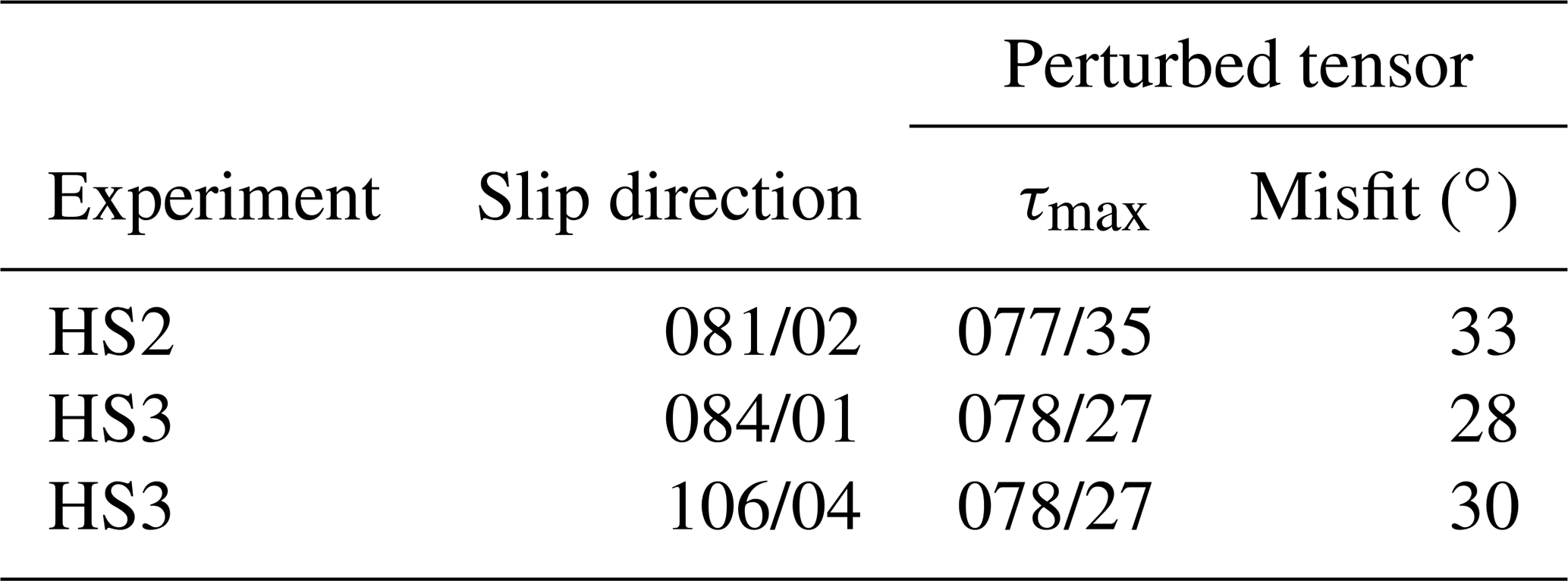
The induced slip displacements imaged at the injection intervals occurred along single or multiple fractures (Figs. 5 and A4). The number of reactivated fractures was larger for the initially high transmissive S3 intervals compared to the initially low transmissive S1 intervals. In all cases with multiple reactivated fractures, one fracture trace experienced distinct large shear dislocation, similar to that observed by Evans et al. (2005b) for the Soultz-sous Forêt stimulation projects. The slip direction of each reactivated fracture was compared with the direction of the maximum shear stress vector resolved for the individual fractures using the perturbed stress tensors. The angle between the maximum shear stress vectors and the azimuth of induced slip dislocations varied between 28 and 33∘ (Table 6). Thus, the derived slip direction corresponds to right-lateral shear sense, while the predictions of the stress tensor measured nearby point to oblique right-lateral shear sense with a thrust faulting component. The angular misfit might be explained by a transient local stress transfer between adjacent fractures during fluid injection at the injection well (Kakurina et al., 2019). However, stress heterogeneity, as already inferred above, may also explain why slip directions are not well predicted by the measured stress tensor.
Given the different architectures and properties of the S1 and S3 shear zones, stress heterogeneity is expected. High fracture densities and the presence of meta-basic dikes produce elasticity contrasts around the S3 shear zones (Doetsch et al., 2020). Enhanced foliation and associated elastic anisotropy have been measured for the S1 shear zones (Krietsch et al., 2018b; Doetsch et al., 2020). Additionally, these material properties not only vary between shear zone types, but also laterally along individual shear zones (see seismic velocity distributions along S3 shear zones; Doetsch et al. 2020). Thus, we argue that stress variations related to material contrasts (changes in both magnitude and stress rotation) give rise to larger changes in normal stress along the different shear zones types than their orientation in a constant stress field.
Table 6Orientation of slip dislocation on the fractures estimated from the pre- and post-stimulation ATV logs and the maximum shear stresses resolved on the fractures from the perturbed stress tensor. All orientations are given as dip direction/dip.
5.2 Near-wellbore transmissivity enhancement
We found that the near-wellbore transmissivity enhancement was most efficient for structures that had low initial transmissivities. After stimulation, the near-wellbore transmissivities were similar in magnitude for all experiments. This may reflect an upper limit on shear-induced irreversible transmissivity enhancement. Lee and Cho (2002) found similar effects in laboratory experiments, which suggests that achievable shear-induced transmissivity enhancement depends on the height of asperities along the fracture surface. Nonetheless, in our case, the magnitude of transmissivity enhancement depends on the architecture of the stimulated structures. Stimulation of the intensely fractured rock mass around S3 shear zones was associated with only limited transmissivity enhancement, while the less intensely fractured S1 shear zones contributed larger transmissivity enhancement. We argue that stimulation of long open-hole sections would have led to less advantageous stimulation outcomes. Prior to stimulation, the fractures in all intervals differed in near-wellbore transmissivities but had similar slip tendencies (Fig. 3). Thus, a combination of low-transmissivity structures (i.e., S1 shear zones) in the same packer interval with initially high-transmissivity structures (i.e., S3 shear zones) would not have led to a transmissivity enhancement of the low-transmissivity structures because the highly transmissive structures would have taken most of the injected fluid. This highlights the advantage of short injection intervals over long open-hole injections.
5.3 Complex flow field
The monitored pressure signals indicated that the pressure diffused predominantly along the target shear zones, similar to observations of stimulations at other EGS sites (e.g., Evans et al., 2005a). Because individual fractures associated with the target shear zone often intersected the same pressure monitoring intervals as the target shear zones, it was impossible to resolve which portion of the pressure signal propagated along which individual fracture. We observed rapid increases in high fluid pressures (i.e., on the order magnitude of the injection pressure) only during one S1 and one S3 stimulation (HS8 and HS5, respectively; Fig. A5). During most experiments and the majority of monitoring intervals, the pressure signals are far below the injection pressure and rarely exceed 1 MPa (Fig. A5). These findings are somewhat unexpected: according to Murphy et al. (2004), among others, fracture dilation during fluid injection leads to nonlinear pressure diffusion and promotes higher fluid pressures and pressure increases further away from the borehole than linear pressure diffusion would produce. Most pressure signals in our case resemble a linear diffusive pressure field. Nonetheless, FBG strain measurements and P–Q curves (Fig. 7) confirm that fracture dilation occurred during stimulation. Thus, our observations suggest that the flow field in the fault planes is heterogeneous and high-pressure signals away from the injection point may be limited to flow channels. As shown by Krietsch et al. (2020) flow along channels may change during ongoing injections. This observation challenges common conceptual models of stimulation treatments based on oversimplified fault geometries (i.e., single penny-shaped fracture) and pressure diffusion models (radially or spherically symmetric diffusion models) (e.g., Cappa et al., 2019).
5.4 Hydromechanical rock mass responses
Based on the observed pressure response upon shut-in, we divided our pressure signals into two different types. (1) The pressure monitoring intervals that cover the target shear zone often observed a delayed response to shut-in, indicating a diffusion-controlled pressure signal. (2) In contrast to this, pressure intervals outside the target shear zone often responded immediately to shut-in (Fig. A5 and Table A3). In some cases, this behavior was detected further away from the injection location than the diffusion-controlled signals. These signals are most likely associated with a poro-elastic far-field response (Segall, 1989)
Similarly, the observed deformation signals can loosely be divided into a near- and a far-field response. The deformations in the near field to the injection reflect stress field changes predominantly arising from effective normal stress reductions across fractures, which can produce both normal opening and also relaxation of shear stress through slip (Stein, 1999). The observed magnitude and sign (tension or compression) of these hydromechanical deformations strongly depend on the position and orientation of the strain sensor with respect to the stimulated zone. This interpretation is consistent with McClure and Horne (2014) and Rutledge et al. (2004), who note that deformations arising from mode I, II and III dislocations can occur simultaneously. It is noteworthy that the observed peak strain often far exceeds the permanent strain remaining after stimulation. This implies that the reversible component of fracture dislocation (a combination of normal and shear compliance) may be larger than the irreversible component (a combination of slip and shear dilatancy). In the near field, we also observed the formation of new fractures that propagated away from the stimulated shear zone (Fig. 12). These fractures are interpreted as tensile fractures that formed due to stress concentrations induced by shear dislocation along irregularities (asperities) of the main shear zone (McClure and Horne, 2014) or by gradients of the slip magnitude.
In the far field, i.e., outside this complex strain field, the vast majority of strain measurements show compression. We interpret these compressive signals in the far field to be produced by volumetric compression as a consequence of the volumetric expansion in the near field to the injection (Segall and Fitzgerald, 1998). The tilt signals also belong to this category of far-field responses, as they do not directly measure fluid-pressure-induced effective normal stress changes and the corresponding elastic and inelastic consequences (e.g., fracture opening and closure, slip, etc.). Similarly,the rapid pressure increases some distance away from injection may also be related to far-field volumetric compression (Segall, 1989).
5.5 Stimulated volume
Based on hydraulic and mechanical observations, we suggest two distinct zones around the injection point: (1) a complex near-field zone dominated by pressure diffusion, fracture opening, closure, shear slip and the formation of new fractures; and (2) a far-field zone dominated by stress transfer and the associated poro-elastic response (Fig. 14). Thus, we subdivide the overall effected rock volume into a primary stimulation zone, which is close to the injection point, and a secondary effected zone that captures the far-field responses (Fig. 13).
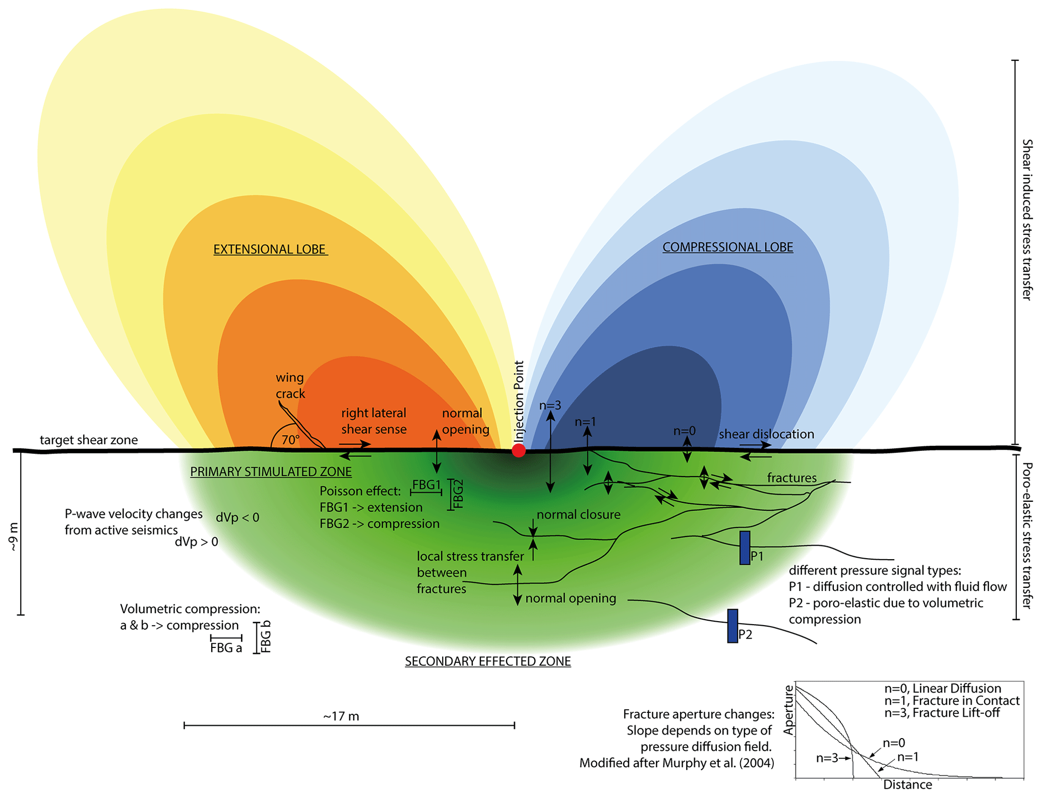
Figure 13Schematic overview of hydromechanical mechanisms active within the “primary stimulated zone” about an injection interval. The black arrows indicate fracture surface dislocations. The shape of the shear-induced stress change lobes was modified after Karakostas et al. (2014) and Preisig et al. (2015). For sake of simplicity, both the shear-induced and the poro-elastic processes are drawn individually on either side of the main fracture and not superimposed.
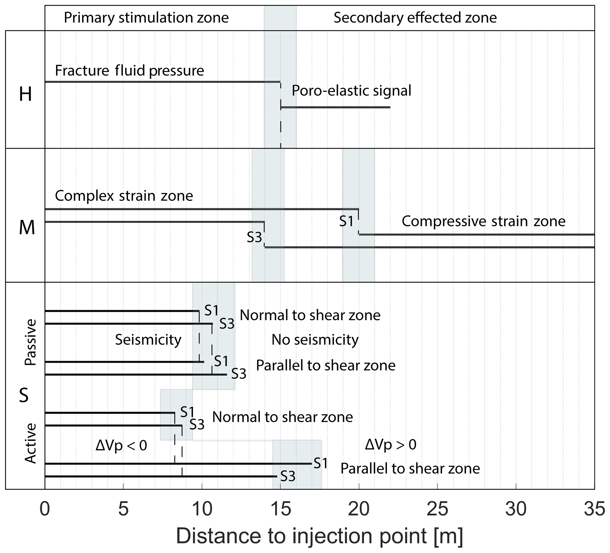
Figure 14Comparison of radial extension stimulated zones determined by hydraulics (H), deformation (M) and seismics (S). For the seismic observations, we distinguish between active seismics (velocity changes) and passive seismics (located seismic events). Note that we did not distinguish between measurement directions for the H and M estimates, as we did not have enough measurement locations to resolve them properly.
The pressure monitoring observations indicate that the radial extent of the diffusion-controlled pressure changes extended up to 15 m from the injection point (Figs. 14 and A6). Beyond this distance, between 15 and ∼22 m, the poro-elastic response was dominant. Due to the sparse monitoring, we cannot exclude the possibility that poro-elastic responses reach much further into the rock mass. The transition between the two different responses was taken as 15 m from the injection point along the shear zone. This also corresponds to the transition between the “complex” strain field, which appeared to be directly affected by active fracture slip and normal opening, and the compressional strain field, which decayed in magnitude with distance and appeared to be a far-field effect. As for the pressure, we cannot determine the outer limit of the compressional strain field because strains larger than the detection limit were observed on the most remote FBG sensors during all stimulations.
The extent of the primary stimulation zone depends on the target shear zone properties, such as initial transmissivity and the number of reactivated fractures.
5.6 Comparison between hydromechanical observations and seismic responses
Doetsch et al. (2018b) and Schopper et al. (2020) used active seismic methods to analyze P-wave velocity changes that were observed during the stimulation experiments. They found that 4D seismic tomograms allowed for the tracking of fluid pressure and strain evolution. Close to the injection location, a zone with decreasing P-wave velocities was detected that was surrounded by a zone of increased P-wave velocities. These distinct zones of P-wave velocity changes correspond to the primary stimulated and secondary effected zone. We consider the isoline marking a 0.1 % P-wave velocity decrease to denote the boundary between the two stimulated zones (Fig. 15). The extent of the boundary was measured parallel and normal to the target shear zone and was found to be elongated along the target shear zone, which is consistent with the monitored pressure perturbations. In general, the extent of the zone with decreased P-wave velocities was larger during S1 stimulations than during S3 stimulations, which is in agreement with strain field observations. Based on the active seismic observations, the primary stimulated zone can be characterized as being ellipsoidal, as inferred from the strain data.
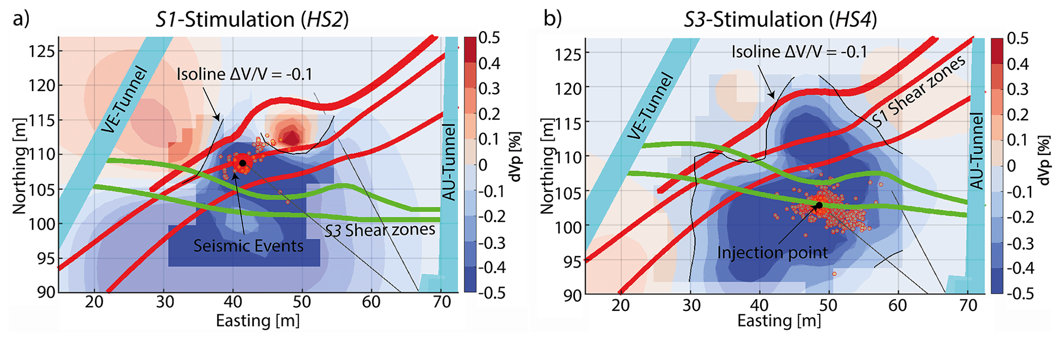
Figure 15Comparison between active and passive seismic observations during S1 (a) and S3 (b) stimulations in map view. The extent of the active seismic velocity change was traced with the −0.1 % isoline. This figure was modified after Schopper et al. (2020) and Villiger et al. (2020).
Villiger et al. (2020) analyzed the seismicity induced during the stimulation. For details on the network sensitivity and its impact on the estimate of the seismically active zones, we refer to their article published in this journal. The localization accuracy of the seismic events is better than 1.5 m. The radial extent of the clouds was found to be similar in both directions (i.e., parallel and normal) for S1 and S3 stimulations. However, more seismic events were detected along the target shear zone than normal to it. The seismic cloud has a smaller extent than the primary stimulation zone estimates from HM monitoring (Fig. 15). Thus, it seems to underestimate the total volume that has been affected by the stimulation. This agrees with the suggestion of various authors such as Duboeuf et al. (2017) and Guglielmi et al. (2015), who showed that a large portion of the stimulation-induced dislocation is aseismic. However, it disagrees with Cappa et al. (2019), who argued that seismicity is induced ahead of the hydraulically pressurized zone.
The six decameter-scale hydraulic shearing experiments conducted at 480 m of depth at the Grimsel Test Site, Switzerland, have revealed exceptional insights into the seismo-hydromechanical responses of the crystalline rock mass and fractures to high-rate injections. This was facilitated by a dense array of instrumentation installed in the test volume that included seismometers, pore pressure and strain monitoring boreholes, and inclinometers installed along tunnels. The test volume was cut by two sets of fracture zones, denoted S1 and S3, that differ in orientation and deformation history.
Data acquired with the comprehensive monitoring system in this study demonstrate the complexity of fluid flow and coupled deformations during hydraulic stimulations. For the interpretation it has to be considered that the hydraulic and mechanical data were not acquired at the same locations and thus do not directly capture couplings between the mechanical and the hydraulic response at the same location. Due to the spatial coverage of monitoring sensors it is likely that not all experiments have the same spatial data content. Further, the total size of the rock volume affected by the stimulation was not captured since the most remote strain sensors indicate deformations.
Two different shear zones sets (S1 and S3) were the target of the stimulation injections. The key results of the experiments can be summarized as follows.
Initially low-transmissivity structures were stimulated more efficiently than structures of higher initial transmissivity.
Systematically lower initial transmissivities by up to 3 orders of magnitude were observed for all four of the intervals that cut S1 target structures, with one S3 interval having a high transmissivity of 10−7 m2 s−1. Following the stimulation, all five other transmissivities were increased to this level. Evidence of shearing was seen on fractures cutting four of the six intervals but could not be linked to the transmissivity increases as the normal component of dislocation was not estimated.
Systematically higher initial jacking pressures of ∼7 MPa were found for the two S3 intervals, with the values for S1 intervals ranging between 4.8 and 5.6 MPa. With one exception, jacking pressures were unchanged by the stimulations. The measured jacking pressures are low compared to minimum principal stress magnitudes determined in the relatively undisturbed rock mass immediately to the south and almost certainly reflect strong stress heterogeneity in the decameter-scale test volume.
During the stimulation injections, hydraulic pressure propagated heterogeneously through the target shear zone. Rapid, relatively large pressure increases are interpreted as nonlinear pressure diffusion. All other pressure perturbations that had delayed arrival times had markedly lower amplitudes and could have involved linear or nonlinear diffusion. Another class of pressure perturbation seen at some measurement points outside the target zone was coincident with changes in injection and is believed to be poro-elastic in nature.
All operational FBG strain sensors throughout the study volume detected significant signals during all experiments. Generally, the signals had both reversible and permanent strain components, the former being larger than the latter. Strains measured at distances less than 15 m to the injection points were a complex mix of compression and extension, whereas only compression was measured beyond, the magnitude diminishing with distance. The complex near-field zone is believed to correspond to local stress perturbations arising from reductions of effective normal stress along fractures due to a diffusion-controlled pressure field, leading to normal and shear dislocation along fractures. The more distant compression is taken to be the response of the surrounding medium to the volume increase in the near-field volume and is a purely poro-elastic far-field effect.
The dimensions of the microseismic cloud are smaller than the dimensions of the primary stimulated zone as derived from the pressure and strain monitoring systems. We propose that this is a better measure of the stimulated volume than the seismicity cloud. The latter is also in accord with the volume of transient seismic velocity decreases as inferred from 4D seismic tomography.
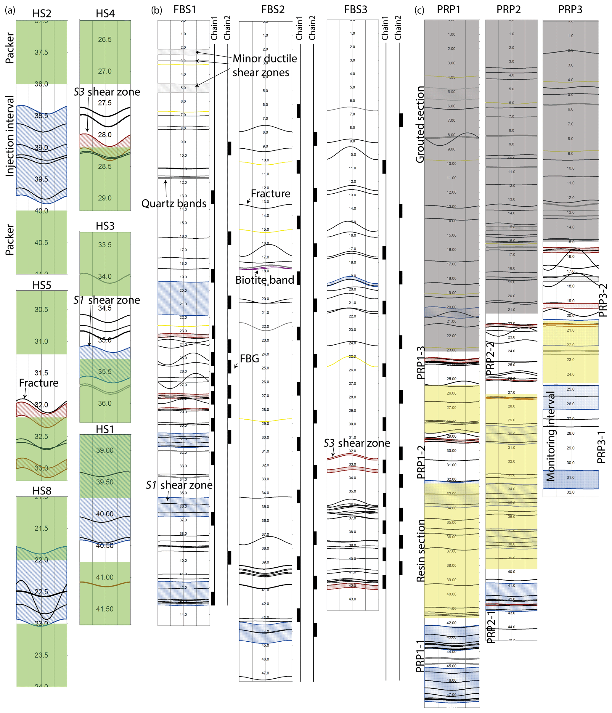
Figure A1(a) Structure logs of injection intervals, (b) structure logs of strain monitoring boreholes with sensor locations, and (c) customized packer system in the PRP boreholes, including open intervals as well as concrete and resin sections. Note that the actual packers surrounding the open intervals are not shown here due to their length of only 20 cm.
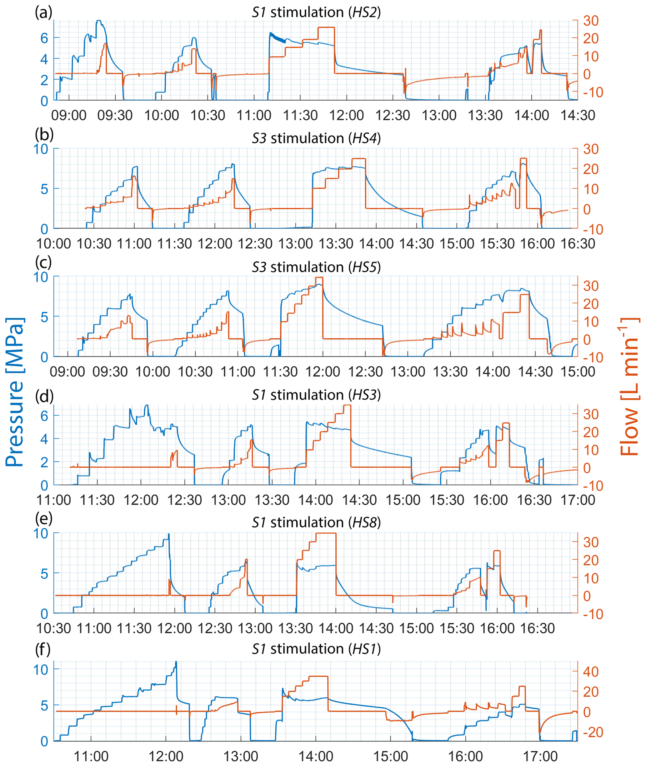
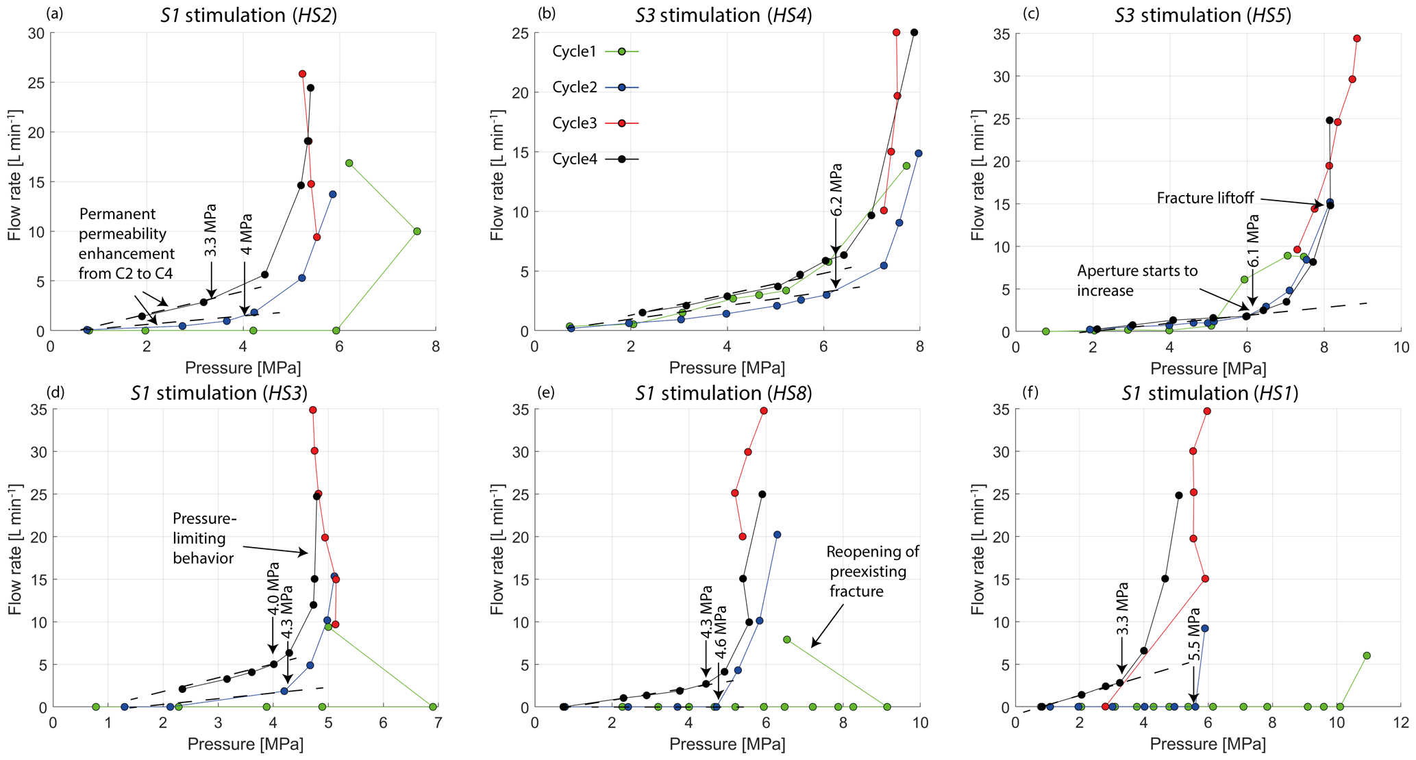
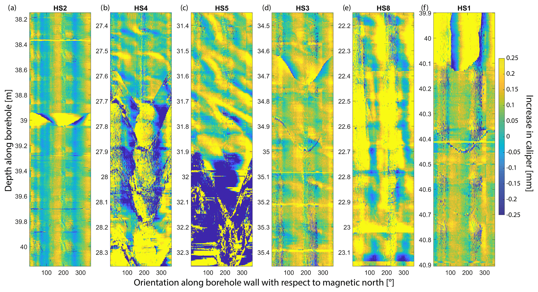

Figure A5Pressure perturbation time series for all monitoring intervals. The shut-in moments are marked as vertical lines. Note that all intervals were vented after a period of shut-in.

Figure A6Pressure signals at the moment of shut-in after C3 with respect to radial distance to the injection point.
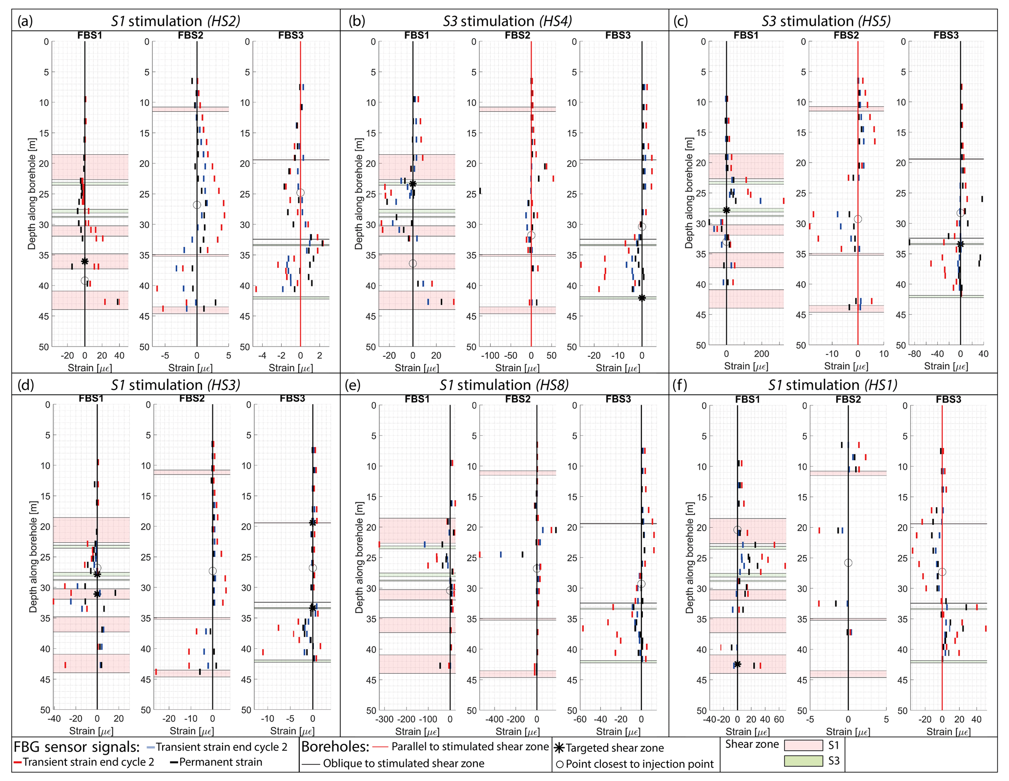
Figure A7Strain along borehole axis picked as transient at the end of injection cycles 2 and 3, as well as the permanent strain signal after the experiment.
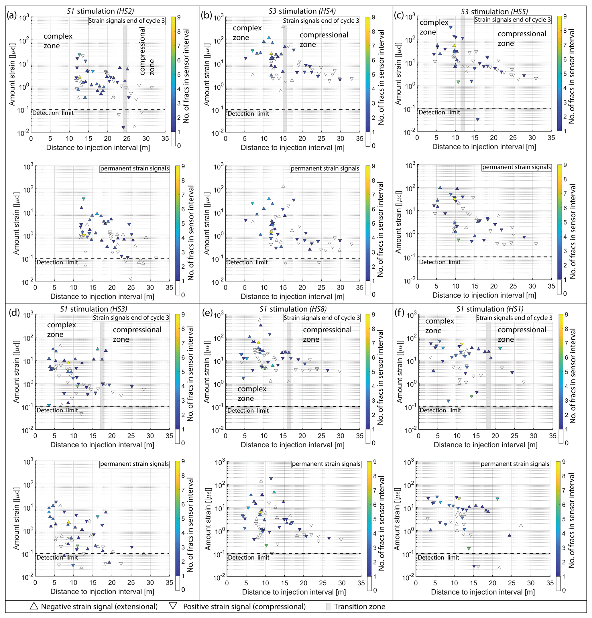
Figure A8Strain signals with respect to distance to the injection point for all experiments. The variable and compressional strain fields are labeled during C3.
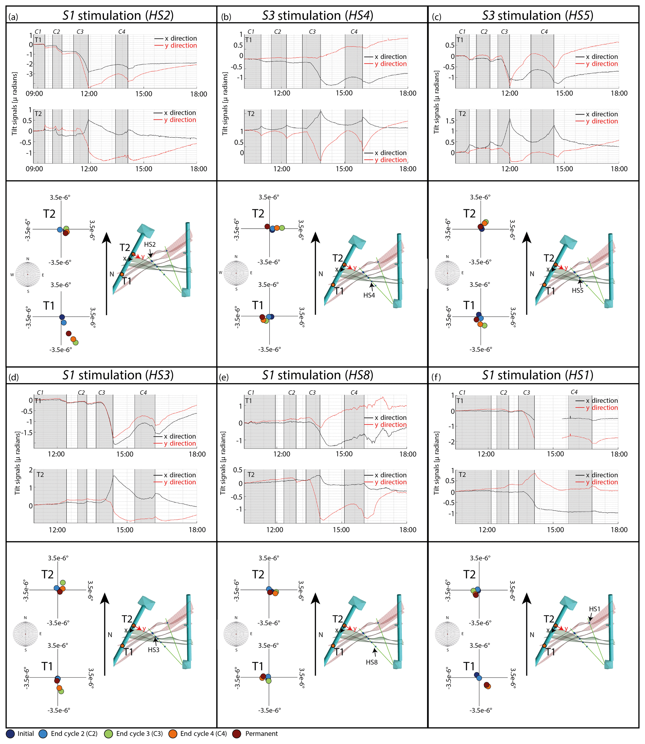
Figure A9Inclinometer data for each of the six experiments. The upper part of each panel shows the tilt time series for both experiments with the injection periods marked by the shaded vertical bands. The lower part of each panel shows a horizontal section through the study volume at the level of the tunnels, showing the shear zones and tiltmeter T1 and T2 positions. The x and y axes of the tilt data are indicated on T2. Changes in the downward-oriented normal vector of the tunnel floor at T1 and T2 are shown in the lower hemisphere plots at the left of the frames.
Table A1Locations and packed-off length of monitoring intervals in the INJ boreholes during the stimulation experiments. The fracture zones that intersect the interval are given in the adjacent column. Monitoring intervals that include the interval undergoing injection in the other INJ borehole are marked with (*).
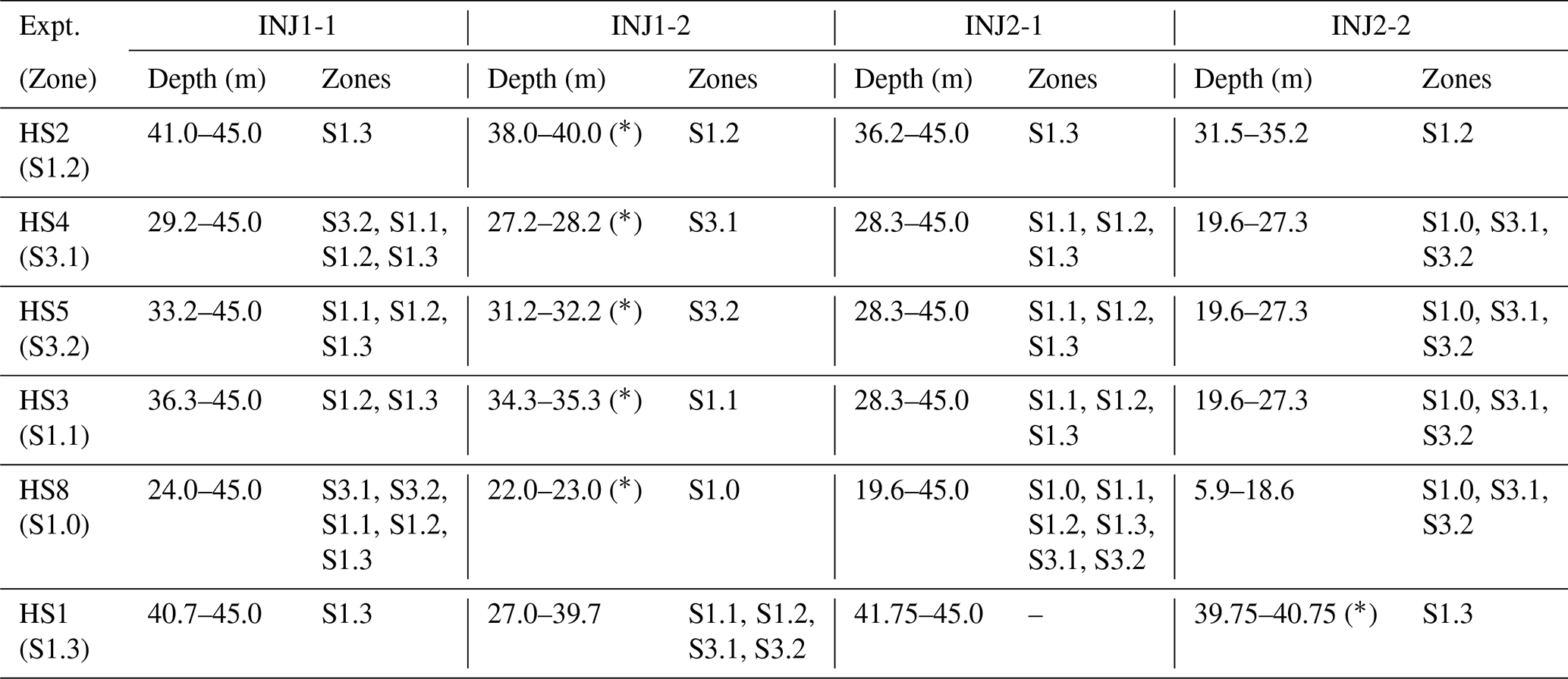
Table A2Radial distances between the midpoints of the pressure monitoring intervals and the injection interval for all HS tests. The OBS intervals represent the inactive INJ borehole.
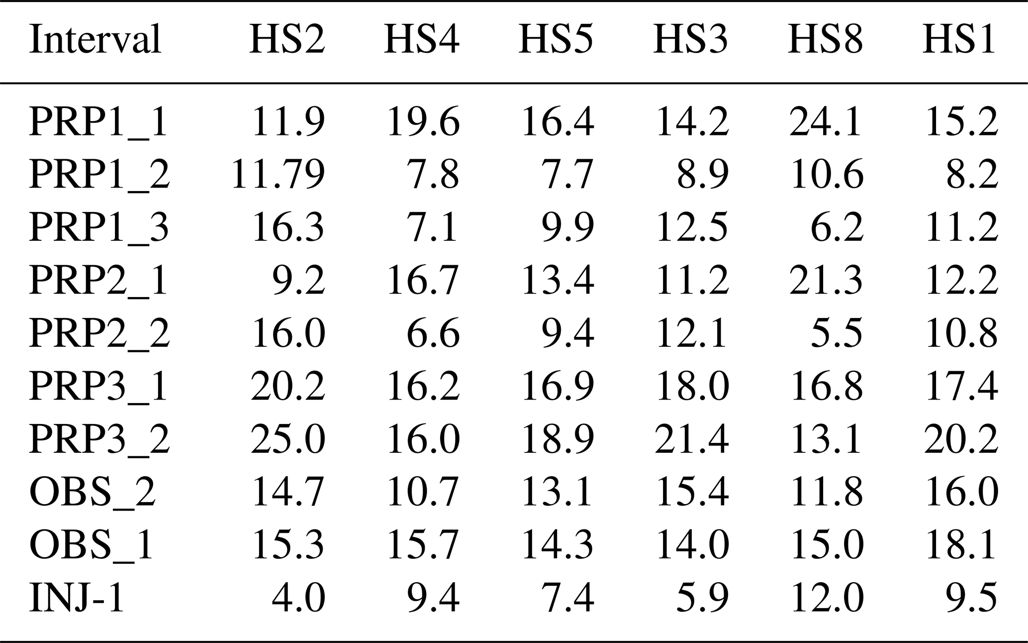
Table A3Response behavior of the pressure monitoring intervals at shut-in of injection cycle 3 for all HS tests. This table also makes the link to the shear zone targeted during each stimulation and covered by the monitoring intervals. The responses are classified as immediate (in the case of an immediate response to shut-in) and delayed (in the case of a delayed response to shut-in). The bold responses are from the intervals that covered the exact targeted shear zones. The ones in italics are taken from the intervals that do not cover the targeted shear zones.
The research data can be accessed via the ETH research collection (https://doi.org/10.3929/ethz-b-000328266; Krietsch et al., 2019).
HK, VSG, JD, LV, MJ, BV, SL and FA designed the monitoring setup. HK, VSG, JD, KFE, LV, MJ and FA conducted the experiments. HK, VSG, BV and KFE analyzed the mechanical responses. HK, MJ and KFE analyzed the hydraulic responses. JD, VSG and LV analyzed the seismic responses. All co-authors contributed to writing the paper.
The authors declare that they have no conflict of interest.
This study is part of the In-situ Stimulation and Circulation (ISC) project established by the Swiss Competence Center for Energy Research – Supply of Electricity (SCCER-SoE) with the support of Innosuisse. Funding for the ISC project was provided by the ETH Foundation with grants from Shell and EWZ as well as by the Swiss Federal Office of Energy through a P&D grant. The Grimsel Test Site is operated by Nagra, the National Cooperative for the Disposal of Radioactive Waste. We are indebted to Nagra for hosting the ISC project in their facility and to the Nagra technical staff for on-site support.
This research has been supported by the Schweizerischer Nationalfonds zur Förderung der Wissenschaftlichen Forschung (grant no. 200021_169178) and the Eidgenössische Technische Hochschule Zürich (grant no. ETH-35 16-1).
This paper was edited by David Healy and reviewed by Georg Dresen and Joerg Renner.
Amann, F., Gischig, V., Evans, K., Doetsch, J., Jalali, R., Valley, B., Krietsch, H., Dutler, N., Villiger, L., Brixel, B., Klepikova, M., Kittilä, A., Madonna, C., Wiemer, S., Saar, M. O., Loew, S., Driesner, T., Maurer, H., and Giardini, D.: The seismo-hydromechanical behavior during deep geothermal reservoir stimulations: open questions tackled in a decameter-scale in situ stimulation experiment, Solid Earth, 9, 115–137, https://doi.org/10.5194/se-9-115-2018, 2018.
Bandis, S. C., Lumsden, A. C., and Barton, N. R.: Fundamentals of rock joint deformation, Int. J. Rock Mech. Min., 20, 249–268, https://doi.org/10.1016/0148-9062(83)90595-8, 1983.
Bao, X. and Eaton, D. W.: Fault activation by hydraulic fracturing in western Canada, Science, 354, 1406–1409, https://doi.org/10.1126/science.aag2583, 2016.
Brixel, B., Klepikova, M., Lei, Q., Roques, C., Jalali, M. R., Krietsch, H., and Loew, S.: Tracking fluid flow in shallow crustal fault zones: 2. Insights from cross‐hole forced flow experiments in damage zones, J. Geophys. Res.-Sol. Ea., 125, e2019JB019108, https://doi.org/10.1029/2019JB018200, 2020a.
Brixel, B., Klepikova, M., Jalali, M. R., Lei, Q., Roques, C., Kriestch, H., and Loew, S.: Tracking fluid flow in shallow crustal fault zones: 1. Insights from single‐hole permeability estimates, J. Geophys. Res.-Sol. Ea., 125, e2019JB018200, https://doi.org/10.1029/2019JB018200, 2020b.
Brown, D. W., Duchane, D. V., Heiken, G., and Hriscu, V. T.: Mining the Earth's heat: hot dry rock geothermal energy, Springer Science & Business Media, Heidelberg, 2012.
Cappa, F., Scuderi, M. M., Collettini, C., Guglielmi, Y., and Avouac, J.-P.: Stabilization of fault slip by fluid injection in the laboratory and in situ, Sci. Adv., 5, eaau4065, https://doi.org/10.1126/sciadv.aau4065, 2019.
Cipolla, C. and Wallace, J.: Stimulated reservoir volume: A misapplied concept?, Soc. Pet. Eng. – SPE Hydraul. Fract. Technol. Conf., February 2014, 216–241, https://doi.org/10.2118/168596-ms, Society of Petroleum Engineers, Woodlands, Texas, USA, 2014.
Cornet, F. H. and Morin, R. H.: Evaluation of hydromechanical coupling in a granite rock mass from a high-volume high-pressure injection experiment: Le Mayet de Montagne, France, Int. J. Rock Mech. Min. Sci. Geomech. Abstr., 34, 427, https://doi.org/10.1016/S1365-1609(97)00185-8, 1997.
Cornet, F. H., Helm, J., Poitrenaud, H., and Etchecopar, A.: Seismic and aseismic slips induced by large-scale fluid injections, Pure Appl. Geophys., 150, 563–583, https://doi.org/10.1007/s000240050093, 1998.
Dahlø, T., Evans, K. F., Halvorsen, A., and Myrvang, A.: Adverse effects of pore-pressure drainage on stress measurements performed in deep tunnels: An example from the Lower Kihansi hydroelectric power project, Tanzania, Int. J. Rock Mech. Min., 40, 65–93, https://doi.org/10.1016/S1365-1609(02)00114-4, 2003.
Davies, R., Foulger, G., Bindley, A., and Styles, P.: Induced seismicity and hydraulic fracturing for the recovery of hydrocarbons, Mar. Petrol. Geol., 45, 171–185, https://doi.org/10.1016/j.marpetgeo.2013.03.016, 2013.
Doetsch, J., Gischig, V., Krietsch, H., Villiger, L., Amann, F., Dutler, N., Jalali, M., Brixel, B., Roques, C., Giertzuch, P.-L., Kittilä, A., and Hochreutener, R.: Grimsel ISC Experiment Description, Zurich, Switzerland, 2018a.
Doetsch, J., Gischig, V. S., Villiger, L., Krietsch, H., Nejati, M., Amann, F., Jalali, M., Madonna, C., Maurer, H., Wiemer, S., Driesner, T., and Giardini, D.: Subsurface Fluid Pressure and Rock Deformation Monitoring Using Seismic Velocity Observations, Geophys. Res. Lett., 45, 10389–10397, https://doi.org/10.1029/2018GL079009, 2018b.
Doetsch, J., Krietsch, H., Schmelzbach, C., Jalali, M., Gischig, V., Villiger, L., Amann, F., and Maurer, H.: Characterizing a decametre-scale granitic reservoir using ground-penetrating radar and seismic methods, Solid Earth, 11, 1441–1455, https://doi.org/10.5194/se-11-1441-2020, 2020.
Duboeuf, L., De Barros, L., Cappa, F., Guglielmi, Y., Deschamps, A., and Seguy, S.: Aseismic Motions Drive a Sparse Seismicity During Fluid Injections Into a Fractured Zone in a Carbonate Reservoir, J. Geophys. Res.-Sol. Ea., 122, 8285–8304, https://doi.org/10.1002/2017JB014535, 2017.
Evans, K. and Sikaneta, S.: Characterisation of natural fractures and stress in the Basel reservoir from wellbore observations (Module 1), in: GEOTHERM – Geothermal Reservoir Processes: Research towards the creation and sustainable use of Enhanced Geothermal Systems, Swiss Federal Office of Energy Publica-tion, Bern, Switzerland, 290900, 9–18, 2013.
Evans, K. F.: Permeability creation and damage due to massive fluid injections into granite at 3.5 km at Soultz: 2. Critical stress and fracture strength, J. Geophys. Res.-Sol. Ea., 110, 1–14, https://doi.org/10.1029/2004JB003169, 2005.
Evans, K. F., Moriya, H., Niitsuma, H., Jones, R. H., Phillips, W. S., Genter, A., Sausse, J., Jung, R., and Baria, R.: Microseismicity and permeability enhancement of hydrogeologic structures during massive fluid injections into granite at 3 km depth at the Soultz HDR site, Geophys. J. Int., 160, 388–412, https://doi.org/10.1111/j.1365-246X.2004.02474.x, 2005a.
Evans, K. F., Genter, A., and Sausse, J.: Permeability creation and damage due to massive fluid injections into granite at 3.5 km at Soultz: 1. Borehole observations, J. Geophys. Res.-Sol. Ea., 110, 1–19, https://doi.org/10.1029/2004JB003168, 2005b.
Fehler, M., House, L., and Kaieda, H.: Determining planes along which earthquakes occur: Method and application to earthquakes accompanying hydraulic fracturing, J. Geophys. Res., 92, 9407–9414, 1987.
Gischig, V. S., Jalali, M., Amann, F., Krietsch, H., Klepikova, M., Esposito, S., Broccardo, M., Obermann, A., Mignan, A., Doetsch, J., and Madonna, C.: Impact of the ISC Experiment at the Grimsel Test Site – Assessment of Potential Seismic Hazard and Disturbances to Nearby Experiments and KWO Infrastructure, Zurich, Switzerland, 2016.
Gischig, V. S., Doetsch, J., Maurer, H., Krietsch, H., Amann, F., Evans, K. F., Nejati, M., Jalali, M., Valley, B., Obermann, A. C., Wiemer, S., and Giardini, D.: On the link between stress field and small-scale hydraulic fracture growth in anisotropic rock derived from microseismicity, Solid Earth, 9, 39–61, https://doi.org/10.5194/se-9-39-2018, 2018.
Guglielmi, Y., Cappa, F., Avouac, J. P., Henry, P., and Elsworth, D.: Seismicity triggered by fluid injection-induced aseismic slip, Science, 348, 1224–1226, https://doi.org/10.1126/science.aab0476, 2015.
Häring, M. O., Schanz, U., Ladner, F., and Dyer, B. C.: Characterisation of the Basel 1 enhanced geothermal system, Geothermics, 37, 469–495, https://doi.org/10.1016/j.geothermics.2008.06.002, 2008.
Jalali, M., Gischig, V., Doetsch, J., Näf, R., Krietsch, H., Klepikova, M., Amann, F., and Giardini, D.: Transmissivity Changes and Microseismicity Induced by Small-Scale Hydraulic Fracturing Tests in Crystalline Rock, Geophys. Res. Lett., 45, 2265–2273, https://doi.org/10.1002/2017GL076781, 2018a.
Jalali, M. R., Klepikova, M., Doetsch, J., Krietsch, H., Brixel, B., Dutler, N., Gischig, V., and Amann, F.: A multi-scale approach to identify and characterize preferential flow paths in a fractured crystalline rock, June 2018, 2nd Int. Discret. Fract. Netw. Eng. Conf. DFNE 2018, ARMA, Seattle, USA, 2018b.
Kaieda, H., Jones, R. H., Moriya, H., Sasaki, S., and Ushijima, K.: Ogachi HDR reservoir evaluation by AE and geophysical methods, in: Proceedings of World Geothermal Congress 2005, WCG, Antalya, Turkey, 24–29, 2000.
Kakurina, M., Guglielmi, Y., Nussbaum, C., and Valley, B.: Slip perturbation during fault reactivation by a fluid injection, Tectonophysics, 757, 140–152, https://doi.org/10.1016/j.tecto.2019.01.017, 2019.
Karakostas, V., Papadimitriou, E., and Gospodinov, D.: Modelling the 2013 North Aegean (Greece) seismic sequence: Geometrical and frictional constraints, and aftershock probabilities, Geophys. J. Int., 197, 525–541, https://doi.org/10.1093/gji/ggt523, 2014.
Keusen, H. R., Ganguin, J., Schuler, P., and Buletti, M.: Grimsel Test Site – Geology, Wettingen, Switzerland, 1989.
Krietsch, H., Gischig, V., Jalali, M., Doetsch, J., Valley, B., and Amann, F.: A comparison of FBG- and Brillouin-strain sensing in the framework of a decameter-scale hydraulic stimulation, in: 52nd US Rock Mechanics/Geomechanics Symposium, ARMA, Seattle, USA, 2018a.
Krietsch, H., Doetsch, J., Dutler, N., Jalali, M., Gischig, V., Loew, S., and Amann, F.: Comprehensive geological dataset describing a crystalline rock mass for hydraulic stimulation experiments, Sci. Data, 5, 1–12, https://doi.org/10.1038/sdata.2018.269, 2018b.
Krietsch, H., Gischig, V., Evans, K., Doetsch, J., Dutler, N. O., Valley, B., and Amann, F.: Stress Measurements for an In Situ Stimulation Experiment in Crystalline Rock: Integration of Induced Seismicity, Stress Relief and Hydraulic Methods, Rock Mech. Rock Eng., 52, 517–542, https://doi.org/10.1007/s00603-018-1597-8, 2018c.
Krietsch, H., Gischig, V., Doetsch, J., Jalali, R., and Amann, F.: Hydro mechanical data set from the six Grimsel ISC hydraulic shearing experiments, ETH Zurich, https://doi.org/10.3929/ethz-b-000328266, 2019.
Krietsch, H., Villiger, L., Doetsch, J., Gischig, V., Evans, K. F., Brixel, B., Jalali, M.R., Loew, S., Giardini, D., and Amann, F.: Changing Flow Paths Caused by Simultaneous Shearing and Fracturing Observed During Hydraulic Stimulation, Geophys. Res. Lett., 47, e2019GL086135, https://doi.org/10.1029/2019GL086135, 2020.
Lee, H. and Cho, T.: Hydraulic characteristics of rough fractures in linear flow under normal and shear load, Rock Mech. Rock Eng., 35, 299–318, 2002.
MacDonald, P., Stedmann, A., and Symons, G.: The UK geothermal hot dry rock R&D programme, Harwell, Oxfordshire, UK, 1992.
Manning, C. E. and Ingebritsen, S. E.: Permeability of the continental crust: Implications of geothermal data and metamorphic systems, Rev. Geophys., 37, 127–150, https://doi.org/10.1029/1998RG900002, 1999.
Mayerhofer, M. J., Lolon, E. P., Rightmire, C., Walser, D., Cipolla, C. L., and Warplnskl, N. R.: What is stimulated reservoir volume?, SPE Prod. Oper., 25, 89–98, https://doi.org/10.2118/119890-PA, 2010.
McClure, M. W. and Horne, R. N.: An investigation of stimulation mechanisms in Enhanced Geothermal Systems, Int. J. Rock Mech. Min., 72, 242–260, https://doi.org/10.1016/j.ijrmms.2014.07.011, 2014.
Moor, L. and Valley, B.: Test de la fidélité des données acquises avec un televiewer acoustique pour l'étude de la stabilité des puits géothermiques profonds, University of Neuchâtel, Neuchâtel, Switzerland, 2018.
Murphy, H., Huang, C., Dash, Z., Zyvoloski, G., and White, A.: Semianalytical solutions for fluid flow in rock joints with pressure-dependent openings, Water Resour. Res., 40, 1–16, https://doi.org/10.1029/2004WR003005, 2004.
Niitsuma, H.: Fracture mechanics design and development of HDR reservoirs- Concept and results of the Γ-project, Tohoku University, Japan, Int. J. Rock Mech. Min., 26, 169–175, https://doi.org/10.1016/0148-9062(89)91966-9, 1989.
Olsson, R. and Barton, N.: An improved model for hydromechanical coupling during shearing of rock joints, Int. J. Rock Mech. Min., 38, 317–329, https://doi.org/10.1016/S1365-1609(00)00079-4, 2001.
Parker, R.: The Rosemanowes HDR project 1983–1991, Geothermics, 28, 603–615, https://doi.org/10.1016/S0375-6505(99)00031-0, 1999.
Pearson, C.: The Relationship Between Microseismicity and High Pore Pressure During Hydraulic Stimulation Experiments in Low Permeability Granitc Rocks, J. Geophys. Res., 86, 7855–7864, 1981.
Preisig, G., Eberhardt, E., Gischig, V., Roche, V., van der Baan, M., Valley, B., Kaiser, P. K., Duff, D., and Lowther, R.: Development of connected permeability in massive crystalline rocks through hydraulic fracture propagation and shearing accompanying fluid injection, Geofluids, 15, 321–337, https://doi.org/10.1111/gfl.12097, 2015.
Rivet, D., De Barros, L., Guglielmi, Y., Cappa, F., Castilla, R., and Henry, P.: Seismic velocity changes associated with aseismic deformations of a fault stimulated by fluid injection, Geophys. Res. Lett., 43, 9563–9572, https://doi.org/10.1002/2016GL070410, 2016.
Rummel, F. and Kappelmayer, O.: The Falkenberg geothermal frac-project: concepts and experimental results, in Hydraulic fracturing and geothermal energy, 59–74, Springer, Dordrecht, 1983.
Rutledge, J. T., Phillips, W. S., and Mayerhofer, M. J.: Faulting induced by forced fluid injection and fluid flow forced by faulting: An interpretation of hydraulic-fracture microseismicity, Carthage Cotton Valley gas field, Texas, B. Seismol. Soc. Am., 94, 1817–1830, https://doi.org/10.1785/012003257, 2004.
Sasaki, S.: Characteristics of microseismic events induced during hydraulic fracturing experiments at the Hijiori hot dry rock geothermal energy site, Yamagata, Japan, Tectonophysics, 289, 171–188, https://doi.org/10.1016/S0040-1951(97)00314-4, 1998.
Schaltegger, U. and Corfu, F.: The age and source of late Hercynian magmatism in the central Alps: evidence from precise U-Pb ages and initial Hf isotopes, Contrib. Mineral. Petr., 111, 329–344, https://doi.org/10.1007/BF00311195, 1992.
Schopper, F., Doetsch, J., Villiger, L., Krietsch, H., Gischig, V. S., Jalali, M., Amann, F., Dutler, N., and Maurer, H.: On the Variability of Pressure Propagation during Hydraulic Stimulation based on Seismic Velocity Observations, J. Geophys. Res.-Sol. Ea., 125, 2019JB018801, https://doi.org/10.1029/2019jb018801, 2020.
Segall, P.: Earthquakes triggered by fluid extraction, Geology, 17, 942–946, https://doi.org/10.1130/0091-7613(1989)017<0942:ETBFE>2.3.CO;2, 1989.
Segall, P. and Fitzgerald, S. D.: A note on induced stress changes in hydrocarbon and geothermal reservoirs, Tectonophysics, 289, 117–128, https://doi.org/10.1016/S0040-1951(97)00311-9, 1998.
Shapiro, S. A., Huenges, E., and Borm, G.: Estimating the crust permeability from fluid-injection-induced seismic emission at the KTB site, Geophys. J. Int., 131, 5–8, https://doi.org/10.1111/j.1365-246X.1997.tb01215.x, 1997.
Stein, R. S.: The role of stress transfer in earthquake occurrence, Nature, 402, 605609, https://doi.org/10.1038/45144, 1999.
Tester, J. W., Anderson, B. J., Batchelor, A. S., Blackwell, D. D., and DiPippo, R.: The Future of Geothermal Energy – Impact of Enhanced Geothermal Systems (EGS) on the United States in the 21st Century, MIT – Massachusetts Inst. Technol., 358 pp., available at: http://www1.eere.energy.gov/geothermal/pdfs/future_geo_energy.pdf (last access: 20 December 2019), 2006.
Villiger, L., Gischig, V. S., Doetsch, J., Krietsch, H., Dutler, N. O., Jalali, M., Valley, B., Selvadurai, P. A., Mignan, A., Plenkers, K., Giardini, D., Amann, F., and Wiemer, S.: Influence of reservoir geology on seismic response during decameter-scale hydraulic stimulations in crystalline rock, Solid Earth, 11, 627–655, https://doi.org/10.5194/se-11-627-2020, 2020.
Vogler, D., Settgast, R. R., Annavarapu, C., Madonna, C., Bayer, P., and Amann, F.: Experiments and Simulations of Fully Hydro-Mechanically Coupled Response of Rough Fractures Exposed to High-Pressure Fluid Injection, J. Geophys. Res.-Sol. Ea., 123, 1186–1200, https://doi.org/10.1002/2017JB015057, 2018.
Wallroth, T., Eliasson, T., and Sundquist, U.: Hot dry rock research experiments at Fjallbacka, Sweden, Geothermics, 28, 617–625, https://doi.org/10.1016/S0375-6505(99)00032-2, 1999.
Wenning, Q. C., Madonna, C., de Haller, A., and Burg, J.-P.: Permeability and seismic velocity anisotropy across a ductile–brittle fault zone in crystalline rock, Solid Earth, 9, 683–698, https://doi.org/10.5194/se-9-683-2018, 2018.
Zoback, M. D. and Harjes, H.-P.: Injection-induced earthquakes and crustal stress at 9 km depth at the KTB deep drilling site, Germany, J. Geophys. Res.-Sol. Ea., 102, 18477–18491, https://doi.org/10.1029/96jb02814, 1997.
An open-source n-dimensional statistical inverse graphical hydraulic test simulator developed by Sandia National Laboratory (https://github.com/nsights/nSIGHTS, last access: 20 December 2019).