Fracture attribute scaling and connectivity in the Devonian Orcadian Basin with implications for geologically equivalent sub-surface fractured reservoirs

Fracture attribute scaling and connectivity datasets from analogue systems are widely used to inform sub-surface fractured reservoir models in a range of geological settings. However, significant uncertainties are associated with the determination of reliable scaling parameters in surface outcrops. This has limited our ability to upscale key parameters that control fluid flow at reservoir to basin scales. In this study, we present nine 1D-transect (scanline) fault and fracture attribute datasets from Middle Devonian sandstones in Caithness (Scotland) that are used as an onshore analogue for nearby sub-surface reservoirs such as the Clair field, west of Shetland. By taking account of truncation and censoring effects in individual datasets, our multiscale analysis shows a preference for power-law scaling of fracture length over 8 orders of magnitude (10⁻⁴ to 10⁴ m) and kinematic aperture over 4 orders of magnitude (10⁻⁶ to 10⁻² m). Our assessment of the spatial organization (clustering and topology) provides a new basis for up-scaling fracture attributes collected in outcrop- to regional-scale analogues. We show how these relationships may inform knowledge of geologically equivalent sub-surface fractured reservoirs.

1 Introduction

Fractures – used in this paper as a general term to include faults, joints and veins – fundamentally control the fluid flow and mechanical properties of many crustal rocks, including many sub-surface reservoirs holding oil, gas or water (e.g. Nelson, 1985; Sibson, 1996; Adler and Thovert, 1999; Odling et al., 1999) or potential sub-surface repositories (De Dreuzy et al., 2012). Establishing the size, spatial organization, connectivity, scaling and fracture-fill properties of fluid-conductive structures is crucial to understanding the performance of sub-surface reservoirs in a range of low-porosity/permeability rock types (see review by Laubach et al., 2019). In sub-surface reservoirs, fracture description is typically performed on image logs and drill cores that provide high-resolution (10⁻⁴ to 10⁰ m) but highly censored (size limited by borehole diameter), spatially limited and biased 1D samples (e.g. Odling et al., 1999; Zeeb et al., 2013). Accurately characterizing 3D fracture network properties using just borehole and cores is particularly challenging (e.g. Berkowitz and Adler, 1998); hence reservoir analogues can give access to fracture datasets across many scales (10⁻² to 10⁶ m scales) and in one, two and three dimensions for use in reservoir models (Jones et al., 2008). Statistical analysis of fracture attributes from appropriate outcrop analogues can provide reliable and robust geological (conceptual models) and quantitative (attribute and scaling) information to inform the planning of exploratory and development drilling, and design and conditioning of reservoir simulation models (Mäkel, 2007).

Fractures can be described (1) by their size (displacement, length and aperture – for opening-mode structures): previous studies have demonstrated that size attributes, in particular, have in many cases scale-invariant properties (power-law distribution) from microns to hundreds of kilometres (e.g. Sanderson et al., 1994; Cowie et al., 1996; Marrett et al., 1999; Bonnet et al., 2001); (2) by their spatial attributes such as orientation, intensity/density, arrangement, clustering, connectivity and continuity (Laubach et al., 2018, and references therein): clustering of small faults (fractures with < 1 m displacement) and joints (fractures with no shear displacement) may occur not only as part of a damage zone of larger displacement (> 10 s m) faults (e.g. Schultz and Fossen, 2008; Peacock et al., 2016) but also as sub-parallel fracture swarms or corridors (Marrett et al., 2018; Wang et al., 2019), and fracture connectivity can be measured using topological methods (e.g. Sanderson and Nixon, 2015); and (3) by their chemical/cement attributes (e.g. Laubach et al., 2003, 2019) which describe fracture-fill characteristics (e.g. Holdsworth et al., 2019, 2020).

Using one-dimensional sampling methods (e.g. scan lines and transects), fracture attributes have been investigated in different tectonic contexts and lithologies (e.g. Baecher, 1983; Gillespie et al., 1993; McCaffrey and Johnston, 1996; Knott et al., 1996; Odling et al., 1999; Bour et al., 2002; Manzocchi, 2002; Olson, 2003; Kim and Sanderson, 2005; Gomez and Laubach, 2006; Schultz et al., 2008; Hooker et al., 2009; Torabi and Berg, 2011). In these studies, the statistically best constrained data tend to be acquired at a single scale, for example an outcrop or a well core. In order to better constrain attribute scaling, it is desirable to extend the range of sampling to larger (or smaller) scales. This multiscale sampling generally involves combining data collected at different observational scales (e.g. Walsh and Watterson, 1988; Marrett et al., 1999; Guerriero et al., 2010a, b; Torabi and Berg, 2011; Bertrand et al., 2015). Examples include datasets collected at regional scale (seismic reflection and remote-sensed image interpretations), macroscale (outcrops, drill core and image logs) and microscale (thin sections). Marrett et al. (1999) combined data collected at two scales for faults and extension fractures to reduce uncertainties in the scaling of fracture aperture and fault displacement.

In this study, we use an integrated multiscale sampling approach to describe the scaling fractures formed in Middle Devonian sandstones of the Orcadian Basin, northern Scotland. The Orcadian Basin exposures are widely viewed as being an appropriate analogue for the fractured Devonian siliciclastic reservoirs that form the giant Clair field, west of Shetland (Allen and Mange-Rajetzky, 1992; Coney et al., 1993; Barr et al., 2007), one of the largest remaining oilfields in the UK Continental Shelf (ca. 7 billion barrels of stock tank oil initially in place; Robertson et al., 2020). For the Orcadian Basin, we collected datasets from a high-resolution bathymetric map (sub-regional scale), aerial photographs, coastal exposures and a thin section made from hand samples. Importantly, we carried out a multiscale analysis of both size and spatial attributes of the fracture populations. We use the results to suggest how the determination of multiscale fracture attribute scaling in 1D and 2D can form a useful input for building realistic static geological models at reservoir scale. These models serve as starting points for simulations of fluid storage, migration processes and production in sub-surface reservoirs.

2 Geological setting

2.1 Location and regional structure

The studied siliciclastic strata are Devonian Old Red Sandstone (ORS) of the Orcadian Basin exposed in the Caithness region, northern Scotland. The Orcadian Basin covers a large area of onshore and offshore northern Scotland forming part of a regionally linked system of basins extending northwards into western Norway and East Greenland (Seranne, 1992; Duncan and Buxton, 1995) (Fig. 1a). The great majority of the onshore sedimentary rocks of the Orcadian Basin in Caithness belongs to the Middle Devonian and sits unconformably on top of eroded Precambrian (Moine Supergroup) basement. These sedimentary rocks and the fractures they contain have long been used as an onshore analogue for parts of the Devonian to Carboniferous Clair Group sequence that hosts the Clair oilfield, west of Shetland (Fig. 1; Allan and Mange-Rajetzki, 1992; Duncan and Buxton, 1995). It should be noted that, strictly speaking, the Clair Group formed in an adjacent basin, in a somewhat different tectonic setting (Dichiarante, 2017; Dichiarante et al., 2020a).

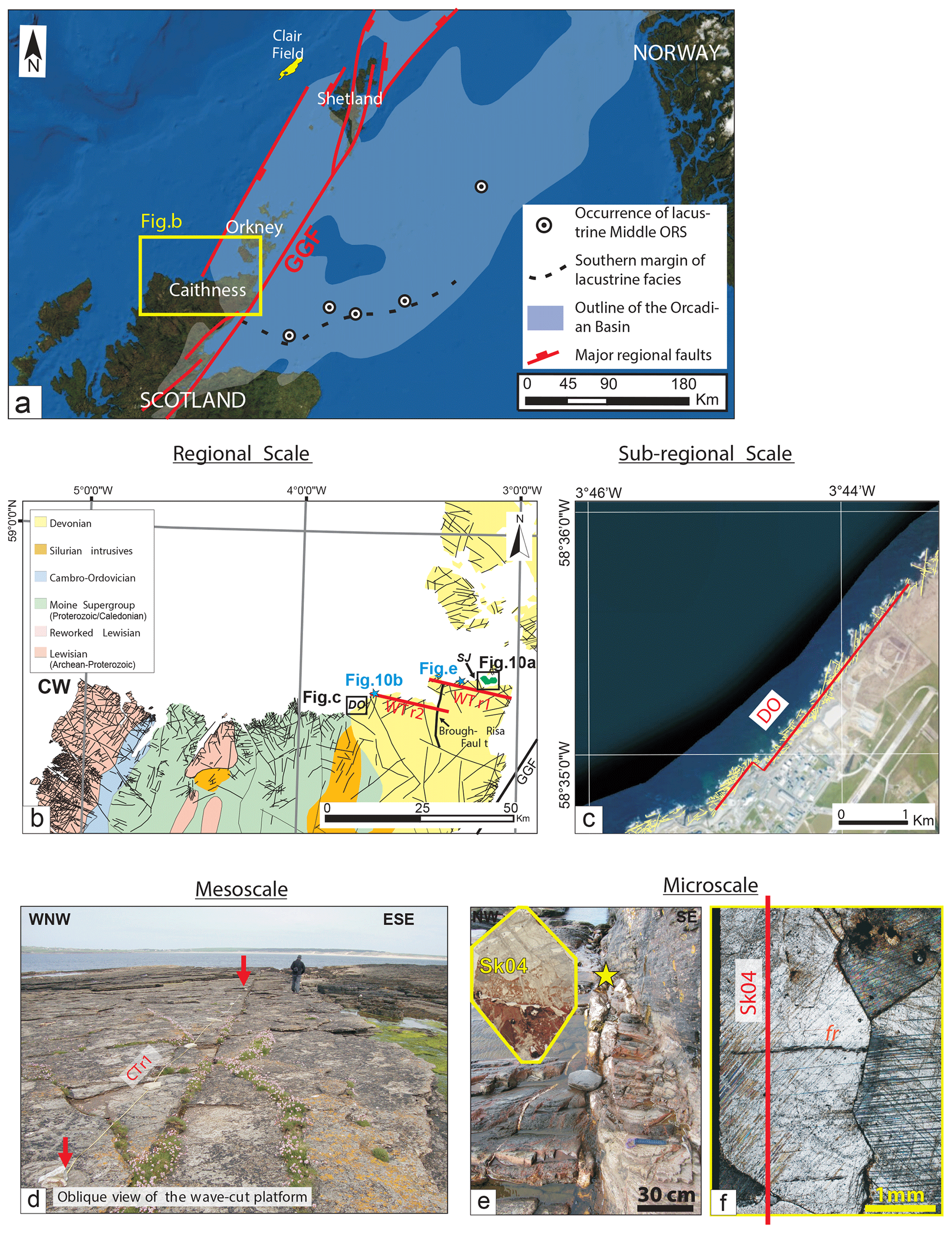
Figure 1 (a) Location map of the North Sea with the outline of the Orcadian Basin (light blue area). (b) Schematic geological map of northern Scotland showing the interpreted fault lineaments by Wilson et al. (2010) and the trace of the regional-scale transects (WTR1 and WTR2) and the location of the sub-regional transects (DO and SJ). (c) Example of Landsat aerial image showing the trace of the sub-regional-scale transect at Dounreay (DO). (d) Oblique view of the platform at Castletown. The metre ruler shows the trace of the transect CTr1 (mesoscale). (e) Outcrop photograph of the NE–SW fault zone where the sample for the thin section SK04 was collected (yellow star). (f) Thin-section photograph (top) with an example of one of the microphotographs showing one fracture. The trace of the scanline is shown by a continuous red line. CW: Cape Wrath; GGF: Great Glen Fault; fr: fracture; SK: Skarfskerry.

Recent fieldwork has shown that the onshore Devonian sedimentary rocks of the Orcadian Basin in Caithness host significant localized zones of fracturing, faulting and some folding on all scales. Field and microstructural analyses reveal three regionally recognized groups (sets) of structures based on orientation, kinematics and infill (Dichiarante et al., 2016, 2020; Dichiarante, 2017). In summary, these are as follows:

•  

  Group 1 faults trend mainly N–S and NW–SE and display predominantly sinistral strike-slip to dip-slip extensional movements. They form the dominant structures in the eastern regions of Caithness closest to the offshore trace of the Great Glen Fault (GGF) (Fig. 1a–b). Deformation bands, gouges and breccias associated with these faults display little or no mineralization or veining. It is suggested that these structures are related to Devonian ENE–WSW transtension associated with sinistral shear along the Great Glen Fault during formation of the Orcadian and proto-West Orkney basins (Wilson et al., 2010; Dichiarante et al., 2020a).

•  

  Group 2 structures are closely associated systems of metre- to kilometre-scale N–S-trending folds and thrusts related to a highly heterogeneous regional inversion event recognized locally throughout Caithness. Once again, fault rocks associated with these structures display little or no mineralization or veining. Group 2 features are likely due to late Carboniferous–early Permian E–W shortening related to dextral reactivation of the Great Glen Fault (Coward et al., 1989; Seranne, 1992; Dichiarante et al., 2020a).

•  

  Group 3 structures are the dominant fracture sets seen in the main coastal section west of St John's Point (SJ in Fig. 1b). They comprise dextral oblique NE–SW-trending faults and sinistral E–W trending faults with widespread syn-deformational low-temperature hydrothermal carbonate mineralization (± base metal sulfides and bitumen) both along faults and in associated mineral veins (Dichiarante et al., 2016). Hydrocarbons are widespread in fractures in small volumes and are locally sourced from organic-rich fish beds within the Devonian sequences of the Orcadian Basin (Parnell, 1985; Marshall et al., 1985). Re–Os model ages of syn-deformational fault-hosted pyrite in Caithness yield Permian ages (ca. 267 Ma; Dichiarante et al., 2016). This is consistent with the field observation that Group 3 deformation fractures and mineralization are synchronous with the emplacement of ENE-trending lamprophyre dikes east of Thurso (ca. 268–249 Ma based on K–Ar dating; Baxter and Mitchell, 1984). Stress inversion of fault slickenline data associated with the carbonate–pyrite–bitumen mineralization implies NW–SE regional rifting (Dichiarante et al., 2016), an episode also recognized farther west in the Caledonian basement of Sutherland (Wilson et al., 2010). Thus from St John's Point to Cape Wrath (CW in Fig. 1b), Permian-age faults are the dominant brittle structures developed along the north coast of Scotland, forming part of a regional-scale North Coast Transfer Zone translating extension from the offshore West Orkney Basin westwards into the North Minch Basin (see Dichiarante et al., 2016, 2020).

2.2 Group 3 structures – analogue for Clair reservoir

The Group 3 structures are the only set widely associated with syn-faulting mineralization and bitumen and have therefore clearly acted as fluid channel ways in the past. There is also good evidence for the preservation of open fractures and vuggy cavities consistent with these fractures continuing to be good potential fluid-flow pathways at the present day. No such features are associated with Group 1 or 2 structures. Most of the Group 3 fractures measured during the onshore study in the Orcadian Basin in Caithness are partially to completely filled with fault rocks, minerals or bitumen; a range of filling morphologies are preserved, which have been described by Dichiarante et al. (2016, 2020) (Fig. 2a–e). It is reasonable to assume that wholly bitumen-filled fractures can be viewed as being equivalent to open fractures in a sub-surface reservoir (Fig. 2a, b), whilst other veins may be completely filled with minerals/fault rock (lacking bitumen) or partially filled with hydrocarbon held in vuggy cavities (Fig. 2c), fractured mineral fills (Fig. 2) and/or porous sediment fills (Fig. 2e). There are many examples of partly or fully open fractures in the surface coastal exposures of the Orcadian Basin, but it is difficult to prove whether or not surface weathering and seawater washing of coastal outcrops have removed pre-existing fracture fills. This is supported by the observation that fracture-hosted bitumen fills are most widely preserved in recently exposed quarry or excavation sites inland (see Dichiarante et al., 2016). These authors presented textural evidence showing that fracture-hosted calcite, sulfides and oil fills are broadly contemporaneous. They suggest that open vugs and fractures are almost certainly only preserved due to hydrocarbon flooding, which shuts down the further precipitation of carbonate and sulfide in open or partially open fractures/veins (e.g. Fig. 2b–e).

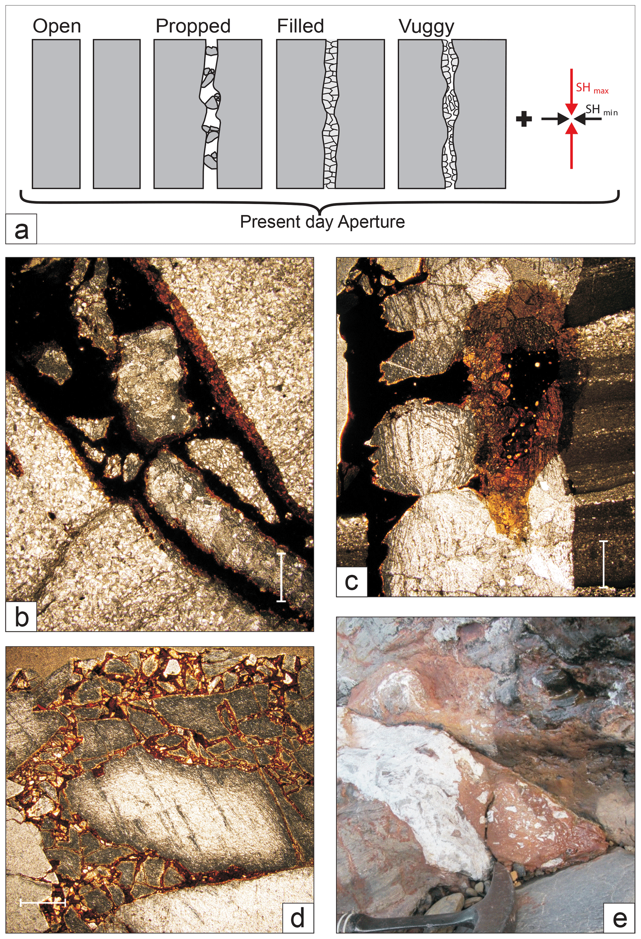
Figure 2 (a) Diagram summarizing how the aperture of a fracture is related to its morphology, its fill and the general influence of imposed stress. (b–e) Different fracture aperture and fill types associated with oil in the Orcadian Basin. (b) Photomicrograph of open fissure with oil fill and wall rock fragments, Thurso Bay foreshore; (c) photomicrograph of partial calcite fill with vuggy oil fill, Dounreay; (d) photomicrograph of oil-filled brecciated calcite in dilational jog, Dounreay; (e) Outcrop photo of calcite and red sandstone fill of inferred Permian age, Skarfskerry foreshore (see Fig. 1). All thin sections are taken in plane-polarized light, with scale bar = 1 mm.

Previous works, for example Barr et al. (2007), suggested that outcrops in the Orcadian Basin show similar features to the Clair field; in particular, they highlighted similar faults, open fractures, granulation seams, cemented fractures and in particular linear zones of fracturing as equivalent to linear zones of disaggregated core in the sub-surface. Our observations from the Clair field cores reveal similar associations between fractures filled, or partially filled, with similar hydrothermal minerals, younger porous sediment and hydrocarbons (see example in the data file in the Supplement, extracted from Dichiarante, 2017). This suggests that, despite differences in source rocks (local Devonian onshore versus more distant Jurassic offshore), the Orcadian Basin Group 3 fracture fills and apertures are a good analogue for the fractured rocks of the Clair Group. Barr et al. (2007) noted the presence of dispersed joints, in outcrops, which they attributed to exhumation features being much rarer in cores. In this study, we carried out fracture attribute analyses in areas where Group 3 structures predominate, or at locations where there is good field evidence that pre-existing Group 1 faults have undergone significant later reactivation synchronous with Group 3 age deformation (Dichiarante et al., 2020a). We did not include obvious early (Group 1 and 2) or late jointing in our fracture datasets.

Downie (1998) reported that sandstones of the middle ORS in the North Sea have poor reservoir quality due to widespread cementation comprised of calcite, dolomite, quartz overgrowths and clay minerals. This author also reported open fractures in all discoveries in “tight-matrix” sandstones in the Orcadian Basin (the Buchan, Stirling and West Brae fields) and that these features are present in the Clair field. He also referred to the presence of fracture-fill cements which are similar to the Group 3 structures of the Orcadian Basin. With reference to the three criteria for an analogue to be considered appropriate, as recently suggested by Ukar et al. (2019), (1) the Orcadian Basin outcrops show a similar structural setting and lithofacies, (2) the sandstone host rocks were in a similar state of diagenesis during the deformation and (3) the fracture cements show similar textures and formed under similar conditions to the producing structures in the Clair field. Thus, the Group 3 structures of the Orcadian Basin clearly formed in the sub-surface, and we argue that they are the best direct analogue for the oil-bearing fracture systems that occur in the Clair Group reservoir.

3 Methodology

3.1 Sampling of fractures and fracture network attributes

The most common data acquisition methodologies use (i) scanlines (or transects), (ii) window sampling, (iii) circular scanline windows and (iv) box counting (Fig. 3), which collectively provide access to different attributes as shown in Table 1. Scanlines (1D method) allow a relatively simple characterization of individual fracture sizes and spacing and act as a good proxy for the borehole data that typically serve as starting points for building reservoir models (Priest and Hudson, 1981; Baecher, 1983; Gillespie et al., 1993; McCaffrey and Johnston, 1996; Knott et al., 1996; Ortega and Marrett, 2000; Ortega et al., 2006; Bonnet et al., 2001; Odling et al., 1999). Window sampling and circular scanline windows (both 2D methods) provide further information on the spatial relationships within the fractured system (Mauldon, 1994; Mauldon et al., 2001; Rohrbaugh et al., 2002; Manzocchi, 2002; Zeeb et al., 2013; Watkins et al., 2015; Sanderson and Nixon, 2015; Rizzo et al., 2017) and importantly provide access to connectivity estimates for the fracture array, which is a key input when modelling fluid flow.

Table 1 Basic parameters, definitions and equations provided by 1D and 2D methods (Zeeb et al., 2013, modified).

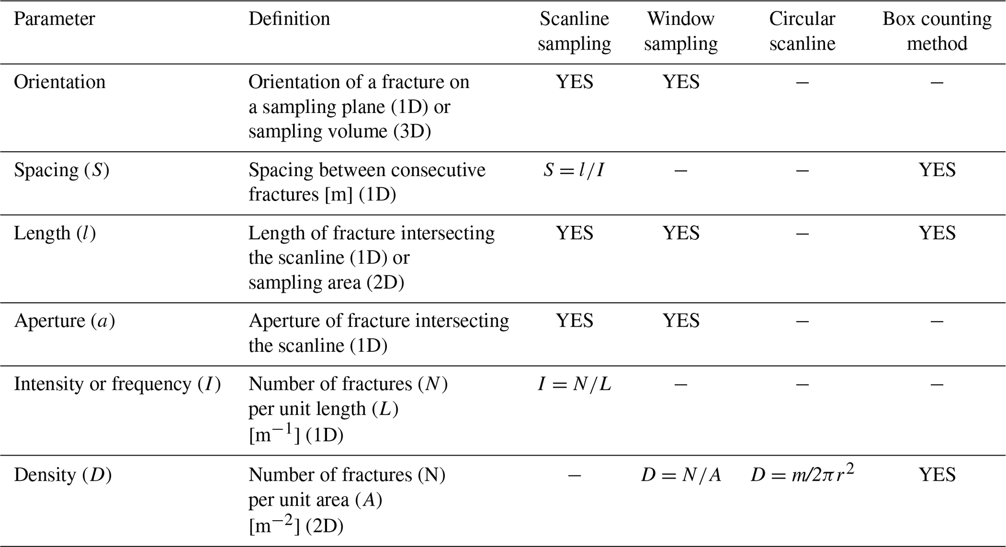
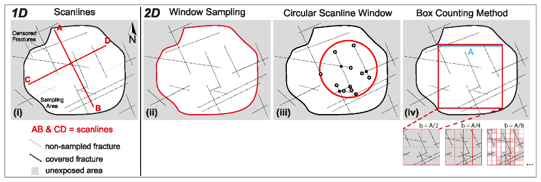
Figure 3 Synthesis of 1D and 2D methodologies for estimating fracture attributes: (i) scanline sampling (or transect), (ii) window sampling, (iii) circular scanline window and (iv) box counting method (modified after Zeeb et al., 2013). A: box counting size.

In this study, fracture orientations, trace lengths and apertures, together with composition and texture of fracture infills and fracture terminations, for all Group 3 structures were recorded. The start and end point of each transect was recorded using a hand-held GPS unit. Most fractures in the Orcadian Basin are filled with minerals (calcite or pyrite) or, locally, oil, and, following Ortega et al. (2006), the apertures measured in this study are the orthogonal distance between the fracture walls and include the fill, i.e. the “kinematic aperture”. Most Group 3 fracture sets are made up of fracture meshes (sensu Hill, 1977; Sibson, 1996) formed by closely interlinked sets of contemporaneous shear fractures and tensile veins (Dichiarante et al., 2016, 2020). Thus, in each sample, all fractures considered to belong to an individual fracture set (in this case Group 3) were included in the analysis regardless of opening mode. Thus in our view it is not possible to separate brittle structures into separate sets of simple tensile and shear fractures. This practical approach ensures comparability with sub-surface structures in Clair cover sequences and related fractured basement studies where similar interlinked mesh systems are dominant (see McCaffrey et al., 2020). One reason for the development of such mesh networks is that many Group 3 structures reactivate earlier (Group 1 and 2) brittle structures and therefore display a variety of hybrid opening modes (Dempsey et al., 2014).

When it was not possible to measure the transect orthogonally to the main fault because of outcrop exposure limitations (e.g. at the sub-regional scale), the measured attributes were adjusted using the Terzaghi correction (Terzaghi, 1965). To more precisely measure the aperture attributes, an engineering feeler gauge in conjunction with a hand lens (10⁻⁵ to 10⁻⁴ m) was used in the field in order to ensure a larger range of recorded apertures, thereby reducing censoring effects.

To extend the analysis to other scales, the above-mentioned scanline method was adapted and applied to both aerial photographs (regional scale) to quantify trace length and the thin section (microscale) to quantify trace length and aperture. Fracture lengths mapped as continuous at regional scale are likely to comprise segments which may not be resolvable at the scale of observation. However in terms of fluid flow, segmented faults may be connected as single structures at depth, so our lineaments may represent an interconnected length in the sense of Olson (2003).

3.1.1 Fracture intensity/frequency plots (1D)

The fracture intensity/frequency distribution for 1D datasets can be visualized by plotting sorted attribute values (e.g. fracture length) versus cumulative frequency. This enables assessment of the distribution, spatial and scaling properties of the fracture sample (i.e. the ratio of short to long fractures for a given sample line length). Fracture attribute distributions are thought to display three main types of statistical distribution (Fig. 4, Bonnet et al., 2001; Gillespie et al., 1993; Zeeb et al., 2013): (a) exponential, random or Poisson distributions are characteristic of a system with one randomized variable (Gillespie et al., 1993); (b) log-normal distributions are generally produced by systems with a characteristic length scale where mechanical stratigraphic boundaries control joint spacing for example (Narr, 1991 and Olson, 2007); and (c) power-law distributions lack a characteristic length scale in the fracture growth process (Zeeb et al., 2013), and the data exhibit scale-invariant fractal geometries (Fig. 4c bottom). For a power-law distribution, the relative number of small versus large elements remains the same at all scales between the upper and lower fractal limits (Barton, 1995). Ideally, the best fit in a power-law distribution should be consistent over a length scale of several orders of magnitude (Walsh and Watterson, 1993; McCaffrey and Johnston, 1996). Limits to the fractal behaviour can be related to both spatial and temporal influence, for example lithological boundaries across which fracture characteristics change, changes in stress orientation or diagenetic effects (Hooker et al., 2014). However, it is generally accepted that power-law distributions and fractal geometry provide a widely applicable descriptive tool for fracture size attributes such as aperture and length (e.g. Bonnet et al., 2001; Olson, 2007; Hooker et al., 2014; McCaffrey et al., 2020).

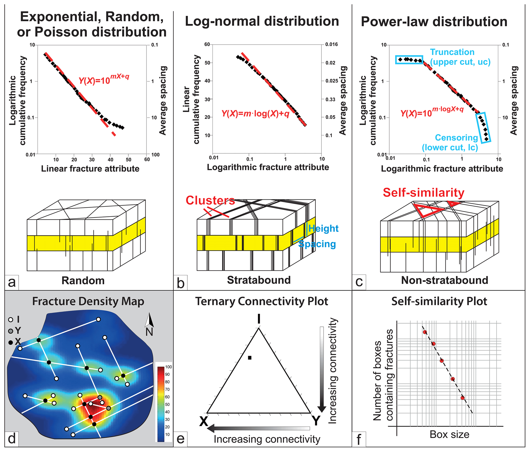
Figure 4 Population distribution plots for (a) exponential (linear–logarithmic axes), (b) log-normal (logarithmic–linear axes) and (c) power-law (logarithmic–logarithmic axes) distributions with relative best-fit equations (top) and sketch of physical meaning (bottom). Note that Hooker et al. (2013) proposed an alternative 4-fold classification scheme for bed boundedness. On the distribution plots, datasets are shown as black diamonds and typical best fits are shown as dashed red lines. (d) Examples of density maps showing higher connectivity where Y and X nodes occur, (e) ternary plots showing that the overall system shown in Fig. 4d is isolated and (f) self-similarity plot method from Fig. 3 (iv).

Fracture sampling issues (e.g. censoring and truncation in Fig. 4c) are commonly encountered and can result in difficulty in ascribing the best-fit distribution. For instance, when long fractures are incompletely sampled (e.g. censoring in Fig. 4c), it is difficult to determine between log-normal and power-law fits to distributions. These sampling issues (due to resolution effects) may mean that, while a log-normal distribution is the best fit to a dataset, a power-law distribution can also show a good fit (Corral and González, 2019) and may be preferred because of its greater physical significance and practical applicability (Bonnet et al., 2001). These assumptions need to be examined closely in any analysis of scaling (see Clauset et al., 2009), and power-law behaviour should not be assumed. The maximum-likelihood estimator (MLE) is a statistical technique that determines which distribution model is most likely to describe the data, and it returns governing parameters of the fitting equations (see data file in the Supplement). The Kolmogorov–Smirnov (KS) test is then used to evaluate the difference between the data and synthetic data generated using the governing parameter derived from the MLE (Clauset et al., 2009). We use these statistical methods and adapted the methodology proposed by Rizzo et al. (2017) and used in FracPaQ (Healy et al., 2017) to calculate the MLE on progressively truncated populations for power-law, exponential and log-normal distributions.

3.1.2 2D topology analysis

Whilst 1D analyses provide information about fractures as single entities and their distribution per unit length of sample, 2D analyses measure fracture network properties and provide estimates of fracture connectivity and self-similarity. The 2D analysis used here was carried out on fractures at mesoscale using outcrop pavement photographs and at a larger scale using offshore bathymetric data. Circular scanline windows and box counting methods were performed using the CorelDRAW Graphics Suite™, ArcGis™ and MATLAB™ to produce small-scale fracture density maps (Fig. 4d), ternary plots of connection types (Fig. 4e) and box counting dimension (Fig. 4f). To understand fracture topology, we follow Sanderson and Nixon (2015) in considering that fracture arrays are typically composed of nodes and branches. Nodes are points where a fracture terminates (I type), abuts against another fracture (Y type) or intersects another fracture (X type), and branches are the portions of a fracture confined between two nodes. These branches are defined as I–I type (isolated) if delimited by two I nodes, I–C type (singly connected) if delimited by an I node and Y or X node, and C–C type (multiply connected) if delimited by Y and X nodes.

The number of branches and nodes for a given fracture network is strictly related, meaning that, by knowing one of the two elements for the fracture network, it is possible to quantify all its components. N_I,N_Y and N_X can be defined as the number of I-, Y- and X-type nodes, and P_I, P_Y and P_X their relative proportions. Once the number of nodes and/or branches making up a fracture array is known, the fracture trace connectivity can be visualized using the ternary plot of the component proportions (see e.g. Fig. 4e) or can be quantified by calculating the number of connections existing in the 2D map. In general, X- and Y-type nodes provide respectively 4 and 3 times more connectivity than I-type nodes (Nixon, 2013). This forms the basis for creating 2D density maps (see Fig. 4d). An array dominated by I nodes is isolated, while arrays dominated by Y- and X-type nodes are increasingly more connected. Connectivity can be quantified by measuring the number of connections per line $n_{\mathrm{C}/\phantom{\mathrm{CL}}\mathrm{L}}$ and the number of connections per branch $n_{\mathrm{C}/\phantom{\mathrm{CB}}\mathrm{B}}$ (see Sanderson and Nixon, 2015 for details).

4 Locations and orientation data from the 1D scanlines

In the present study, 1D scanlines were performed at different scales in the Caithness area, resulting in datasets of regional (kilometre scale, Fig. 1b), sub-regional (10² m to metre scale, Fig. 1c), meso- (metre to centimetre scale, Fig. 1d) and microscales (micron scale, Fig. 1e and f).

4.1 Regional and sub-regional scale

Scanline data have been collected at a regional scale (kilometre scale) using a tectonic lineament interpretation map created by Wilson et al. (2010). In their study, the lineament analysis was conducted at 1:100 k scale extending from Lewisian basement outcrops in western Sutherland eastwards into the Devonian rocks of Caithness (Fig. 1b). We performed two scanlines (WTr1 and WTr2) trending orthogonally to the Brough–Risa Fault, the major N–S-trending basin-scale fault in Caithness (Fig. 1b; Dichiarante et al., 2016). Scanline WTr1 intersects mainly NE–SW- and NW–SE-trending lineaments, while scanline WTr2 intersects mainly N–S- and a few NE–SW-trending lineaments (Fig. 1a). Although datasets with few data points generally give poorly defined distributions on graphical presentations, it will be shown that the data from these two transects are of value in the multiscale approach adopted here.

At the sub-regional scale, scanlines have been performed on lineament maps produced from Google Earth satellite images at 1:1 k scale (pixel resolution: ca. 10 m²?). These datasets are limited to well-exposed wave-cut platforms on the coast because the flat topography and thick cover of drift have obscured the structures inland. The interpreted lineaments from the images were verified during fieldwork as being faults (large to mesoscale) and joints and not anthropogenic features. The narrow width of the platform limits the analysis to only one scanline at each locality (DO at Dounreay, SJ at St John's Point; see Fig. 1c). We estimate that we would have recorded 10–20 % of the total number sampled at these localities if the transect line had followed the sub-regional trend rather than the outcrop extent. Fracture spacing measurements were corrected using the Terzaghi correction (see dashed red and blue lines in the rose diagrams in Fig. 5b–c).

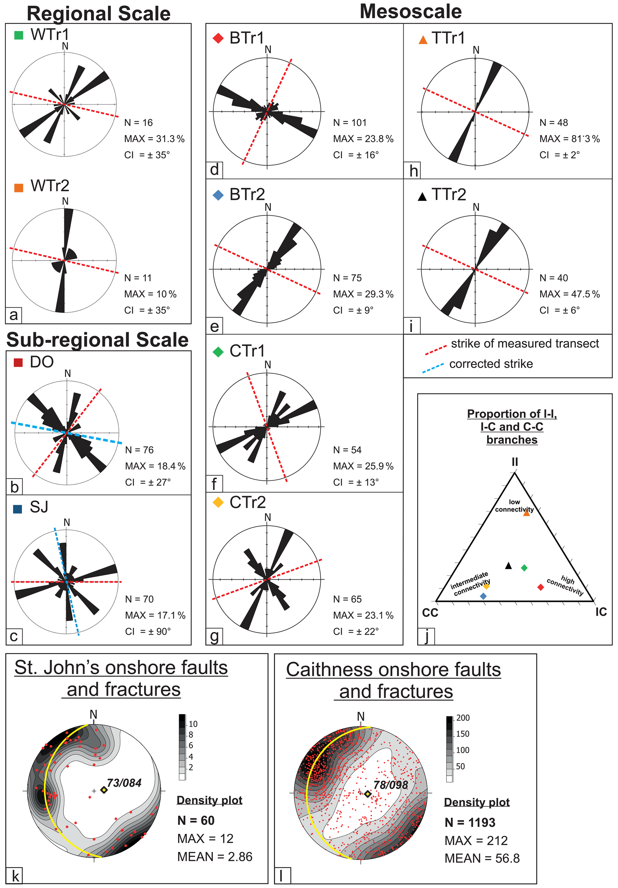
Figure 5 Rose diagrams of fracture orientation data for the transects at (a) regional scale, (b, c) sub-regional scale and (d, i) mesoscale. Locations are given in Fig. 1. Note that the mesoscale transect trend is corrected to be the same as the transects at sub-regional scale (dashed blue lines in rose diagrams). (j) Ternary plot providing an estimation of the different type of fracture branches intersecting each transect. N: number of fractures; MAX: maximum; CI: 95 % confidence interval. Lower-hemisphere equal-area projections of measured offshore data at (k) St John's Point and (l) Caithness. Note that the best fit of fault and fracture data collected onshore at St John's Point (yellow diamond in the top stereonet) is consistent with the best fit of fault and fractures data collected in Caithness (yellow diamond in the bottom stereonet; Dichiarante, 2017). MAX: maximum density; MEAN: mean density.

The scanline at Dounreay (DO) is NE–SW trending and intersects mainly NW–SE- and NNE–SSW-trending lineaments, with a subset of NE–SW-trending lineaments (Fig. 5b). The scanline at St John's Point (SJ) intercepts mainly ENE–WSW-trending lineaments with subsets of N–S- and NW–SE-trending lineaments (Fig. 5c).

4.2 Mesoscale outcrops

Fracture data along six mesoscale scanlines were collected at three field localities where there is very good exposure: Brims Ness (BTr1, BTr2; Fig. 5d, e), Castletown (CTr1, CTr2; Fig. 5f, g) and Thurso (TTr1, TTr2; Fig. 5h, i). In each outcrop, the position, direction and length of the scanlines were chosen with reference to the trend of the basin-scale master faults in each area (e.g. ENE-WSW at Castletown and NNE–SSW at Thurso and Brims Ness; Fig. 5d–i). At Castletown and Brims Ness, two scanlines were carried out to record the full range of fracture orientations: one parallel and one perpendicular to the master fault set. Scanlines at Thurso differ from the others because they are both measured parallel and next to a fault zone, resulting in higher values of fracture intensity (see TTr1 and TTr2 in Table 2). These scanlines are also shorter (< 4 m) and record exclusively thin veins. Each locality is characterized by one (e.g. Thurso) or more fracture sets (e.g. Castletown and Brims Ness). Where two sets of fractures are present, they mutually cross-cut each other, which enabled us to infer that they were active during the same geological event; hence they are analysed here as a single population (Dichiarante, 2017).

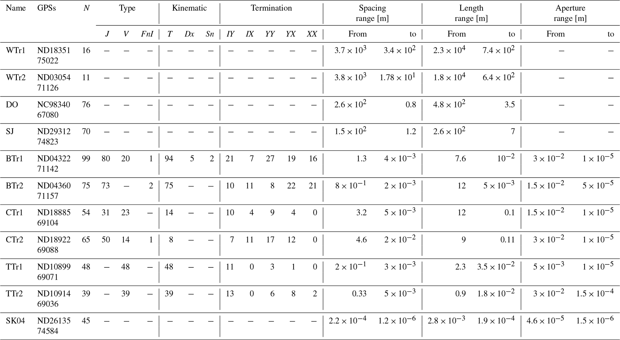
Table 2 Transect data. GPSs: GPS position of the starting point; N: total number of sampled fractures; J: joint; V: vein; FnI: fracture without infill; T: tensile; Dx: dextral; Sn: sinistral; IY and IX: ”singly connected” branches, delimited by one I node and one Y or X node; YY, YX and XX: ”multiply connected” branches, delimited by two Y or X nodes or one Y and one X node.

Additionally, for each scanline, fracture termination type, kinematics and type of fractures were recorded (Table 2). Although fracture terminations are more usefully assessed in a 2D analysis, we recorded the nature of fracture branch terminations for each structure intersecting the transect line. These data are reported using a ternary plot (Fig. 5j) which shows that there is no dominant fracture termination type. In general, the transects show intermediate to high connectivity, except for scanline TTr1, which shows a more isolated pattern.

An orientation analysis of fracture intersection has been carried out for onshore fault and fracture data at St John's Point (Fig. 5k, Dichiarante, 2017), based on its proximity and geological similarity to the area covered by the bathymetric map which lies immediately offshore (see Sect. 7). A similar plot is also shown for all the fault and fracture data collected in Caithness (Fig. 5l, Dichiarante, 2017). Both datasets show consistent best-fit intersections that are sub-vertical to steeply plunging to the east, 73∕084 and 78∕098, respectively (yellow diamonds in the stereonet in Fig. 5k and l).

4.3 Microscale scanline

At microscales, one transect was performed on an oriented thin section taken from sample SK04 (inset in Fig. 1e, left). At the scale of a thin section, only samples from fault zones contain enough fractures to produce a statistically significant sample. We thus recognize that the results at this scale are representative of fracture intensities within fault zones and provide an upper limit relative to background. Our field observations ensured that the age of this fault was the same as the other Group 3 structures analysed at different scales. This fault rock was chosen as it is a typical example of a NE-trending fault with normal dextral oblique kinematics, filled with carbonate mineralization and red-stained (hematite) sandstone breccia of inferred Permian age (Fig. 1e; see also Fig. 2e). The oriented thin section was analysed under an optical microscope, and the spacing, aperture and lengths of microfractures were recorded. Photomicrographs were merged, and the scanline was measured orthogonally to the bounding NE–SW meso-fracture (Fig. 1f).

5 1D fracture population results

5.1 Fracture length, aperture and intensity/spacing results

MLE distribution fitting and KS tests were performed for all datasets and different types of distribution (exponential, log-normal and power law). The recorded range values of trace length and aperture (or vein width) for each of datasets are shown in Table 2. In Tables 3 and 4 in the data file in the Supplement, we report the MLE distribution fitting results for both non-truncated (exponential, log-normal and power-law distributions) and truncated (power-law distribution) populations for trace length and aperture, respectively.

Length population datasets yielded values, rounded to the nearest order of magnitude, centred at ca. 10 m for the sub-regional scale, 10⁻¹ m at mesoscale and 10⁻⁴ m at microscale (Fig. 6a). Aperture populations are centred between ca. 10⁻³ m for the mesoscale dataset and ca. 10⁻⁵ m for the microscale dataset (Fig. 6).

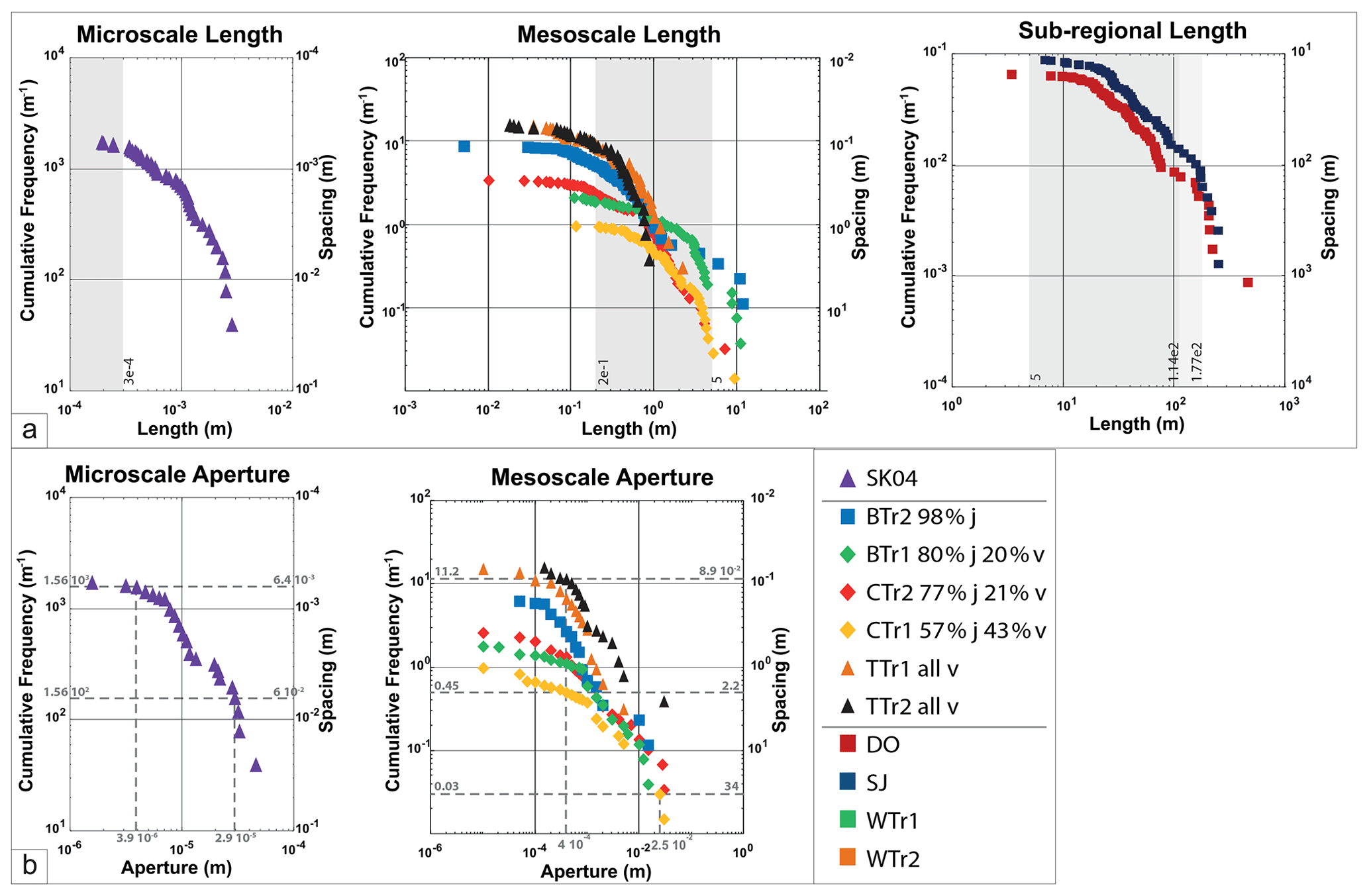
Figure 6 Cumulative distribution plots of (a) fracture and fault trace length for transects at (left) microscale, (centre) mesoscale and (right) sub-regional scale and (b) kinematic aperture for transects at (left) microscale and (right) mesoscale. On the plots reported stratigraphic layer thicknesses are shown as grey boxes. The Ham–Skarfskerry Subgroup (177 m) and the Latheron Subgroup (114 m) from Andrews et al. (2016) are shown on the sub-regional-scale plot. The Lower Stromness Flagstone (5 m) on the sub-regional-scale and mesoscale plots. On the mesoscale plot the average thickness of beds (ca. 20 cm) is also plotted. On the microscale plot, the thickness of individual laminae (ca. 0.3 mm) is shown. Dashed lines and number refer to values discussed in text.

The plots in Fig. 6 give an insight into the relationship between cumulative frequency/intensity (inverse spacing) and length or aperture. For example, at the mesoscale (Fig. 6b right), the intensity of fractures with > 25 mm aperture is about 0.3 m⁻¹, corresponding to a 34 m spacing. Similarly, the intensity of fractures with > 0.4 mm aperture is between 0.45 and 11.2 m⁻¹, corresponding to 8.9 cm to 2.2 m spacing, respectively. At microscales (Fig. 6b left), the intensity of fractures with $\mathit{>}\mathrm{2.9}\times {\mathrm{10}}^{-\mathrm{5}}$ m aperture is about 155.51 m⁻¹, corresponding to 6 mm spacing, whilst the intensity of fractures with $\mathit{>}\mathrm{3.9}\times {\mathrm{10}}^{-\mathrm{6}}$ m aperture is about 1555 m⁻¹, corresponding to a 0.64 mm spacing. These spacing values do not take into account any systematic spatial arrangement. Using the Marrett et al. (2018) spatial correlation analysis on our 1D fracture samples, we see fractal clustering with 0.02–0.2 m spaces twice as likely compared to a random distribution at Castletown, Thurso and Brims Ness. These are arranged in 1–3 m wide clusters spaced at 1–20 m. At larger scale, Dounreay shows cluster widths of 650 m spaced with 5 km intervals. In contrast, St John's Point shows anti-clustered (regularly spaced) fractures at ca. 2 m (see plots in the data file in the Supplement).

To examine the possible influence of mechanical stratigraphy on fracture scaling across the Orcadian Basin in Caithness, we indicate, on the fracture size plots, selected sedimentary unit thickness values reported in previous studies (Fig. 6). These include sedimentary laminae thickness (0.3 mm) at microscale, bedding-range thicknesses of the Lower Stromness Flagstone Formation (20 cm to 5 m) at mesoscale, and thicknesses of the Ham–Skarfskerry and Latheron subgroups at sub-regional scales (data from Andrews et al., 2016). Also, the approximate boundary between faults that can be imagined in seismic reflection images and smaller-scale structures is shown in Fig. 8 (yellow arrows) based on well-known empirical displacement–length relationships (a 10 m displacement corresponding to a length of ca. 100 m, following Kim and Sanderson, 2005).

Analysis of uncertainties: validity of data populations and reliability of best-fit distributions

In any statistical analysis, the sampled population should be large enough to give a statistically acceptable representation of the population and to properly determine the distribution type and its parameters (Bonnet et al., 2001). The sample sets are statistically valid for most samples after the first 20 measurements (grey area in Fig. 7) because the cumulative fracture intensity of the population data and its standard deviation (black and green curves, respectively) become reasonably stable. The uncertainty in the cumulative fracture intensity reduces progressively towards the end of the scanline.

Figure 7 Fracture intensity and standard deviation as a function of fracture number for (a) sub-regional-scale, (b) mesoscale and (c) microscale transects. Fracture intensity is unstable for a relatively small number (< 20) of detected fractures (grey area).

6 The scalability of fracture attributes

6.1 Slope determination – MLE approach

The complete (non-truncated) populations show that a log-normal distribution best describes the data as they show consistently high-percentage fitting values. However, the choice of the best-fit distribution should not be based on the complete population because the distribution tails (corresponding to the largest and smallest size fractures) are biased (see also data file in the Supplement). We therefore also investigated progressively truncated populations in order to validate the hypothesis. The fitting results for complete log-normal and truncated power-law datasets are generally similar (see data files in the Supplement), suggesting that either type of distribution can successfully describe the size attribute data.

6.2 Multiscale analysis

Trace length distribution data from all transects have been normalized using sample line length (cf. Marrett et al., 1999) and are displayed together on a single population plot (Fig. 8a), which enables us to assess scaling over 8 orders of magnitude (10⁻⁴ to 10⁴). The grey region in Fig. 8a shows that the multiscale data can be described by a power-law distribution with the overall scaling coefficient close to a slope of −1 centred on a 1 m length fracture with a 1 m spacing. This power-law distribution implies fractal or self-similar behaviour of the length parameter over 8 orders of magnitude, which effectively means that the fracture array maintains the same statistical properties of intensity and length at all scales assessed here.

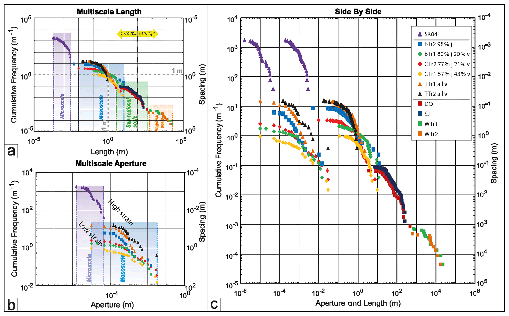
Figure 8 Cumulative frequency plots of (a) fracture length and (b) fracture aperture. (c) Side-by-side population distribution plots of length (right side of the plot) and aperture (left side of the plot). Note that the distance between the datasets at different localities (down to mesoscale) represents the relationship in terms of order magnitude between aperture and length. Information about thickness of Devonian rock are displayed as dashed lines (a). j: joints; v: veins.

The aperture datasets collected in the meso- and microscale transects are also shown on a single population plot (Fig. 8b) and show evidence for an overall power-law scaling over 4 orders of magnitude (10⁻⁶ to 10⁻²), also with a slope of −1. However, the best-fit line is centred on a 1 mm wide fracture with a 1 m spacing. This overall slope is indicative of a fractal distribution or self-similar behaviour of the aperture parameter over 4 orders of magnitude, which means that the fracture array maintains the same relationship between intensity and aperture at all scales assessed here.

In order to assess whether stratigraphic units influenced the fracture scaling, the estimated overall thickness of the Devonian rocks in Caithness by Donovan (1975) and the smallest-scale bedding planes of ca. 10⁻⁴ m that were observed in thin section are shown in Fig. 8a (dashed red lines). These limits approximately span the range of fracture lengths recorded, and the absence of obvious slope changes between the limits suggests that stratigraphic element have not played a role in determining the fracture scaling.

6.3 Length–aperture correlations

Trace length and aperture or vein width data are plotted side by side to illustrate the positive correlation between these attributes over 4 orders of magnitude (Fig. 8c). A linear scale length–aperture scatter plot in Fig. 9a shows that the data are clustered towards the origin, reflecting the greater frequency of smaller fractures expected for a power-law distribution (Vermilye and Scholz, 1995; Olson, 2003; Schultz et al., 2008). The plot of logarithmic length vs. logarithmic aperture in Fig. 9b shows two clusters of data which correspond to the mesoscale population (larger datasets in the centre of the figure) and the microscale population (bottom left dataset). Small-aperture mesoscale data are poorly resolved, plotting at either 0.01 or 0.05 mm due to the effect of using the thickness comparator in the field. On the distribution plots, this artefact is removed conventionally by only plotting the highest cumulative frequency for each aperture value. In contrast, however, on the aperture–length plot each individual data point of the cloud is statistically equally important, although this results in increased uncertainty at lower aperture values. The logarithmic plot for veins only (triangles in Fig. 9b), showing a clear positive power-law relationship between aperture and length, has less pronounced artefacts and permits an appraisal of the relationship between these two parameters. Line fitting methods suggest a slope of 0.65 or larger with a R² of 0.75 (red line in Fig. 9b) for all fracture data in this study. A comparison of veins (triangles) with other fractures including joints (grey dots in Fig. 9b) might further suggest that veins tend to be shorter for any given aperture.

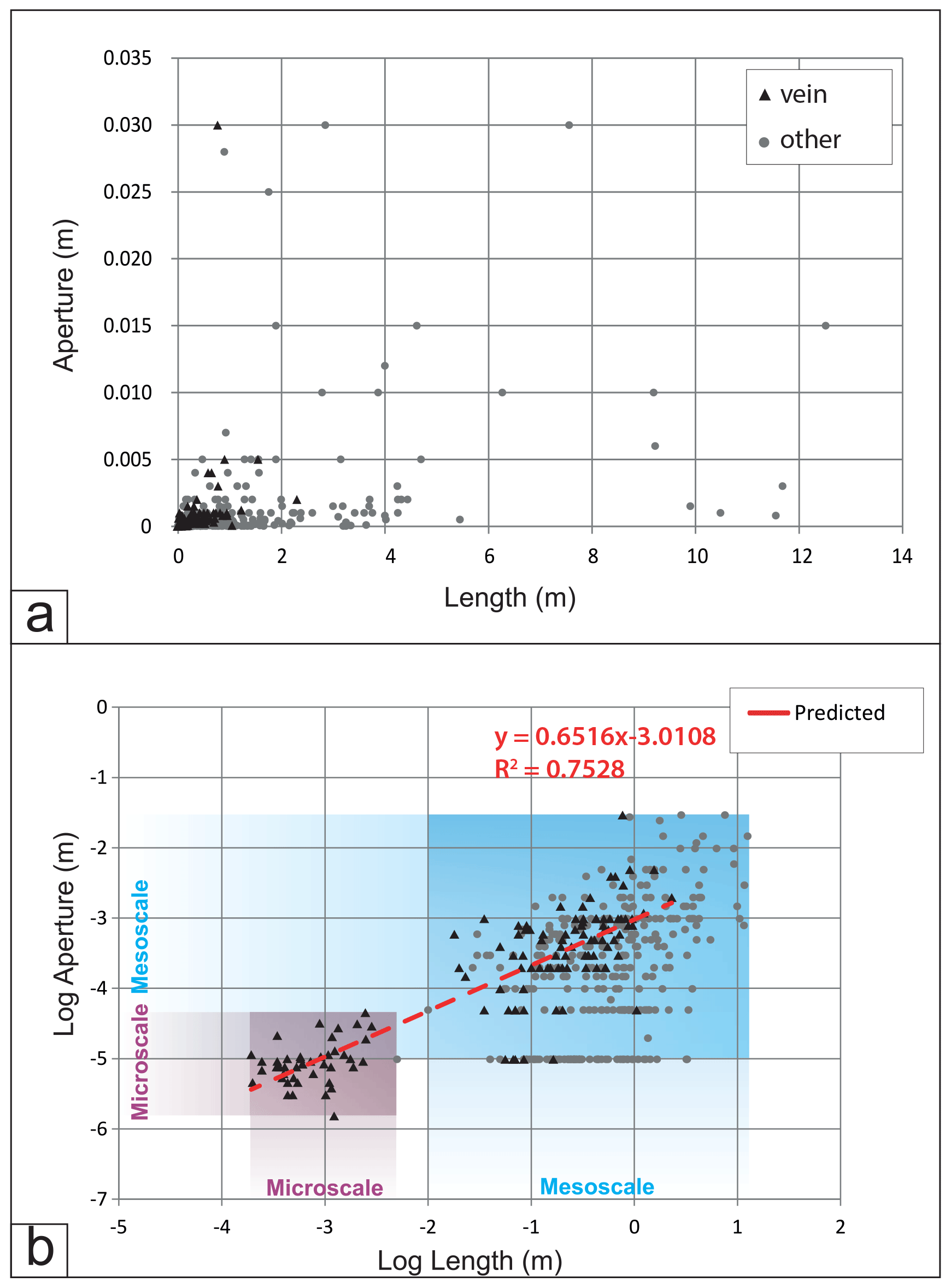
Figure 9 (a) Length–aperture scatter plot and (b) log of length vs. log of aperture for veins (triangles) and other structures (circle). Linear regression for veins on the logarithmic plot is shown (dashed red line).

7 2D population analysis

7.1 2D sampling locations

The 2D analysis was conducted at sub-regional scale on a bathymetric map from the near-offshore area (Fig. 10a) and at mesoscale using a photograph of a large rock pavement outcrop (Fig. 10b) to provide quantitative assessments of fracture connectivity and self-similarity. The offshore data provide access to a much larger area compared to onshore; however, the nature of the fractures themselves can only be constrained by extrapolation from adjacent onshore exposures. We chose to perform 2D analysis on these areas for two main reasons. First, both contain large numbers of fractures spread over a large plan view area and therefore were most likely to provide a statistically meaningful analysis using different 2D methods (e.g. circular scanline windows and box counting). Second, the difference in size between the two areas gives an insight into fracture scaling properties. The fracture interpretation of the bathymetric image enabled analysis of the fracture length distribution for comparison with the 1D results and a topological fracture network analysis of the fracture nodes.

Figure 10 (a) 2D analysis of bathymetric data from the area between St John's Point and Stroma Island with lineament interpretation and I, Y and X nodes; rose diagrams of lineaments; and ternary plot of node-type proportions. (b) 2D analysis of outcrop pavement photograph with lineament interpretation and I, Y and X nodes, and ternary plot of node-type proportions. MAX: maximum density.

The bathymetry map used for this study is a high-resolution multibeam dataset provided by MeyGen Ltd (IXsurvey Ltd, 2009) in the area between St John's Point and Stroma Island where the Devonian rocks are exposed on the seafloor, which has been washed clean by the action of strong water currents (Fig. 10a, raw image in data file in the Supplement). The largest structures in the bathymetry were interpreted by the data providers as faults and fractures. Moreover, the ENE-oriented structures have the same strike as minor faults and fractures observed on the coastal platform at St John's Point (and Stroma Island). The northernmost and longest lineament aligns well with a small bay where we observed intense faulting (and folding) related to mineralized, sinistral ENE-striking faults (classified as Group 3 structures). The N–S-oriented structures are most likely to be reactivated faults (Dichiarante, 2017).

A similar 2D analysis was carried out using a mesoscale photograph taken at Brims Ness (location in Fig. 1b and raw image in data file in the Supplement). Distortion effects were minimized by analysing a single photo taken orthogonally to the outcrop pavement and by conducting the analysis in a circular area to avoid edge distortions. These structures are thought to be associated with dextral reactivation of the Bridge of Forss Fault, and, based on their similar style, associated mineralization and kinematics are inferred to be the same age as the Group 3 structures dated as Permian by Dichiarante et al. (2016).

2D fracture patterns

Interpreted faults from the bathymetric data show ENE–WSW and NNW–SSE orientations. ENE–WSW-trending faults dominate in this region (see SJ rose diagram in Fig. 5a) and show corridor arrangements in the sense of Questiaux et al. (2010). The orientations of these faults are comparable to the two main fault sets seen onshore at locations such as St John's Point (Fig. 5c). NNW–SSE-trending faults are regularly spaced (100 to 200 m) in the central part of the area, while the ENE–WSW-trending faults are present across the entire survey. The latter set show two different spacing values: less than 100 m for the shorter structures and about 1000 m for larger structures.

The Brims Ness photo shows three different sets of fractures: N–S, NE–SW and WNW–ESE trending (Fig. 10b). The N–S- and NE–SW-trending structures form the majority of the fractures. Most fractures have straight traces and cross-cut each other. Three larger WNW–ESE- and NNE–NE-trending faults were detected. A single curved WNW–ESE-trending fault was also identified (Fig. 10b).

7.2 Fracture topology results and fracture connectivity

The bathymetric topology is comprised of 698 I, 123 Y and 117 X nodes (yellow, cyan and red squares in Fig. 10a, respectively), whilst the outcrop topology is composed of 916 I, 240 Y and 202 X nodes (yellow, cyan and red squares in Fig. 10b, respectively).

I-type nodes are regularly distributed in the area, while Y- and X-type nodes mainly occur in the central part of the bathymetry map, where longer ENE–WSW-trending faults occur (Fig. 10a). X- and Y-type nodes, which contribute most to connectivity of the 2D system, are mainly localized where the ENE–WSW-trending faults cross-cut NNW–SSE-trending structures.

The number of connections per line ($n_{\mathrm{C}/\phantom{\mathrm{CL}}\mathrm{L}}$) and number of connections per branches ($n_{\mathrm{C}/\phantom{\mathrm{CB}}\mathrm{B}}$) are respectively 1.18 and 1.1 for the bathymetry image, and 1.53 and 1.22 for the outcrop analysis (on a scale that ranges between 0 and ∞ for $n_{\mathrm{C}/\phantom{\mathrm{CL}}\mathrm{L}}$ and between 0 and 2 for $n_{\mathrm{C}/\phantom{\mathrm{CB}}\mathrm{B}}$). This indicates low overall connectivity for the fracture systems exposed in 2D. The $n_{\mathrm{C}/\phantom{\mathrm{CL}}\mathrm{L}}$ is also shown on a ternary I–Y–X plot (inset in the bottom left of Fig. 10a and b).

For the bathymetry dataset, the nodal density map shows that a large majority of nodes are aligned along a series of ENE–WSW-trending faults (Fig. 11a top). The density map shows that Y and X nodes are mainly associated with NNW–SSE-trending faults and are responsible for producing most of the connectivity of the system (Fig. 11a bottom). For the pavement, the nodal density is higher at intersection between N–S-trending and NE–SW-trending fractures and where these fractures are longer (Fig. 11b).

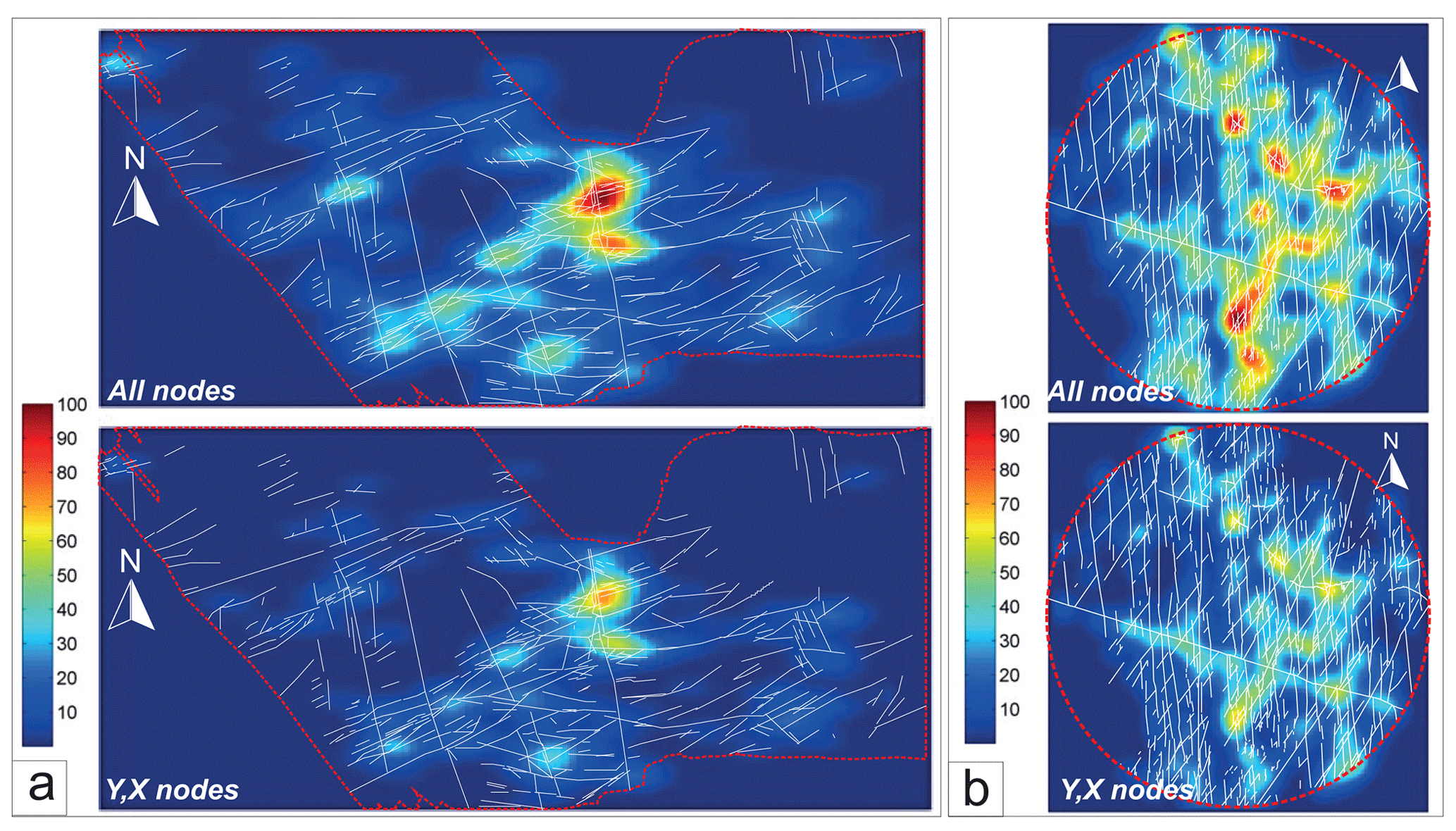
Figure 11 Lineament and density maps of nodes for (a) the bathymetry fault network and (b) the fault network in pavement. All-node density map (top); Y- and X-type node density map allowing a qualitative assessment of connectivity (bottom).

7.3 Assessing self-similarity on 2D maps

Circular scanlines were performed to investigate the connectivity of specific smaller areas of the fracture network on the bathymetry map and mesoscale outcrop photograph (44 and 22 circular scanlines carried out, respectively – see Fig. 12). Circular scanline windows of three different diameters were used. The numbers of X, Y and I nodes for each scanline are plotted in the ternary diagrams: blue for small, orange for intermediate and green for larger scanlines. The data generally spread out from the centre of the ternary plot (Fig. 12a and b, right), and the overall data spread is clearly unrelated to the size of the performed scanlines.

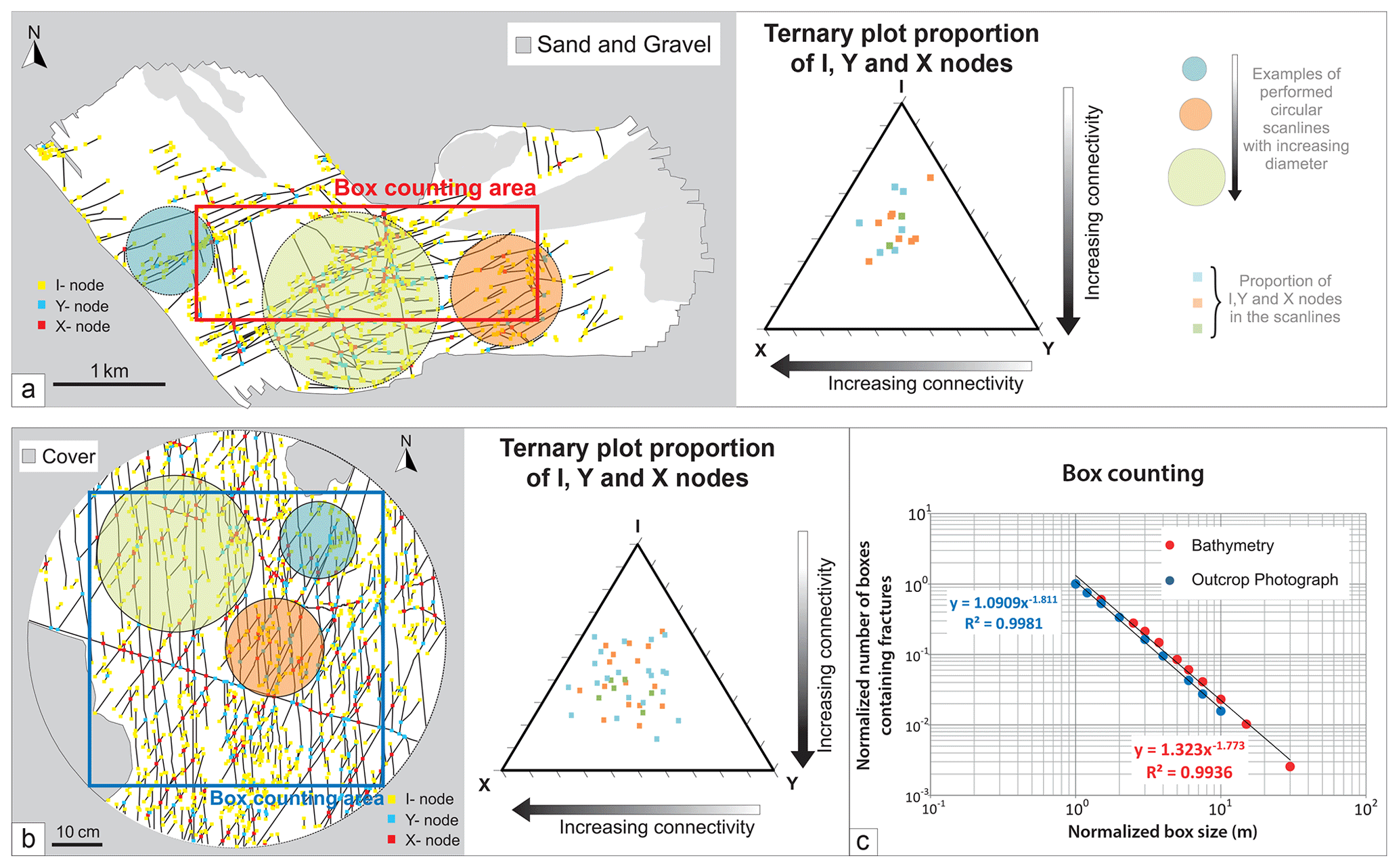
Figure 12 (a, left) 2D topological map of bathymetric data and (b, left) 2D topological map of outcrop pavement photograph (Brims Ness) showing box counting area and example of performed circular scanlines. Ternary plots of circular scanlines performed on (a, right) bathymetric data and (b, right) outcrop-scale photograph. Note that on the ternary plot from the bathymetry data the 22 circular scanlines resulted in 16 distinct proportions of I, Y and X nodes. Box counting method applied to (c) bathymetric data and (d) outcrop-scale photograph. (e) Logarithmic–logarithmic scale plot showing the result obtained from the maps in (d) and (e). Data are normalized by box size and number of fractures.

Box counting methods (Bonnet et al., 2001) were performed in the red-boxed areas shown in Fig. 12 at the mesoscale and regional scale to assess whether there is self-similarity in the 2D fracture patterns (Fig. 12a and b). Box counting assesses the presence of fractures in 2D squares of increasing size, and the box dimension should be more than 1.0 but less than 2.0 (Hirata, 1989). The normalized population plot in Fig. 12c shows a self-similarity over 1 order of magnitude for both the bathymetry (Fig. 12c, red) and the mesoscale datasets (Fig. 12c, blue). The box dimension obtained at the two different scales of analysis was −1.77 for the outcrop photograph and −1.81 for the bathymetry map (Fig. 12c). Both best-fit curves yielded R² values of 0.99. The almost identical slopes of ca −1.8 show that the 2D spatial distribution of fractures sampled at the two different ranges of scale, almost 3 orders of magnitude apart, is the same within the resolution of the box counting method.

8 Discussion

8.1 Self-similar fault and fracture scaling

Fracture attribute analyses are often conducted on field outcrop analogues because they can provide useful information to bridge the gap between faults imaged in geophysical datasets (e.g. seismic reflection profiles) and fractures observed in borehole data. Our findings show that for the aperture distributions for individual datasets – particularly at the mesoscale – the whole sample is often best described by a log-normal distribution. While it is difficult to unequivocally fit a power law due to sampling bias (truncation and censoring as discussed in Sect. 3.1.1), our new MLE approach, which progressively truncates and censors samples until the best fit emerges, shows that a power-law distribution can provide an at least equally valid, and oftentimes better, description of the data.

When our data are combined from microscale to regional scales, a power-law distribution of fracture aperture and trace length attributes emerges over 4 and 8 orders of magnitude, respectively (Fig. 8c). Variability in the fracture intensity level (y-axis intercept) and in the slope is particularly apparent for the aperture and length datasets at the mesoscale (Fig. 8c). This could be attributed to more natural variability at this scale resulting from local factors such as the proximity to major structures, lithology control or sampling. It might also be because this is the scale we have sampled the most (highest number of transect datasets). When viewed on the multiscale plot, the effect of this variability at a given scale is reduced as the plots all sit close to a power-law slope of just less than −1.0 (Fig. 8c) for both aperture and length. We suggest this approach of assessing the scaling of attributes over a large-scale range to help reduce uncertainty due to variability in individual datasets. If we are correct, then it implies that, at different magnifications (or scales), the dataset structure can be interpolated to other scales within that range. Our findings are in general agreement with Hooker et al. (2014), who found for a large number of sandstone-hosted opening-mode fractures that the aperture scaling exponent (slope) was 0.8 ± 0.1.

Mechanical stratigraphy at different scales is known to affect the aspect ratio of faults, limiting their vertical size and increasing layer-parallel growth; stratabound opening-mode fracture aperture are more likely to be log-normal (e.g. Gillespie et al., 1999). Known mechanical stratigraphic boundaries for Devonian rocks in Caithness relative to individual datasets are included in Fig. 8a (e.g. centimetre-scale beds at mesoscale), but they do not seem to affect the distribution plots, suggesting that it is not unreasonable to use power-law distributions to describe these data. The absence of a stratabound signature is consistent with the host rock being well cemented during the deformation (which is also consistent with Clair – see Sect. 2.2). Previous studies (Odling et al., 1999) of fracture length over many orders of magnitude (1 cm to 1 km) from the comparable Devonian sandstones in the Hornelen Basin (Norway) showed that, while individual datasets show log-normal distributions, the collective datasets are reasonably well described by a power-law distribution. Their 2D (when normalizing the data by area) exponent overall for joint lengths was −2.0, which would be equivalent to a value of −1.0 if normalized by length and is therefore in agreement with our study.

A number of previous studies have used data collected at one scale to extrapolate to another (for example Odling, 1999; Odling et al., 1999; Marrett et al., 1999; Hooker et al., 2009). Clearly, caution should be applied when using datasets acquired at a given scale to estimate a fracture attribute on other scales. Censored data might bias the choice of distribution function that best fits the data, suggesting that log-normal may seem more appropriate even when this is not the case in reality. However, by extending the scale observation (i.e. by applying a multiscale approach), we reduce the potential effects of censoring, truncation and variability due to individual datasets on the overall result and also extend the estimation range for the size parameters such as length, aperture and intensity. The multiscale approach, together with the analysis of truncated individual samples, has enabled us to be more confident in concluding that both single- and multiscale populations follow a power-law distribution.

Although our result remains to be tested with more datasets, the correlation we observe between aperture and length (Fig. 9) can provide a basis for a good estimation of frequency and fracture attributes for large-scale (regional) fractures (see next section). The scaling exponent (0.65) between aperture and length falls between the sub-linear (exponent = 0.5) and linear scaling (exponent = 1.0) expected for opening-mode and shear fractures (faults), respectively (Olson, 2003; Schultz et al., 2008). It is however consistent with suggestions that variations from theoretical values for the fracture length–aperture relationship are caused by interactions between segments (see Olson, 2003; Mayrhofer et al., 2019).

8.2 Applications to offshore fractured reservoirs

8.2.1 1D prediction for reservoir volumetrics

In this section we use our analogue scaling data to predict intensity, kinematic aperture and length in the Clair sub-surface reservoir, making use of a fracture model published by Coney et al. (1993). This enables us to illustrate how the analogue fracture scaling relationships established onshore can be applied to estimate sizes and intensities of fractures in sub-surface reservoirs (Fig. 13). The early fracture model was based on well and aeromagnetic data collected for Clair by Coney et al. (1993). They identified three hierarchical orders of fractures arranged in corridors (defined as closely spaced sub-parallel fractures sets) in the Clair Group spaced at 30–35 m, 100–200 m and 1–1.5 km. We regard these corridors as being equivalent to the fracture clusters we observe in our data. We assume the Clair fracture aperture and length attributes scale in a comparable way to the Caithness analogue. Aperture data collected by Franklin (2013) and observed in Clair drill core 206-13z (see example in data file in the Supplement) broadly supports this assumption. Our 1D analysis indicated fracture clusters at 3 m spacing and 600 m, and our 2D maps show corridors (clusters) spaced at sub-100 m, between 100 and 200 m, and at 1000 m. This shows that fracturing in the analogue system is behaving in a similar manner to Clair with hierarchical clustering at metre, decametre and kilometre scales. We plot the Coney et al. (1993) fracture corridor spacing on the analogue Caithness 1D scaling curves shown schematically in Fig. 13, taking into account the sub-linear length–aperture relationship established above. The reservoir spacing values (inverse of fracture intensity) provides a predictive constraint on the fracture size attributes (light grey regions) that might be expected. Predicted fracture lengths of 30–60 m length (for fractures with 30–35 m spacing), 100–150 m length (for fractures of 100–200 m spacing) and 1–2 km length (for fractures with 1–1.5 km spacing) are directly constrained by the Caithness data (dark grey area on the plot). Values of kinematic aperture can similarly be estimated. Fractures with 30–35 m spacing measured in our field analogue have estimated apertures of about 8 cm. For more widely spaced Clair structures (more than 100 m), values of aperture can be extrapolated by extending the Caithness aperture slope to larger scales (light grey area in Fig. 13). For example, for fractures spaced 100–200 m and 1–1.5 km, average aperture and fault width are estimated to be 0.8–1 and 10–20 m, respectively (light yellow lines in Fig. 13). The uncertainty in these estimates is large (see width of shaded area on the plot), and more data are needed to provide estimate errors; nonetheless the result provides an insight into the possible fracture intensity and apertures in the sub-surface reservoir.

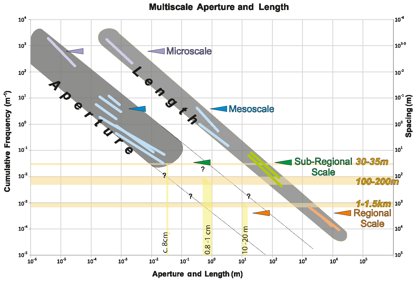
Figure 13 Sketch of the side-by-side population distribution plots of fracture lengths and apertures from Fig. 8c. The dark grey areas represent the region where all the aperture (left) and length (right) plots are localized. Coloured lines represent the distributions at each scale. Horizontal orange lines represent the reported spacing values for Clair (Coney et al., 1993), and vertical yellow lines represent the relative estimated aperture values using trends from this study. Note that we extrapolate the aperture (light grey area) using the slope derived from the microscale and mesoscale datasets.

8.2.2 2D prediction of permeability distribution

The analysis of 2D datasets using the nodal counting method has shown low connectivity for the overall systems due to the dominance of I-type nodes compared to Y- and X-type nodes. It has been suggested that areas of poor – or no – exposure greatly increase the level of subjective bias during the collection of fracture data (Andrews et al., 2019). These exposure issues tend to introduce more I nodes and decrease the estimate of connectivity. Regions of relatively higher connectivity are localized at the intersection between larger and smaller structures. The high connectivity is specific to certain areas of the 2D fracture network where fracture corridors intersect at sub-regional scale or fractures cluster at mesoscale. If fluid transport is correlated with fracture trace connectivity, we should expect the permeability and fluid transport properties within the 2D network also to be heterogeneous.

In the analogue bathymetric map dataset, we observed 1D spacing ranges similar to those observed by Coney et al. (1993) for the Clair field. We recognize 100–200 m spacing for NNW–SSE-trending faults and less than 100 m and 1 km for ENE–WSW-trending faults. Connectivity results from the bathymetry data have shown that these fractures are locally well-connected in plan view, and scanline analysis results have shown that these fractures are potentially permeable with kinematic apertures of about 10⁻¹ m, to 10 m producing, in the latter case, corridors of partially open fractures where these are clustered. These localized regions are believed to provide most of the connectivity of the 2D system and fluid flow, which is consistent with the distribution of mineralization observed in the field along corridor-type structures (e.g. the White Geos Fault locality described by Dichiarante et al., 2016).

The combination of the connectivity information in plan view derived from the bathymetry map and the fracture dip information (see Fig. 5k and l) derived from fieldwork shows that fracture corridor structures and fracture intersections will be useful in constraining the main fluid-flow anisotropy that should be considered when developing an effective drilling strategy. In general, the calculated steeply plunging fault/fracture intersections would seem to favour horizontal drilling as opposed to vertical drill orientations (Fig. 14).

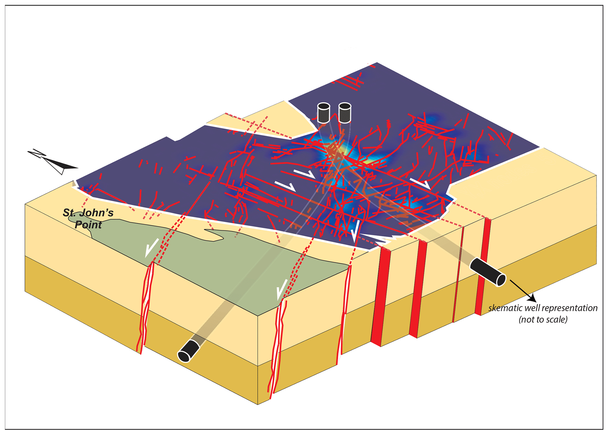
Figure 14 Schematic block diagram created by combining offshore 2D density map of connectivity and onshore dip values.

8.2.3 Application of multiscale analysis to equivalent sub-surface reservoir

Our study shows that a multiscale 1D and 2D data analysis of the Orcadian Basin analogue provides a useful insight to aid understanding of the fracture patterns in a sub-surface reservoir (in this case the Clair field). The size and scaling of aperture and length are an important control on reservoir permeability (e.g. Odling et al., 1999; Olson, 2003; Mäkel, 2007). Our mesoscale description of the aperture scaling and multiscale description of fracture length, together with the aperture–length relationship, provide a useful constraint on the 1D fracture size distributions and enable us to estimate the kinematic aperture of the largest fractures in the analogue system even though we have not sampled them directly. In doing this, we have made assumptions about the nature of the large-scale fracture corridors in the Orcadian Basin which also apply to the Clair field. The uncertainty arises in the degree to which the largest-scale structures, most likely to be faults, have a kinematic aperture in the sense of the mesoscale structures. This assumption would need to be rigorously tested using available core and image log data. The extent to which these larger fractures are likely to only be open or partially open in the sub-surface (e.g. Laubach, 2003) needs careful consideration in any application of the analogue to the sub-surface fluid flow predictions. If the decametre- to kilometre-length fractures are faults rather than opening-mode fractures, then their contribution to fluid flow may not be significant. We note that an open fracture with 14 cm kinematic aperture was recognized in drill core from well 208-8 in the Clair field (Franklin, 2013). A brecciated and mineralized fault with a width of 20 cm was recorded by Dichiarante (2017) in core 206-13z from Clair (see data file in the Supplement). Fracture fills of the kind seen in Caithness (and Clair) are not always bad for the hydrocarbon potential of a fractured reservoir. Wall rock fragments, early fracture-hosted hydrothermal minerals and fills of younger porous sediment all have the ability to act as natural proppants that hold fractures open in the long term and counteract the tendency for the present-day stress field to close open-fracture networks in sub-surface reservoirs (Holdsworth et al., 2019, 2020). These fracture fills will however reduce permeability dramatically from the “cubic law” relationships of ideal parallel-sided open fractures (Nelson, 1985; Laubach, 2003). It seems likely that both the opening-mode fractures and faults are capable of transporting fluids, therefore justifying the application of the analogue scaling relationships.

When diagenetic or other fracture fill is present, the spatial and connectivity properties have a more important impact on rock permeability (Philip et al., 2005). Our 1D fracture size analysis is extended by the 2D approach that captures fracture interaction, clustering and connectivity to describe map-scale spatial variability of the system. These relationships can be directly applied to the Clair field and other equivalent sub-surface reservoirs by calibrating the fracture size populations from drill core and image log data, the spatial properties from seismic attribute data, and the fracture fills from core description.

Finally, the methodology we employed in this study may be applied in a range of geological contexts including hydrocarbon exploration, geothermal reservoir analyses, carbon capture and deep-radioactive-waste-disposal facilities (e.g. see Primaleon et al., 2020). The straightforward multiscale approach allows direct comparison between analogues and sub-surface targets and is easy to apply to different areas, dataset types and scales to provide important constraints for reservoir modelling and prediction at regional scales.

9 Conclusions

The Devonian rocks of the Orcadian Basin in Caithness provide a plausible analogue for the main reservoir in the Clair field and other equivalent offshore fractured reservoirs hosted in similar tight sandstone strata. We applied a multiscale fracture analysis methodology as an alternative to the use of single-scale datasets to characterize the fracture attributes. We advocate an extended approach that integrates datasets collected at different scales and combines 1D and 2D analysis. In our example, statistical analysis provides a useful insight into the nature and scalability of the natural fracture networks. Our work has a number of specific findings:

•  

  Our 1D analysis has shown that the population distribution of length and aperture of the onshore datasets are best described using truncated power-law distributions.

•  

  The multiscale approach shows scale invariance. The scalability of a single dataset can be extended from 1–2 orders of magnitude (single plots) to up to 4 and 8 orders of magnitude (side-by-side plots) for aperture and trace length, respectively. This illustrates that the multiscale approach improves the confidence using power-law scaling distributions to describe natural fracture systems.

•  

  The correlation between fracture aperture and length is well represented by sub-linear power-law scaling (exponent = 0.65) over 4 orders of magnitude. Although this remains to be tested with more microscale datasets and understanding of the large-scale fault properties, we suggest that this methodology provides a good estimation of fracture attributes and their scaling properties.

•  

  Using the normalized spatial correlation approach, we detected fracture clusters at 3 and 600 m. In 2D, we observed fracture corridors spaced at < 100, 150 and 100 m.

An associated topological 2D analysis has provided the following additional insights:

•  

  Box counting methods have shown the self-similarity of fracture counts over about 1 order of magnitude at bathymetry and outcrop scales. The datasets have almost identical slopes, showing that the fracture arrays over different scale ranges have the same 2D spatial distribution, which confirms the hierarchical scaling of fracture clusters from the spatial analysis.

•  

  The overall connectivity of the 2D system is low and very similar on the two scales of observation studied. However, connectivity is highly variable in the system and appears to be mainly focused along fracture corridors or clusters at a large scale and on the longer structures at the mesoscopic outcrop scale.

Our study demonstrates how a multiscale 1D size distribution and 2D spatial analysis of an onshore analogue may provide a better understanding of fracture scaling in a geologically equivalent sub-surface reservoir, in this example the Clair reservoir. The method allows a prediction of fracture or fault size and their clustering properties. The spatial information, in particular, together with fracture geometry (i.e. dip data) provides important constraints on the possible permeability anisotropy. The nature of fracture fills and in situ stress should also be considered when planning exploratory drilling or modelling the reservoir.