the Creative Commons Attribution 4.0 License.
the Creative Commons Attribution 4.0 License.
 | 30 Apr 2020
An active tectonic field for CO2 storage management: the Hontomín onshore case study (Spain)
José F. Mediato
Miguel A. Rodríguez-Pascua
Jorge L. Giner-Robles
Adrià Ramos
Silvia Martín-Velázquez
Roberto Martínez-Orío
Paula Fernández-Canteli
One of the concerns of underground CO2 onshore storage is the triggering of induced seismicity and fault reactivation by the pore pressure increasing. Hence, a comprehensive analysis of the tectonic parameters involved in the storage rock formation is mandatory for safety management operations. Unquestionably, active faults and seal faults depicting the storage bulk are relevant parameters to be considered. However, there is a lack of analysis of the active tectonic strain field affecting these faults during the CO2 storage monitoring. The advantage of reconstructing the tectonic field is the possibility to determine the strain trajectories and describing the fault patterns affecting the reservoir rock. In this work, we adapt a methodology of systematic geostructural analysis to underground CO2 storage, based on the calculation of the strain field from kinematics indicators on the fault planes (ey and ex for the maximum and minimum horizontal shortening, respectively). This methodology is based on a statistical analysis of individual strain tensor solutions obtained from fresh outcrops from the Triassic to the Miocene. Consequently, we have collected 447 fault data in 32 field stations located within a 20 km radius. The understanding of the fault sets' role for underground fluid circulation can also be established, helping further analysis of CO2 leakage and seepage. We have applied this methodology to Hontomín onshore CO2 storage facilities (central Spain). The geology of the area and the number of high-quality outcrops made this site a good candidate for studying the strain field from kinematics fault analysis. The results indicate a strike-slip tectonic regime with maximum horizontal shortening with a 160 and 50∘ E trend for the local regime, which activates NE–SW strike-slip faults. A regional extensional tectonic field was also recognized with a N–S trend, which activates N–S extensional faults, and NNE–SSW and NNW–SSE strike-slip faults, measured in the Cretaceous limestone on top of the Hontomín facilities. Monitoring these faults within the reservoir is suggested in addition to the possibility of obtaining a focal mechanism solutions for micro-earthquakes (M<3).
- Article
(19761 KB) - Full-text XML
- BibTeX
- EndNote


Industrial human activities generate CO2 that could change the chemical balance of the atmosphere and their relationship with the geosphere. Geological carbon storage (GSC) appears as a good choice to reduce the CO2 gas emission to the atmosphere (Christensen and Holloway, 2004), allowing industry to increase activity with a low pollution impact. There is a lot of literature about what a site must have to be a potential underground storage suitable to GSC (e.g., Chu, 2009; Orr, 2009; Goldberg et al., 2010 among others). Reservoir sealing, caprock, permeability and porosity, plus injection pressure and volume injected, are the main considerations to choose one geological subsurface formation as the CO2 host rock. In this context, the tectonically active field is considered in two principal ways: (1) to prevent the fault activation and earthquakes triggering, with the consequence of leakage and seepage, and (2) the long-term reservoir behavior, understanding long-term as a centennial to millennial time span. Therefore, what is the long-term behavior of GSC? What do we need to monitor for safe GSC management? Winthaegen et al. (2005) suggest three subjects for monitoring: (a) the atmosphere air quality near the injection facilities, due to the CO2 toxicity (values greater than 4 %; see Rice, 2003, and Permentier et al., 2017), (b) the overburden monitoring faults and wells, and (c) the sealing of the reservoir. The study of natural analogs for GSC is a good strategy to estimate the long-term behavior of the reservoir, considering parameters such as the injected CO2 pressure and volume, plus the brine mixing with CO2 (Pearce, 2006). Hence, the prediction of site performance over long timescales also requires an understanding of CO2 behavior within the reservoir, the mechanisms of migration out of the reservoir, and the potential impacts of a leak on the near-surface environment. The assessments of such risks will rely on a combination of predictive models of CO2 behavior, including the fluid migration and the long-term CO2–porewater–mineralogical interactions (Pearce, 2006). Once again, the tectonically active field interacts directly with this assessment. Moreover, the fault reactivation due to the pore pressure increasing during the injection and storage also has to be considered (Röhmann et al., 2013). Despite the uplift measured by Röhmann et al. (2013) being sub-millimeter (ca. 0.021 mm) at the end of the injection processes, given the ongoing occurrence of micro-earthquakes, long-term monitoring is required. The geomechanical and geological models predict the reservoir behavior and the caprock sealing properties. The role of the faults inside these models is crucial for the tectonic long-term behavior and the reactivation of faults that could trigger earthquakes.
Concerning induced seismicity, Wilson et al. (2017) published the Hi-Quake database, with a classification of all man-made earthquakes according to the literature, in an online repository (https://inducedearthquakes.org/, last access: May 2019). This database includes 834 projects with proved induced seismicity, where two different cases with earthquakes as large as M=1.7, detected in swarms of about 9500 micro-earthquakes, are related to GSC operations. Additionally, Foulger et al. (2018) pointed out that GSC can trigger earthquakes with magnitudes less than M=2: the cases described in their work are as great as M=1.8, with the epicenter location 2 km around the facilities. McNamara (2016) described a comprehensive method and protocol for monitoring a GSC reservoir for the assessment and management of induced seismicity. The knowledge of active fault patterns and the stress or strain field could help design a monitoring network and identify those faults capable of triggering micro-earthquakes (M<2) and/or breaking the sealing for leakage (patterns of open faults for low-permeability CO2 migration).
In this work, we propose that the description, the analysis and establishment of the tectonic strain field have to be mandatory for long-term GSC monitoring and management, implementing the fault behavior in the geomechanical models. This analysis does not increase the cost of long-term monitoring, given that it is low-cost and the results are acquired in a few months. Therefore, we propose a methodology based on the reconstruction of the strain field from the classical studies in geodynamics (Angelier, 1979, 1984; Reches, 1983, 1987). As an innovation, we introduce the strain field (SF) analysis between 20 km away from the subsurface reservoir deep geometry, under the area of influence of induced seismicity for fluid injection. The knowledge of the strain field at a local scale allows classifying the type of faulting and their role for leakage processes, whilst the regional scale explores the tectonically active faults that could affect the reservoir. The methodology is rather simple, taking measures of slickensides and striations on fault planes to establish the orientation of the maximum horizontal shortening (ey) and the minimum horizontal shortening (ex) for the strain tensor. The principal advantage of the SF analysis is the direct classification of all the faults involved in the geomechanical model and the prediction of the failure parameters. Moreover, a Mohr–Coulomb failure analysis was performed on the fault pattern recognized in the Cretaceous outcrop located on top of the pilot plant.
The tectonic characterization of the GSC of Hontomín was implemented in the geological model described by Le Gallo and de Dios (2018). Beyond the use of induced seismicity and potentially active faults, the scope of this method is to propose an initial analysis to manage underground storage operations. We present how the structural analysis of fault or slip data can improve the knowledge on the tectonic large-scale fault network for the potential seismic reactivation during fluid injection and the time-dependent scale of fluid stays.
2.1 Geological description of the reservoir
The CO2 storage site of Hontomín is enclosed in the southern section of the Mesozoic Basque–Cantabrian Basin, known as the Burgalesa Platform (Serrano and Martínez del Olmo, 1990; Tavani, 2012), within the sedimentary Bureba Basin (Fig. 1). This geological domain is located in the northern junction of the Cenozoic Duero and Ebro basins, forming an ESE-dipping monocline bounded by the Cantabrian Mountain Thrust to the north, the Ubierna Fault System (UFS) to the south and the Asturian Massif to the west (Fig. 1).
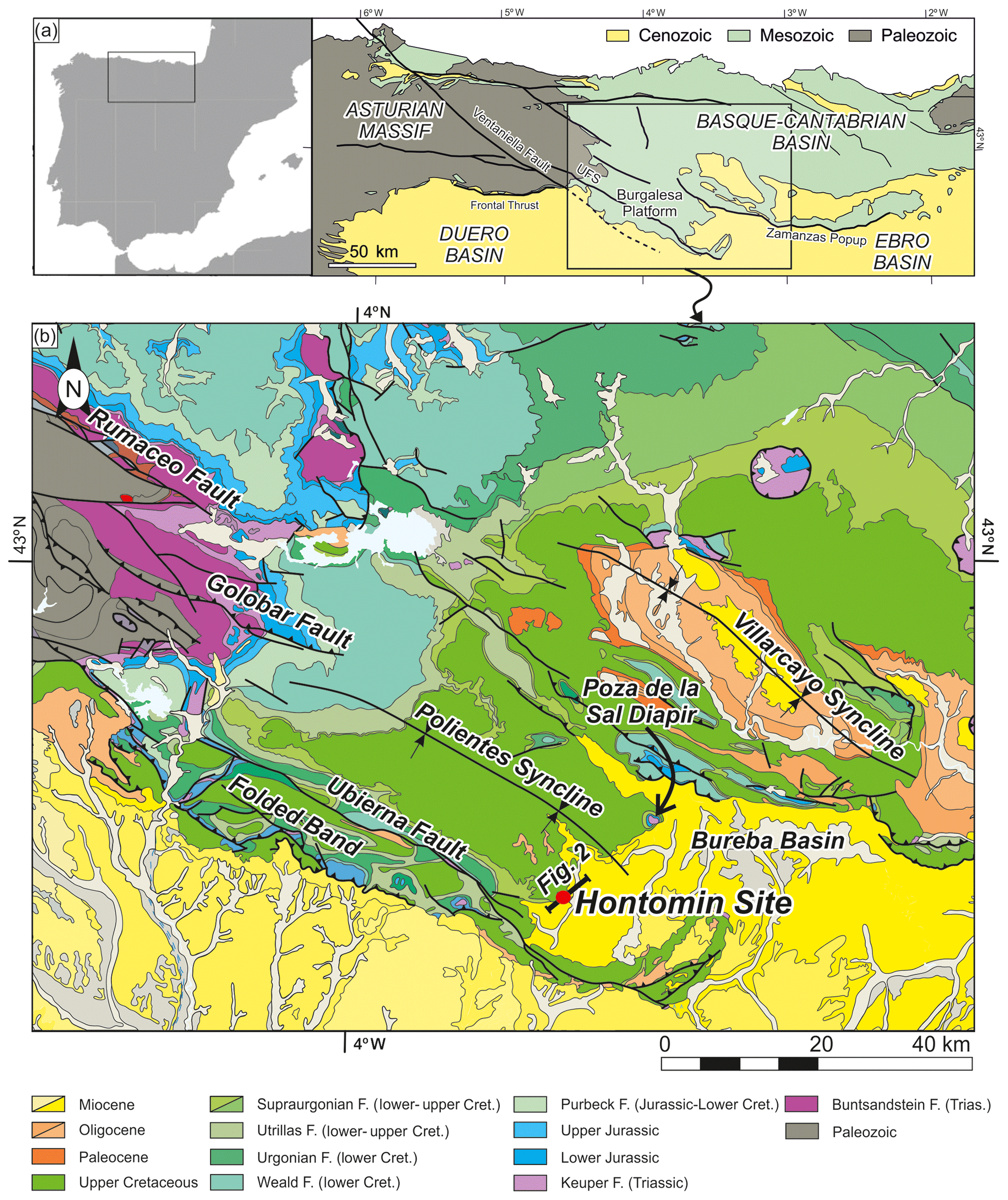
Figure 1(a) Location map of the study area in the Iberian Peninsula, along with the geological map of the Asturian and Basque–Cantabrian areas, labeling major units and faults (modified after Quintà and Tavani, 2012); (b) geographical location of Hontomín pilot plant (red dot) within the Basque–Cantabrian Basin. This basin is tectonically controlled by the Ubierna Fault System (UFS; NW–SE-oriented) and the parallel Polientes syncline, the Duero and Ebro Tertiary basins, and Poza de la Sal evaporitic diapir. Cret: Cretaceous; F: facies.
The Meso-Cenozoic tectonic evolution of the Burgalesa Platform starts with a first rift period during Permian and Triassic times (Dallmeyer and Martínez-García, 1990; Calvet et al., 2004), followed by relative tectonic quiescence during Early and Middle Jurassic times (e.g., Aurell et al., 2002). The main rifting phase took place during Late Jurassic and Early Cretaceous times, due to the opening of the North Atlantic and the Bay of Biscay-Pyrenean rift system (García-Mondéjar et al., 1986; Le Pichon and Sibuet, 1971; Lepvrier and Martínez-García, 1990; García-Mondéjar et al., 1996; Roca et al., 2011; Tugend et al., 2014). The convergence between Iberia and Eurasia from Late Cretaceous to Miocene times triggered the inversion of previous Mesozoic extensional faults and the development of an E–W orogenic belt (Cantabrian domain to the west and Pyrenean domain to the east) formed along the northern Iberian plate margin (Muñoz, 1992; Gómez et al., 2002; Vergés et al., 2002).
The Hontomín facilities are located within the Basque–Cantabrian Basin (Fig. 1b). The geological reservoir structure is bordered by the UFS to the south and west, by the Poza de la Sal diapir and the Zamanzas Popup structure (Carola, 2014) to the north, and by the Ebro Basin to the east (Fig. 1). The structure is defined as a forced fold-related dome structure (Tavani et al., 2013; Fig. 2), formed by an extensional fault system with migration of evaporites towards the hanging wall during the Mesozoic (Soto et al., 2011). During the tectonic compressional phase, associated with the Alpine Orogeny affecting the Pyrenees, the right-lateral transpressive inversion of the basement faults was activated, along with the reactivation of transverse extensional faults (Fig. 2; Tavani et al., 2013; Alcalde et al., 2014).

Figure 2Interpretation of a 2-D seismic reflection profile crossing the oil exploration wells (H1, H2 and H4), along with the monitoring well (Ha) and injection well (Hi) through Hontomín pilot plant (HPP). Modified from Alcalde et al. (2014). See Fig. 1 for location; black line at the red circle.
The target reservoir and seal formations consist of Lower Jurassic marine carbonates, arranged in an asymmetric dome-like structure (Fig. 2) with an overall extent of 15 km2 and located at 1485 m depth (Alcalde et al., 2013, 2014; Ogaya et al., 2013). The target CO2 injection point is a saline aquifer formed by a dolostone unit, known as “Carniolas”, and an oolitic limestone of the Sopeña Formation, both corresponding to Lias in time (Early Jurassic). The estimated porosity of the Carniolas reaches over 12 % (Ogaya et al., 2013; Le Gallo and de Dios, 2018), and it is slightly lower at the Carbonate Lias level (8.5 % in average). The reservoir levels contain saline water with more than 20 g L−1 of NaCl and very low oil content. The high porosity of the lower part of the reservoir (i.e., the Carniolas level) is the result of secondary dolomitization and different fracturing events (Alcalde et al., 2014). The minimum thickness of the reservoir units is 100 m. The potential upper seal unit comprises Lias marlstones and black shales from a hemipelagic ramp (Fig. 2; Pliensbachian and Toarcian) of the “Puerto del Pozazal” and Sopeña formations.
2.2 Regional tectonic field
The tectonic context has been described from two different approaches: (1) the tectonic style of the fractures bordering the Hontomín reservoir (De Vicente et al., 2011; Tavani et al., 2011) and (2) the tectonic regional field described from earthquakes with mechanism solutions and GPS data (Herraiz et al., 2000; Stich et al., 2006; De Vicente et al., 2008).
-
The tectonic style of the Bureba Basin was described by De Vicente et al. (2011), which classified the Basque–Cantabrian Cenozoic Basin (Fig. 1a) as transpressional with a contractional horsetail splay basin. The NW–SE-oriented Ventaniella Fault (Fig. 1a) includes the UFS in the southeastward area, being active between the Permian and Triassic period and strike-slip during the Cenozoic contraction. In this tectonic configuration, the Ubierna Fault acts as a right-lateral strike-slip fault. These authors pointed out the sharp contacts between the thrusts and the strike-slip faults in this basin. Furthermore, Tavani et al. (2011) also described a complex Cenozoic tectonic context where a right-lateral tectonic style reactivated WNW-ESE-trending faults. Both the Ventaniella and the Ubierna faults acted as transpressive structures, 120 km long and 15 km wide and featuring 0.44 mm yr−1 averaged tectonic strike-slip deformation between the Oligocene and the present day. The aforementioned authors described different surface segments of the UFS of right-lateral strike-slip ranging between 12 and 14 km length. The structural data collected by Tavani et al. (2011) pointed out that 60 % of data correspond to right-lateral strike-slip with a WNW–ESE trend, together with conjugate reverse faulting with a NE–SW, NW–SE and E–W trend, and left-lateral strike-slip faults N–S-oriented. They concluded that this scheme could be related to a transpressional right-lateral tectonic system with a maximum horizontal compression, SHmax, striking 120∘ E. Concerning the geological evidence of recent sediments affected by tectonic movements of the UFS, Tavani et al. (2011) suggest the middle Miocene in time for this tectonic activity. However, geomorphic markets (river and valley geomorphology) could indicate tectonic activity at present times. All of these data correspond to regional or small-scale data collected to explain the Basque–Cantabrian Cenozoic transpressive basin. The advantage of the methodology proposed here to establish the tectonic local regime affecting the reservoir is the search for local-scale tectonics (with a size of 20 km) and the estimation of the depth for the non-deformation surface for strata folding in transpressional tectonics (Lisle et al., 2009).
-
Regarding the stress field from earthquake focal mechanism solutions, Herraiz et al. (2000) pointed out the regional trajectories of SHmax with a NNE–SSW trend, and with a NE–SW SHmax trend from slip-fault inversion data. Stich et al. (2006) obtained the stress field from seismic moment tensor inversion and GPS data. These authors pointed out a NW–SE Africa–Eurasia tectonic convergence at a tectonic rate of approximately 5 mm yr−1. However, no focal mechanism solutions are found within the Hontomín area (20 km) and only long-range spatial correlation could be made with high uncertainty (in time, space and magnitude). The same lack of information appears in the work of De Vicente et al. (2008), with no focal mechanism solutions in the 50 km surrounding the Hontomín pilot plant (HPP). In this work, these authors classified the tectonic regime as a uniaxial extension to strike-slip with a NW–SE SHmax trend.
Regional data about the tectonic field inferred from different works (Herraiz et al., 2000; Stich et al., 2006; De Vicente et al., 2008, 2011; Tavani et al., 2011; Tavani, 2012) show differences for the SHmax. These works explain the tectonic framework for the regional scale. Nevertheless, local tectonics could determine the low permeability and the potential induced seismicity within the reservoir. In the next section, we have applied the methodology described at Sect. 3 of this paper, in order to compare the regional results from these works.
2.3 Strategy of the ENOS European project
HPP for CO2 onshore storage is the only one in Europe recognized as a key test facility, and it is managed and conducted by CIUDEN (Fundación Ciudad de la Energía). The HPP is located within the province of Burgos (Fig. 1b), in the northern central part of Spain.
The methodology proposed in this work and its application for long-term onshore GSC management in the context of geological risk is based on the strain tensor calculation, as part of the objectives proposed in the European project ENabling Onshore CO2 Storage in Europe (ENOS). The ENOS project is an initiative of CO2GeoNet, the European Network of Excellence on the geological storage of CO2, to support onshore storage and highlight the associated problems, such as GSC perception, safe storage operation, potential leakage management, and health and environmental safety (Gastine et al., 2017). ENOS combines a multidisciplinary European project, which focuses in onshore storage, with the demonstration of best practices through pilot-scale projects in the case of the Hontomín facilities. Moreover, this project claims to create a favorable environment for GSC onshore through public engagement, knowledge sharing and training (Gastine et al., 2017). In this context, the work-package WP1 is devoted to “ensuring safe storage operations”.
The lithosphere remains in a permanent state of deformation, related to plate tectonic motion. Strain and stress fields are the consequence of this deformation on the upper lithosphere, causing different fault patterns that determine sedimentary basins and geological formations. The kinematics of these faults describe the stress or strain fields, for example measuring grooves and slickensides on fault planes (see Angelier, 1979, and Reches, 1983, among others). The relevance of the tectonic field is that stress and strain determine the earthquake occurrence by the fault activity. In this work, we have performed a brittle analysis of the fault kinematics by measuring slickenfiber on fault planes (dip–dip direction and rake), in several outcrops in the surroundings of the onshore reservoir. To carry out the methodology proposed in this work, the study area was divided into a circle with four equal areas, and we searched outcrops of fresh rock to perform the fault kinematic analysis. This allows establishing a realistic tectonic very near field to be considered during the storage seismic monitoring and long-term management. Finally, we have studied the fault plane reactivation by using the Mohr–Coulomb failure criterion (Pan et al., 2016) from the fault pattern obtained in the Cretaceous limestone outcrop located on top of the HPP facilities.
3.1 Paleostrain analysis
We have applied the strain inversion technique to reconstruct the tectonic field (paleostrain evolution), affecting the Hontomín site between the Triassic, Jurassic, Cretaceous and Neogene ages (late Miocene to present times). For a further methodological explanation, see Etchecopar et al. (1981), Reches (1983) and Angelier (1990). The main assumption for the inversion technique of fault population is the self-similarity to the scale invariance for the stress or strain tensors. This means that we can calculate the whole stress or strain fields by using the slip data on fault planes and for homogeneous tectonic frameworks. The strain tensor is an ellipsoid defined by the orientation of the three principal axes and the shape of the ellipsoid (k). This method assumes that the slip vectors, obtained from the pitch of the striation on different fault planes, define a common strain tensor or a set in a homogeneous tectonic arrangement. We assume that the strain field is homogeneous in space and time, the number of faults activated is greater than five and the slip vector is parallel to the maximum shear stress (τ).
The inversion technique is based on the Bott equations (Bott, 1959). These equations show the relationship between the orientation and the shape of the stress ellipsoid:
where l, m and n are the direction cosines of the normal to the fault plane, θ is the pitch of the striation and R′ is the shape of the stress ellipsoid obtained in an orthonormal coordinate system, x, y, z. In this system, σy is the maximum horizontal stress, σx is the minimum horizontal stress axis and σz is the vertical stress axis.
3.2 The right-dihedral model for paleostrain analysis
The right-dihedral (RD) is a semiquantitative method based on the overlapping of compressional and extensional zones by using a stereographic plot. The final plot is an interferogram figure, which usually defines the strain regime. This method is strongly robust for conjugate fault sets and with different dip values for the same tensor. The RD was originally defined by Pegoraro (1972) and Angelier and Mechler (1977), as a geometric method, adjusting the measured fault-slip data (slickensides) in agreement with theoretical models for extension and compressive fault slip. Therefore, we can constrain the regions of maximum compression and extension related to the strain regime.
3.3 The slip model for the paleostrain analysis
The slip model (SM) is based on the Navier–Coulomb fracturing criteria (Reches, 1983), taking the Anderson model solution for this study (Anderson, 1951; Simpson, 1997). The Anderson model represents the geometry of the fault plane as monoclinic, relating the quantitative parameters of the shape parameter (K′) with the internal frictional angle for rock mechanics (φ) (De Vicente, 1988; Capote et al., 1991). Moreover, this model is valid for neoformed faults, and some considerations have to be accounted for for previous faults and weakness planes present in the rock. These considerations are related to the dip of normal and compressional faults, such as for compressional faulting dip values lower than 45∘, reactivated as extensional faults. This model shows the relationships between the K′, φ and the direction cosines for the striation on the fault plane (De Vicente, 1988; Capote et al., 1991):
where ez is the vertical strain axis, ey is the maximum horizontal shortening and ex is the minimum horizontal shortening. This model assumes that there is no change in volume during the deformation and .
For isotropic solids, principal strain axes coincide with the principal stress axes. This means that in this work, the orientation of the principal stress axis, SHmax, is parallel to the orientation of the principal strain axes, ey, and, hence, the minimum stress axis, Shmin, is parallel to the minimum strain axis, ex. This assumption allows us to estimate the stress trajectories (SHmax and Shmin) from the ey SM results.
Resolving the equations of Anderson for different values (Anderson, 1951), we can classify the tectonic regime that activates one fault from the measurement of the fault dip, sense of dip (0–360∘) and pitch of the slickenside, assuming that one of the principal axes (ex, ey or ez) is vertical (Angelier, 1984). We can classify the tectonic regime and represent the strain tensor by using the ey and ex orientation.
3.4 The K′-strain diagram
Another analysis can be achieved by using the K′-strain diagram developed by Kaverina et al. (1996) and codified in Python code by Álvarez-Gómez (2014). These authors have developed a triangular representation based on the fault slip, where tectonic patterns can be differentiated as strike-slip and dip-slip types. This diagram is divided into seven different zones according to the type of fault: (1) pure normal, (2) pure reverse and (3) pure strike-slip; these were combined with the possibility of oblique faults ((4) reverse strike-slip and (5) strike-slip with a reverse component) and lateral faults ((6) normal strike-slip and (7) strike-slip faults with a normal component; Fig. 3). Strike-slip faults are defined by small values for pitch (p<25∘) and dips close to vertical planes (β>75∘). High pitch values (p>60∘) are related to normal or reverse fault-slip vectors. Extensional faults show ey in the vertical, whereas compressional faults show ey in the horizontal plane.
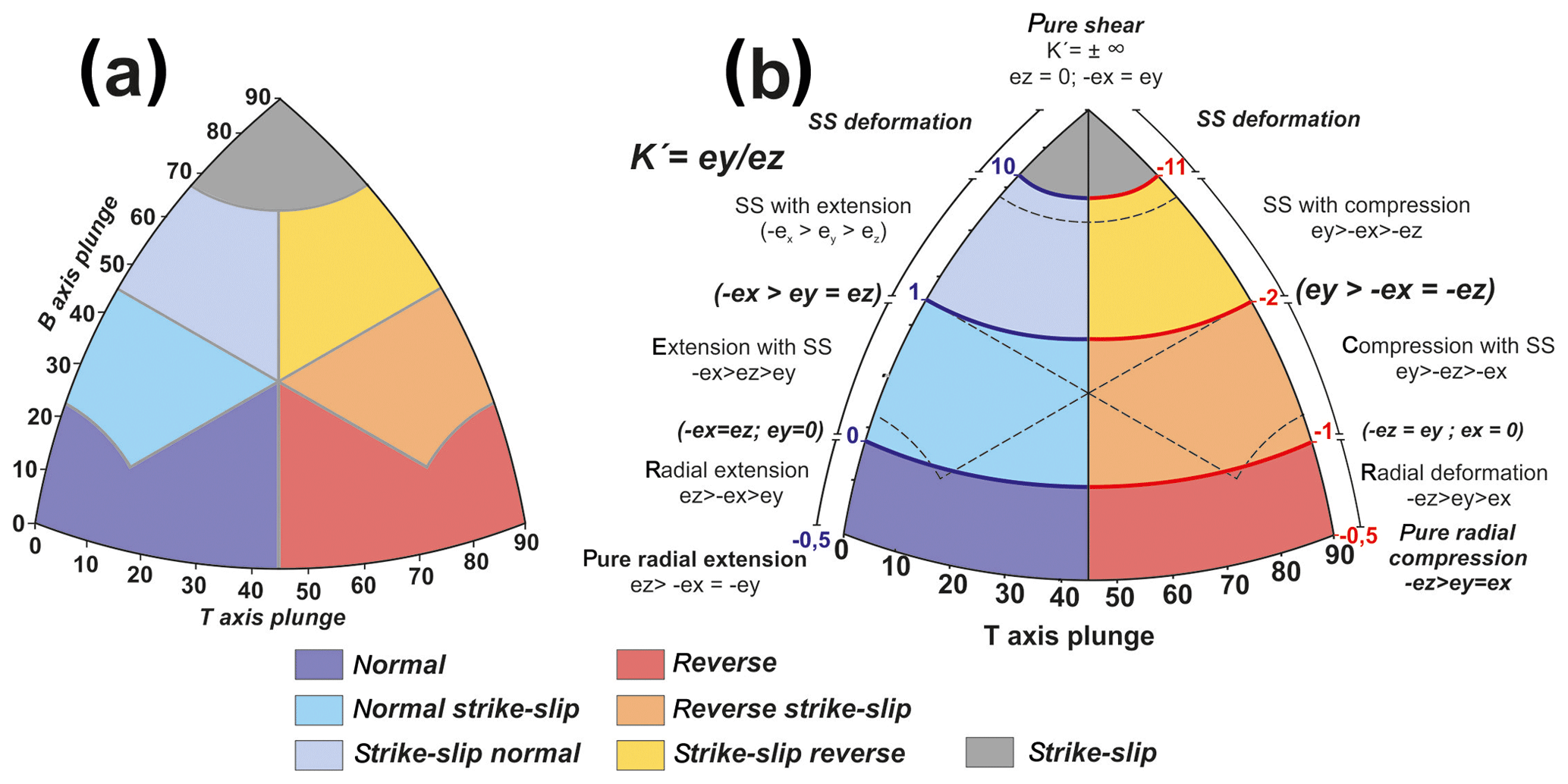
Figure 3(a) Kaverina original diagram to represent the tectonic regime from an earthquake focal mechanism population (see Kaverina et al., 1996, and Álvarez-Gómez, 2014). (b) K′-strain diagram used in this work. Dotted lines represent the original Kaverina limits. Colored zones represent the type of fault. The tectonic regime is also indicated by the relationship between the strain axes and the colored legend. SS: strike-slip. The B axis is orthogonal to the P and T axes.
This method was originally performed for earthquake focal mechanism solutions by using the focal parameters, the nodal planes (dip and strike) and rake (Kaverina et al., 1996). The triangular graph is based on the equal-area representation of the T, N, or B and P axes in spherical coordinates (T tensile, N or B neutral, and P pressure axes) and the orthogonal regression between earthquake magnitudes Ms and mb for the Harvard earthquake Global CMT (Centroid Moment Tensor) catalogue in 1996. Álvarez-Gómez (2014) presented a Python-based for computing the Kaverina diagrams, and we have modified the input parameters by including the K′ intervals for the strain field from the SM. The relationship between the original diagram of Kaverina (Fig. 3a) and the K′-strain diagram (Fig. 3b) that we have used in this work is shown in Fig. 3. The advantage of this diagram is the fast assignation of the type of fault and the tectonic regime that determines this fault pattern and the strain axes relationship.
Table 1 summarizes the different tectonic regimes of Fig. 3b showing the relationship with the strain main axes ey, ex and ez. This diagram exhibits a great advantage to classify the type of fault according to the strain tensor. Therefore, we can assume the type of fault from the fault orientation affecting geological deposits for each strain tensor obtained.
Table 1Different tectonic regimes, K′ values, dip values and fault type for the Kaverina modified diagram used in this work. According to the strain axes relationship, faults can be classified and the tectonic regime can be established.
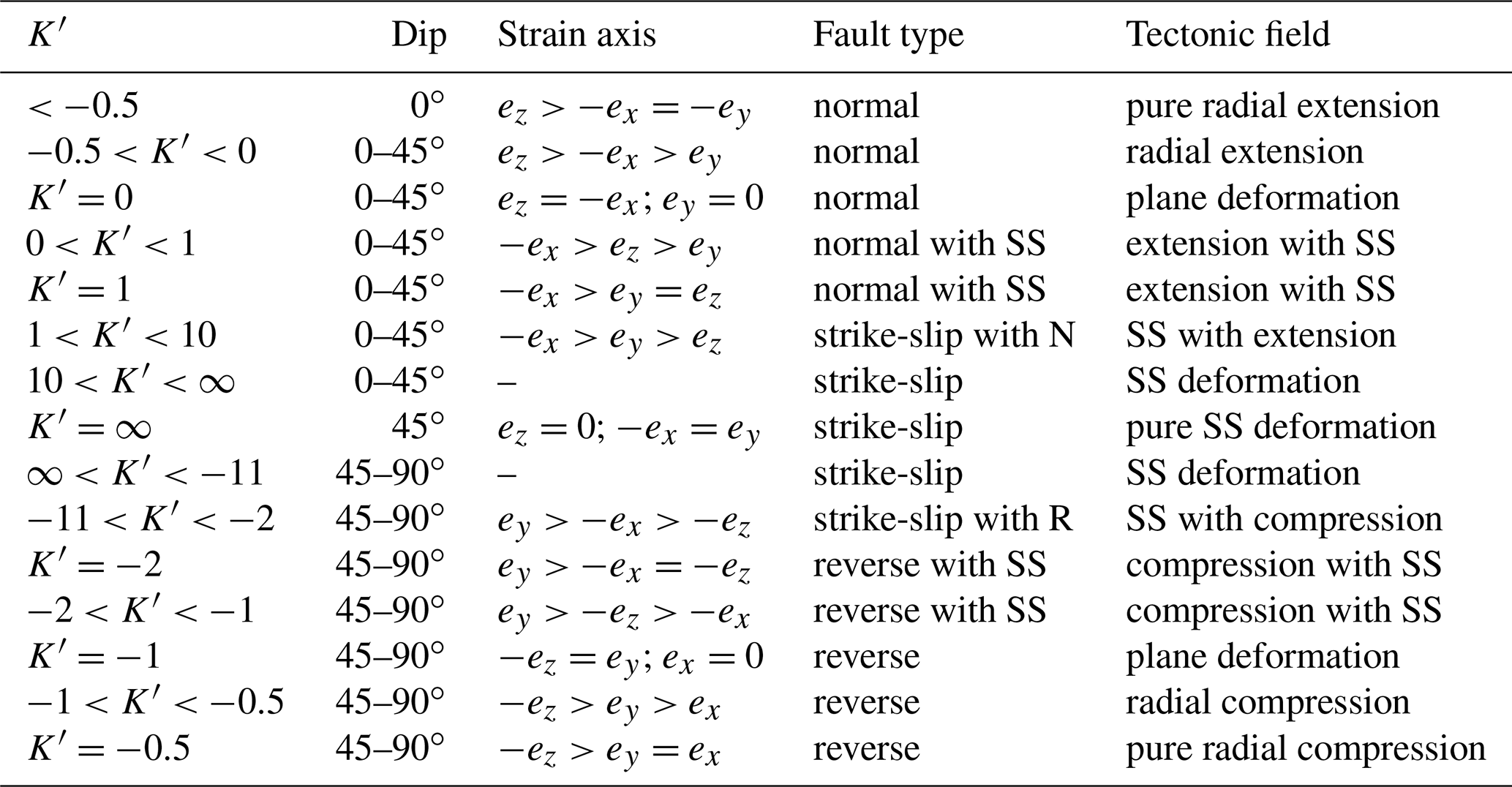
SS: strike-slip; ex=Shmin: minimum horizontal shortening; N: normal; ey=SHmax: maximum horizontal shortening; R: reverse and ez: vertical axis.
3.5 The circular-quadrant-search (CQS) strategy for the paleostrain analysis
In this work, we propose a low-cost strategy based on a well-known methodology for determining the stress or strain tensor affecting a GSC reservoir, which will allow the long-term monitoring of geological and seismic behavior (Fig. 4). The objective is to obtain enough structural data and spatially homogeneous of faults (Figs. 4 and 5) for reconstructing the stress or strain tensor. The key point is the determination of the orientation of the ey, ex and K′ to plot on a map and, therefore, to establish the tectonic regime. We have chosen quadrants of the circles with the aim to obtain a high-quality spatial distribution of point for the interpretation of the local and very near strain field. Hence, data are homogeneously distributed, instead of being only concentrated in one quadrant of the circle.
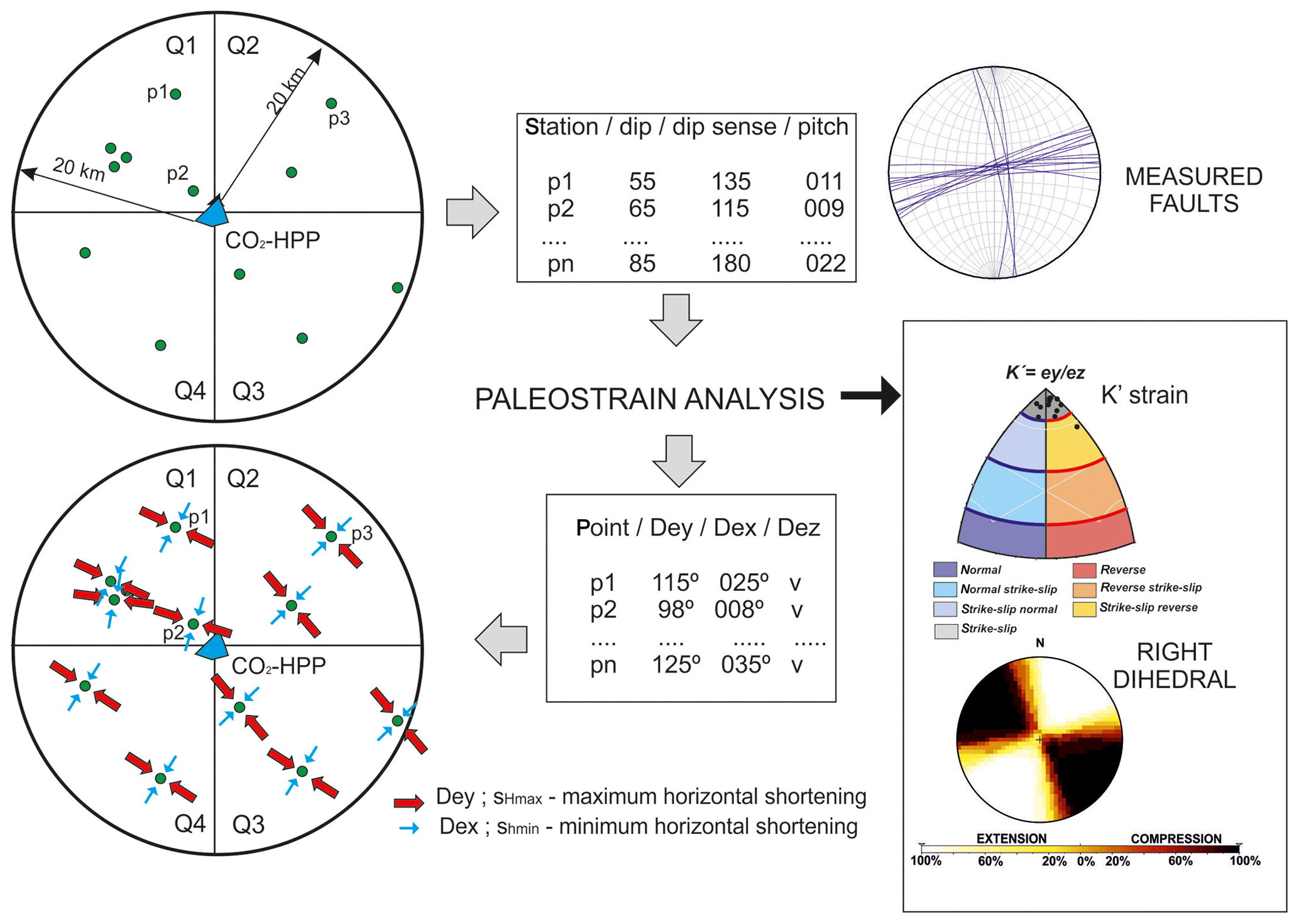
Figure 4Methodology proposed to obtain the strain field affecting the GSC reservoir. The distances for outcrops and quadrants proposed is 20 km. The technique of right-dihedral and the K′-strain diagram is described in the main text. The ey and ex represented are a model for explaining the methodology. Dey and Dex are the direction of the maximum and minimum strain, respectively. Blue box at the center is the CO2 storage geological underground formation.
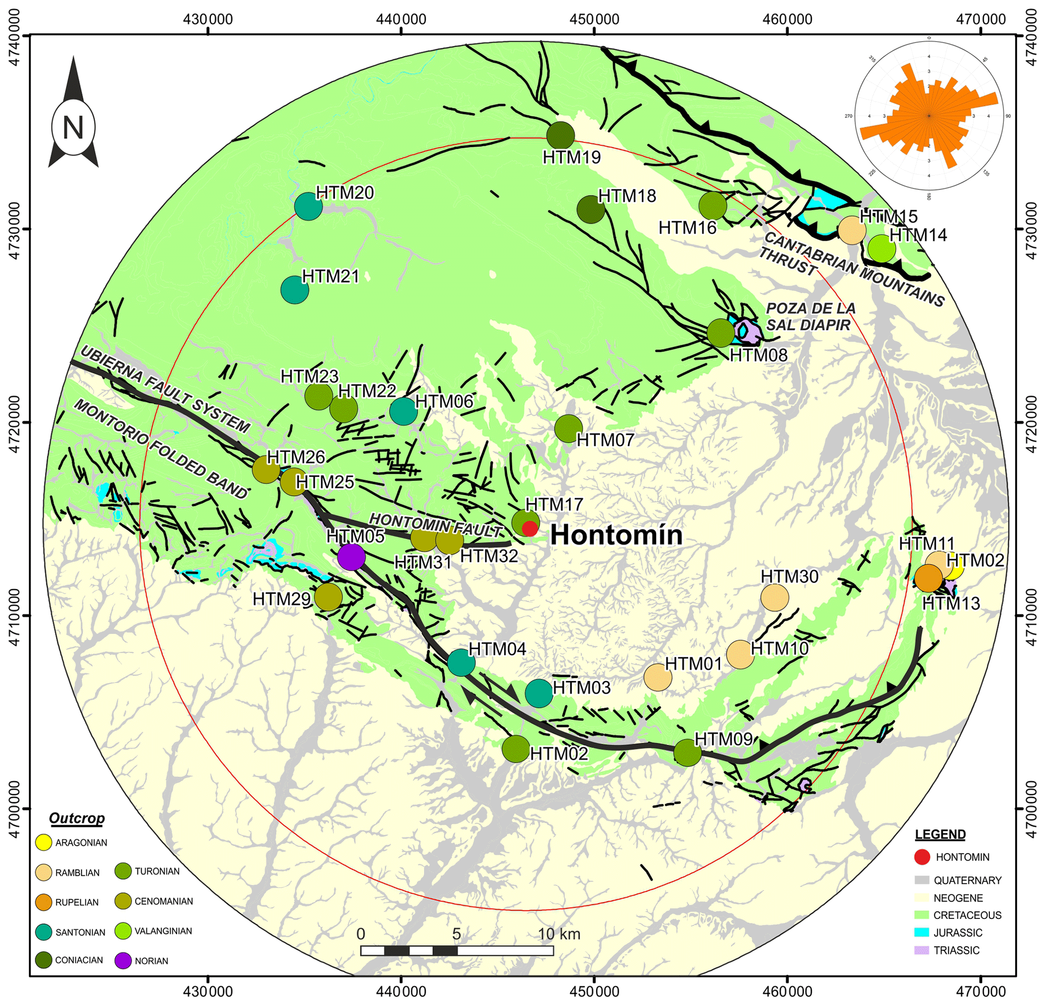
Figure 5Geographical location of field outcrops in the eastern part of the Burgalesa Platform domain. Black lines: observed faults; red circle: 20 km radius study zone. Rose diagram are the fault orientations from the map. A total of 447 fault data were collected in 32 outcrops. Data were measured by a tectonic compass on fault planes at outcrops. The spatial distribution of the field stations is constrained by the lithology. Coordinates are in meters, UTM H30.
Pérez-López et al. (2018) carried out a first approach to the application of this methodology at Hontomín, under the objective of the ENOS project (see next section for further details). We propose a circular searching of structural field stations (Figs. 4 and 5), located within a 20 km radius. This circle was chosen, given that active faults with the capacity of triggering earthquakes of magnitudes close to M=6 exhibit a surface rupture of tens of kilometers, according to empirical models (Wells and Coppersmith, 1994). Moreover, Verdon et al. (2015) pointed out that the maximum distance of induced earthquakes for fluid injection is 20 km. Larger distances could not be related to the stress or strain regime within the reservoir, except for the case of large geological structures (folds, master faults, etc.). Microseismicity in GSC reservoir is mainly related to the operations during the injection or depletion stages and long-term storage (Verdon, 2014; Verdon et al., 2015; McNamara, 2016).
The presence of master faults (capable of triggering earthquakes of magnitude = or > than a 6 and 5 km long segment) inside the 20 km radius circle implies that the regional tectonic field determines the strain accumulation in a kilometric fault size. Furthermore, the presence of master faults could increase the occurrence of micro-earthquakes, due to the presence of secondary faults prone to triggering earthquakes by their normal seismic cycle (Scholz, 2018). It must be borne in mind that GSC onshore reservoirs used to be deep saline aquifers (e.g., Bentham and Kirby, 2005) as in the case of Hontomín (Gastine et al., 2017; Le Gallo and de Dios, 2018), which is confined in folded and fractured deep geological structures, in which local tectonics plays a key role in micro-seismicity and the possibility of CO2 leakage.
The constraints of this strategy are related to the absence of kinematic indicators on fault planes. This absence could occur due to later overlapping geological processes as neoformed mineralization. Also, a low rigidity eludes the slickenfiber formation, and no kinematic data will be marked on the fault plane. A poor spatial distribution of the outcrops was also taken into account for constraining the strategy. The age of sediments does not represent the age of the active deformations, and, hence, the active deformation has to be analyzed by performing alternative methods (i.e., paleoseismology, archaeoseismology).
4.1 Strain field analysis
We have collected 447 fault-slip data points on fault planes in 32 outcrops, located within a 20 km radius circle centered at the HPP (Fig. 5). The age of the outcrops ranges from Early Triassic to post-Miocene, and they are mainly located in Cretaceous limestone and dolostone (Fig. 5, Table 2). However, no Jurassic outcrops were located, and only seven stations are located on Neogene sediments, ranging between early Oligocene to middle–late Miocene. The small number of Neogene stations is due to the mechanical properties of the affected sediments, mainly poorly lithified marls and soft-detrital fluvial deposits. Despite that, all the Neogene stations exhibit high-quality data with a number of fault-slip data ranging between 7 and 8, enough for a minimum quality analysis.
Table 2Summary of the outcrops showing the number of faults, the type of the strain tensor obtained, the Dey, SHmax striking and the age of the affected geological materials. N-C is the normal component for strike-slip movement.
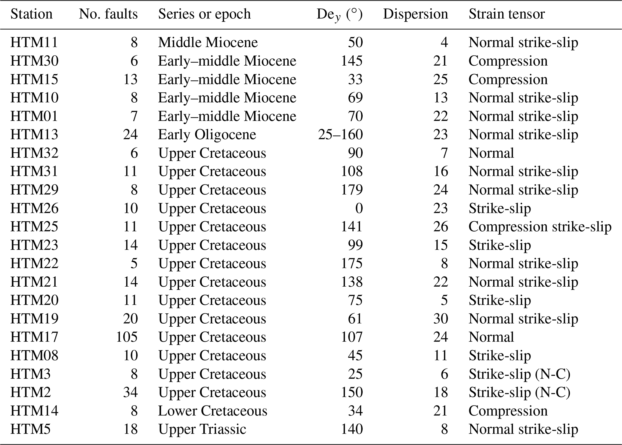
We have labeled the outcrops with the acronym HTM followed by a number (see Fig. 5 for the geographical location and Table 2 and Fig. 6 for the fault data). The station with the highest number of faults measured is HTM17 with 105 faults on Cretaceous limestone. Conjugate fault systems can be recognized in most of the stations (HTM1, 3, 5, 7, 10, 14, 16, 21, 23, 24, 25, 29, 30 and 32; Fig. 6), although there are a few stations with only one well-defined fault set (6, 22, 32). We have to bear in mind that the recording of conjugate fault systems is more robust for the brittle analysis than recording isolated fault sets, better constraining the solution (Žalohar and Vrabec, 2008). In total, 29 of 32 stations were used (HTM24, 27, 28 with no quality data), and of these 29 stations, 21 were analyzed with the paleostrain technique. Solutions obtained here are robust to establish the paleostrain field in each outcrop as the orientation of ey, SHmax (Fig. 7).
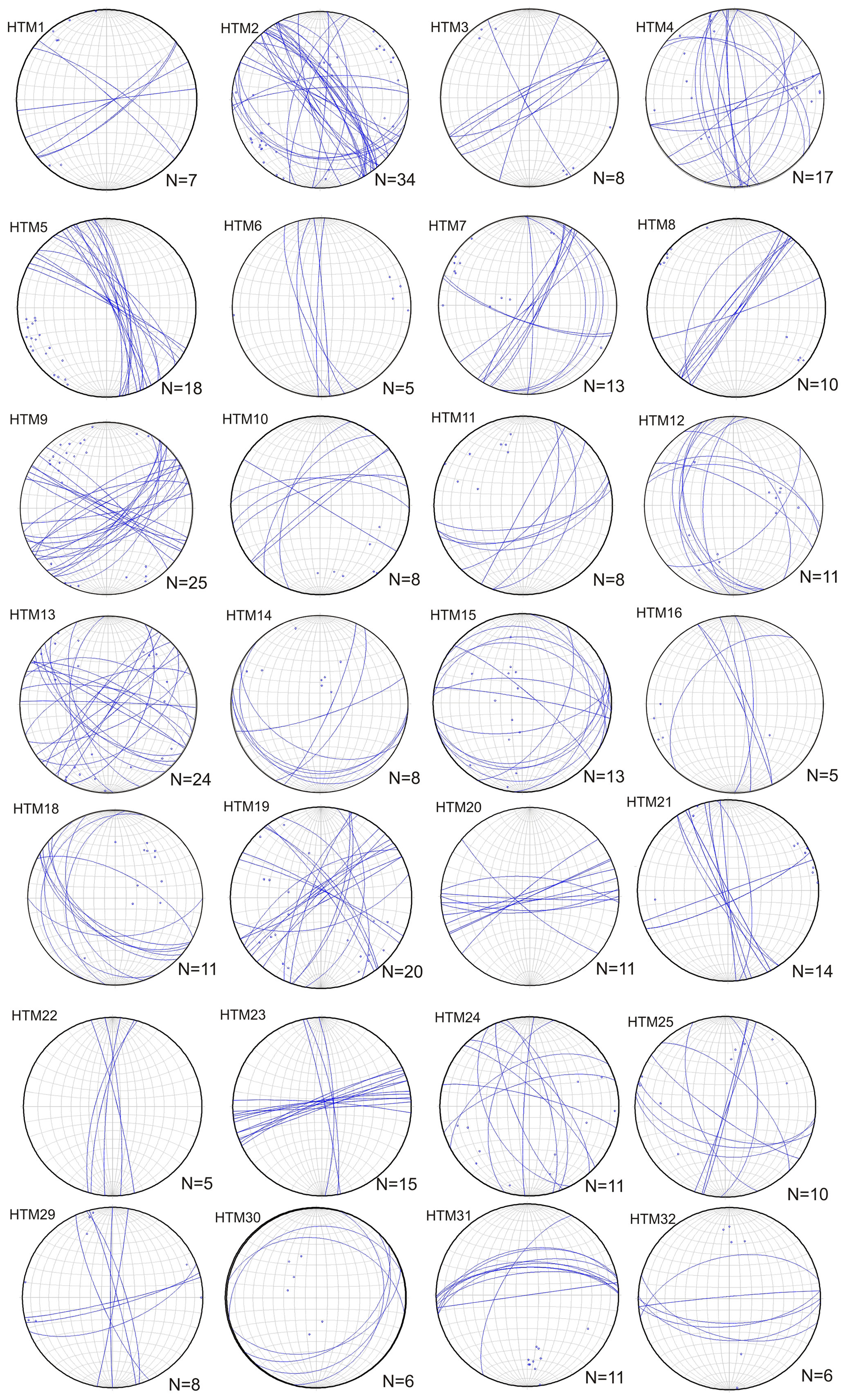
Figure 6Stereographic representation (cyclographic plot in Schmidt net, lower hemisphere) of the fault planes measured in the field stations. “n” is the number of available data for each geostructural station. HTM24, 27 and 28 are not included due to lack of data, and HTM17 is not included due to the high number of faults.
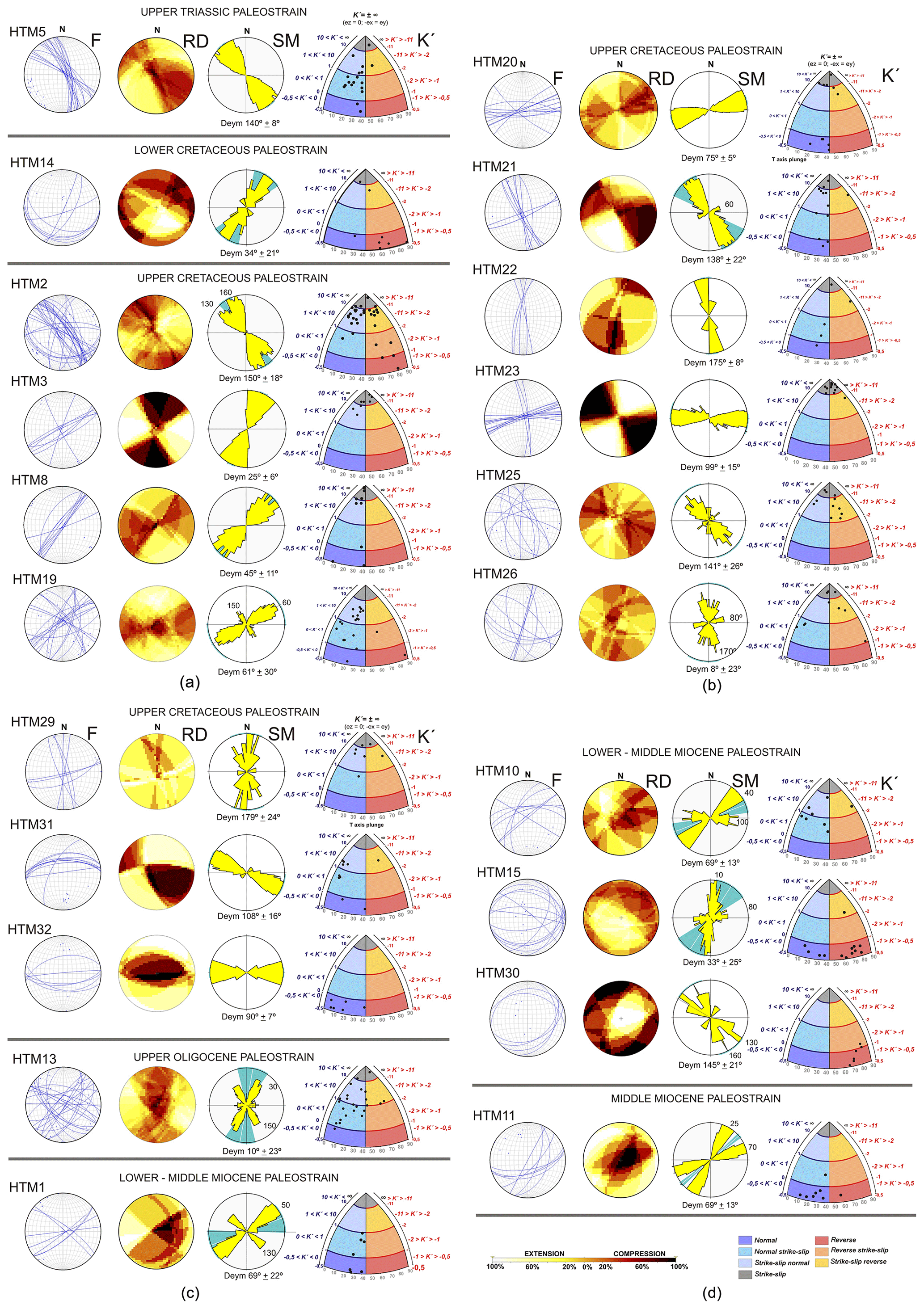
Figure 7Results of the paleostrain analysis obtained and classified by age. Deym: striking of the averaged of the Dey value; F: fault stereographic representation; K′-strain diagram with dots for each fault-slip solution; RD: right-dihedral method; SM: slip method. See the Methods section for further explanation.
The results obtained from the application of the paleostrain method have been expressed in a stereogram, RD, SM and a K′-strain diagram (Fig. 7). The K′-strain diagram shows the fault classification as normal faults, normal with strike-slip component, pure strike-slip, strike-slip with reverse component and reverse faults (see Fig. 3). The main faults are lateral strike-slips and normal faults, followed by reverse faults, strike-slips and oblique strike-slips faults. The results of the strain regime are as follows: (1) 43 % of extensional with shear component; (2) 22 % of shear; (3) 13 % of compressive strain (Lower Cretaceous and early–middle Miocene, Table 2); (4) 13 % of pure shear and (5) 9 % of shear with compression strain field, although with the presence of five reverse faults.
In contrast, we can observe that there are solutions with a double value for the ey, SHmax orientation: HTM1, 2, 10, 11, 13, 15, 19, 26, and 30. The stations HTM3 and 23 (Upper Cretaceous) show the best solution for a strike-slip strain field as a pure strike-slip regime and ey with a 25 and 99∘ E trend, respectively (Fig. 7).
It is easy to observe the agreement between the ey results from the SM and the K′-strain diagram; for instance, in the HTM2 the K′-strain diagram indicates strike-slip faults with a reverse component for low dips () but also indicates strike-slip faults with a normal component for larger dips (). However, both results are in agreement with a strain field defined by the orientation for ey, SHmax with trend. This tectonic field affects Cretaceous carbonates and coincides with the regional tectonic field proposed by Herraiz et al. (2000), Tavani et al. (2011) and Alcalde et al. (2014).
4.2 Late Triassic outcrop paleostrain
Strain analysis from the HTM5 fault set shows ey with a NW–SE-trending and shear regime with the extension defined by strike-slip faults (Fig. 7a). This is in agreement with the uniaxial extension described in Tavani (2012), constraining this regime with SHmin with a NE–SW trend.
4.3 Cretaceous outcrop paleostrain
We have divided this result in two groups: (a) outcrops within the 20 km circle from HPP and (b) the outcrop of the HTM17 (Fig. 5), which is located in the HPP facilities and described in the next section. HTM14 is the only outcrop of Early Cretaceous age, showing a compressive tectonic stage with reverse fault solutions, defined by ey with a NE–SW trend (Fig. 7a–c). Taking into account the extensional stage related to the main rifting stage that took place in Early Cretaceous times (i.e., Carola, 2014; Tavani, 2012; Tugend et al., 2014), we interpreted these results as a modern strain field, probably related to the Cenozoic inversion stage.
Outcrops HTM2, 3, 8, 17, 19, 20, 21, 22, 23, 25, 26, 29, 31 and 32 are from the Upper Cretaceous carbonates (Fig. 7). Results are as follows: (1) a compressive strain stage featured by ey with a NW–SE trend, similar to the stage described in Tavani (2012), and (2) a normal strain stage with ey striking both E–W and NE–SW (Fig. 7, HTM20, 21, 31 and 32). Finally, a (3) shear stage (activated strike-slip faults) and (4) a shear with extension (strike-slip with normal component) were described as well. These two late stages are featured by ey with NE–SW and NW–SE trends. The existence of four different strain fields is determined by different ages during the Cretaceous and different spatial locations in relation to the main structures, the Ubierna Fault System, Hontomín Fault, Cantabrian Thrust, Montorio folded band and the Polientes syncline (Fig. 1).
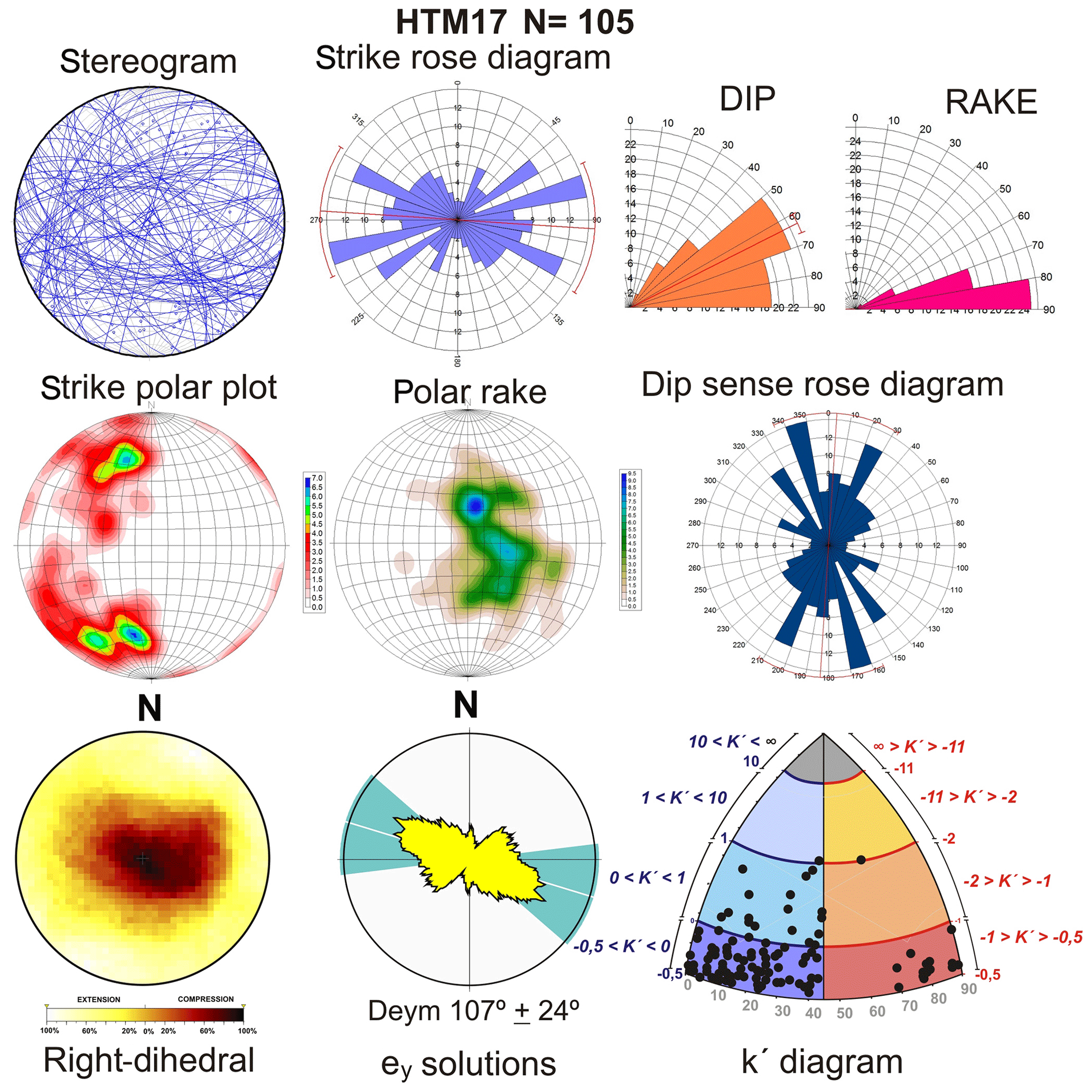
Figure 8Fault data from the outcrop HTM17 located on top of the HPP. See Fig. 5 for the geographical location. Stereogram plot is lower hemisphere and Schmidt net.
4.4 Cretaceous outcrop HTM17 on the Hontomín pilot plant
This outcrop is located on top of the geological reservoir, in a quarry of Upper Cretaceous limestones. The main advantage of this outcrop is the good development of striation and carbonate microfibers which yields high-quality data. Overall, 105 fault-slip data were measured, with the main orientation striking 75,−50 ∘E and a conjugate set with a 130∘ E (±10∘) trend (Fig. 8). The result of the strain inversion technique shows an extensional field featuring an ey trajectory striking 107∘ E (±24∘) related to an extensional strain field (see the K′-strain diagram in Fig. 8). Most of the faults are extensional faults NE–SW and NW–SE-oriented (Fig. 9), in agreement with the extensional RD solution. Reverse faults are oriented NNE–SSW, E–W and WNW–ESE. The advantage of this outcrop is the geographical and stratigraphic position. It is located on top of the HPP facilities in younger sediments than the reservoir rocks. Furthermore, given that the Jurassic reservoir rock and the Cretaceous upper unit are both composed of carbonates, the fault pattern measured here could be a reflex of the fracture network affecting the Jurassic storage rocks at depth (see Figs. 2 and 9).
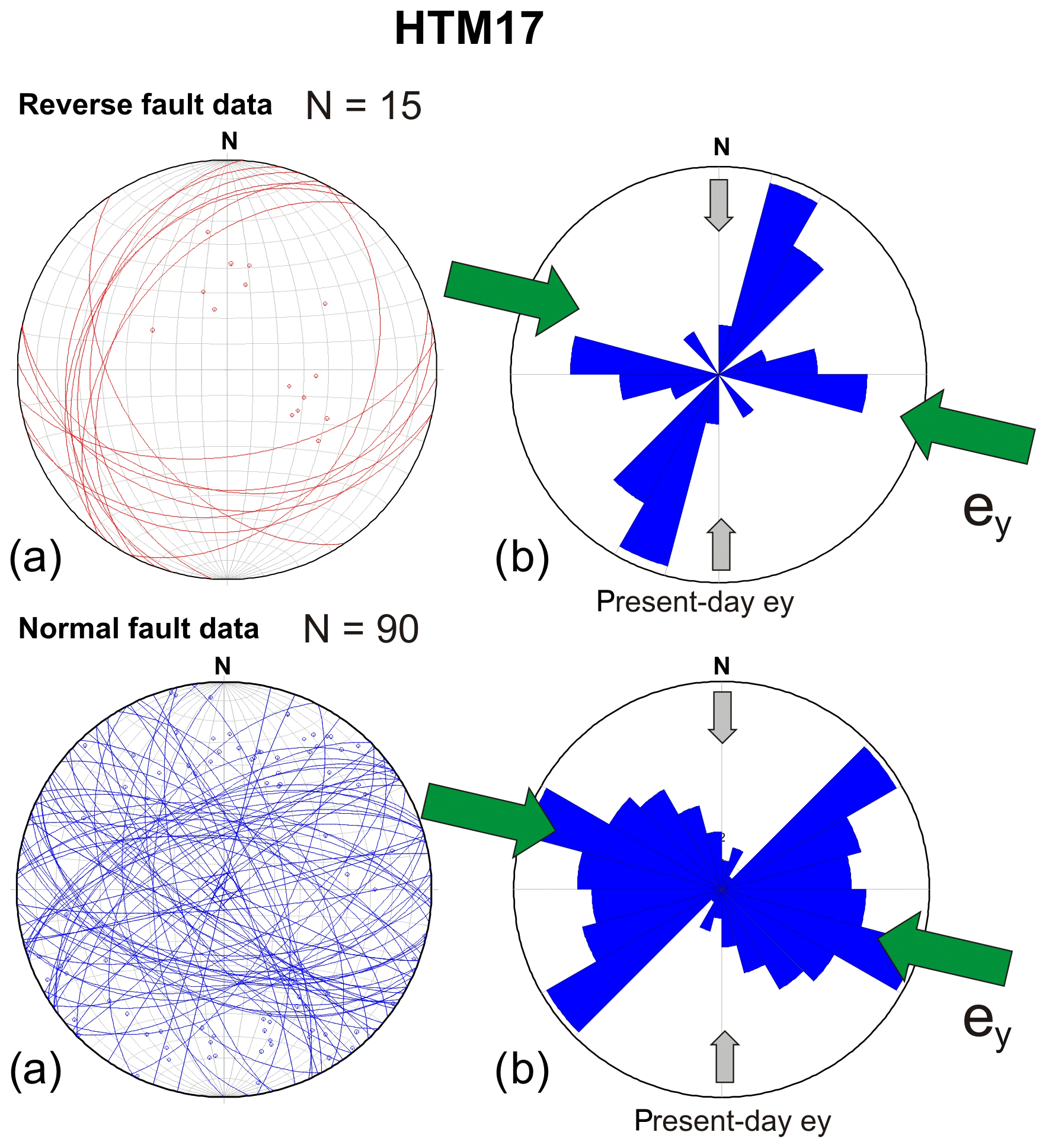
Figure 9Normal and reverse faults stereograms (lower hemisphere and Schmidt net), and rose diagrams measured in HTM17. Green arrows indicate the orientation of the local paleostrain field. Grey arrows indicate the orientation of the present-day regional stress field (Herraiz et al., 2000).
4.5 Cenozoic outcrop strain field
The Cenozoic tectonic inversion in the area has been widely described by different authors (e.g., Carola, 2014; Tavani, 2012; Tungend et al., 2014). This tectonic inversion is related to compressive structures, activating NE–SW and ENE–WSW thrusts with NW–SE and NNE–SSW ey trends, respectively. The Ubierna Fault has been inverted with right-lateral transpressive kinematics during the Cenozoic (Tavani et al., 2011). The Early Oligocene outcrop (HTM13, Fig. 7c) shows a local extensional field with ey with a NNE–SSW and 150∘ E trend. During the lower–middle Miocene, HTM15 and HTM30 outcrops exhibit the same ey trend, but for a compressive tectonic regime (Fig. 7d). HTM1 shows extensional tectonics with ey oriented 50 and 130∘ E. Summarizing, the Cenozoic inversion and tectonic compression are detected during the early to middle Miocene and the Oligocene. However, during the middle Miocene only one extensional stage was interpreted (HTM1, Fig. 7c).
The outcrops located closer to the HPP (HTM17, 31, 32, Figs. 5 and 7) show E–W faults. HTM5 is located on the Ubierna Fault, showing a NW–SE trend, whilst HTM3 shows NE–SW strike-slip.
Strain analysis suggests that the planes parallel to the SHmax orientation (NNW–SSE and N–S) could induce the leakage into the reservoir (Fig. 7). Moreover, a 50∘ E SHmax orientation could also affect the reservoir. HPP facilities are close to the Hontomín Fault (Fig. 5), a WNW–ESE-oriented fault, although the HTM17 station shows that N–S fault planes could play an important role for seepage of fluid into the reservoir.
5.1 Regional active stress tensor in HTM17 fault pattern
The active regional field proposed by Herraiz et al. (2000), Stich et al. (2006), Tavani et al. (2011) and Alcalde et al. (2014) shows ey, SHmax with almost NNW–SSE and N–S trends. Namely, the work from Herraiz et al. (2000) calculates three stress tensors within the 20 km of our study area and a Quaternary stress tensor close to the area (ca. 40 km south of Hontomín). The age of the first one is Miocene and defined by σ1 87∕331∘; σ2 01∕151∘; σ3 00∕061∘ (dip–dip sense 0–360∘), with an R=0.06 and SHmax trending 151∘ E, under an extensional tectonic regime. Two post-Miocene stress tensors are defined by (1) σ1 87∕299∘; σ2 00∕209∘; σ3 01∕119∘ with R=0.13, SHmax with a 29∘ E trend under an extensional tectonic regime and (2) σ1 00∕061∘; σ2 86∕152∘; σ3 03∕331∘, with R=0.76, and SHmax 62∘ E under a strike-slip tectonic regime. Finally, these authors calculated a Quaternary stress tensor defined by σ1 85∕183∘; σ2 02∕273∘; σ3 03∕003∘; R=0.02 and SHmax with a 101∘ E trend under an extensional tectonic regime. The regional active stress tensor defined for Pliocene–Quaternary ages is σ1 88∕197∘; σ2 01∕355∘; σ3 00∕085∘ for 327 data with R=0.5 and SHmax with an N–S trend under an extensional tectonic regional regime.
We have applied the regional active stress tensor (Herraiz et al., 2000) for studying the reactivation of previous fault patterns measured in HTM17 (Figs. 8 and 9). To carry out this study, we assume that the fault plane reactivation depends on σ1 and σ3 and the shape of the failure envelope. Therefore, we have used the Mohr–Coulomb failure criteria for preexisting fault planes (Xu et al., 2010; Labuz and Zang, 2012), by using the MohrPlotter v3.0 code (Allmendinger et al., 2012). Moreover, to calculate the Mohr–Coulomb circle, it is necessary to know the cohesion and friction parameters of the reservoir rock. Bearing in mind that the reservoir rocks are Lower Jurassic carbonates (dolostone and oolitic limestone; Alcalde et al., 2013, 2014; Ogaya et al., 2013), we have assumed the averaged cohesion for carbonates (limestone and dolostone) at 35∘ and the coefficient of internal friction of 0.7 (Goodman, 1989). In addition, we have assumed no cohesion with an angle of static friction of 0.7 for preexisting faults.
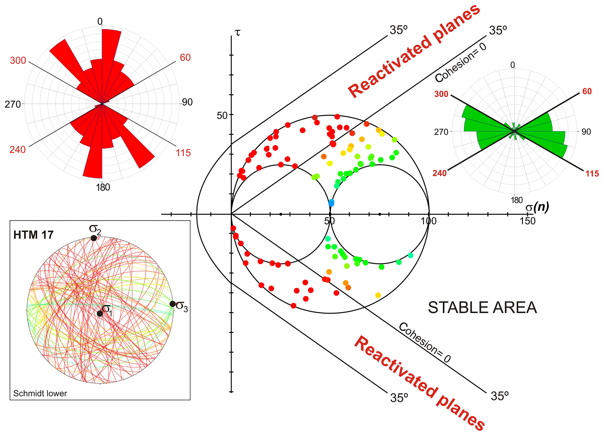
Figure 10Mohr–Coulomb failure analysis for the fault-slip data measured in HTM17 under the present-day stress tensor determined by Herraiz et al. (2000). Red dots are faults reactivated, and green and orange dots are located within the stable zone. Red rose diagram shows the orientation of reactivated faults, between N–S and 60∘ E and from 115 to 180∘ E. Green rose diagram shows the fault orientation for faults non-reactivated under the active stress field within the area. See text for further details. The yellow data in the Mohr–Coulomb (M–C) diagrams refer to those planes close to being reactivated and potentially reactivated by increasing the pore pressure.
Figure 10 shows the main results for the Mohr analysis. The reactivated planes under the active present stress field are red dots: 52 of the original 105 fault-slip measurements at HTM17. Green and orange dots indicate faults with no tectonic strength accumulation under the present-day stress field. Reactivated fault sets are oriented between N to 60∘ E and 115 to 180∘ E, with N–S and NNE–SSW as the main trends (Fig. 10, red rose diagram). Under an extensional tectonic field with R=0.5, N–S are normal faults, whereas NNE–SSW and NNW–SSE trends are strike-slips faults with extensional components. According to the results shown in Fig. 10, these faults could be reactivated without a pore pressure increase. The inactive fault orientation is constrained between 60 and 115∘ E, mainly WNW–ESE (Fig. 10, green rose diagram). Regarding the uncertainties of these fault orientations, these values can oscillate ±5∘, according to the field error measurement (averaged error for measuring structures by a compass).
Concerning the reliability of the results, some constraints need to be explained. The Mohr–Coulomb failure criterion is an approximation that assumes that the normal stress on the fault plane is not tensile. Furthermore, the increases in pore pressure in the reservoir rock reduces the normal stress on the plane of failure, and the interval of fault reactivation could be higher. This effect was not considered in the previous analysis since the calculation of the critical pore pressure is beyond the purpose of this work. Nevertheless, the MohrPlotter software (Allmendinger et al., 2012) allows estimating the increase of pore pressure to the critical value under some conditions.
Finally, we have applied the slip model and right-dihedral to the reactivated fault-slip data from the HTM17 outcrop (Fig. 11), by including the rake estimated from the active regional stress tensor determined by Herraiz et al. (2000). At a glance, faults oriented between 10∘ E and 10∘ W act as normal faults (4 out 52, Fig. 11a and c), faults between 10–50∘ E and 10–50∘ W act as extensional faults with strike-slip components (31 out 52), and NE–SW and NW–SE vertical faults act as pure strike-slips (8 out 52). The right-dihedral shows a tectonic regime of strike-slip with extensional component (see De Vicente et al., 1992), with orthorhombic symmetry and SHmax oriented 10∘ W, which is in agreement with the stress tensor proposed by Herraiz et al. (2000) with ∘ and σ1 vertical. However, strain analysis in this case shows a strike-slip extensional tectonic regime instead of the extensional regime derived from the stress field. Despite this, both the Mohr–Coulomb analysis and the paleostrain analysis (SM and RD) suggest N–S normal faulting, NNE–SSW to NE–SW and NNW–SSE to NW–SE strike-slips as the active fault network affecting the reservoir. De Vicente et al. (1992) pointed out that the SM analysis is more robust applied to fault-slip data classified previously by other techniques. Here, we have used the Mohr–Coulomb failure criteria to separate active fault sets under the same strain tensor, yielding robustness to the results from SM and RD analysis.
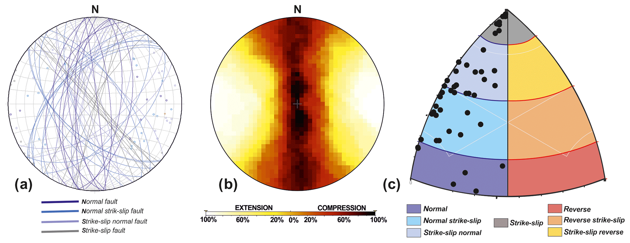
Figure 11(a) Stereogram and poles of fault sets (HTM17) reactivated under the present-day stress field suggested by Herraiz et al. (2000). (b) right-dihedral of the reactivated fault sets. (c) K′-strain diagram showing the type of fault for each fault set.
We propose as complementary and future work a combined analysis consisting of the fault population analysis and the slip-tendency analysis (Morris et al., 1996), which could improve and identify those fault sets most likely to be reactivated under an active stress field. Although both analyses (fault population and slip tendency) are based on the stress tensor and the orientation of fault traces, the slip tendency also includes rock strength values obtained from the “in situ” tests.
5.2 Active faulting in the surroundings of HPP
Quaternary tectonic markers for the UFS are suggested by Tavani et al. (2011). According to the tectonic behavior of this fault as a right-lateral strike-slip and the fault segments proposed by Tavani et al. (2011), ranging between 12 and 14 km long, the question is whether this fault could trigger significant earthquakes and what the maximum associated magnitude could be. This is a relevant question given that the “natural seismicity” in the vicinity could affect the integrity of the caprock. Bearing in mind the expected long life for the reservoir, estimated in thousands of years, the potential natural earthquake that this master fault could trigger has to be estimated. In this sense, it is necessary to depict seismic scenarios related to large earthquake triggering; however, this type of analysis is beyond the focus of this work.
The incoming information that we have to manage in the area of influence (20 km) is (a) the instrumental seismicity, (b) the geometry of the fault, (c) the total surface rupture, (d) the upper crust thickness and (e) the heat flow across the lithosphere. Starting with the heat-flow value, the Hontomín wells show a value that lies between 62 and 78 mW m−2 at 1500 m depth approximately (Fernández et al., 1998). Regarding the Moho depth in the area, these aforementioned authors obtained a value ranging between 36 and 40 km depth, while the lithosphere base ranges between 120 and 130 km depth (Torne et al., 2015). The relevance of this value is the study of the thermal weakness in the lithosphere that could nucleate earthquakes in intraplate areas (Holford et al., 2011). For these authors, the comparison between the crustal heat flow in particular zones, in contrast with the background regional value, could explain high seismicity and high rates of small-earthquake occurrence, as is the case of the New Madrid Seismic Zone (Landgraf et al., 2018). For example, in Australia heat-flow values of as much as 90 mW m−2 are related to earthquakes sized M>5 (Holford et al., 2011).
Regarding the maximum expected earthquake into the zone, we have applied the empirical relationships obtained by Wells and Coppersmith (1994). We have used the equations for strike-slip earthquakes according to the strain field obtained in the area (pure shear), and the surface rupture segment for the Ubierna Fault System, assuming surface rupture segments between 12 and 14 km (Tavani et al., 2011). The obtained results show that the maximum expected earthquake ranges between M=6.0 and M=6.1. For these fault parameters, Wells and Coppersmith (1994) indicate a total area rupture ranging between 140 and 150 km2. A surface fault trace rupture as lower as 7 km needs at least 20 km depth in order to reach a value of the fault area rupturing greater than 100 km2, in line with a Moho between 36 and 40 at depth.
Regarding the instrumental earthquakes recorded into the area, the two largest earthquakes recorded correspond to magnitude M=3.4 and M=3.3, with a depth ranging between 8 and 11 km, respectively, and a felt macroseismic intensity of III (EMS98, http://www.ign.es/web/ign/portal, last access: May 2019). Both earthquakes occurred between 50 and 60 km of distance from the Hontomín pilot plant. Only five earthquakes have been recorded within the 20 km radius area of influence and with small magnitudes ranging between M=1.5 and M=2.3. The interesting data are the depth of these earthquakes, ranging between 10 and 20 km, which suggest that the seismogenic crust could reach 20 km depth.
5.3 Local tectonic field and induced seismicity
The fluid injection into a deep saline aquifer, which is used as GSC, generally increases the pore pressure. The increasing of the pore pressure migrates from the point of injection to the whole reservoir. Moreover, changes in the stress field for faults that are located below the reservoir could also trigger induced earthquakes (Verdon et al., 2014). Nevertheless, to understand this possibility and the study, the volumetric strain field spatial distribution is required (Lisle et al., 2009).
We have applied a physical model to estimate the total volume injected (room conditions) in reservoir conditions. Then we have applied McGarr's (2014) approximation of the maximum expected seismic moment for induced earthquakes. The injection of 10 kt of CO2 in Hontomín (Gastine et al., 2017) represents an approximate injected volume of CO2 of 5.56×10⁶ m3 (room conditions, pressure of 1 bar and temperature of 20 ∘C). The P∕T conditions at the bottom of the wells have a maximum value close to 190 bar (Ortiz et al., 2015; Kovacs et al., 2015), although oscillating between 125 and 170 bar and with a maximum temperature close to 58 ∘C. Kovacs et al. (2015) pointed out a pressure gradient of 0.023 MPa m−1 and a thermal vertical gradient of 0.033 ∘C m−1, which would correspond to a pressure of 357 bar and a temperature of 51 ∘C at 1550 m depth. P∕T bottom values obtained from the observational wells (Ha and Hi) by Ortiz et al. (2015) and Kovacs et al. (2015) were 170 bar and 42 ∘C, respectively.
We have used the general law for gases . Therefore, the total injected volume in reservoir conditions according to the parameters observed at the bottom of the wells are P1=1.01 bar, T1=20 ∘C, m3, P2=170 bar and T2=42 ∘C. Hence, the total volume of injected CO2 plus brine is 6.94×10⁴ m3.
McGarr (2014) empirically determined the maximum seismic moment related to a volume increasing by underground injection. The expression is Mo(max) (Nm) = G⋅ΔV (McGarr, 2014, Eq. 13), where G is the modulus of rigidity, and for the upper limit it is 3×10¹⁰ Pa, and ΔV is the total injected volume (we have used the total injected volume in reservoir conditions). The result is Mo(max) equal to 2.1×10¹⁵ Nm, which corresponds to a maximum seismic moment magnitude Mw (max) = 4.2, by applying the equation Mw = (Log Mo(max) − 9.05)∕1.5 from Hanks and Kanamori (1979), where Log is the logarithm to the base 10.
McGarr (2014) applied this approach for three cases: (1) wastewater injection, (2) hydraulic fracturing and (3) geothermal injection. We propose to include this approach for fluid injection related to geological storage of CO2. We assume that the pore pressure increases from CO2 injection in a similar way that wastewater does (originally defined by Frohlich, 2012). According to McGarr (2014), the utility of the analysis we have performed is “to predict in advance of a planned injection whether there will be induced seismicity”, and in the case of the HPP, to estimate the “total injected volume” in a small-scale injection plant.
Therefore, the earthquake magnitude to this fluid-injected volume according to the McGarr (2014) and Verdon et al. (2014) could be M>4 if there are faults with a minimum size of 4 km and oriented according to the present-day stress field (N–S extensional faults and NNE–SSW/NNW–SSE strike-slip faults; Fig. 10). In the case of HPP, there are faults below the reservoir with this potential earthquake triggering (Alcalde et al., 2014). Also according to McGarr (2014), this value does not have to be considered as an absolute physical limit but as a qualitative approximation. Alternatively, increasing the overpressure of the carbonate reservoir along with the pore pressure variations of about 0.5 MPa could trigger earthquakes as well. Stress drop related to fluid injections is also reported (Huang et al., 2016).
Le Gallo and de Dios (2018) described two main fault sets affecting the reservoir with N–S and E–W trends, respectively. According to the present-day stress tensor described by Herraiz et al. (2000) and Tavani et al. (2011), E–W fault sets accommodate horizontal shortening, which means that the permeability could be low. Besides, these faults are decoupled from the present-day stress tensor. However, N–S faults could act as normal faults and, hence, with a higher permeability. In this sense, the study of focal mechanism solutions could improve safety management, even for micro-earthquakes of magnitude less than M=3.
Moreover, the CO2 lateral diffusion and pressure variation change during the fluid injection phase, and then the system would relax before being increased during the next injection phase. In this context, the intermittent and episodic injection of CO2 could also trigger earthquakes by the stress field and fluid pressure variations in short time periods.
The application of the analysis for brittle deformation determines the active tectonic strain field, applied in the ongoing seismic monitoring for Geological Carbon Storage (GSC). The possibility that pore pressure variations due to fluid injection could change the stress or strain conditions in the reservoir's caprock, makes the study of the present-day tectonic field mandatory for storage safety operations. In this sense, we have to bear in mind that this kind of subsurface storage is designed for long-life expectancy (about thousands of years), and therefore relevant earthquakes could occur affecting the sealing and the seepage of CO2, compromising the integrity of the reservoir. Hence, from our analysis we can conclude the following:
-
The study of the tectonic field allows classifying the geometry of the faults to prevent earthquake-prone-related structures and design a monitoring seismic network.
-
The influence area around the facilities of the GSC for studying the active stress or strain field could extend 20 km from the facility, adding missing information from the map scale and boreholes. This information could be used from the 3-D local fracture pattern estimation to avoid pore overpressure. Analysis of the stress drop due to fluid injection could be combined with this information to understand potential microseismicity associated with the injection operations.
-
In the case of the Hontomín pilot-plant, we have obtained two strain-active tectonic fields featuring shear deformation. These fields are defined by (a) a local tectonic strain field with ey, SHmax striking 50∘ E and (b) the regional one defined by ey, SHmax with a 150∘ E trend. In this context, strike-slip faults with N–S, NNE–SSW and NNW–SSE trends accumulate present-day tectonic deformation. Analysis of the Mohr–Coulomb failure criterion shows a potential reactivation of these fault sets.
-
N–S faults accumulate tectonic deformation, and they could act as normal faults. This means that this fault set is the preferential direction for potential fluid leakage. In addition, intersection with NNE–SSW and NNW–SSE could arrange 3-D networks for fluid mobilization and leakage.
-
The Ubierna Fault System represents a tectonically active fault array that could trigger natural earthquakes as large as M=6 (±0.1), from the empirical relationship of the total rupture segment (ranging between 12 and 14 km) and the total fault-area rupture (oscillating between 100 and 150 km2). Despite the lack of instrumental seismicity in the influence area, we cannot obviate the potential earthquake occurrence within intraplate areas due to the long-timescale expected life of the GSC. The heat-flow values and thermal crust conditions could determine the presence of intraplate earthquakes with magnitude M>5, for a long timescale (thousands of years), and the total injected fluid could trigger induced earthquakes greater than M=4.
-
The active strain field is now defined by an extensional tectonic defined by ey with a N–S trend, activating N–S normal faults and right-lateral faults with NNW and NNE trends.
Finally, we state that the determination of the active tectonic strain field, the application of the slip-tendency analysis, the recognition and study of active faults within the area of influence (20 km), the estimation of the maximum potentially triggered natural earthquake, and the modeling of the stress change during the fluid injection and stress drop probably improve the operations for a secure storage. In the near future, earthquake scenarios will be the next step: modeling the Coulomb static stress changes due to fluid injection and the modeling of intensity maps of horizontal seismic acceleration.
Data sets are available at https://doi.org/10.17632/5xy7h58rt7.3 (Péréz-López et al., 2020).
RPL conducted and designed the study, took measurements on fieldwork, wrote the main text and performed the structural analysis (right-dihedral, SM, and Mohr analysis); JFM took measurements on fieldwork, wrote the text (geology) and interpreted the seismic profile; MARP took measurements on fieldwork and cartography; JLGR carried out the structural analysis: K′ diagrams, RD analysis and MD; AR wrote the text (geology and discussion), carried out cartography in the field and interpreted the seismic profile; SMV performed the structural analysis and reviewed discussion and conclusions; RMO supervised the structural analysis; PFC reviewed the main text and integrated the conclusions into the European project. All of us reviewed and agreed the final manuscript.
The authors declare that they have no conflict of interest.
Thanks are given to Graham Yielding, Dave Haley and an anonymous reviewer for their remarks during the open discussion. We wish to thank Rick Allmendinger for the free use of the MohrPlotter 3.0 software, at http://www.geo.cornell.edu/geology/faculty/RWA/programs/mohrplotter.html (last access: March 2020).
This work has been partially supported by the European Project ENOS: ENabling Onshore CO2 Storage in Europe, H2020 Project ID: 653718 and the Spanish project 3GEO, CGL2017-83931-C3-2-P, MICIU-FEDER. The authors would also like to thank the crew of CIUDEN at Hontomín facilities for their kind assistance during our fieldwork.
This research has been supported by the European Commission, Horizon 2020 (grant no. ENOS 653718).
This paper was edited by David Healy and reviewed by Graham Yielding and one anonymous referee.
Alcalde, J., Martí, D., Calahorrano, A., Marzan, I., Ayarza, P., Carbonell, R., Juhlin, C., and Pérez-Estaún, A.: Active seismic characterization experiments of the Hontomín research facility for geological storage of CO2, Spain, Int. J. Greenh. Gas Con., 19, 785–795, https://doi.org/10.1016/j.ijggc.2013.01.039, 2013.
Alcalde, J., Marzán, I., Saura, E., Martí, D., Ayarza, P., Juhlin, C., Pérez-Estaún, A., and Carbonell, R.: 3D geological characterization of the Hontomín CO2 storage site, Spain: Multidisciplinary approach from seismic, well-log and regional data, Tectonophysics, 627, 6–25, https://doi.org/10.1016/j.tecto.2014.04.025, 2014.
Allmendinger, R. W., Cardozo, N. C., and Fisher, D.: Structural Geology Algorithms: Vectors & Tensors, Cambridge University Press, Cambridge, England, 289 pp., 2012.
Álvarez-Gómez, J. A.: FMC: a one-liner python program to manage, classify and plot focal mechanisms, in: EGU General Assembly, 27 April–2 May 2014, Vienna, Austria, EGU2014-10887, 2014.
Anderson, E. M.: The Dynamics of Faulting and Dyke Formation with application to Britain, 2nd Edn., Oliver and Boyd, Edinburgh, 206 pp., 1951.
Angelier, J.: Determination of the mean principal directions of stresses for a given fault population, Tectonophysics, 56, 17–26, https://doi.org/10.1016/0040-1951(79)90081-7, 1979.
Angelier, J.: Tectonic analysis of fault slip data sets, J. Geophys. Res., 89, 5835–5848, https://doi.org/10.1029/JB089iB07p05835, 1984.
Angelier, J.: Inversion of field data in fault tectonics to obtain the regional stress – III. A new rapid direct inversion method by analytical means, Geophys. J. Int., 103, 363–376, https://doi.org/10.1111/j.1365-246X.1990.tb01777.x, 1990.
Angelier, J. and Mechler, P.: Sur une méthode graphique de recherche des contraintes principales également utilisable en tectonique et en séismologie: la méthode des dièdres droits, B. Soc. Geol. Fr., 19, 1309–1318, https://doi.org/10.2113/gssgfbull.S7-XIX.6.1309, 1977.
Aurell, M., Meléndez, G., Olóriz, F., Bádenas, B., Caracuel, J. E., García-Ramos, J. C., Goy, A., Linares, A., Quesada, S., and Robles, S.: Jurassic, in The geology of Spain, The Geological Society of London, London, 213–253, 2002.
Bentham, M. and Kirby, G.: CO2 Storage in Saline Aquifers, Oil Gas Sci. Technol., 60, 559–567, https://doi.org/10.2516/ogst:2005038, 2005.
Bott, M. H. P.: The mechanism of oblique-slip faulting, Geol. Mag., 96, 109–117, https://doi.org/10.1017/S0016756800059987, 1959.
Calvet, F., Anglada, E., and Salvany, J. M.: El Triásico de los Pirineos, in: Geología de España, edited by: Vera, J. A., SGE–IGME, Madrid, 272–274, 2004.
Capote, R., De Vicente, G., and González Casado, J. M.: An application of the slip model of brittle deformation to focal mechanism analysis in three different plate tectonics situation, Tectonophysics, 191, 399–409, https://doi.org/10.1016/0040-1951(91)90070-9, 1991.
Carola, E.: The transition between thin-to-thick-skinned styles of deformation in the Western Pyrenean Belt, PhD thesis, Universitat de Barcelona, Barcelona, 271 pp., 2014.
Christensen, N. P. and Holloway, S.: GESTCO – Geological Storage of CO2 from Combustion of Fossil Fuel, Summary Report of the GESTCO-Project to the European Commission, Brussels, available at: https://www.bgr.bund.de/EN/Themen/Nutzung_tieferer_Untergrund_CO2Speicherung/Projekte/CO2Speicherung/Abgeschlossen/Nur-Deutsch/Gestco/GESTCO_summary_report_2004.pdf?__blob=publicationFile&v=2 (last access: April 2020), 2004.
Chu, S.: Carbon Capture and Sequestration, Science, 325, 1599, https://doi.org/10.1126/science.1181637, 2009.
Dallmeyer, R. D. and Martínez-García, E. (Eds.): Pre-Mesozoic Geology of Iberia, Springer-Verlag, Berlin, Heidelberg, 1990.
De Vicente, G.: Análisis Poblacional de Fallas, El sector de enlace Sistema Central-Cordillera Ibérica, PhD thesis, Universidad Complutense de Madrid, Madrid, Spain, 317 pp., 1988.
De Vicente, G., Muñoz, A., and Giner, J. L.: Use of the Right Dihedral Method: implications from the Slip Model of Fault Population Analysis, Rev. Soc. Geol. España, 5, 7–19, 1992.
De Vicente, G., Cloetingh, S., Muñoz-Martín, A., Olaiz, A., Stich, D., Vegas, R., Galindo-Zaldivar, J., and Fernández-Lozano, J.: Inversion of moment tensor focal mechanisms for active stresses around Microcontinent Iberia: Tectonic implications, Tectonics, 27, 1–22, https://doi.org/10.1029/2006TC002093, 2008.
De Vicente, G., Cloetingh, S., Van Wees, J. D., and Cunha, P. P.: Tectonic classification of Cenozoic Iberian foreland basins, Tectonophysics, 502, 38–61, https://doi.org/10.1016/j.tecto.2011.02.007, 2011.
Etchecopar, A., Vasseur, G., and Daignieres, M.: An inverse problem in microtectonics for the determination of stress tensor from fault striation analysis, J. Struct. Geol., 3, 51–65, https://doi.org/10.1016/0191-8141(81)90056-0, 1981.
Fernández, M., Marzán, I., Correia, A., and Ramalho, E.: Heat flow, heat production, and lithospheric thermal regime in the Iberian Peninsula, Tectonophysics, 291, 29–53, https://doi.org/10.1016/S0040-1951(98)00029-8, 1998.
Foulger, G. R., Wilson, M., Gluyas, J., Julian, B. R., and Davies, R.: Global review of human-induced earthquakes, Earth-Sci. Rev., 178, 438–514, https://doi.org/10.1016/j.earscirev.2017.07.008, 2018.
Frohlich, C.: Two-year survey comparing earthquake activity and injection-well locations in the Barnett Shale, Texas, P. Natl. Acad. Sci. USA, 109, 13934–13938, https://doi.org/10.1073/pnas.1207728109, 2012.
García-Mondéjar, J., Pujalte, V., and Robles, S.: Características sedimentológicas, secuenciales y tectoestratigráficas del Triásico de Cantabria y norte de Palencia, Cuad. Geol. Ibérica, 10, 151–172, 1986.
García-Mondéjar, J., Agirrezabala, L. M., Aranburu, A., Fernández-Mendiola, P. A., Gómez-Pérez, I., López-Horgue, M., and Rosales, I.: Aptian-Albian tectonic pattern of the Basque-Cantabrian Basin (Northern Spain), Geol. J., 31, 13–45, https://doi.org/10.1002/(SICI)1099-1034(199603)31:1<13::AID-GJ689>3.0.CO;2-Y, 1996.
Gastine, M., Berenblyum, R., Czernichowski-lauriol, I., de Dios, J. C., Audigane, P., Hladik, V., Poulsen, N., Vercelli, S., Vincent, C., and Wildenborg, T.: Enabling onshore CO2 storage in Europe: fostering international cooperation around pilot and test sites, Energy Proced., 114, 5905–5915, https://doi.org/10.1016/j.egypro.2017.03.1728, 2017.
Goldberg, D. S., Kent, D. V., and Olsen, P. E.: Potential on-shore and off-shore reservoirs for CO2 sequestration in Central Atlantic magmatic province basalts, P. Natl. Acad. Sci. USA, 107, 1327–1332, https://doi.org/10.1073/pnas.0913721107, 2010.
Gómez, M., Vergés, J., and Riaza, C.: Inversion tectonics of the northern margin of the Basque Cantabrian Basin, Bulletin de la Société Géologique de France, 173, 449–459, https://doi.org/10.2113/173.5.449, 2002.
Goodman, R. E.: Introduction to Rock Mechanics, 2nd Edn., John Wiley & Sons, Inc., New York, 576 pp., 1989.
Hanks, T. C. and Kanamori, H.: A Moment Magnitude Scale, J. Geophys. Res., 84, 2348–2350, https://doi.org/10.1029/JB084iB05p02348, 1979.
Herraiz, M., De Vicente, G., Lindo-Naupari, R., Giner, J., Simón, J. L., González-Casado, J. M., Vadillo, O., Rodríguez-Pascua, M. A., Cicuéndez, J. I., Casas, A., Cabañas, L., Rincón, P., Cortés, A. L., Ramírez, M., and Lucini, M.: The recent (upper Miocene to Quaternary) and present tectonic stress distributions in the Iberian Peninsula, Tectonics, 19, 762–786, https://doi.org/10.1029/2000TC900006, 2000.
Holford, S. M., Hillis, R. R., Hand, M., and Sandiford, M.: Thermal weakening localizes intraplate deformation along the southern Australian continental margin, Earth Planet. Sc. Lett., 305, 207–214, https://doi.org/10.1016/j.epsl.2011.02.056, 2011.
Huang, Y., Beroza, G. C., and Ellsworth, W. L.: Stress drop estimates of potentially induced earthquakes in the Guy-Greenbrier sequence, J. Geophys. Res.-Solid, 121, 6597–6607, https://doi.org/10.1002/2016JB013067, 2016.
Kaverina, A. N., Lander, A. V., and Prozorov, A. G.: Global creepex distribution and its relation to earthquake-source geometry and tectonic origin, Geophys. J. Int., 125, 249–265, https://doi.org/10.1111/j.1365-246X.1996.tb06549.x, 1996.
Kovacs, T., Poulussen, D. F., and de Dios, C.: Strategies for injection of CO2 into carbonate rocks at Hontomin, Final Technical Report, Global Carbon Capture and Storage Institute Ltd, p. 66, available at: https://www.globalccsinstitute.com/archive/hub/publications (last access: March 2020), 2015.
Labuz, J. F. and Zang, A.: Mohr–Coulomb Failure Criterion, Rock Mech. Rock Eng., 45, 975–979, https://doi.org/10.1007/s00603-012-0281-7, 2012.
Landgraf, A., Kuebler, S., Hintersberger, E., and Stein, S.: Active tectonics, earthquakes and palaeoseismicity in slowly deforming continents, in: Seismicity, Fault Rupture and Earthquake Hazards in Slowly Deforming Regions, Special Publications 432, edited by: Landgraf, A., Kuebler, S., Hintersberger, E., and Stein, S., Geological Society, London, https://doi.org/10.1144/SP432.13, 2018.
Le Gallo, Y. and de Dios, J. C.: Geological Model of a Storage Complex for a CO2 Storage Operation in a Naturally-Fractured Carbonate Formation, Geosciences, 2018, 354, https://doi.org/10.3390/geosciences8090354, 2018.
Le Pichon, X. and Sibuet, J.-C.: Western extension of boundary between European and Iberian plates during the Pyrenean orogeny, Earth Planet. Sc. Lett., 12, 83–88, https://doi.org/10.1016/0012-821X(71)90058-6, 1971.
Lepvrier, C. and Martínez-García, E.: Fault development and stress evolution of the post-Hercynian Asturian Basin (Asturias and Cantabria, northwestern Spain), Tectonophysics, 184, 345–356, https://doi.org/10.1016/0040-1951(90)90447-G, 1990.
Lisle, R. J., Aller, J., Bastida, F., Bobillo-Ares, N. C., and Toimil, N. C.: Volumetric strains in neutral surface folding, Terra Nova, 21, 14–20, https://doi.org/10.1111/j.1365-3121.2008.00846.x, 2009.
McGarr, A.: Maximum magnitude earthquakes induced by fluid injection, J. Geophys. Res., 119, 1008–1019, https://doi.org/10.1002/2013JB010597, 2014.
McNamara, D. D.: Methods and techniques employed to monitor induced seismicity from carbon capture and storage, GNS Science Report 2015/18, GNS Science, Lower Hutt, New Zealand, 23 pp., https://doi.org/10.13140/RG.2.2.13830.98888, 2016.
Morris, A., Ferrill, D. A., and Henderson, D. B.: Slip-tendency analysis and fault reactivation, Geology, 24, 275–278, https://doi.org/10.1130/0091-7613(1996)024<0275:STAAFR>2.3.CO;2, 1996.
Muñoz, J. A.: Evolution of a continental collision belt: ECORS-Pyrenees crustal balanced cross-section, in: Thrust Tectonics, edited by: McClay, K. R., Springer Netherlands, Dordrecht, 235–246, 1992.
Ogaya, X., Ledo J., Queralt P., Marcuello, A., and Quintà, A.: First geoelectrical image of the subsurface of the Hontomín site (Spain) for CO2 geological storage: A magnetotelluric 2D characterization, Int. J. Greenh. Gas Con., 13, 168–179, https://doi.org/10.1016/j.ijggc.2012.12.023, 2013.
Orr, F. M.: Onshore Geologic Storage of CO2, Science, 325, 1656–1658, https://doi.org/10.1126/science.1175677, 2009.
Ortiz, G., Kovacs, T., Poulussen, D. F., and de Dios, C.: Hontomin reservoir characterisation test, Final Technical Report, Global Carbon Capture and Storage Institute Ltd., p. 48, available at: https://www.globalccsinstitute.com/resources/publications-reports-research/?filter=2015-05-01,2015-07-25&type=date (last access: March 2020), 2015.
Pan, P., Wu, Z., Feng, X., and Yan, F.: Geomechanical modeling of CO2 geological storage: A review, J. Rock Mech. Geotech. Eng., 8, 936–947, https://doi.org/10.1016/j.jrmge.2016.10.002, 2016.
Pearce, J. M.: What can we learn from Natural Analogues? An overview of how analogues can benefit the geological storage of CO2, in: Advances in the Geological Storage of Carbon Dioxide, edited by: Lombardi, S., Altunina, L. K., and Beaubien, S. E., Springer, Dordrecht, the Netherlands, 129–139, 2006.
Pegoraro, O.: Application de la microtectonique à un étude de neotectonique. Le golfe Maliaque (Grèce centrale), PhD thesis, U.S.T.L. Montpellier, Montpellier, France, 41 pp., 1972.
Pérez-López, R., Mediato, J. F., Rodríguez-Pascua, M. A., Giner-Robles, J. L., Martínez-Orío, R., Arenillas-González, A., Fernández-Canteli, P., de Dios, J. C., and Loubeau, L.: Aplicación del análisis estructural y campos de deformación para el estudio de sismicidad inducida en almacenamiento profundo: Hontomín, edited by: Canora, C., Martín, F., Masana, E., Pérez, R., and Ortuño, M., Tercera reunión ibérica sobre fallas activas y paleosismología, Alicante, España, 279–282, 2018.
Pérez-López, R., Rodríguez-Pascua, M. A., Mediato, J. F., and Ramos, A.: Active tectonic field for CO2 Storage management: Hontomín raw fault data (SPAIN), Mendeley Data, V3, https://doi.org/10.17632/5xy7h58rt7.3, 2020.
Permentier, K., Vercammen, S., Soetaert, S., and Schellemans, C.: Carbon dioxide poisoning: a literature review of an often forgotten cause of intoxication in the emergency department, Int. J. Emerg. Med., 10, 14, https://doi.org/10.1186/s12245-017-0142-y, 2017.
Quintà, A. and Tavani S., The foreland deformation in the south-western Basque–Cantabrian Belt (Spain), Tectonophysics, 576–577, 4–19, https://doi.org/10.1016/j.tecto.2012.02.015, 2012.
Reches, Z.: Faulting of rocks in three-dimensional strain fields, II. Theoretical analysis, Tectonophysics, 95, 133–156, https://doi.org/10.1016/0040-1951(83)90264-0, 1983.
Reches, Z.: Determination of the tectonic stress tensor from slip along faults that obey the Coulomb yield condition, Tectonics, 7, 849–861, https://doi.org/10.1029/TC006i006p00849, 1987.
Rice, S. A.: Health effects of acute and prolonged CO2 exposure in normal and sensitive populations, Second Annual Conference on Carbon Sequestration, 5–6 May 2003, Alexandria, Virginia, USA, 2003.
Roca, E., Muñoz, J. A., Ferrer, O., and Ellouz, N.: The role of the Bay of Biscay Mesozoic extensional structure in the configuration of the Pyrenean orogen: Constraints from the MARCONI deep seismic reflection survey, Tectonics, 30, TC2001, https://doi.org/10.1029/2010TC002735, 2011.
Röhmann, L., Tillner, E., Magri, F., Kühn, M., and Kempka, T.: Fault reactivation and ground surface uplift assessment at a prospective German CO2 storage site, Energy Proced., 40, 437–446, https://doi.org/10.1016/j.egypro.2013.08.050, 2013.
Scholz, C.: The seismic cycle, in: The Mechanics of Earthquakes and Faulting, 3rd Edn., Cambridge University Press, Cambridge, 228–277, 2018.
Serrano, A. and Martínez del Olmo, W.: Tectónica salina en el Dominio Cantabro – Navarro: evolución, edad y origen de las estructuras salinas, in: Formaciones evaporíticas de la Cuenca del Ebro y cadenas perifericas, y de la zona de Levante, edited by: Orti, F. and Salvany, J. M., Empresa Nacional De Residuos Radiactivos S.A., ENRESA-GPPG, Barcelona, Spain, 39–53, 1990.
Simpson, R. S.: Quantifying Anderson's fault types, J. Geophys. Res., 102, 17909–17919, https://doi.org/10.1029/97JB01274, 1997.
Soto, R., Casa-Sainz, A. M., and Villalaín, J. J.: Widespread Cretaceous inversion event in northern Spain: evidence form subsurface and palaeomagnetic data, J. Geol. Soc. Lond., 168, 899–912, https://doi.org/10.1144/0016-76492010-072, 2011.
Stich, D., Serpelloni, E., Mancilla, F. L., and Morales, J.: Kinematics of the Iberia-Maghreb plate contact from seismic moment tensors and GPS observations, Tectonophysics, 426, 295–317, https://doi.org/10.1016/j.tecto.2006.08.004, 2006.
Tavani, S.: Plate kinematics in the Cantabrian domain of the Pyrenean orogeny, Solid Earth, 3, 265–292, https://doi.org/10.5194/se-3-265-2012, 2012.
Tavani, S., Quintá, A., and Granado, P.: Cenozoic right-lateral wrench tectonics in the Western Pyrenees (Spain): The Ubierna Fault System, Tectonophysics, 509, 238–253, https://doi.org/10.1016/j.tecto.2011.06.013, 2011.
Tavani, S., Carola, C., Granado, P., Quintà, A., and Muñoz, J. A.: Transpressive inversion of a Mesozoic extensional forced fold system with an intermediate décollement level in the Basque – Cantabrian Basin (Spain), Tectonics, 32, 146–158, https://doi.org/10.1002/tect.20019, 2013.
Torne, M., Fernàndez, M., Vergés, J., Ayala, C., Salas, M. C., Jimenez-Munt, I., Buffett, G. G., and Díaz, J.: Crust and mantle lithospheric structure of the Iberian Peninsula deduced from potential field modeling and thermal analysis, Tectonophysics, 663, 419–433, https://doi.org/10.1016/j.tecto.2015.06.003, 2015.
Tugend, J., Manatschal, G., Kusznir, N. J., Masini, E., Mohn, G., and Thinon, I.: Formation and deformation of hyperextended rift systems: Insights from rift domain mapping in the Bay of Biscay-Pyrenees, Tectonics, 33, 1239–1276, https://doi.org/10.1002/2014TC003529, 2014.
Verdon, J. P.: Significance for secure CO2 storage of earthquakes induced by fluid injection, Environ. Res. Lett., 9, 064022, https://doi.org/10.1088/1748-9326/9/6/064022, 2014.
Verdon, J. P., Stork, A. L., Bissell, R. C., Bond, C. E., and Werner, M. J.: Simulation of seismic events induced by CO2 injection at In Salah, Algeria, Earth Planet. Sc. Lett., 426, 118–129, https://doi.org/10.1016/j.epsl.2015.06.029, 2015.
Vergés, J., Fernàndez, M., and Martínez, A.: The Pyrenean orogen: pre-, syn-, and post-collisional evolution, in: Reconstruction of the evolution of the Alpine-Himalayan orogen, vol. 8, paper 4, edited by: Rosenbaum, G. and Lister, G., Journal of the Virtual Explorer, Electronic Edition, ISSN 1441-8142, https://doi.org/10.3809/jvirtex.2002.00058, 2002.
Wells, D. L. and Coppersmith, K. J.: New empirical relationships among magnitude, rupture length, rupture width, rupture area, and surface displacement, B. Seismol. Soc. Am., 84, 974–1002, 1994.
Wilson, M. P., Foulger, G. R., Gluyas, J. G., Davies, R. J., and Julian, B. R.: HiQuake the human-induced earthquake database, Seismol. Res. Lett., 88, 1560–1565, https://doi.org/10.1785/0220170112, 2017.
Winthaegen, P., Arts, R., and Schroot, B.: Monitoring Subsurface CO2 Storage, Oil Gas Sci. Technol., 60, 573–582, 2005.
Xu, S.-S., Nieto-Samaniego, A. F., and Alaniz-Álvarez, S. A.: 3D Mohr diagram to explain reactivation of pre-existing planes due to changes in applied stresses, in: Rock Stress and Earthquakes, edited by: Xie, F., Taylor & Francis Group, Boca Raton, USA, 739–745, 2010.
Žalohar, J. and Vrabec, M.: Combined kinematic and paleostress analysis of fault-slip data: The Multiple-slip method, J. Struct. Geol., 30, 1603–1613, https://doi.org/10.1016/j.jsg.2008.09.004, 2008.