the Creative Commons Attribution 4.0 License.
the Creative Commons Attribution 4.0 License.
 | 11 Jun 2021
Fault interpretation uncertainties using seismic data, and the effects on fault seal analysis: a case study from the Horda Platform, with implications for CO2 storage
Mark J. Mulrooney
Alvar Braathen
Significant uncertainties occur through varying methodologies when interpreting faults using seismic data. These uncertainties are carried through to the interpretation of how faults may act as baffles or barriers, or increase fluid flow. How fault segments are picked when interpreting structures, i.e. which seismic line orientation, bin spacing and line spacing are specified, as well as what surface generation algorithm is used, will dictate how rugose the surface is and hence will impact any further interpretation such as fault seal or fault growth models. We can observe that an optimum spacing for fault interpretation for this case study is set at approximately 100 m, both for accuracy of analysis but also for considering time invested. It appears that any additional detail through interpretation with a line spacing of ≤ 50 m adds complexity associated with sensitivities by the individual interpreter. Further, the locations of all seismic-scale fault segmentation identified on throw–distance plots using the finest line spacing are also observed when 100 m line spacing is used. Hence, interpreting at a finer scale may not necessarily improve the subsurface model and any related analysis but in fact lead to the production of very rough surfaces, which impacts any further fault analysis. Interpreting on spacing greater than 100 m often leads to overly smoothed fault surfaces that miss details that could be crucial, both for fault seal as well as for fault growth models.
Uncertainty in seismic interpretation methodology will follow through to fault seal analysis, specifically for analysis of whether in situ stresses combined with increased pressure through CO2 injection will act to reactivate the faults, leading to up-fault fluid flow. We have shown that changing picking strategies alter the interpreted stability of the fault, where picking with an increased line spacing has shown to increase the overall fault stability. Picking strategy has shown to have a minor, although potentially crucial, impact on the predicted shale gouge ratio.
- Article
(38303 KB) - Full-text XML
- BibTeX
- EndNote


In order to achieve targets to reduce emissions of greenhouse gases as outlined by the European Commission (IPCC, 2014, 2018; EC, 2018), methods of carbon capture and storage can be utilized to reach the maximum 2 ∘C warming goal of the Paris Agreement (e.g. Birol, 2008; Rogelj et al., 2016). One candidate for a CO2 storage site has been identified in the Norwegian North Sea, which is the focus of this study: the saline aquifer in the Sognefjord Formation at the Smeaheia site (Halland et al., 2011; Statoil, 2016; Lothe et al., 2019). Several studies have been performed on the feasibility of the Smeaheia CO2 storage site (e.g. Sundal et al., 2014; Lauritsen et al., 2018; Lothe et al., 2019; Mulrooney et al., 2020; Wu et al., 2021). The Alpha prospect identified for this site is located within a tilted fault block bound by a deep-seated basement fault: the Vette Fault Zone (VFZ) (Skurtveit et al., 2018; Mulrooney et al., 2020), and hence a high fault-sealing capacity is required to retain the injected CO2. Further, it is necessary for the fault to have no reactivation potential. Both of these parameters hinge on generating an accurate geological model, performed using suitable picking strategies, both for fault surface picking and for fault cutoff (horizon–fault intersection) picking.
In order to accurately capture the properties of the VFZ, and to better evaluate the potential storage site, correct interpretation methodologies are required. Generally, seismic interpretation involves the picking of seismic reflection in order to generate geologically reasonable structures of the subsurface (e.g. Badley, 1985; Avseth et al., 2010). Seismic interpretation of faults can be used in several ways, e.g. through geomechanical analysis (specifically fault stability), through fault seal analysis and to better understand fault growth, which can collectively influence fluid flow migration prediction. The ease and accuracy of seismic interpretation is continually increasing, associated with advancements in geophysical and rock physics tools (Avseth et al., 2010), as well as the increased use of automated technologies (e.g. Araya-Polo et al., 2017). However, there remain great uncertainties with fault interpretation strategies. Up until recently, no standardized picking strategies have been documented for fault growth models and reactivation analysis. Tao and Alves (2019) documented an approach combining seismic and outcrop at different scales to identify a best-practice methodology for fault interpretation based on fault size. However, no studies have addressed how differences in picking strategies may influence any fault seal analysis performed. This contribution provides a case study attempting to qualitatively and quantitatively analyse how differences in picking strategies, for both fault surface picking and fault-horizon cutoff (fault cutoff) picking, may influence any interpretation of fault growth models, and fault stability and fault seal analysis, which in turn influences the assessment of the viability of a CO2 storage site. Further, we discuss the influence of manual interpretation (i.e. human error), adding noise and irregularity, as well as seismic resolution and triangulation method, causing smoothing of the data, on fault analysis. By doing this, we attempt to derive the best-practice method for fault interpretation using seismic data to accurately capture all necessary data in the shortest amount of time (Fig. 1).
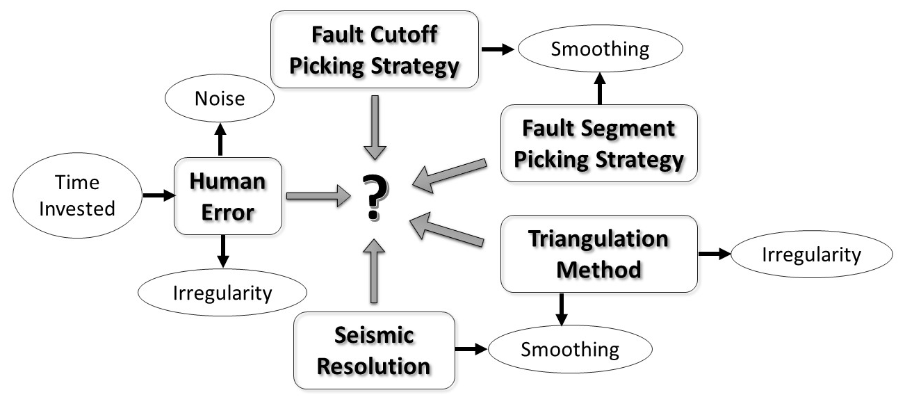
Figure 1Schematic workflow of factors that contribute to documenting the optimum picking strategy that provides the most geologically reasonable result within the shortest timeframe. Several contributing factors add noise and irregularity to fault surfaces (such as human error and triangulation method), while others act to smooth the data (such as seismic resolution, fault cutoff and segment picking strategy, and triangulation method). Finding the balance between those factors that add irregularity and those that act to smooth data is crucial.
1.1 Fault growth models
Analysing the sealing potential of faults within the subsurface is crucial, not only by using traditional methods (see Sect. 1.3) but also by use of fault growth models. How faults grow and link with other faults alters their hydraulic behaviour along fault strike. For example, areas of soft-linked relay zones can act as conduits to fluid flow (e.g. Trudgill and Cartwright, 1994; Childs et al., 1995; Peacock and Sanderson, 1994; Bense and Van Balen, 2004; Rotevatn et al., 2009). Further, an increase in deformation band and fracture intensity has been recorded at these areas of fault–fault interactions (e.g. Peacock and Sanderson, 1994; Shipton et al., 2005; Rotevatn et al., 2007), which may ultimately act to alter the hydraulic properties of the fault zone once these relay zones become hard linked. Hence, accurately capturing the geometry of faults within the subsurface is crucial to fully understand and accurately interpret how the faults have grown and hence identify areas of possible fluid flow or where high “risk” may occur.
Faults can be observed as either isolated or composite fault segments (Benedicto et al., 2003). Specifically, two principal fault growth models have been suggested: the propagating fault model (e.g. Walsh and Watterson, 1988; Cowie and Scholz, 1992a, b; Cartwright et al., 1995; Dawers and Anders, 1995; Huggins et al., 1995; Walsh et al., 2003; Jackson and Rotevatn, 2013; Rotevatn et al., 2019) and the constant-length fault model (Childs et al., 1995; Cowie, 1998; Morley et al., 1999; Walsh et al., 2002, 2003; Nicol et al., 2005, 2010; Jackson and Rotevatn, 2013; Jackson et al., 2017a; Rotevatn et al., 2018, 2019). However, other models have also been proposed, such as the constant maximum displacement length ratio model and the increasing maximum displacement length ratio model (Kim and Sanderson, 2005). The propagating fault model can be subdivided depending on whether the faults are non-coherent or coherent (Childs et al., 2017). The propagating fault model for non-coherent faults describes faults that form initially by unconnected segments that are kinematically unrelated but are aligned in the same general trend. These isolated faults propagate and link up laterally with time, progressively increasing displacement and length, forming a single larger fault with associated splays. The propagating fault model for coherent faults describes individual faults that are part of a single larger structure but are geometrically unconnected. Again, the fault propagates as the displacement increases, with new segments forming at the tip. Conversely, the constant-length model describes faults that have established their final fault trace length at an early stage, where relay formation and breaching occurred relatively rapidly and early in the evolution, after which growth occurs through increasing cumulative displacement (Childs et al., 2017). Fault propagation occurs only during linkage between segments.
Although two different models are commonly used to describe fault growth, it has recently been suggested that faults grow by a hybrid of growth behaviours (Rotevatn et al., 2019). The fault growth models are complemented by throw–distance (T-D) plots, which can be used to identify areas of fault segment linkage, often at areas of displacement lows (e.g. Cartwright et al., 1996). However, it is important to note that using T-D plots of the final fault length alone to understand fault growth may lead to ambiguous conclusions relating to which growth model best describes the evolution, in part due to the limit of seismic resolution but also due to the need for complementary analysis. Specifically, integration with growth strata is required to truly distinguish between fault growth models (Jackson et al., 2017a). This contribution focuses on T-D plots, and hence no definitive fault growth model is proposed; instead, locations of potential breached relays, and hence possible high-risk areas in terms of CO2 storage, are identified. Further, it is important to take into consideration ductile strains (e.g. folding), which can contribute to local throw minima, when conducting such analyses (Jackson et al., 2017a, b).
Faults are generally described as elliptical-shaped structures, whereby displacement is greatest in the centre of the fault, decreasing towards the tip (e.g. Walsh and Watterson, 1988; Morley et al., 1990; Peacock and Sanderson, 1991; Walsh and Watterson, 1991; Nicol et al., 1996). Through fault growth, nearby isolated faults can begin to interact, either vertically and/or laterally, leading to the formation of relay zones (Morley et al., 1990; Peacock and Sanderson, 1991). These relay zones are soft-linked structures, where the displacement maxima are not significantly influenced by the linkage. Relay zones can progress to form hard-linked structures when the relays become breached, and a common displacement maximum occurs along the length of this now-connected fault. This continues through fault evolution and can lead to fault zones where these relict relay zones are no longer obvious in map view; however, they can be identified through subtle variations in displacement along fault strike and down fault dip. However, such an analysis is highly dependent on the accuracy and detailed nature of the interpreted faults in 3-D.
It has been shown that seismic resolution controls the accuracy of the fault geometries produced, particularly when upscaling to a geocellular grid (e.g. Manzocchi et al., 2010), and sampling gaps can be caused by incorrect sampling strategies (Kim and Sanderson, 2005; Torabi and Berg, 2011), which in turn will reduce the accuracy of all fault analysis performed. Further, different seismic interpretation techniques, specifically differing seismic line spacing, will influence the resolution of the final fault surface produced and hence may cause inaccuracies when interpreting fault segmentation (Tao and Alves, 2019).
1.2 Fault seal analysis: geomechanical analysis
Understanding the sealing potential of faults in the subsurface is crucial when assessing sites for CO2 storage, especially when trying to predict the sealing behaviour of faults when fluid pressures are progressively increased during CO2 injection. Hence, analysis is required to assess whether the pressure generated by the CO2 column will cause the faults to become unstable and reactivate, causing vertical CO2 migration up the fault through dilatant micro-fracturing (e.g. Barton et al., 1995; Streit and Hillis, 2004; Rutqvist et al., 2007; Chiaramonte et al., 2008; Ferrill et al., 1999a).
Fault stability analysis requires the use of 3-D fault surface models, where the orientation and magnitude of the in situ stresses and pore pressure are used along with the predicted fault rock mechanical properties to assess the conditions under which the modelled faults may be reactivated (e.g. Ferrill et al., 1999a; Mildren et al., 2005). This method has previously been used to assess the stability of faults for CO2 storage sites in order to estimate the column of CO2 that faults can hold before reactivation may occur (e.g. Streit and Hillis, 2004; Chiarmonte et al., 2008). Since the assessment of fault reactivation potential requires an accurate 3-D fault surface model, any uncertainty generated during fault interpretation and fault surface creation through differences in sampling methodologies will be inherited by the geomechanical analysis.
1.3 Fault seal analysis: capillary seal
Methods for predicting the sealing potential of faults within siliciclastic reservoirs have received significant attention over the past few decades (e.g. Lindsay et al., 1993; Childs et al., 1997; Fristad et al., 1997; Fulljames et al., 1997; Knipe et al., 1997; Yielding et al., 1997, 2010; Yielding, 2002; Bretan et al., 2003; Færseth et al., 2006). In general, these methodologies describe a capillary seal, where surface tension forces between the hydrocarbon and water prevent the hydrocarbon phase from entering the water–wet phase; hence, the volume of hydrocarbons that can be contained by the fault is controlled by the capillary entry pressure (Smith, 1980; Jennings, 1987; Watts, 1987). The capillary entry pressure depends on the hydrocarbon–water interface (specifically the wettability, interfacial tension and radius of the hydrocarbon), the difference between the hydrocarbon-phase and water-phase densities and the acceleration of gravity. Leakage of hydrocarbons through the water–wet fault zone occurs when the difference in pressure between the hydrocarbon and water phases (the buoyancy pressure) exceeds that of capillary threshold pressure (Fulljames et al., 1997). The capillary threshold pressure is controlled by the pore throat size, which is in turn controlled by the composition of the fault rock (Yielding et al., 1997). It is important to note, however, that the differences in densities, wettability and interfacial tension that occur in CO2–water when compared to hydrocarbon–water (as is the case in this study) cause differences in capillary entry pressure and ultimately the predicted column height (Chiquet et al., 2007; Daniel and Kaldi, 2008; Bretan et al., 2011; Miocic et al., 2019; Kayolytė et al., 2020).
Where clay or shale layers are present within a succession, during faulting, these layers can either be juxtaposed against the reservoir layer or become entrained into a fault, either as a smear or as a gouge (Allan, 1989; Knipe, 1992; Lindsay et al., 1993; Yielding et al., 1997). A shale smear has been described as an abrasive shale veneer that forms a constant thickness down the fault (Lindsay et al., 1993). A fault gouge, or phyllosilicate framework fault rock (PFFR), is used to describe fault rocks that entrain clay within the fault zone, creating mixing with framework grains (Fisher and Knipe, 1998). Both mechanisms have the ability to create a barrier to fluid flow. Hence, fault seal analysis is traditionally completed by a combination of juxtaposition seal analysis, i.e. creating Allan diagrams (Allan, 1989), identifying areas where there may be communication across the fault, specifically in areas of sand–sand juxtapositions. This is then followed by a prediction of the fault rock composition by use of various industry-standard algorithms, e.g. the shale smear factor (SSF; Lindsay et al., 1993; Færseth, 2006) and the shale gouge ratio (SGR; Yielding et al., 1997). In this contribution, we focus on the SGR. This algorithm uses the proportion of clay (VClay or VShale) that has moved past a point on the fault to calculate the amount of clay within the fault rock:
where Δz is the bed thickness and VClay is the volumetric clay fraction (Yielding et al., 1997). A higher SGR generally corresponds to an increase in phyllosilicates entrained into the fault (e.g. Foxford et al., 1998; Yielding, 2002; van der Zee and Urai, 2005). Hence, a higher capillary threshold pressure is likely, which is predicted to retain a higher hydrocarbon column held back by the fault (e.g. Yielding et al., 2010). Hence, the next step in a fault seal analysis workflow is to predict the column that can be held back by the fault (e.g. Sperrevik et al., 2002; Bretan et al., 2003; Yielding et al., 2010). For applicability in CO2 storage, these calibrations would need to be altered to take into consideration the different densities, wettability and interfacial tension (Bretan et al., 2011; Miocic et al., 2019; Kayolytė et al., 2020). However, for simplicity, this paper focuses on how interpretation influences the juxtaposition of sand bodies and calculated SGR, rather attempting to predict any column heights, due to the implicit uncertainties that are imposed by the CO2–water–rock systems.
The Smeaheia site (see Mulrooney et al., 2020, and references therein) is located approximately 40 km northwest of the Kollsnes processing plant, and around 20 km east of Troll East, in the northern Horda Platform (Fig. 2). The northern Horda Platform is a 300 km by 100 km, N–S elongated structural high along the eastern margin of the northern North Sea (Færseth, 1996; Whipp et al., 2014; Duffy et al., 2015; Mulrooney et al., 2020; Fig. 2). Many deep-seated, west-dipping basement faults occur within the Horda Platform, generating several half-graben bounding fault systems with kilometre-scale throws (Badley et al., 1988; Yielding et al., 1991; Færseth 1996; Bell et al., 2014; Whipp et al., 2014).
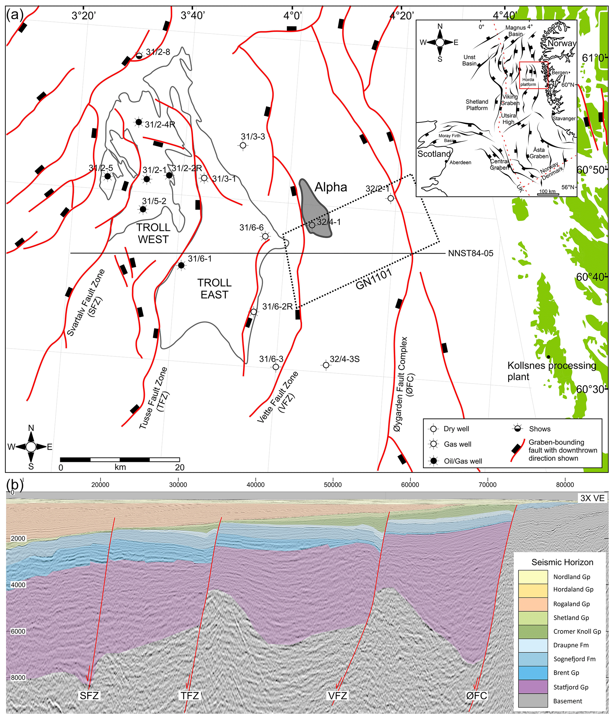
Figure 2(a) Location of the Smeaheia site within the Horda platform, indicated by the Alpha prospect, partially covering the GN1101 survey. Graben-bounding faulting is shown, along with the hydrocarbon discovery of the Troll field. The 3-D survey used in the analysis is outlined by a dashed black line: GN1101. Wells used in the analysis are shown. Norwegian license blocks are shown. The Norwegian coastline outlined in green with the Kollsnes processing plant highlighted for reference, modified from Norwegian Petroleum Directorate Fact Maps (http://factmaps.npd.no/factmaps/3_0/, last access: July 2020). Inset: location of the Horda Platform in relation to the North Sea, Norwegian and Scottish coastline. Main structural elements are shown, such as basin-bounding faults, main basins and structural highs. After Mulrooney et al. (2020). (b) Regional cross section across the northern Horda Platform, from 2-D seismic NNST84-05, the location of the seismic section marked in panel (a).
Two first-order, thick-skinned faults occur within the Smeaheia site: the VFZ and the Øygarden Fault Complex (ØFC) (Fig. 2), which bound an east-tilting half graben following a roughly north–south trend. The focus of this study is the VFZ, bounding the gently dipping three-way closure Alpha prospect in its footwall (Figs. 2, 3). It is located 20 km to the east of the Tusse Fault: a half-graben bounding, sealing fault allowing for the accumulation of hydrocarbons in Troll East.
Smaller-scale, thin-skinned northwest–southeast-striking faults are also recorded at the Smeaheia site (Mulrooney et al., 2020). These faults only affect post-Upper Triassic stratigraphy and have low throws of less than 100 m (Fig. 3). These faults are associated with Jurassic to Cretaceous rifting, which also caused reactivation of the Permo-Triassic basement-involved faults (Færseth et al., 1995; Deng et al., 2017). However, these smaller-scale faults are not the focus of this study.
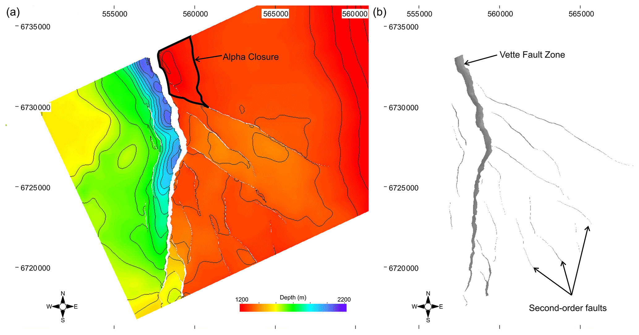
Figure 3(a) Depth structure map of the top Sognefjord Formation. (b) Fault heave map of the top Sognefjord Formation.
This study focuses on the Sognefjord and Fensfjord formations as storage reservoirs for CO2 (Figs. 3, 4). Both units lie within the middle–upper Jurassic Viking Group. These units represent stacked saline aquifers at this location. They are composed of coastal to shallow marine deposits dominated by sandstones with finer-grained interlayers (Dreyer et al., 2005; Holgate et al., 2013; Patruno et al., 2015). Of these, the Sognefjord Formation at the top of the stacked aquifer offers the best properties. It occurs at approximately 1200 m depth in the Alpha prospect and has a permeability of 440–4000 mD and a porosity of 30 %–39 % (Statoil, 2016; Ringrose et al., 2017; Mondol et al., 2018). The Sognefjord Formation is capped by deep marine, organic-rich mudstones of the Draupne Formation, as well as deep water marls, carbonates and shaley units in the Cromer Knoll and Shetland groups above the base Cretaceous unconformity (Nybakken and Bäckstrøm, 1989; Isaksen and Ledjie, 2001; Kyrkjebø et al., 2004; Justwan and Dahl, 2005; Gradstein and Waters, 2016; Fig. 4).
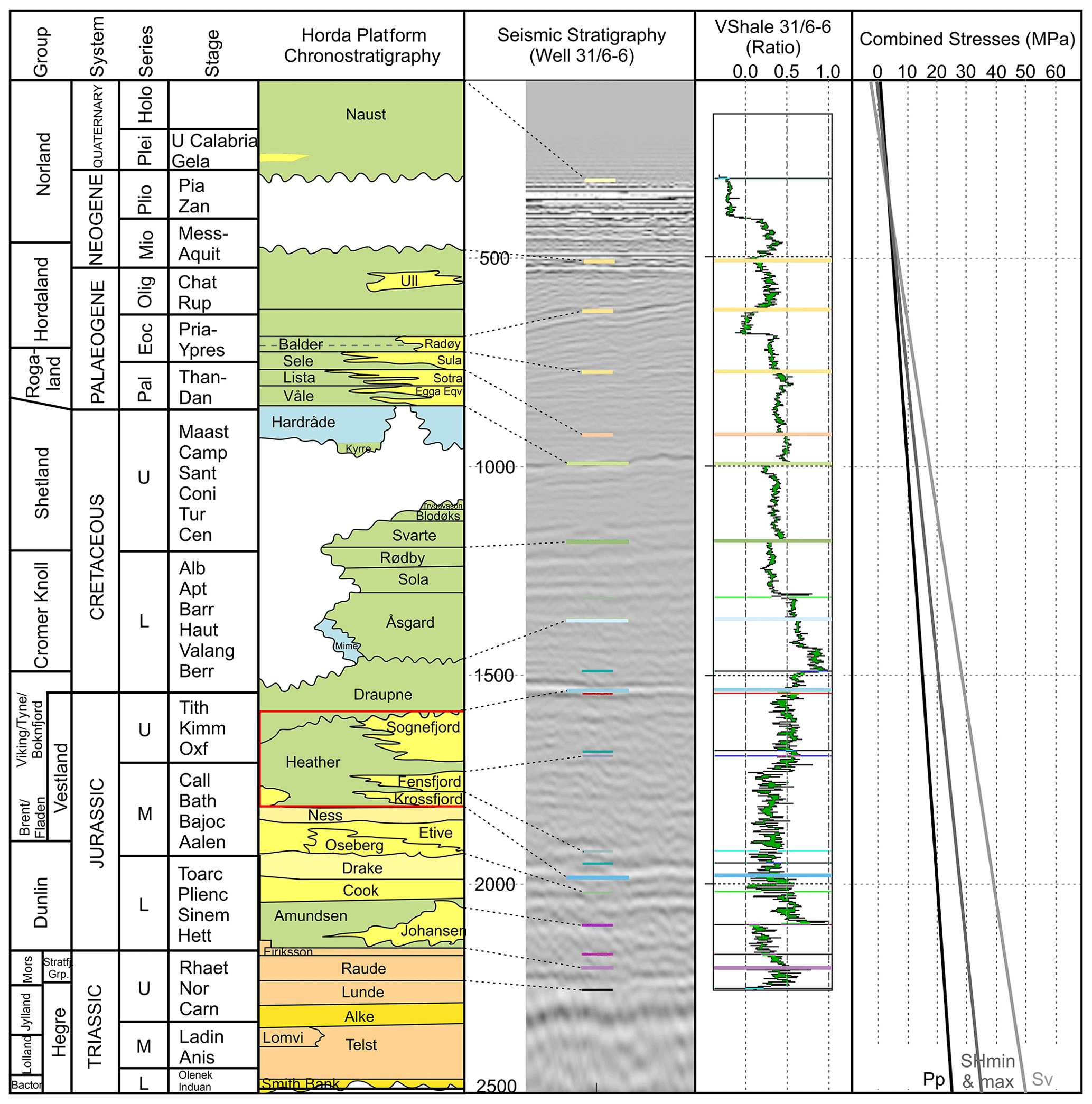
Figure 4Lithostratigraphic chart of the Horda Platform from Halland et al. (2011), with the area of interest highlighted in the red box: the Sognefjord, Fensfjord and Krossjord formations. A seismic section is shown intersecting well 31/6-6 within the survey SG9202. Marker horizons are shown corresponding to the lithostratigraphic column. The VShale curve from well 31/6-6 is shown, with marker horizons for reference. The in situ stress field is shown using the combined stresses (in MPa). Pp: pore pressure. SHmin: minimum horizontal stress. SHmax: maximum horizontal stress. Sv: vertical stress. Seismic stratigraphic column, VShale and combined stress field all have the same depth range.
The Alpha prospect has been drilled for exploration purposes, due to hypothesized hydrocarbon migration scenarios, into the Smeaheia site (Goldsmith, 2000); however, well data from the Alpha prospect (32/4-1) have recorded no oil shows, indicating that no hydrocarbon migration has occurred into the Smeaheia site (32/4-1 T2 final well report 1997). As a result, the Smeaheia site has been assessed for the potential for CO2 storage in a saline aquifer, as it fulfils requirements for substantial datasets, minimal influence on nearby production sites and proximity to infrastructure.
Faults and horizons have been interpreted using one main 3-D survey: GN1101, covering the Smeaheia area (Fig. 2). However, it is important to note that this survey does not extend far enough to the north and south to interpret the entire fault structure of the VFZ. Hence, only the section of fault that is observed in the GN1101 survey is analysed. The GN1101 3-D survey is a time-migrated dataset that has subsequently been depth-converted using a simple velocity model that has been created using quality-controlled time–depth curves from 15 wells from the Troll and Smeaheia area: 31/2-1, 31/2-2R, 31/2-4R, 31/2-5, 31/2-8, 31/3-1, 31/3-3, 31/5-2, 31/6-1, 31/6-2R, 31/6-3, 31/6-6, 32/2-1, 32/4-1 T2 and 32/4-3 S (Fig. 2). Other wells in the area have no velocity data. The GN1101 survey has good seismic quality with a resolution of roughly 15.75 m at the Sognefjord level, suitable for detailed structural interpretation. The GN1101 survey was shot in 2011 by Gassnova SF, with an inline spacing of 25 m and a crossline spacing of 12.5 m, covering an area of 442.25 km2. Crosslines are oriented 065∘, and inlines are oriented 155∘. GN1101 has normal polarity and a zero-phase wavelet.
Five seismic horizons have been interpreted: top–Shetland Group, top–Cromer Knoll Group, top–Draupne Formation, top–Sognefjord Formation and top–Brent Group. The aforementioned wells with quality-controlled (QC) time–depth curves used for depth conversion have been used to aid seismic interpretation by use of well pick locations (Fig. 4).
The VFZ has been interpreted using different line spacing in order to assess the optimum picking methodology. Faults have been picked every 1, 2, 4, 8, 16 and 32 lines, corresponding to 25, 50, 100, 200, 400 and 800 m spacing, respectively. Rigorous QC has been performed to ensure all data points honour the fault surface precisely and to maintain continuity of the fault location between each inline. Note that, since the GN1101 survey has been shot orthogonally to the VFZ strike trend (as is often the case, where surveys are shot perpendicular to the main fault trend to best capture their nature), only the inline orientation has been picked within this assessment. Adding crosslines would simply add increased noise due to the significant picking uncertainty when a fault is parallel to the seismic line, causing mismatches between the interpretation on inlines and crosslines. Time slices using a variance cube have also been utilized to guide interpretation, as these often provide an improved visual representation of the precise location of the fault. Seismic processing focused on resolving the Jurassic interval; as such, the seismic quality is excellent at this location but can be significantly more noisy elsewhere. Hence, interpreting on time slices alone would lead to huge ambiguity, and thus they are used for interpretation guidance only.
Interpretation and fault surface generation were performed using the software T7. The fault surfaces have been created using different algorithms, illustrated in Fig. 5: (1) unconstrained triangulation, (2) constrained triangulation and (3) gridded. A combination of equant and irregular triangles of difference sizes, reflecting the picking strategy, has also been used for each triangulation algorithm. Unconstrained triangulation generates a fault surface that triangulates fault segments without constraining the surface to conform to the lines between adjacent points on the same fault segment but honouring all picked points. Constrained triangulation generates a surface that conforms to the points and the lines between adjacent points on the same fault segment. Both unconstrained and constrained triangulations honour all data points, and the number of data points on all fault segments controls the number of triangles. Gridded modelling strategy consists of regularly sampled points with a grid cell dimension varying with distance between the interpreted seismic lines; hence, grid cell dimensions vary with sampling strategy. Note that no further smoothing has been applied to any of these modelling strategies. Unconstrained triangulation is the main algorithm shown throughout, as this offers a “middle-ground” modelling strategy, honouring data points but allowing some smoothing of the surface. However, the influence of algorithm choice is also assessed on any subsequent fault analysis, specifically fault dip.

Figure 5An example of arbitrary fault segments picked at a spacing of 250 m (every 10th line), showing how different triangulation methods produce differing fault surfaces. This has been done for non-equant and equant triangles (at a size of 250 m) for constrained and unconstrained triangulation, as well as gridded methods. Fault segments are shown in red, while the triangulated surfaces are shown by black lines. How these triangulation methods strike along the fault is shown (non-equant triangles), next to the picked fault segments, indicating how much smoothing is added. Constrained triangulation honours all data points and adjacent segments, adding more irregularity to the fault surface. The gridded algorithm creates a surface that consists of regularly sampled points. Note that in this example, the smoothing and irregularity of the fault surface are subtle due to the wide spacing of the fault segments; narrower spacing leads to increased irregularity.
Fault attributes are calculated and mapped onto the fault surface at a resolution of 8 m lateral by 4 m vertical, providing an optimum seismic resolution without the need to extend processing time. The aforementioned methods of fault surface generation are used to assess the differences in fault strike, dip and geomechanical attributes, when analysing fault growth and fault stability. Further, fault cutoffs (intersection lines on the fault surface highlighting horizon–fault cutoffs) have been picked at each of the six fault surface iterations, for the five mapped seismic horizons, again using different line spacing to aid with cutoff picking. Fault cutoffs have been picked using a combination of seismic slicing, at a distance of 10 m into the footwall and hanging wall of the fault to remove any seismic noise, as well as using inlines at different line spacing to accurately assess where the horizons intersect the fault (example shown in Fig. 6). The line spacing used is the same as that for interpreting the fault segments; for example, a fault interpreted on every eight lines (200 m spacing) also uses inlines at 200 m spacing to aid with picking the cutoffs. These fault cutoffs are used to calculate fault throw, which is mapped onto the 3-D fault surfaces, and to produce T-D plots used to analyse fault growth. Complications arise when picking fault cutoffs due to significant drag in the hanging wall of the VFZ. Fault cutoffs have been picked honouring the drag (Fig. 6a, crosses) in order to accurately capture the juxtapositions, as well as removing the drag (Fig. 6a, circles), in order to accurately interpret fault growth (see Jackson et al., 2017a, b).
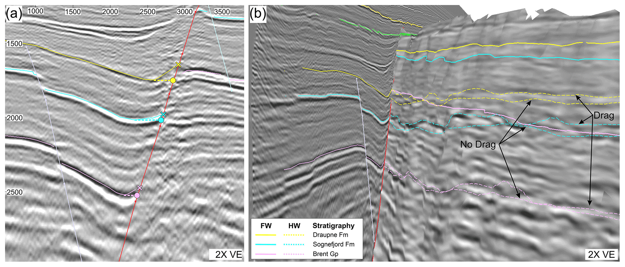
Figure 6(a) Inline 1224 from the GN1101 survey showing how two different fault cutoffs are created: with and without incorporating drag. Fault cutoffs including drag simply model where the drag intersects the faults, as shown by the X on the faults for the Draupne Fm. (yellow), Sognefjord Fm. (blue) and Brent Gp. (pink) horizons. Fault cutoffs are modelled with no drag by observing the lowest point in the hanging wall syncline and extrapolating this point perpendicularly to the fault plane, as indicated by the dashed horizontal lines and the circles at the intersections. (b) Oblique view of inline 1224 and the fault surface showing the footwall (FW) (solid line) and hanging wall (HW) cutoffs (dashed lines). The two iterations of the HW cutoffs show the difference between incorporating drag and modelling the fault cutoffs with no drag. The fault surface shows the seismic slice from 10 m into the hanging wall.
We assessed the differences in fault stability between each picking strategy. This is crucial when considering how the pressure increase due to CO2 injection may influence the reactivation potential of any bounding or intra-basin faults. In situ stress data have been derived from an internal Equinor data package (unpublished), using data from four nearby wells: 31/6-3, 31/6-6, 32/4-1 and 32/2-1. Vertical stress (Sv) was determined from the overburden gradient. The minimum horizontal stress (SHmin) was determined from extended leak-off tests and the pore pressure (Pp) is measured as being hydrostatic. The maximum horizontal stress (SHmax) is assumed to be the same as SHmin, using data documenting the stress orientation and faulting regime based on exploration and production wells. This area of the northern North Sea is found to be within a normal faulting regime with almost isotropic horizontal stresses at shallower (<5 km) levels (Hillis and Nelson, 2005; Andrews et al., 2016; Skurtveit et al., 2018). The orientation for SHmax is likely to be trending E–W, based on borehole breakout data (Brudy and Kjørholt, 2001; Skurtveit et al., 2018). The in situ stress regime is summarized in Fig. 4 and Table 1. The cohesion used for this study has been set as 0.5 MPa and the frictional coefficient as 0.45. These values have been chosen based on the modelled SGR where the Sognefjord Formation is observed in the footwall. Values of approximately 40 % SGR have been calculated (see Sect. 4.2), which has been used to estimate the cohesion and frictional coefficient values based on previously published values (Meng et al., 2016, and references therein). Results of slip tendency, dilation tendency and fracture stability are shown within this paper. Slip tendency is the ratio of resolved shear stress (τ) to normal stress (σn) on a plane, where the higher the value, the more likely the fault will slip by shear failure (Morris et al., 1996). Shear failure will generally occur at approximately 0.6, which is the coefficient of static friction. However, it is important to note that the coefficient of static friction is unknown in this scenario. The likelihood of the fault to slip depends on the stress field and orientation and/or dip of the fault surface. Dilation tendency is the relative probability of a plane to dilate within the current stress field (Ferrill et al., 1999b). This is a ratio between 0 and 1, where the higher the value, the more likely a fault will go into tensile failure. Fracture stability (FAST) estimates the pore pressure required to reduce stresses that forces a fault into either shear or extensional failure (Mildren et al., 2005). Both dilation tendency and fracture stability take into consideration the cohesion and tensile strength of the fault rock.

How the picking strategies may influence fault seal analysis by means of juxtaposition diagrams (Allan, 1989) and calculated SGR (Yielding et al., 1997), has also been analysed. A gamma-ray log from nearby well 31/6-6 (Fig. 2) has been converted into VShale (Fig. 4), using a simple transform approach, where 100 % VShale is assigned to the maximum average gamma-ray value and 0 % VShale is assigned to the minimum average gamma-ray value, with a linear relationship between these being assumed (e.g. Rider, 2000; Lyon et al., 2005). Note that only one well with one VShale log that had not gone through QC, using the cursory gamma ray to VShale transform, has been used, simply as a proxy to identify how picking strategies may influence the overall fault seal analysis, rather than to perform any rigorous fault seal analysis. If the same VShale curve is used for all instances, then any differences identified in each scenario is simply a product of the picking strategy used. The VShale is draped onto the fault, using the locations of picked fault cutoffs, which tie with well picks, and is used along with the throw to calculate the SGR along the 3-D fault surface.
Note that all seismic interpretation, fault surface creation and subsequent fault analysis was performed using the software T7. Complications may arise when transferring data between different software packages. However, this added complication has not been addressed within this contribution.
4.1 Fault segmentation analysis
Two main attributes are used to aid predictions of how the faults have grown on the seismic scale: throw profiles and strike variations. Sudden changes in throw and fault strike may indicate where initially isolated seismic-scale fault array segments subsequently linked (e.g. Cartwright et al., 1996). It is important to note, however, that not all changes in fault strike may be caused by fault linkage, and not all fault linkage will result in a change in fault strike. Hence, analysis using a combination of these fault attributes improves our understanding of the seismic-scale fault growth history. Moreover, this analysis cannot perform fault growth analysis for any fault segmentation that is below seismic resolution, i.e. early in the fault growth phases.
4.1.1 Throw profiles
Throw profiles highlight areas where the current fault surface was once segmented. Here, we show throw profiles for the top Sognefjord along the VFZ (Fig. 7). We can observe that the location, nature of fault interactions and number of segments within initial fault array varies with picking strategy (Fig. 7). Picking every line (25 m spacing) is the finest resolution in this example and is assumed to provide the best picking strategy to identify all areas of seismic-scale fault segmentation. Using every line, we can interpret seven fault segments, identified by six areas of breached relays (Fig. 7, highlighted by dashed vertical lines). Areas of breached relays are interpreted where significant drops in throw are observed, varying from the overall throw profile and are not interpreted to be caused by other currently intersecting faults. Increasing the picking spacing decreases the detail required for accurate fault growth analysis. However, we can observe that increasing the spacing to 100 m retains the level of detail needed to identify all fault segments within this study, that are also identified using every line spacing (Fig. 7a vs. Fig. 7c). Beyond this spacing, the level of detail is decreased causing the ability to identify some fault segmentation to be lost. This is most pronounced when the area of fault–fault intersection, and hence change in throw amplitude, is subtle. This can be observed in Fig. 7d, where a picking spacing of 200 m loses the segmentation interpreted at approximately 1375 m, due to the low throw variation (c. 25 m throw amplitude) at this location. Using 400 and 800 m picking spacing loses significant detail, such that identification of fault segments is not possible for all cases where fault interactions caused throw variations of lower than 75 m (Fig. 7e and f). Further, the precise location of interpreted fault segmentation is often incorrect, such as that identified at 3000 m, which should in fact be two areas of separate fault–fault intersections (Fig. 7e and f).
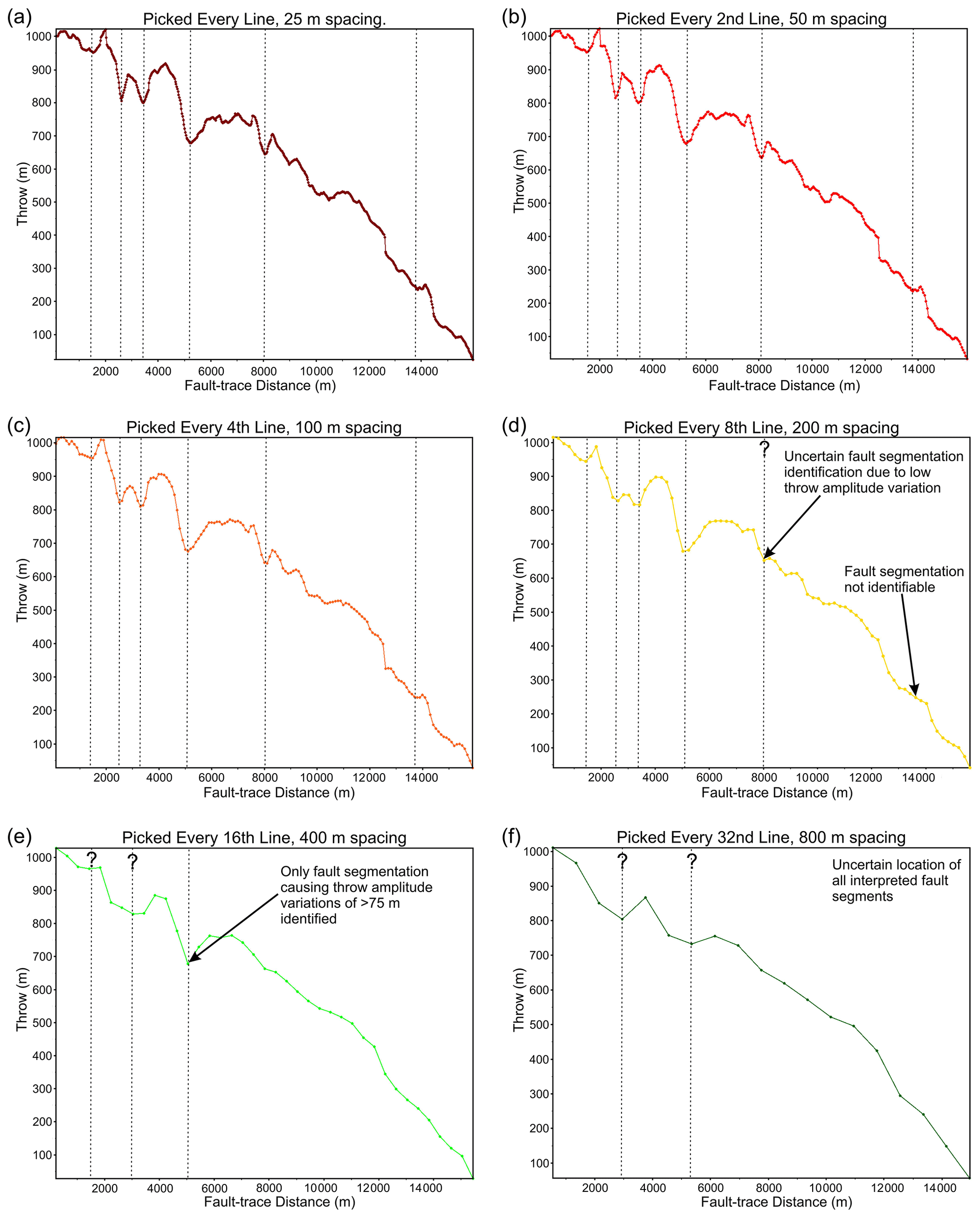
Figure 7Fault throw–distance plots at the top Sognefjord for each picking strategy: 25, 50, 100, 200, 400 and 800 m line spacing. Location of fault segmentation identified by changes in throw along strike is highlighted using dashed vertical lines. Those that are uncertain are indicated using a question mark. Picking using every line generates an accurate throw profile, indicating seven fault segments that occur within the GN1101 survey extents. This is also shown using a spacing of 50 and 100 m. Location and number of fault segments become increasingly uncertain when the spacing increases beyond 100 m.
To provide more detail, we show how two picking strategies compare by normalizing the distance along the fault (Fig. 8, top) and by showing fault throw attributes and contours on the triangulated fault surfaces (Fig. 8, bottom). Since the widest spacing that can be used without losing any segmentation detail is 100 m, we compare this example with the throw profile generated by picking every 800 m line spacing (Fig. 8). We have highlighted four localities along the fault where fault segmentation is observed on the narrower line spacing, showing displacement minima, and compared this to a displacement profile that does not show these displacement minima when picked using a coarser line spacing (Fig. 8, black circles). Hence, the locations for fault segmentation are missed when a coarser line spacing is picked.
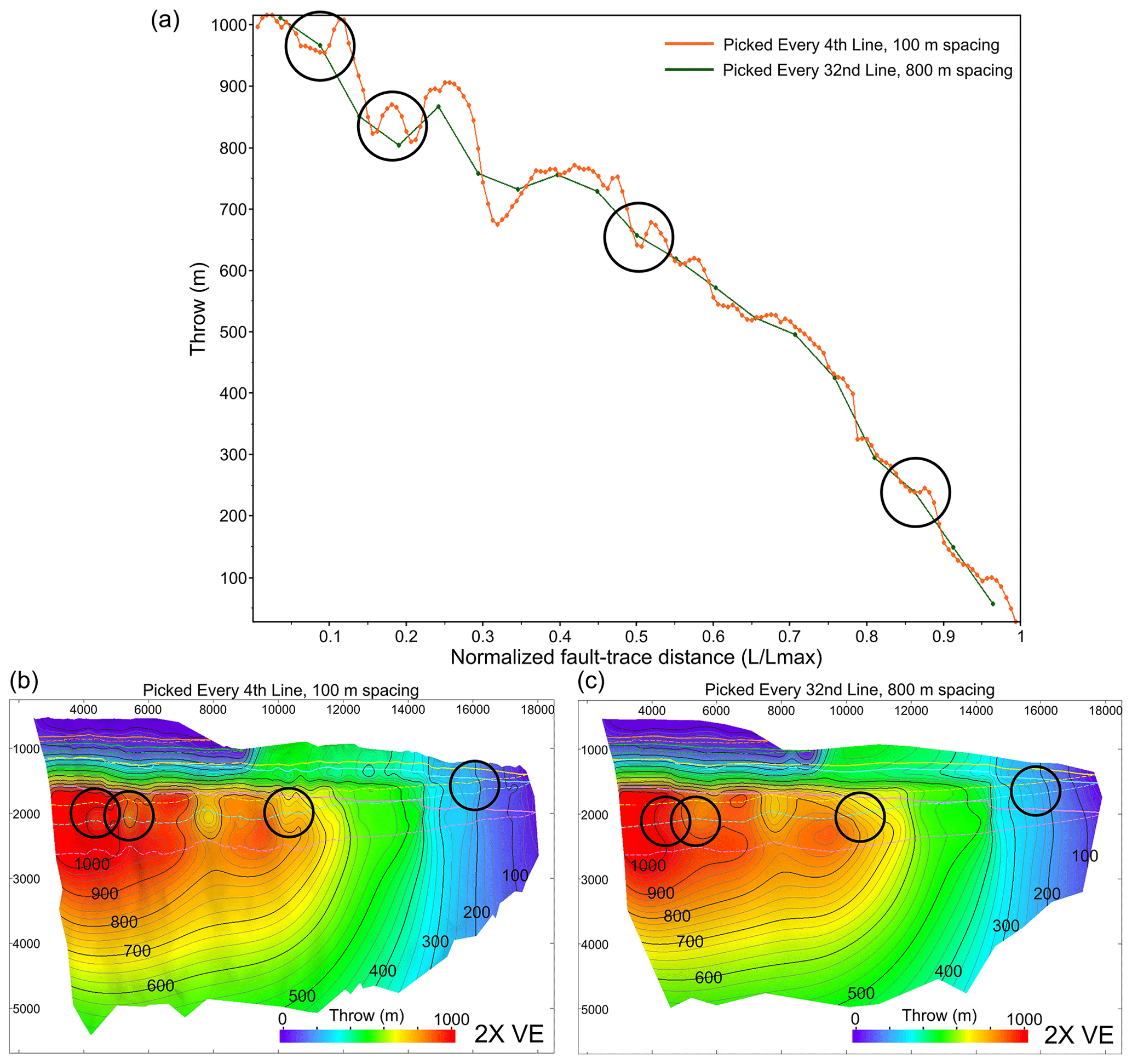
Figure 8(a) Fault throw–distance profile for the Vette fault picked at a spacing of 100 and 800 m. The x axis has been normalized for distance along fault trace (length length max) in order to directly compare the two scenarios. The T-D plots have been normalized due to the restrictive size of the GN1101 survey, meaning that faults picked at increasing line spacing increments will be slightly shorter than the last. Bottom: contoured fault throw plots displaced on a fault surface picked at every 100 m line spacing (b) and 800 m line spacing (c). Circles highlighted in the throw–distance graph correspond to the same circles highlighted on the fault throw plots. We can observe the four fault segments that are not recorded when a picking strategy of 800 m line spacing is used. These fault segments are recorded in the throw profile when a narrower spacing strategy is used but are smoothed out and lost when a wider spacing strategy is used. Note that unconstrained triangulation is used for fault surface generation.
4.1.2 Strike
Through examination of strike variations along the fault surface, we can see a sudden change in principal strike direction shown at roughly 9000 m from the north in the fault plane diagrams in Fig. 9. The strike changes from approximately 320 to 360∘ in the north to approximately 000 to 025∘ in the south. Further, corrugations are observed along fault strike, which may be associated with fault segmentation (e.g. Ferrill et al., 1999b; Ziesch et al., 2017). However, variation in this strike trend occurs with differing picking strategies, as well as the total number of corrugations. Although the significant change in trend observed at 9000 m in all fault plane diagrams from the north exists regardless of picking strategy, faults that are picked at 25 and 50 m line spacing create highly irregular surfaces, where significant strike variability is observed over relatively short distances. While this is also observed for fault surfaces picked at 100 and 200 m line spacing, the irregularity of the surfaces is considerably less. However, using widely spaced picking strategies, i.e. 400 and 800 m line spacing, led to smoothing of the overall fault structure. Although the sudden change in strike observed at roughly 9000 m from the north remains, finer detail to strike variation is lost. It is this detail that is important when interpreting how the faults have grown by fault–fault interaction and hence identifying areas that may impact fluid flow will be lost. Further, the range of strike is reduced when wider spacing is used. For example, when 800 m line spacing is used for seismic interpretation, the range of fault strike only varies over 20∘, from 330 to 350∘, in the north, and 10∘, from 000 to 010∘, in the south. Conversely, when every line is used for seismic interpretation, the range of fault strike varies over 40∘, from 320 to 360∘, in the north and over 30∘, from 355 to 025∘, in the south (Fig. 10c vs. Fig. 10a). This decrease in strike range with increased line spacing may limit the interpretation of fault growth.
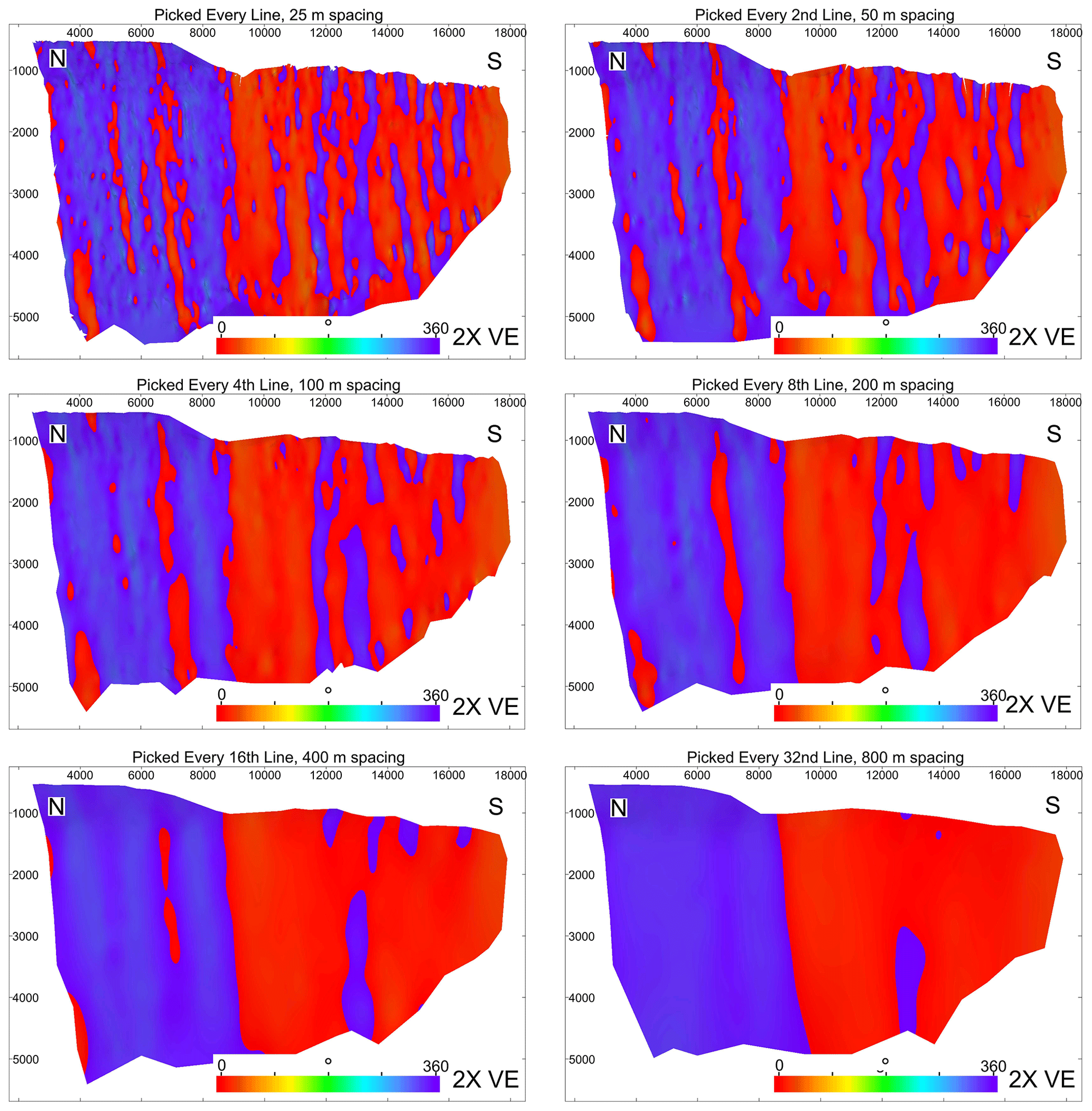
Figure 9Fault plane diagrams showing fault strike attributes displayed on the fault surfaces for each picking strategy: 25, 50, 100, 200, 400 and 800 m line spacing. Fault strike is observed to vary with line spacing used for fault picking. A highly irregular fault surface is observed when every line is used for picking, when compared to the overly smooth surface when a line spacing of 800 m is used for picking. Note that unconstrained triangulation is used for fault surface generation.
To assess the influence of fault segmentation on fault strike, we have highlighted the location of interpreted seismic-scale fault segmentation, using T-D plots, on the fault surfaces showing strike attributes (Fig. 10). We can see that when a fault surface is picked using every line, a highly irregular surface is created with highly variable orientations, and not every observed corrugation correlates with a displacement minimum on the throw profile (Fig. 10a). Conversely, when a fault surface is picked using 800 m line spacing, the surface becomes overly smoothed, where no corrugations are shown where fault segmentation is identified on the T-D plot. However, when every 100 m line spacing is used for fault picking, it appears that the majority of fault segments are also identified by fault corrugations, particularly within the northern part of the fault (Fig. 10b). However, some picked segmentations using T-D plots are not identified using corrugations, likely because not all areas of fault linkage cause a change in fault strike. Further, towards the southern half of the fault, corrugations are observed that do not correlate with fault segments picked using T-D plots. While this may indicate that an overly irregular fault surface may have been created through human error or triangulation method, it may also highlight potential areas of fault segmentation that cannot be identified by using T-D plots alone. Alternatively, corrugations could be a product of faulting within brittle and/or ductile sequences, where different types of failure within this sequence can create fault bends with abandoned tips or splays due to strain localization and not necessarily indicate initially isolated fault segments (Schöpfer et al., 2006). Further, the corrugation size (small strike dimensions but large dip dimensions) may indicate potentially implausibly low aspect ratios (see Nicol et al., 1996), and faults are generally recorded as decreasing in roughness with displacement (Sagy et al., 2007; Brodsky et al., 2011); hence, other causes for the corrugation creation may also need to be considered.
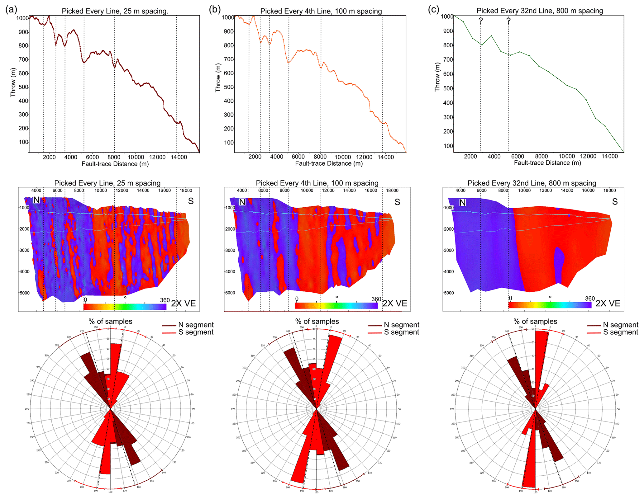
Figure 10T-D plots, fault plane diagrams showing strike and rose diagrams for scenarios picked at a line spacing of 25 m (a), 100 m (b) and 800 m (c). Areas where fault segmentation has been picked using the T-D plots have been extrapolated onto the fault plane diagrams in order to assess whether areas of strike irregularities are fault corrugations highlighting areas of segmentation. Blue lines on fault plane diagrams show the level of the top Sognefjord as HW (thicker lines) and FW (thinner lines) cutoffs. Rose diagrams illustrating the orientation and range of orientation for each scenario. Note that unconstrained triangulation is used for fault surface generation.
4.2 Shale gouge ratio modelling
The calculated SGR is not observed to vary substantially with picking strategy for this case study (Fig. 11a, b), even though substantial changes to the fault throw along strike are observed (Fig. 11e), associated with differences in picking strategies (as described above). Hence, the predicted shale content within the fault does not appear to vary significantly due to picking strategy. The shale content when a 25 m line spacing is used is estimated to be around 40 %–50 % SGR (high SGR values) within the Sognefjord Formation in the footwall (Fig. 11a). The same SGR values are also calculated when the fault segments and fault cutoffs are picked using every 800 m line spacing, despite large areas of drag being missed (Fig. 11b).
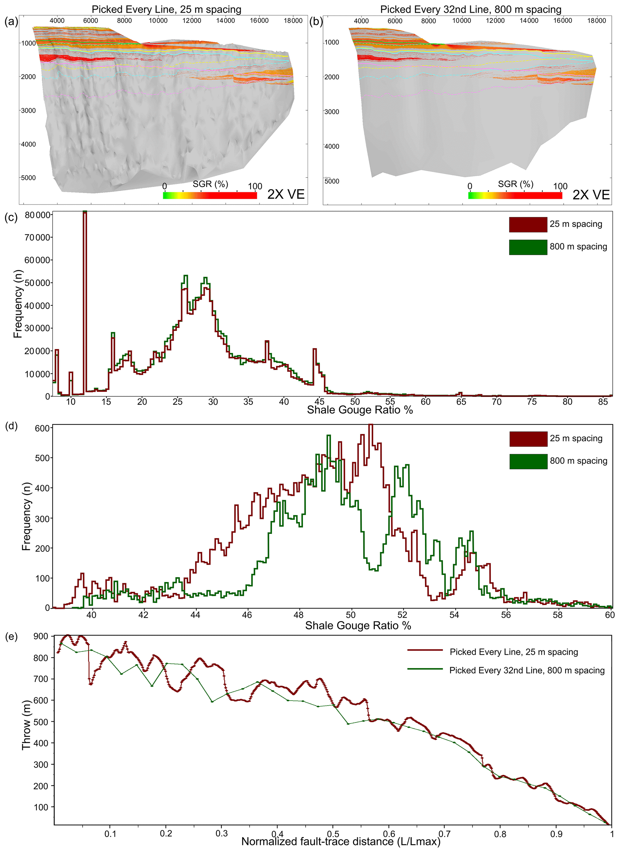
Figure 11Influence of picking strategy on the predicted SGR. (a, b) Fault plane diagrams showing the predicted SGR at low VShale (<0.4) overlaps (sand–sand juxtapositions) along the fault, when a 25 m picking spacing is used (a) and when an 800 m picking spacing is used (b). (c, d) Histograms showing the frequency of SGR for different picking strategies; dark red: 25 m spacing, green: 800 m spacing. (c) Histogram for predicted SGR along the entire fault surface. (d) Histogram for predicted SGR at low VShale overlaps within the juxtaposed Sognefjord Formation in the footwall. (e) Throw–distance plot for fault cutoffs picked every 25 m (dark red) and 800 m (green). Note that the distance has been normalized.
When we examine the frequency of SGR values across the entire fault surface, we can observe that there are only minor discrepancies between using a 25 and 800 m spacing picking strategy (Fig. 11c). However, when we take a closer look at the frequency of SGR values where only the Sognefjord Formation is juxtaposed in the footwall and only those values where low VShale values (<0.4) are juxtaposed (i.e. at sand–sand juxtapositions), we can see slight differences between the picking strategies, despite the overall high SGR values. When every 800 m is picked, the SGR is generally higher at these localities compared to when every line is picked. However, the shale content in the fault may in fact be less, as the calculated SGR is lower when 25 m line spacing is used for fault cutoff modelling, which takes into consideration all areas of drag (Fig. 11d).
4.3 Geomechanical modelling
Although the predicted fault stability is influenced by external factors, specifically the in situ stress conditions, it is also heavily influenced by intrinsic fault attributes, namely strike and dip. Since the stress conditions used in this study are isotropic, fault dip has a primary control on fault stability over fault strike. Here, we show how fault dip, and hence geomechanical analysis, varies with picking strategy.
4.3.1 Dip
Fault dip varies down the VFZ. There is low fault dip within the top 1000 m, particularly in the northern section, where the fault penetrates younger stratigraphy, specifically the Cromer Knoll and the Shetland groups. Here, the dip decreases to approximately 35∘ but can be as low as 15∘ at the very top of the fault (Fig. 12). The fault then steepens in dip to approximately 70∘ at 1500–4000 m depth, beyond which the dip decreases again to approximately 40∘ at the base of the fault.
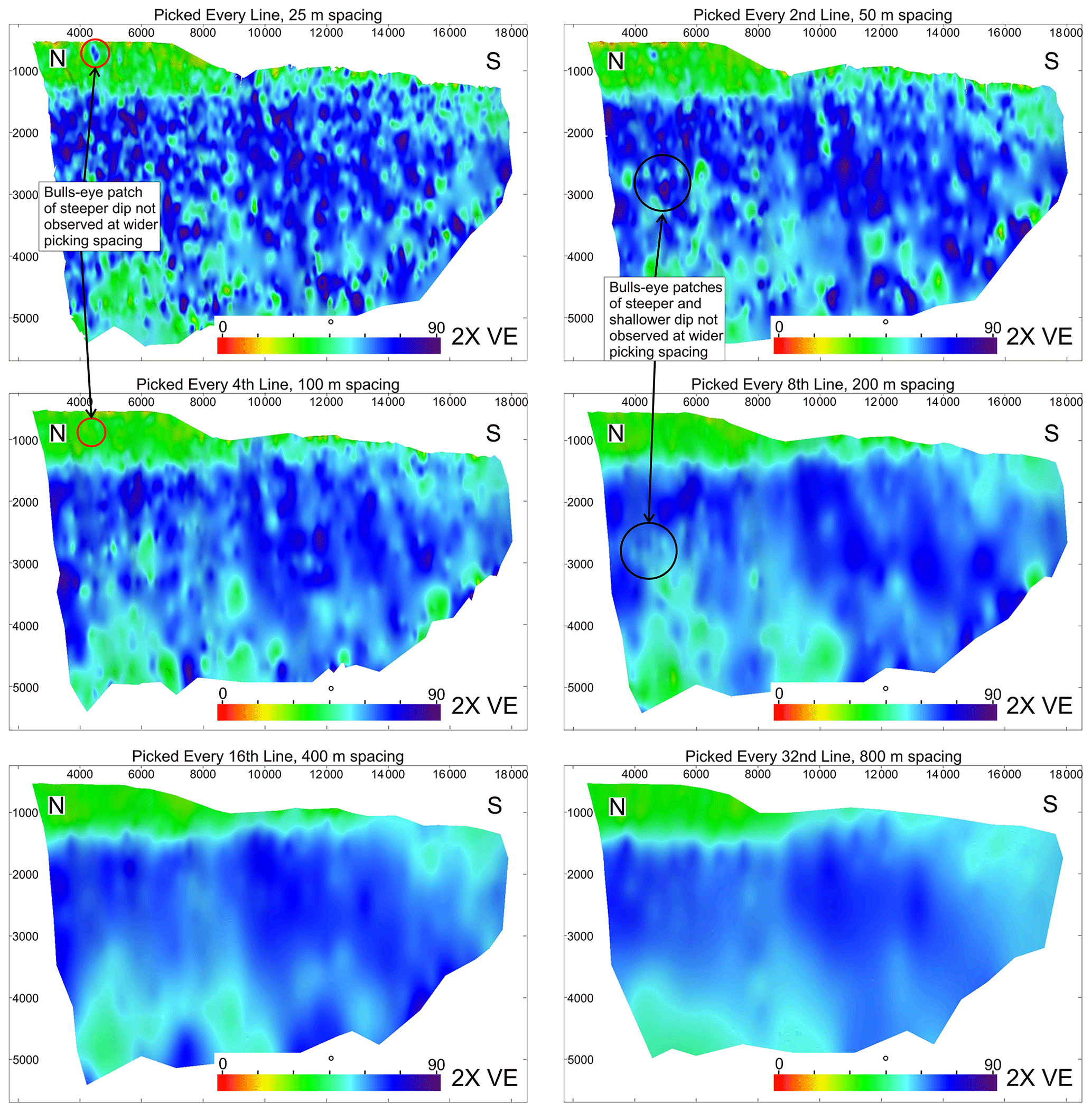
Figure 12Fault plane diagrams showing fault dip attribute displayed on the fault surfaces for each picking strategy: 25, 50, 100, 200, 400 and 800 m line spacing. Fault dip is observed to vary with line spacing used for fault picking. A highly irregular fault surface is observed when every line is used for picking, when compared to the overly smooth surface when a line spacing of 800 m is used for picking. Note that unconstrained triangulation is used for fault surface generation.
Similar to fault strike, fault dip also varies according to picking strategies. The shallowly dipping portion at the top of the fault is smoothed with increasing picking spacing, such that the lowest dip for fault surfaces picked at every 400 and 800 m line spacing is 35∘, compared with 15∘ dip for faults picked at every 25 and 50 m line spacing. Further, small bulls-eye areas of steeper dip are also removed and smoothed when picking strategy is increased (Fig. 12, red circles). Similarly, the steeper portion of the fault is smoothed as the line spacing used for picking is increased. This decreases the range of dips and smooths any bulls-eye patches of steeper or shallower dip (Fig. 12, black circles).
Although rigorous QC has been performed to improve continuity between each inline, there remains several places where slight differences in picking have occurred between lines. This human error leads to an increased irregularity of the fault surface, often creating these bulls-eye areas of inconsistent dip, associated with the triangulation algorithm trying to honour each point along the fault segments. These bulls-eye patches are roughly 100–200 m in size and generally occur at and below the Sognefjord level. Since fault stability is influenced by fault dip, these areas will be brought through to geomechanical modelling. The uneven nature of the fault surface is most severe when every inline line has been picked (e.g. Figs. 11a and 12). The irregularity decreases with increased picking spacing.
4.3.2 Fault stability
Dip varies with picking strategy, as does the predicted fault stability (Fig. 13). Along fault strike, there are minor patches where the fault is predicted to be more stable (i.e. low dilation tendency and slip tendency values or high fracture stability values) than the surrounding values and patches where the fault is predicted to be less stable. These patches are most apparent when every line is picked, with irregularity decreasing in severity until every 100 to 200 m line spacing is used for picking, where the frequency of these irregular patches is reduced. Since the fault surface is smoothed with greater picking spacing (i.e. >200 m line spacing), the results for fault stability are also smoothed, reducing the range of values for each algorithms used (Fig. 14). Hence, interpretation of fault stability will vary with picking strategy and may in fact lead to unlikely fault stability assumptions. For example, areas where the fault is predicted to be close to failure are only observed in this study when a narrower picking strategy is used (Figs. 12, 13). These areas are smoothed out and not visible when a coarser picking strategy is used. However, if these areas are not a product of human error or triangulation method, the overall stability is likely to be overestimated within this location. Patches of differing predicted fault stability could also be geologically plausible due to the inherent irregularity of faults in nature. Therefore, a question is presented regarding optimum picking strategy that retains sufficient detail but removes any data that are caused by human error and/or triangulation method.
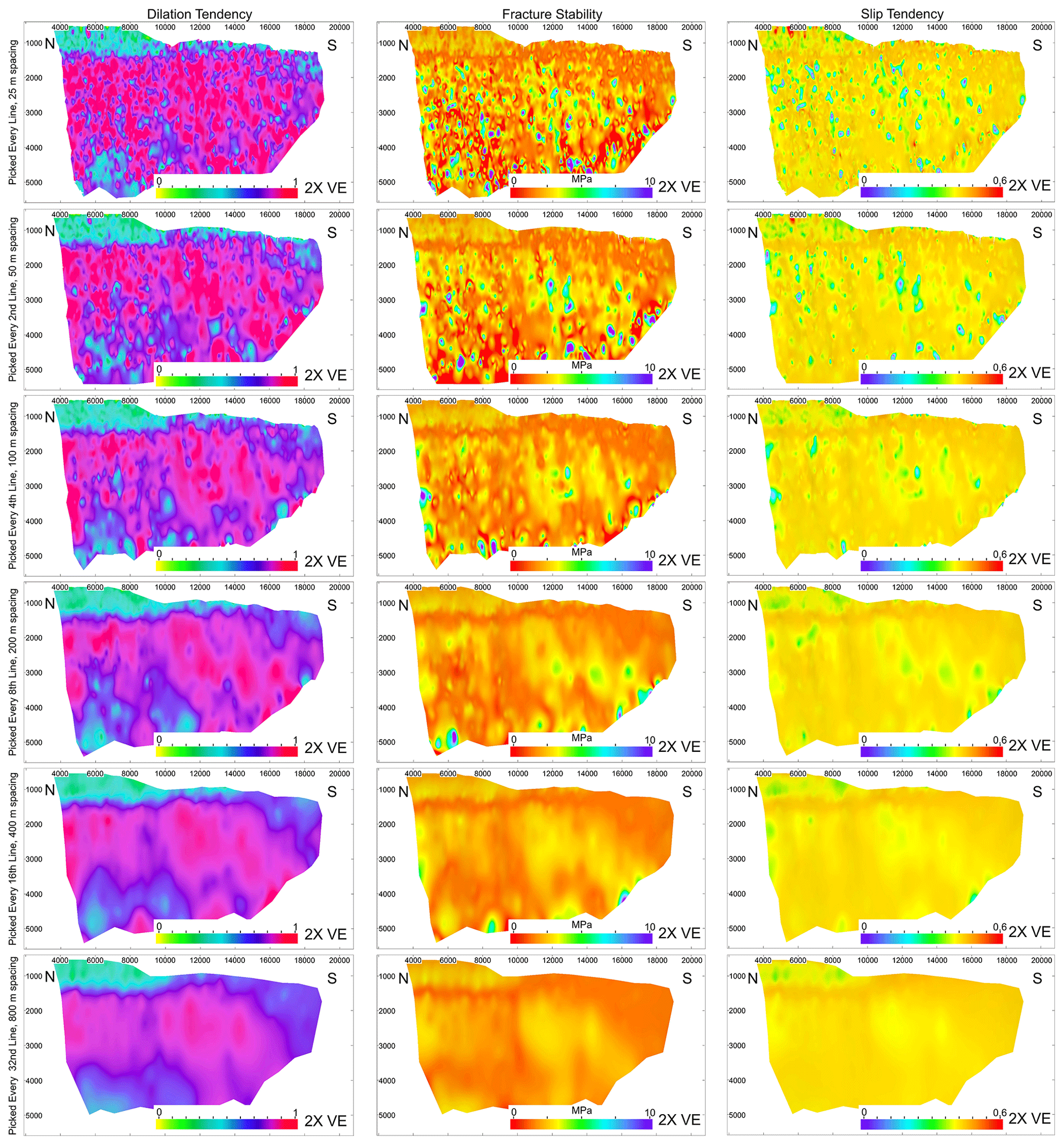
Figure 13Fault plane diagrams showing the fault reactivation potential, specifically dilation tendency, fracture stability and slip tendency for each picking strategy: 25, 50, 100, 200, 400 and 800 m line spacing. Different conclusions regarding fault stability occur due to differing picking strategies. Overall, the stability of the fault is observed to increase with increasing picking strategies. Note that unconstrained triangulation is used for fault surface generation.
Picking strategy influences the overall interpretation of dilation tendency, fracture stability and slip tendency, and all three stability algorithms vary with picking strategy (Fig. 13). Note that the pore pressure values predicted for fracture stability are simply used as an indication for which areas on the fault are more/less stable, rather than to be taken as accurate pressure values that will cause the fault to reactivate. Fault stability varies along fault strike and down fault dip, associated with varying dip attribute values (as previously described in Sect. 4.3.1). At the top of the fault, dip is low such that the fault stability is interpreted to be high. With increasing line spacing, the fault is interpreted to become more stable as patches of steeper dip are removed. At deeper levels on the fault, patches of more and less stable fault are removed with a coarser picking strategy. This creates a fault surface where the overall stability is increased with picking strategy, as the range of predicted dilation tendency and slip tendency values are reduced to lower average values and a higher overall pore pressure would be required to cause the fault to fail (Figs. 12, 13). We can observe that when every line is used for picking (25 m spacing), a large portion of the fault is in failure (i.e. the dilation tendency is over 1; Fig. 14). However, the dilation tendency is reduced as the line spacing is increased. The smoothing of the fault when picked at a 800 m line spacing is reflected in the narrower range in predicted dilation tendency values (Fig. 14). A similar finding has also been recorded by Tao and Alves (2019), where the stability of the fault increases when using coarser picking strategies.
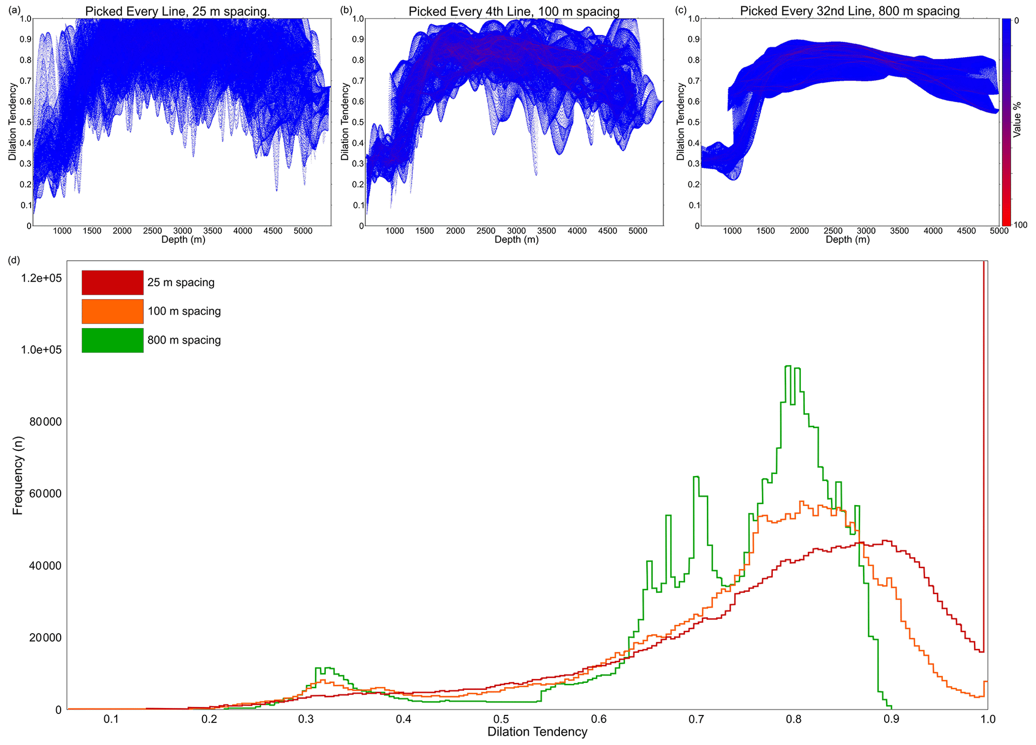
Figure 14(a–c) Plots showing dilation tendency with depth, for scenarios with a line spacing of 25 m (a), 100 m (b) and 800 m (c). Colour intensity reflects the frequency of those values, where blue is 1 % and red is 100 % frequency. (d) Histogram showing frequency of dilation tendency for scenarios picked with a line spacing of 25 m (red), 100 m (orange) and 800 m (green). Note that when every line is picked, a large portion of the values are above 1 (i.e. in failure). Dilation tendency values and their range decrease as the spacing decreases.
Several studies have outlined how fault interpretation is conducted in the subsurface using 2-D and 3-D seismic, specifically fault picking, surface creation and fault cutoff picking (e.g. Badley, 1985; Boult and Freeman, 2007; Krantz and Neely, 2016; Yielding and Freeman, 2016). This methodology is crucial for several fault analyses, specifically, fault growth, fault seal and geomechanical analyses. However, a key step in the methodology appears to be omitted: how does the data sampling strategy, i.e. the spacing of lines for interpretation, affect these analyses? Up until recently, no papers have documented any optimum sampling strategies for fault interpretation in order to make sure all fault details have been captured at an ideal resolution (Tao and Alves, 2019). Tao and Alves (2019) documented an optimum sampling interval fault length ratio (δ) parameter, where the longer the fault, the shorter the sampling distance required. A δ value of 0.03 is suggested for faults that are over 3.5 km in length (as in this example), i.e. measurements at <3 % of the fault length are the minimum required to assess fault segmentation in a reliable way. If the extents of GN1101 only are used (with an approximate fault length of 14 km), noting that the fault is in fact much larger than the extents of this survey, then a sampling interval of a minimum of 420 m would be required. This sampling interval would in fact be much higher if the entire length of the fault is used (approximately 50 km), advocating for up to 1500 m spacing. However, neither of the suggested line spacings would be sufficient to capture all details within this study, as shown by the overly smoothed fault surface and T-D plots when picked at either 400 m or 800 m, which do not capture any of the inherent irregularity or segmentation that occur along the fault.
We show how different results, and hence interpretation, of fault growth, fault stability and fault seal can occur through different picking strategies. Picking faults at increased spacing smooths the fault surface, potentially leading to areas of missed relict breached relays, as well as areas along the fault that might be more prone to up-fault fluid flow through fault reactivation. On the contrary, when fault segments are picked using every crossing line, a combination of human error and/or triangulation method leads to an irregular fault surface with bulls-eye areas of differing fault attribute values. This therefore leads to potential interpretation inaccuracies when fault stability analysis is performed. Suggesting an accurate picking strategy is therefore a balance between smoothing the fault surface to remove irregularities caused by human error and incorporating geological irregularities, for the most accurate fault analyses to be performed in the shortest amount of time invested. It is also important to consider further smoothing caused by seismic resolution, since seismic data cannot capture all irregularities within a fault zone such as jogs and asperities. Hence, an optimum line spacing will also hinge on the limit of seismic resolution. Smoothing is also ingrained in the chosen triangulation method for fault surface creation (Fig. 1).
Faults observed in the field are often recorded as being highly irregular, particularly in mechanically heterogeneous successions, with asperities observed along strike and down dip (e.g. Peacock and Xing, 1994; Childs et al., 1997). However, the inherent imprecise nature of human picking from one line to the next often creates severely uneven fault surfaces, despite rigorous QC (Fig. 15). We can see that the most irregular surface is created when every line is picked. The smoothing increases as spacing increases. Hence, we suggest a line spacing for fault segment picking of 100 m (every fourth line in this example) to most accurately capture fault surface detail for all fault analyses but smooth any severe irregularities between interpreted segments. Three factors are guiding this recommendation: time invested vs. details captured and avoiding noise (irregularity) from individual fault segments (Fig. 15). In terms of an optimum sampling interval fault length ratio (δ) parameter, the suggested 100 m line spacing correlates to a δ value of 0.007 if only the extents of the GN1101 survey are used (Table 2). Note, however, that this suggested line spacing is specific to this case study and is likely to be different for varying sized faults, different tectonic regimes, fault complexity and seismic resolution, as well as potentially varying due to human error and level of QC. Moreover, it could be argued that a best-fit model might prove to be adequate for analysis such as fault stability; hence, using every inline is not suggested as the optimum strategy for such analysis. Specifically, an over irregular fault may lead to the assumption that only bulls-eye areas of the fault may be reactivated; however, any reactivation is likely to influence portions of the fault between each of these bulls-eye patches. However, the degree of best fit is key to this type of analysis. Further, the suggested line spacing is for inlines only that are roughly perpendicular to fault strike. The use of interpreted crosslines may add further irregularity where the faults are oriented parallel to the crossline orientation, due to high ambiguity of the precise fault location, causing any interpretation made on crosslines to rarely tie precisely with the interpretation made on the intersecting inline (as is the case for this study). However, in other cases, the use of crosslines as well as inlines may prove useful. In particular, cases such as faults that are oblique to survey orientation, surveys with wide line spacing or those with poor seismic resolution may benefit from interpretation on crosslines. Hence, continued analysis is required to assess picking strategy using both inlines and crosslines for minor faults that are oblique to the survey orientation.
Table 2Suggested optimum picking strategies, depending on analysis required, and their equivalent sampling interval fault length ratio (δ) based on the extents of the GN1101 survey.
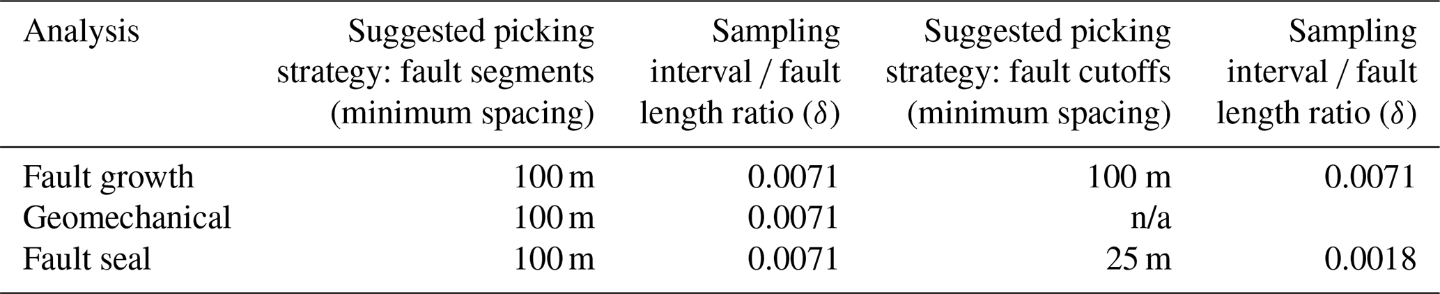
n/a indicates not applicable.
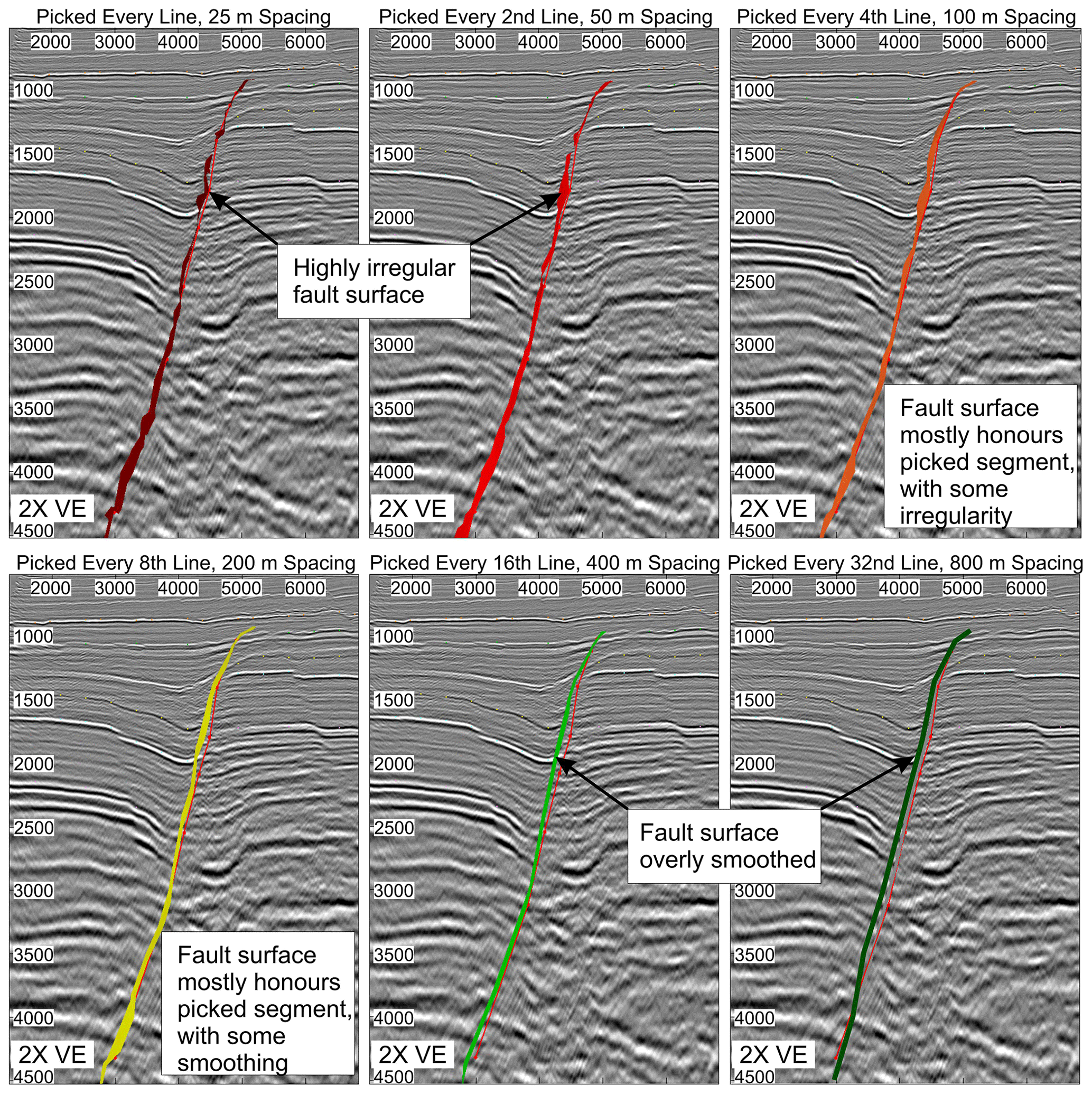
Figure 15Differences in fault surface generation depending on picking strategy: 25, 50, 100, 200, 400 or 800 m line spacing. Picked fault segment is shown as a red line. Note the smoothing that occurs at greater line spacing and the irregularity at narrower line spacing.
A different optimum line spacing is suggested when modelling fault cutoffs. Smoothing is also exaggerated when fault cutoff picking is performed using wide line spacing, regardless of using the same seismic slicing techniques. Picked fault cutoffs using wide line spacing miss important areas, such as drag, for both displacement analysis but also potentially for fault seal analysis. Since all areas of fault segmentation are identified using 100 m line spacing that are also observed using 25 m line spacing, this is the optimum line spacing suggested for fault cutoff modelling when assessing fault growth, in order to reduce time invested but retain the level of detail needed for this analysis (Table 2). However, any areas where drag is not identified through the chosen picking strategy could alter the juxtaposition and hence may lead to incorrect interpretation of the sealing potential of faults. Despite little difference in predicted SGR between 25 and 800 m picking spacing, details incorporating drag into fault seal analysis (that are missed with coarser spacing) are required. In order to ensure all geological irregularities are captured, the finest seismic resolution line spacing is suggested to be used for fault cutoff modelling used for fault seal analysis, specifically 25 m line spacing in this example (δ of 0.0018) (Table 2).
In order to address any uncertainty created by human error, we show how fault picking varies from one person to the next by using the same fault (the VFZ) picked at a 50 m line spacing by two separate interpreters with similar background experience (Fig. 16). The example shown here uses geomechanical analysis (dilation tendency) only, without the added complexity of fault cutoff picking. The overall location of fault segments is approximately the same, with the exception of the vertical extents varying slightly. Further, on some lines, the fault picking is almost identical between the two interpreters (Fig. 16e, f). However, subtle variations in picking techniques are observed. For example, where ambiguity exists due to poor seismic resolution at the fault, combined with a wide fault zone composed of multiple slip surfaces (Fig. 16c), uncertainty ensues when interpreting the precise location of the fault surface. In this example, interpreter one has chosen to pick the hanging wall side of the fault, whereas interpreter two has chosen to pick the fault further into the footwall of the entire fault zone (Fig. 16d). This has also been documented in Faleide et al. (2021), where several interpreters chose different locations to pick the fault: on the footwall, on hanging wall side or within the middle of the fault zone. Variations in the location of fault picks at depth are also observed, caused by poorer seismic resolution at depth, increasing uncertainty when picking the precise fault location. It is these subtle variations in fault segment picking that can cause important variations in the resulting fault attributes. For example, when we examine the dilation tendency on the triangulated fault surfaces, we can see distinct differences that lead to overall changes in fault stability interpretation. Picking the fault segment on the hanging wall side by interpreter one has created a fault surface that is closer to failure than interpreter two's choice, due to resulting variations in fault dip. Due to the vertical extents varying, interpreter two has a more stable area towards the top of the whole fault, whereas only the northernmost area on interpreter one's fault is more stable towards the top of the fault. Overall, interpreter one has generated a fault surface that is less stable than that of interpreter two. Although knowing the precise location of the fault in the subsurface is impossible, it is important to understand how, and to what extent, these slight discrepancies may influence the fault analysis and hence the feasibility of a CO2 storage site. Such uncertainty when interpreting structures within the subsurface have previously been documented (Bond, 2015), which can be attributed to seismic quality (Alcalde et al., 2017) or with cognitive bias, whereby conceptual models of the subsurface can be created through individual training (Bond et al., 2007; Alcalde et al., 2019; Shipton et al., 2020). Although the experience of the interpreters is similar, both factors are likely to play a role within this case study due to the reduced seismic quality at the fault combined with slightly varying professional training.
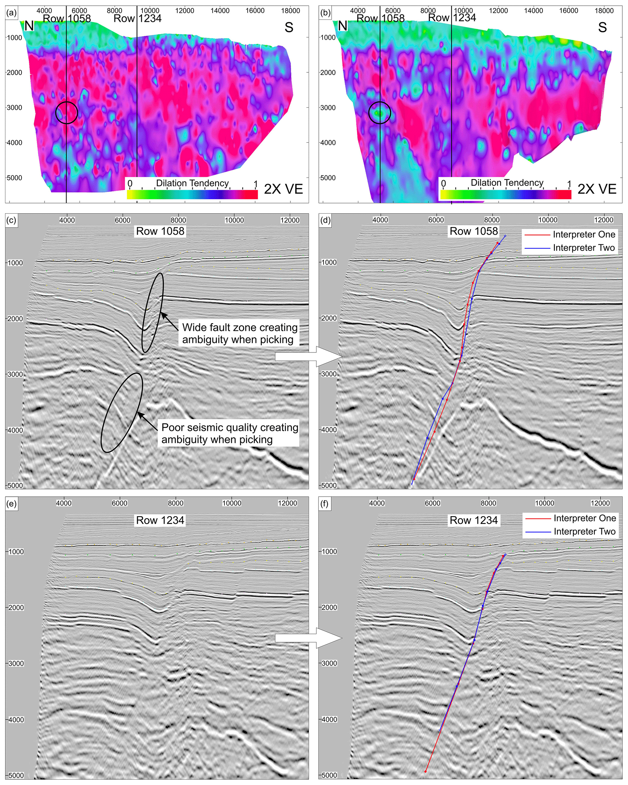
Figure 16Differences in fault picking caused by human error. Two different interpreters have picked the same fault using a line spacing of 50 m. (a, b) Fault plane diagrams show dilation tendency to compare the differences in the fault surface. (a) Interpreter one. (b) Interpreter two. Note that unconstrained triangulation is used for fault surface generation. One area of significant difference is highlighted in the black circle. Vertical lines show locations of intersecting rows 1058 (c, d) and 1234 (e, f). (c) Uninterpreted row 1058 showing a complex portion of the fault zone, leading to ambiguous interpreting. (d) Interpretation of row 1058 by two different interpreters; red: interpreter one, blue: interpreter two. (e) Uninterpreted row 1234 showing a relatively simple portion of the fault zone, leading to similar interpretation from different interpreters. (f) Interpretation of row 1234 by two different interpreters; red: interpreter one, blue: interpreter two.
To assess the effects of triangulation method on fault analysis, we have shown how the fault dip attribute varies with different triangulation methods (Fig. 17). In this example, we have used fault segments picked at every line to examine different triangulation methods. We can see that the dip varies substantially between each triangulation method, particularly when equant triangles that are larger in size (i.e. 400 m) are used. Using larger triangles essentially smooths any irregularities. Conversely, areas of irregularities are increased when equant triangles of a smaller size are used (i.e. 25 m, matching the line spacing). A highly irregular fault surface is produced when a constrained triangulation method is used, as the surface conforms to each data point and lines between adjacent points, rather than creating a “best-fit” surface by gridding through the data points. Unconstrained triangulation also creates an irregular surface but to a lesser degree than constrained triangulation and to a greater extent than gridding. It is important to consider how the triangulation method influences fault attributes, since each triangulation method creates different surfaces. Hence, not only will fault stability analysis vary with picking strategy, but it will also vary with triangulation method chosen. Ultimately, users need to carefully choose the extent to which their data points will be honoured or to create a best-fit surface and acknowledge what this may mean for further analysis. Further, any additional smoothing (as is common in several software packages) will miss any picked irregularity and may lead to incorrect analyses. Caution is therefore required when creating fault surfaces, particularly where automatic smoothing is applied.
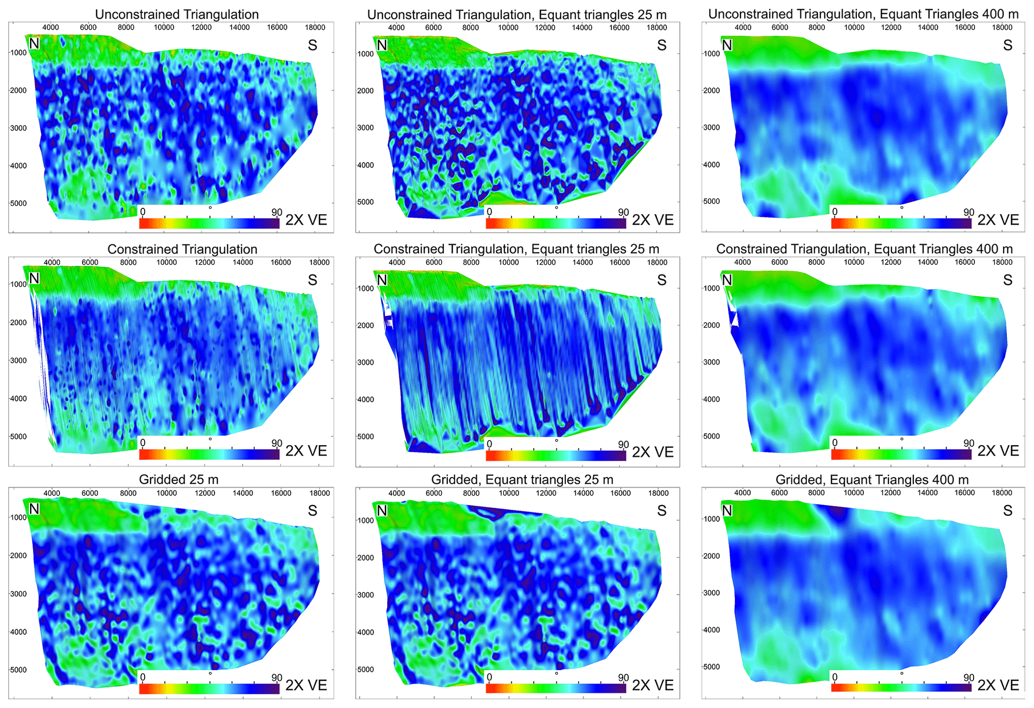
Figure 17Fault plane diagrams created using different triangulation methods for the picking strategy where every line has been interpreted, showing dip attribute. Unconstrained, constrained and gridded triangulation methods have been used, with irregular triangles and equant triangles of different sizes. We can see that vastly different surfaces are created using different techniques, leading to differences in the dip attribute.
As per any interpretation limitations, the seismic quality may vary due to seismic processing, detection limits and resolution, which will impact the resulting fault analyses (Herron, 2011; Alcalde et al., 2017; Faleide et al., 2020). Hence, the suggestions of optimal interpretation techniques described within this paper are likely to not always be applicable to other seismic studies. For example, poorer seismic quality may in fact require closer spaced interpretation. Moreover, these picking strategy suggestions depend on what type of analysis is required and what the overall stratigraphic and structural complexities are. Where increased structural and stratigraphic complexities exist, it is likely that a decreased line spacing is required compared to areas that are less complex.
In addition to the implications of human error, triangulation method and seismic quality, another important consideration when interpreting faults, and what risks and uncertainties are created from the picking strategies, is the time spent picking each fault segment. The amount of time invested in picking each fault segment alters the interpretation and level of irregularity. In a time when tight deadlines are imposed, it is easy to interpret quickly without rigorous QC. This will add another level of uncertainty and inaccuracy to any fault analysis performed. This is shown in Fig. 18, where the interpretation varies depending on the time given to perform the interpretation. Unsurprisingly, more detail is added when extra time is available for interpretation, with fewer mistakes made.
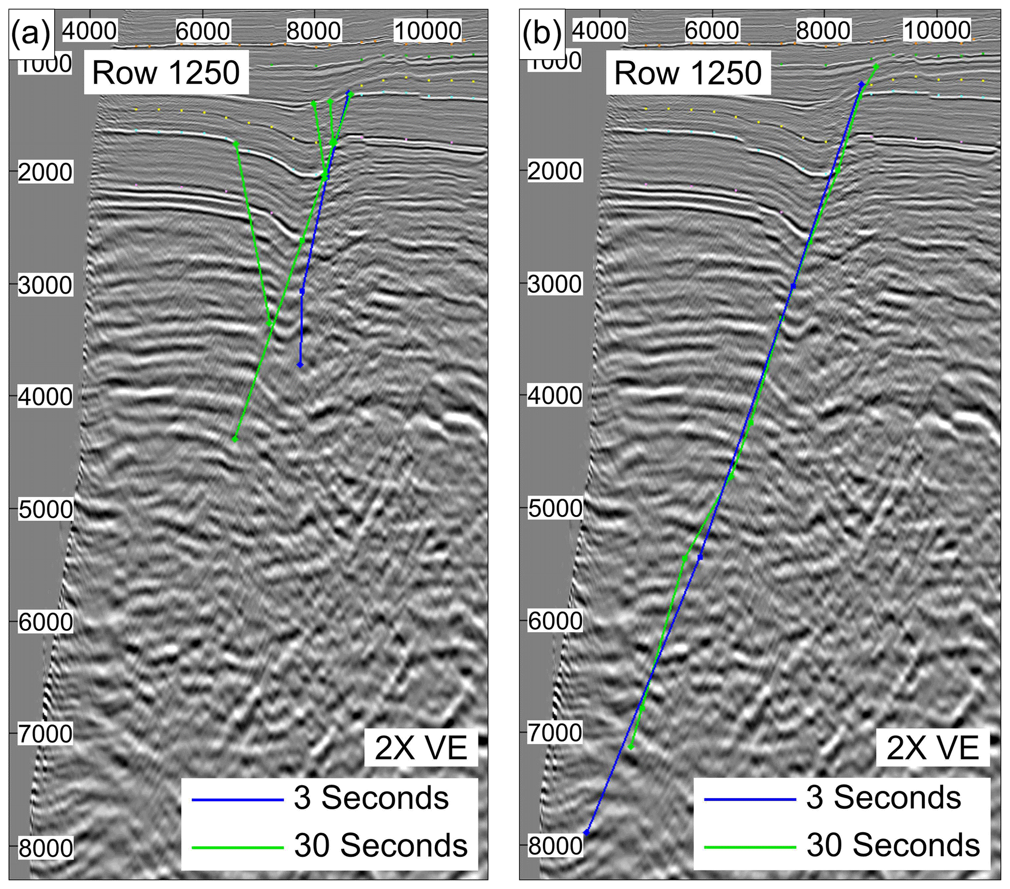
Figure 18Differences in fault picking with different time constraints (3 s vs. 30 s) shown by two separate interpreters (a, b) picked at the same row (row 1250).
Implications of picking strategy on CO2 storage
The predicted shale content of the fault is not shown to vary substantially with picking strategy within this example, when the entire fault is analysed (Fig. 11a, b and c), despite significant differences in the picked fault cutoffs. Whether the fault cutoffs are picked at a spacing of 25 m or 800 m, the SGR calculated remains high. Hence, there is a high fault seal potential, which is likely to retain injected CO2 within the Smeaheia site, regardless of how the fault cutoffs have been picked. However, this could be a product of both the size of the fault, as well as the VShale curve. The high proportion of shale within the sequence means that the shale gouge ratio remains high, regardless of any variations in fault cutoff location. Further, since the throw of the fault reaches up to 1 km, particularly where significant drag is observed (at the northernmost end of the fault), any variations in the size of these drag zones may not influence the juxtaposition sufficiently to alter any fault seal potential. However, some subtle variations in SGR calculated at low VShale overlaps (sand–sand juxtapositions) where the Sognefjord Formation is in the footwall, are recorded with picking strategy (Fig. 11d). Higher SGR calculated using wider picking spacing could be associated with an increased displacement due to the areas of drag either being missed or having a lower amplitude. It is important to note that this is one example of how fault seal potential may vary with picking strategy, and in other examples any differences in calculated SGR may have a more significant impact on the feasibility of a CO2 storage site. For example, areas where drag occurs on small displacement faults, but are missed due to picking strategy, may alter the fault seal potential more significantly in different scenarios. Moreover, different VShale curves, such as those containing a sandier sequence or more substantial differences in VShale values between horizons, may cause significant differences in SGR values with different picking strategy. Hence, no conclusive recommendations for the most accurate picking strategy for fault seal analysis are made using this example. However, picking using every line will capture any and all seismically resolvable variations along the fault. Further, it is important to note that the picking strategy is not the only uncertainty when performing fault seal analysis but may be overshadowed by the significant uncertainty of the gamma-ray transform to a VShale curve and the assumption that the clay content remains constant from the well towards the fault.
Reliable risking of faults for CO2 storage relies on the accuracy of the input parameters. Specifically, this refers to the VShale curve for fault seal analysis (as described above) and accurately capturing the in situ stresses for fault reactivation analysis. More often than not, the picking strategy is overlooked when performing these analyses. However, as we have shown here, the method used for fault picking is crucial for critically analysing the likelihood of fault reactivation upon CO2 injection. The assessment for where a fault is critically stressed or more stable is observed to vary substantially as the picking strategy changes.
Although the likelihood of whether the predicted fault stability for the Smeaheia site is correct, based on accuracy of the input parameters (in situ stress and fault rock cohesion and frictional coefficient), is not fully discussed within this paper, it is important to note that whether the fault may be reactivated upon CO2 injection will be influenced by these factors. For the sake of simplicity, we have used one stress scenario and one fault rock property scenario to assess how fault stability simply varies with picking strategy. However, it is important to note that the fault rock properties chosen for this study are using a previously documented frictional coefficient and cohesion based on estimated clay content in the fault (Meng et al., 2016) rather than measured values. The fault may in fact have higher or lower cohesion and frictional coefficients due to variations in clay content and clay types, along with any cataclasis that is likely to have occurred within the high-porosity sandstone of the Sognefjord Formation. Changing the cohesion and frictional coefficient will alter the predicted pressure that may cause the fault to fail. Hence, the pressure values within this paper are to be used only indicatively for areas that are more or less likely to fail.
We can observe that the predicted SGR values, and hence sealing potential of the fault, are high, reducing the risk for CO2 storage regardless of picking strategy used. Conversely, the likelihood of the fault to reactivate is also high, increasing the risk for CO2 storage. However, the variations to the fault reactivation potential dependent on picking strategy are significant, causing uncertainties for this analysis. When we use our suggested optimum picking strategy of 100 m, we can see patches of the fault where the risk of reactivation is low but which also contain areas where the fault is close to failure (Figs. 12 and 13). Hence, under these limited modelled scenarios, there is a high likelihood for the fault to reactivate upon CO2 injection.
The line spacing chosen to pick both the fault segments and fault cutoffs will influence the analysis performed on the faults, with the results varying with picking strategy. We can observe that using a wider line spacing
-
underestimates fault segmentation;
-
causes inaccurate interpretation of the location of fault segments;
-
predicts a higher SGR and hence higher fault-sealing potential in this example;
-
smooths the fault such that subtle variations in dip and strike are not obvious; and
-
predicts an overall more stable fault in this example.
Through observations regarding fault growth analysis, we show that the optimum picking strategy for this example is using a spacing of 100 m. This picking strategy not only identifies all fault segments that are observed using every line but also smooths the fault such that any irregularities caused by human error and triangulation method are removed but retains detail for accurate geomechanical analysis. While using 100 m line spacing for fault segmentation and fault cutoff picking is suitable for fault growth modelling and geomechanical modelling, a different approach may be required for detailed fault seal analysis. Although the overall SGR is very similar when picked using a spacing of 25 m or 800 m, subtle variations, that may be critical in other examples, are observed. Specifically, a potential overestimation of the SGR occurs when a wider picking strategy is used. Hence, picking fault cutoffs using every line spacing is suggested, as this strategy will capture all geological irregularities important for the fault seal.
The authors do not have permission to share data.
EAHM designed the methodology for the investigation, along with AB. EAHM carried out the investigation, with help from MJM. EAHM prepared the manuscript and figures with scientific input, discussions and proofing from all co-authors. AB provided funding for the research.
The authors declare that they have no known competing financial interest or personal relationships that could have appeared to influence the work reported in this paper.
This is a contribution of the FRISK project, supported by the Research Council of Norway. Support from the NCCS Centre is acknowledged, performed under the Norwegian research programme Centres for Environment-friendly Energy Research (FME). The authors acknowledge the following partners for their contributions: Aker Solutions, Ansaldo Energia, CoorsTek Membrane Sciences, EMGS, Equinor, Gassco, Krohne, Larvik Shipping, Lundin, Norcem, Norwegian Oil and Gas, Quad Geometrics, Total, Vår Energi and the Research Council of Norway. Badley Geoscience Ltd. is thanked for their academic license of T7. Warm thanks are given to Peter Bretan and Andrew Foster for their software support. Great thanks are given to reviewers Christopher Jackson and Rūta Karolytė for their detailed and constructive comments, which significantly improved the quality of this contribution.
This research has been supported by the Norges Forskningsråd (grant nos. 295061 and 257579/E20).
This paper was edited by David Healy and reviewed by Ruta Karolyte and Christopher Jackson.
Alcalde, J., Bond, C. E., Johnson, G., Ellis, J. F., and Butler, R. W.: Impact of seismic image quality on fault interpretation uncertainty, GSA Today, 27, 4–10, https://doi.org/10.1130/GSATG282A.1, 2017.
Alcalde, J., Bond, C. E., Johnson, G., Kloppenburg, A., Ferrer, O., Bell, R., and Ayarza, P.: Fault interpretation in seismic reflection data: an experiment analysing the impact of conceptual model anchoring and vertical exaggeration, Solid Earth, 10, 1651–1662, https://doi.org/10.5194/se-10-1651-2019, 2019.
Allan, U. S.: Model for hydrocarbon migration and entrapment within faulted structures, AAPG Bull., 73, 803–811, https://doi.org/10.1306/44B4A271-170A-11D7-8645000102C1865D, 1989.
Andrews, J. S., Fintland, T. G., Helstrup, O. A., Horsrud, P., and Raaen, A. M.: Use of unique database of good quality stress data to investigate theories of fracture initiation, fracture propagation and the stress state in the subsurface, 50th US Rock Mechanics/Geomechanics Symposium, American Rock Mechanics Association, June 2016.
Araya-Polo, M., Dahlke, T., Frogner, C., Zhang, C., Poggio, T., and Hohl, D.: Automated fault detection without seismic processing, The Leading Edge, 36, 208–214, https://doi.org/10.1190/tle36030208.1, 2017.
Avseth, P., Mukerji, T., and Mavko, G.: Quantitative seismic interpretation: Applying rock physics tools to reduce interpretation risk, Cambridge University Press, Cambridge, https://doi.org/10.1017/CBO9780511600074, 2010.
Badley, M. E.: Practical seismic interpretation, Int. Human Res. Dev., Boston, MA, 266 pp., 1985.
Badley, M. E., Price, J. D., Dahl, C. R., and Agdestein, T.: The structural evolution of the northern Viking Graben and its bearing upon extensional modes of basin formation, J. Geol. Soc., 145, 455–472, https://doi.org/10.1144/gsjgs.145.3.0455, 1988.
Barton, C. A., Zoback, M. D., and Moos, D.: Fluid flow along potentially active faults in crystalline rock, Geology, 23, 683–686, https://doi.org/10.1130/0091-7613(1995)023%3C0683:FFAPAF%3E2.3.CO;2, 1995.
Bell, R. E., Jackson, C. A. L., Elliott, G. M., Gawthorpe, R. L., Sharp, I. R., and Michelsen, L.: Insights into the development of major rift-related unconformities from geologically constrained subsidence modelling: Halten Terrace, offshore mid Norway, Basin Res., 26, 203–224, https://doi.org/10.1111/bre.12049, 2014.
Benedicto, A., Schultz, R. A., and Soliva, R.: Layer thickness and the shape of faults, Geophys. Res. Lett., 30, 2076, https://doi.org/10.1029/2003GL018237, 2003.
Bense, V. F. and Van Balen, R.: The effect of fault relay and clay smearing on groundwater flow patterns in the Lower Rhine Embayment, Basin Res., 16, 397–411, https://doi.org/10.1111/j.1365-2117.2004.00238.x, 2004.
Birol, F.: World energy outlook, Paris: International Energy Agency, 23, p. 329, 2008.
Bond, C. E.: Uncertainty in structural interpretation: Lessons to be learnt, J. Struct. Geol., 74, 185–200, https://doi.org/10.1016/j.jsg.2015.03.003, 2015.
Bond, C. E., Gibbs, A. D., Shipton, Z. K., and Jones, S.: What do you think this is? “Conceptual uncertainty” in geoscience interpretation, GSA Today, 17, 4, https://doi.org/10.1130/GSAT01711A.1, 2007.
Boult, P. and Freeman, B.: Using faults as an aid to horizon mapping in areas of poor 2D seismic: Otway Basin example, MESA J., 46, 4–9, 2007.
Bretan, P., Yielding, G., and Jones, H.: Using calibrated shale gouge ratio to estimate hydrocarbon column heights, AAPG Bull., 87, 397–413, https://doi.org/10.1306/08010201128, 2003.
Bretan, P., Yielding, G., Mathiassen, O. M., and Thorsnes, T.: Fault-seal analysis for CO2 storage: an example from the Troll area, Norwegian Continental Shelf, Petrol. Geosci., 17, 181–192, https://doi.org/10.1144/1354-079310-025, 2011.
Brodsky, E. E., Gilchrist, J. J., Sagy, A., and Collettini, C.: Faults smooth gradually as a function of slip, Earth Planet. Sci. Lett., 302, 185–193, https://doi.org/10.1016/j.epsl.2010.12.010, 2011.
Brudy, M. and Kjørholt, H.: Stress orientation on the Norwegian continental shelf derived from borehole failures observed in high-resolution borehole imaging logs, Tectonophysics, 337, 65–84, https://doi.org/10.1016/S0040-1951(00)00299-7, 2001.
Cartwright, J. A., Trudgill, B. D., and Mansfield, C. S.: Fault growth by segment linkage: an explanation for scatter in maximum displacement and trace length data from the Canyonlands Grabens of SE Utah, J. Struct. Geol., 17, 1319–1326, https://doi.org/10.1016/0191-8141(95)00033-A, 1995.
Cartwright, J. A., Mansfield, C., and Trudgill, B.: The growth of normal faults by segment linkage. Geological Society, London, Special Publications, 99, 163–177, https://doi.org/10.1144/GSL.SP.1996.099.01.13, 1996.
Chiaramonte, L., Zoback, M. D., Friedmann, J., and Stamp, V.: Seal integrity and feasibility of CO2 sequestration in the Teapot Dome EOR pilot: geomechanical site characterization, Environ. Geol., 54, 1667–1675, https://doi.org/10.1007/s00254-007-0948-7, 2008.
Childs, C., Watterson, J., and Walsh, J. J.: Fault overlap zones within developing normal fault systems, J. Geol. Soc., 152, 535–549, https://doi.org/10.1144/gsjgs.152.3.0535, 1995.
Childs, C., Walsh, J. J., and Watterson, J.: Complexity in fault zone structure and implications for fault seal prediction, in: Norwegian Petroleum Society Special Publications, 7, 61–72, https://doi.org/10.1016/S0928-8937(97)80007-0, 1997.
Childs, C., Holdsworth, R. E., Jackson, C. A. L., Manzocchi, T., Walsh, J. J., and Yielding, G.: Introduction to the geometry and growth of normal faults, Geological Society, London, Special Publications, 439, 1–9. https://doi.org/10.1144/SP439.24, 2017.
Chiquet, P., Daridon, J. L., Broseta, D., and Thibeau, S.: CO2/water interfacial tensions under pressure and temperature conditions of CO2 geological storage, Energ. Convers. Manage., 48, 736–744, https://doi.org/10.1016/j.enconman.2006.09.011, 2007.
Cowie, P. A.: A healing–reloading feedback control on the growth rate of seismogenic faults, J. Struct. Geol., 20, 1075–1087, https://doi.org/10.1016/S0191-8141(98)00034-0, 1998.
Cowie, P. A. and Scholz, C. H.: Displacement-length scaling relationship for faults: data synthesis and discussion, J. Struct. Geol., 14, 1149–1156, https://doi.org/10.1016/0191-8141(92)90066-6, 1992a.
Cowie, P. A. and Scholz, C. H.: Physical explanation for displacement-length relationship of faults using a post-yield fracture mechanics model, J. Struct. Geol., 14, 1133–1133, https://doi.org/10.1016/0191-8141(92)90065-5, 1992b.
Daniel, R. F. and Kaldi, J. G.: Evaluating seal capacity of caprocks and intraformational barriers for the geosequestration of CO2, PESA Eastern Australian Basins Symposium III, Sydney, Australia, September 2008.
Dawers, N. H. and Anders, M. H.: Displacement-length scaling and fault linkage, J. Struct. Geol., 17, 607–614, https://doi.org/10.1016/0191-8141(94)00091-D, 1995.
Deng, C., Fossen, H., Gawthorpe, R. L., Rotevatn, A., Jackson, C. A. L., and FazliKhani, H.: Influence of fault reactivation during multiphase rifting: The Oseberg area, northern North Sea rift, Mar. Petrol. Geol., 86, 1252–1272, https://doi.org/10.1016/j.marpetgeo.2017.07.025, 2017.
Dreyer, T., Whitaker, M., Dexter, J., Flesche, H., and Larsen, E.: From spit system to tide-dominated delta: integrated reservoir model of the Upper Jurassic Sognefjord Formation on the Troll West Field, in: Geological Society, London, Petroleum Geology Conference series, 6, 423–448, Geological Society of London, https://doi.org/10.1144/0060423, 2005.
Duffy, O. B., Bell, R. E., Jackson, C. A. L., Gawthorpe, R. L., and Whipp, P. S.: Fault growth and interactions in a multiphase rift fault network: Horda Platform, Norwegian North Sea, J. Struct. Geol., 80, 99–119, https://doi.org/10.1016/j.jsg.2015.08.015, 2015.
EU Commission: Communication from the commission to the European parliament, the European Council, the Council, the European economic and social committee, the committee of the regions and the European investment bank, in: A Clean Planet for All. A European Strategic Long-Term Vision for a Prosperous, Modern, Competitive and Climate Neutral Economy, Publication Office of the European Union, Brussels, 2018.
Faleide, T. S., Braathen, A., Lecomte, I., Mulrooney, M. J., Anell, I., Midtkandal, I., and Planke, S.: Testing Seismic Interpretations of Faults by Modelling; Viable Geometries versus Seismic Resolution in the Subsurface, 82nd EAGE Annual Conference & Exhibition 1, 1–5, https://doi.org/10.3997/2214-4609.202011930, 2020.
Faleide, T. S., Braathen, A., Lecomte, I., Mulrooney, M. J., Midtkandal, I., Bugge, A. J., and Planke, S.: Impacts of seismic resolution on fault interpretations: Insights from seismic modelling, Tectonophysics, in review, 2021.
Færseth, R. B.: Interaction of Permo-Triassic and Jurassic extensional fault-blocks during the development of the northern North Sea, J. Geol. Soc., 153, 931–944, https://doi.org/10.1144/gsjgs.153.6.0931, 1996.
Færseth, R. B.: Shale smear along large faults: continuity of smear and the fault seal capacity, J. Geol. Soc., 163, 741–751, https://doi.org/10.1144/0016-76492005-162, 2006.
Færseth, R. B., Gabrielsen, R. H., and Hurich, C. A.: Influence of basement in structuring of the North Sea basin, offshore southwest Norway, Norsk Geologisk Tidsskrift, 75, 105–119, 1995.
Ferrill, D. A., Winterle, J., Wittmeyer, G., Sims, D., Colton, S., Armstrong, A., and Morris, A. P.: Stressed rock strains groundwater at Yucca Mountain, Nevada, GSA Today, 9, 1–8, 1999a.
Ferrill, D. A., Stamatakos, J. A., and Sims, D.: Normal fault corrugation: Implications for growth and seismicity of active normal faults, J. Struct. Geol., 21, 1027–1038, https://doi.org/10.1016/S0191-8141(99)00017-6, 1999b.
Fisher, Q. J. and Knipe, R.: Fault sealing processes in siliciclastic sediments, Geological Society, London, Special Publications, 147, 117–134, https://doi.org/10.1144/GSL.SP.1998.147.01.08, 1998.
Foxford, K. A., Walsh, J. J., Watterson, J., Garden, I. R., Guscott, S. C., and Burley, S. D.: Structure and content of the Moab Fault Zone, Utah, USA, and its implications for fault seal prediction, Geological Society, London, Special Publications, 147, 87–103, https://doi.org/10.1144/GSL.SP.1998.147.01.06, 1998.
Fristad, T., Groth, A., Yielding, G., and Freeman, B.: Quantitative fault seal prediction: a case study from Oseberg Syd, in: Norwegian Petroleum Society Special Publications, 7, 107–124, https://doi.org/10.1016/S0928-8937(97)80010-0, 1997.
Fulljames, J. R., Zijerveld, L. J. J., and Franssen, R. C. M. W.: Fault seal processes: systematic analysis of fault seals over geological and production time scales, in: Norwegian Petroleum Society Special Publications, 7, 51–59, https://doi.org/10.1016/S0928-8937(97)80006-9, 1997.
Goldsmith, P. J.: Exploration potential east of the Troll Field, offshore Norway, after dry well 32/4-1, in: Norwegian Petroleum Society Special Publications, 9, 65–97, https://doi.org/10.1016/S0928-8937(00)80010-7, 2000.
Gradstein, F. M. and Waters, C. N.: Stratigraphic Guide to the Cromer Knoll, Shetland and Chalk Groups, North Sea and Norwegian Sea, Newsl. Stratigr., 49, 71–280, https://doi.org/10.1127/nos/2016/0071, 2016.
Halland, E. K., Johansen, W. T., and Riis, F.: CO2 Storage Atlas: Norwegian North Sea, Norwegian Petroleum Directorate, PO Box 600, NO–4003 Stavanger, Norway, available at: http://www.npd.no/no/Publikasjoner/Rapporter/CO2-lagringsatlas (last access: July 2020), 2011.
Herron, D. A.: First steps in seismic interpretation, Society of Exploration Geophysicists, 203 pp., https://doi.org/10.1190/1.9781560802938, 2011.
Hillis, R. R. and Nelson, E. J. In situ stresses in the North Sea and their applications: Petroleum geomechanics from exploration to development, in: Geological Society, London, Petroleum Geology Conference series (Vol. 6, No. 1, pp. 551–564), Geological Society of London, https://doi.org/10.1144/0060551, 2005.
Holgate, N. E., Jackson, C. A. L., Hampson, G. J., and Dreyer, T.: Sedimentology and sequence stratigraphy of the middle–upper jurassic krossfjord and fensfjord formations, Troll Field, northern North Sea, Petrol. Geosci., 19, 237–258, https://doi.org/10.1144/petgeo2012-039, 2013.
Huggins, P., Watterson, J., Walsh, J. J., and Childs, C.: Relay zone geometry and displacement transfer between normal faults recorded in coal-mine plans, J. Struct. Geol., 17, 1741–1755, https://doi.org/10.1016/0191-8141(95)00071-K, 1995.
Intergovernmental Panel on Climate Change: Climate Change 2014: Synthesis Report, Contribution of Working Groups I, II and III to the Fifth Assessment Report of the Intergovernmental Panel on Climate Change, edited by: Core Writing Team, Pachauri, R. K. and Meyer, L. A., IPCC, Geneva, Switzerland, 151 pp., 2014.
Intergovernmental Panel on Climate Change: Summary for Policymakers, in: Global Warming of 1.5 ∘C. An IPCC Special Report on the impacts of global warming of 1.5 ∘C above pre-industrial levels and related global greenhouse gas emission pathways, in the context of strengthening the global response to the threat of climate change, sustainable development, and efforts to eradicate poverty, edited by: Masson-Delmotte, V., Zhai, P., Pörtner, H.-O., Roberts, D., Skea, J., Shukla, P. R., Pirani, A., Moufouma-Okia, W., Péan, C., Pidcock, R., Connors, S., Matthews, J. B. R., Chen, Y., Zhou, X., Gomis, M. I., Lonnoy, E., Maycock, T., Tignor, M., and Waterfield, T., World Meteorological Organization, Geneva, Switzerland, 32 pp., 2018.
Isaksen, G. H. and Ledje, K. H. I.: Source rock quality and hydrocarbon migration pathways within the greater Utsira High area, Viking Graben, Norwegian North Sea, AAPG Bull., 85, 861–883, https://doi.org/10.1306/8626CA23-173B-11D7-8645000102C1865D, 2001.
Jackson, C. A. L. and Rotevatn, A.: 3D seismic analysis of the structure and evolution of a salt-influenced normal fault zone: a test of competing fault growth models, J. Struct. Geol., 54, 215–234, https://doi.org/10.1016/j.jsg.2013.06.012, 2013.
Jackson, C. A. L., Bell, R. E., Rotevatn, A., and Tvedt, A. B.: Techniques to determine the kinematics of synsedimentary normal faults and implications for fault growth models, Geological Society, London, Special Publications, 439, 187–217, https://doi.org/10.1144/SP439.22, 2017a.
Jackson, C. A. L., Rotevatn, A., Tvedt, A., and Bell, R. E.: The role of gravitational collapse in controlling the evolution of crestal fault systems (Espirito Santo Basin, SE Brazil)-Discussion, J. Struct. Geol., 98, 95–97, https://doi.org/10.1016/j.jsg.2016.09.011, 2017b.
Jennings, J. B.: Capillary pressure techniques: application to exploration and development geology, AAPG Bull., 71, 1196–1209, https://doi.org/10.1306/703C8047-1707-11D7-8645000102C1865D, 1987.
Justwan, H. and Dahl, B.: Quantitative hydrocarbon potential mapping and organofacies study in the Greater Balder Area, Norwegian North Sea, in: Geological Society, London, Petroleum Geology Conference series, 6, 1317–1329, Geological Society of London, https://doi.org/10.1144/0061317, 2005.
Karolytė, R., Johnson, G., Yielding, G., and Gilfillan, S. M.: Fault seal modelling–the influence of fluid properties on fault sealing capacity in hydrocarbon and CO2 systems, Petrol. Geosci., 26, 481–497, https://doi.org/10.1144/petgeo2019-126, 2020.
Kim, Y. S. and Sanderson, D. J.: The relationship between displacement and length of faults: a review, Earth-Sci. Rev., 68, 317–334, https://doi.org/10.1016/j.earscirev.2004.06.003, 2005.
Knipe, R. J.: Faulting processes and fault seal, in: Structural and tectonic modelling and its application to petroleum geology, Norwegian Petroleum Society Special Publications, 1, 325–342, https://doi.org/10.1016/B978-0-444-88607-1.50027-9, 1992.
Knipe, R. J., Fisher, Q. J., Jones, G., Clennell, M. R., Farmer, A. B., Harrison, A., Kidd, B., McAllister, E. R. P. J., Porter, J. R., and White, E. A.: Fault seal analysis: successful methodologies, application and future directions, in: Norwegian Petroleum Society Special Publications, 7, 15–38, https://doi.org/10.1016/S0928-8937(97)80004-5, 1997.
Krantz, B. and Neely, T.: Subsurface structural interpretation: The significance of 3-D structural frameworks, edited by: Krantz, B., Ormand, C., and Freeman, B., 3-D structural interpretation: Earth, mind, and machine: AAPG Memoir, 111, 155–171, https://doi.org/10.1306/13561988M1113181, 2016.
Kyrkjebø, R., Gabrielsen, R. H., and Faleide, J. I.: Unconformities related to the Jurassic–Cretaceous synrift–post-rift transition of the northern North Sea, J. Geol. Soc., 161, 1–17, https://doi.org/10.1144/0016-764903-051, 2004.
Lauritsen, H., Kassold, S., Meneguolo, R., and Furre, A.: Assessing potential influence of nearby hydrocarbon production on CO2 storage at Smeaheia, in: Fifth CO2 Geological Storage Workshop, 2018, 1–5, European Association of Geoscientists & Engineers, https://doi.org/10.3997/2214-4609.201802970, 2018.
Lindsay, N. G., Murphy, F. C., and Walsh, J. J.: Watterson. Outcrop studies of shale smears on fault surfaces, The geological modelling of hydrocarbon reservoirs and outcrop analogues, edited by: Flint, S. S. and Bryant, I. D., International Association of Sedimentology, Special Publications, 15, 113–123, https://doi.org/10.1002/9781444303957.ch6, 1993.
Lothe, A. E., Bergmo, P. E., and Grimstad, A. A.: Storage Resources for Future European CCS Deployment; A Roadmap for a Horda CO2 Storage Hub, Offshore Norway, in: Proceedings of the 10th Trondheim Conference on CO2 Capture, Transport and Storage (TCCS-10), 17–19 June 2019.
Lyon, P. J., Boult, P. J., Hillis, R. R., and Mildren, S. D.: Sealing by shale gouge and subsequent seal breach by reactivation: A case study of the Zema Prospect, Otway Basin, edited by: Boult, P. and Kaldi, J., Evaluating Fault and Cap Rock Seals, AAPG Hedberg Series, AAPG, Tulsa, OK (2005), no. 2, pp. 179–197, 2005.
Manzocchi, T., Childs, C., and Walsh, J. J.: Faults and fault properties in hydrocarbon flow models, Geofluids, 10, 94–113, https://doi.org/10.1111/j.1468-8123.2010.00283.x, 2010.
Meng, L., Fu, X., Lv, Y., Li, X., Cheng, Y., Li, T., and Jin, Y.: Risking fault reactivation induced by gas injection into depleted reservoirs based on the heterogeneity of geomechanical properties of fault zones, Petrol. Geosci., 23, 29–38, https://doi.org/10.1144/petgeo2016-031, 2016.
Mildren, S. D., Hillis, R. R., Lyon, P. J., Meyer, J. J., Dewhurst, D. N., and Boult, P. J.: FAST: a new technique for geomechanical assessment of the risk of reactivation-related breach of fault seals, edited by: Boult, P. and Kaldi, J., Evaluating Fault and Cap Rock Seals, AAPG Hedberg Series, AAPG, Tulsa, OK (2005), no. 2, pp. 73–85, 2005.
Miocic, J. M., Johnson, G., and Bond, C. E.: Uncertainty in fault seal parameters: implications for CO2 column height retention and storage capacity in geological CO2 storage projects, Solid Earth, 10, 951–967, https://doi.org/10.5194/se-10-951-2019, 2019.
Mondol, N. H., Fawad, M., and Park, J.: Petrophysical Analysis And Rock Physics Diagnostics Of Sognefjord Formation In The Smeaheia Area, Northern North Sea, in: Fifth CO2 Geological Storage Workshop, 2018, 1–5, European Association of Geoscientists & Engineers, https://doi.org/10.3997/2214-4609.201802951, 2018.
Morley, C. K.: Patterns of displacement along large normal faults: implications for basin evolution and fault propagation, based on examples from East Africa, AAPG Bulletin, 83, 613–634, https://doi.org/10.1306/00AA9C0A-1730-11D7-8645000102C1865D, 1999.
Morley, C. K., Nelson, R. A., Patton, T. L., and Munn, S. G.: Transfer zones in the East African rift system and their relevance to hydrocarbon exploration in rifts, AAPG Bull., 74, 1234–1253, https://doi.org/10.1306/0C9B2475-1710-11D7-8645000102C1865D, 1990.
Morris, A., Ferrill, D. A., and Henderson, D. B.: Slip-tendency analysis and fault reactivation, Geology, 24, 275–278, https://doi.org/10.1130/0091-7613(1996)024%3C0275:STAAFR%3E2.3.CO;2, 1996.
Mulrooney, M. J., Osmond, J. L., Skurtveit, E., Faleide, J. I., and Braathen, A.: Structural analysis of the Smeaheia fault block, a potential CO2 storage site, northern Horda Platform, North Sea, Mar. Petrol. Geol., 121, 104598, https://doi.org/10.1016/j.marpetgeo.2020.104598, 2020.
Nicol, A., Watterson, J., Walsh, J. J., and Childs, C.: The shapes, major axis orientations and displacement patterns of fault surfaces, J. Struct. Geol., 18, 235–248, https://doi.org/10.1016/S0191-8141(96)80047-2, 1996.
Nicol, A., Walsh, J., Berryman, K., and Nodder, S.: Growth of a normal fault by the accumulation of slip over millions of years, J. Struct. Geol., 27, 327–342, https://doi.org/10.1016/j.jsg.2004.09.002, 2005.
Nicol, A., Walsh, J. J., Villamor, P., Seebeck, H., and Berryman, K. R.: Normal fault interactions, paleoearthquakes and growth in an active rift, J. Struct. Geol., 32, 1101–1113, https://doi.org/10.1016/j.jsg.2010.06.018, 2010.
Nybakken, S. and Bäckstrøm, S. A.: Shetland Group: stratigraphic subdivision and regional correlation in the Norwegian North Sea, in: Correlation in Hydrocarbon Exploration, Springer, Dordrecht, 253–269, https://doi.org/10.1007/978-94-009-1149-9_20, 1989.
Patruno, S., Hampson, G. J., Jackson, C. A. L., and Whipp, P. S.: Quantitative progradation dynamics and stratigraphic architecture of ancient shallow-marine clinoform sets: a new method and its application to the Upper Jurassic Sognefjord Formation, Troll Field, offshore Norway, Basin Res., 27, 412–452, https://doi.org/10.1111/bre.12081, 2015.
Peacock, D. C. P. and Sanderson, D. J.: Displacements, segment linkage and relay ramps in normal fault zones, J. Struct. Geol., 13, 721–733, https://doi.org/10.1016/0191-8141(91)90033-F, 1991.
Peacock, D. C. P. and Sanderson, D. J.: Geometry and development of relay ramps in normal fault systems, AAPG Bull., 78, 147–165, https://doi.org/10.1306/BDFF9046-1718-11D7-8645000102C1865D, 1994.
Peacock, D. C. P. and Xing, Z.: Field examples and numerical modelling of oversteps and bends along normal faults in cross-section, Tectonophysics, 234, 147–167, https://doi.org/10.1016/0040-1951(94)90209-7, 1994.
Rider, M.: The geological interpretation of well logs second edition, Rider–French Consulting Ltd, Sutherland, The United Kingdom, 126–128, 2000.
Ringrose, P. S., Thorsen, R., Zweigel, P., Nazarian, B., Furre, A. K., Paasch, B., Thompson, N., and Karstad, P. I.: Ranking and Risking Alternative CO2 Storage Sites Offshore Norway, in: Fourth Sustainable Earth Sciences Conference, 2017, 1–5, European Association of Geoscientists & Engineers, https://doi.org/10.3997/2214-4609.201702142, 2017.
Rogelj, J., Den Elzen, M., Höhne, N., Fransen, T., Fekete, H., Winkler, H., Schaeffer, R., Sha, F., Riahi, K., and Meinshausen, M.: Paris Agreement climate proposals need a boost to keep warming well below 2 C, Nature, 534, 631–639, https://doi.org/10.1038/nature18307, 2016.
Rotevatn, A., Fossen, H., Hesthammer, J., Aas, T. E., and Howell, J. A.: Are relay ramps conduits for fluid flow? Structural analysis of a relay ramp in Arches National Park, Utah, Geological Society, London, Special Publications, 270, 55–71, https://doi.org/10.1144/GSL.SP.2007.270.01.04, 2007.
Rotevatn, A., Tveranger, J., Howell, J. A., and Fossen, H.: Dynamic investigation of the effect of a relay ramp on simulated fluid flow: geocellular modelling of the Delicate Arch Ramp, Utah, Petrol. Geosci., 15, 45–58, https://doi.org/10.1144/1354-079309-779, 2009.
Rotevatn, A., Kristensen, T. B., Ksienzyk, A. K., Wemmer, K., Henstra, G. A., Midtkandal, I., Grundvåg, S. A., and Andresen, A.: Structural inheritance and rapid rift-length establishment in a multiphase rift: The East Greenland rift system and its Caledonian orogenic ancestry, Tectonics, 37, 1858–1875, https://doi.org/10.1029/2018TC005018, 2018.
Rotevatn, A., Jackson, C. A. L., Tvedt, A. B., Bell, R. E., and Blækkan, I.: How do normal faults grow?, J. Struct. Geol., 125, 174–184, https://doi.org/10.1016/j.jsg.2018.08.005, 2019.
Rutqvist, J., Birkholzer, J., Cappa, F., and Tsang, C. F.: Estimating maximum sustainable injection pressure during geological sequestration of CO2 using coupled fluid flow and geomechanical fault-slip analysis, Energ. Convers. Manage., 48, 1798–1807, https://doi.org/10.1016/j.enconman.2007.01.021, 2007.
Sagy, A., Brodsky, E. E., and Axen, G. J.: Evolution of fault-surface roughness with slip, Geology, 35, 283–286, https://doi.org/10.1130/G23235A.1, 2007.
Schöpfer, M. P., Childs, C., and Walsh, J. J.: Localisation of normal faults in multilayer sequences, J. Struct. Geol., 28, 816–833, https://doi.org/10.1016/j.jsg.2006.02.003, 2006.
Shipton, Z. K., Evans, J. P., and Thompson, L. B.: The geometry and thickness of deformation-band fault core and its influence on sealing characteristics of deformation-band fault zones,in: Faults, fluid flow, and petroleum traps, edited by: Sorkhabi, R. and Tsuji, Y., AAPG Memoir 85, 181–195, 2005.
Shipton, Z. K., Roberts, J. J., Comrie, E. L., Kremer, Y., Lunn, R. J., and Caine, J. S.: Fault fictions: Systematic biases in the conceptualization of fault-zone architecture, Geological Society, London, Special Publications, 496, 125–143, https://doi.org/10.1144/SP496-2018-161, 2020.
Skurtveit, E., Choi, J. C., Osmond, J., Mulrooney, M., and Braathen, A.: October. 3D fault integrity screening for Smeaheia CO2 injection site, in: 14th Greenhouse Gas Control Technologies Conference Melbourne, pp. 21–26, https://doi.org/10.2139/ssrn.3366335, 2018.
Smith, D. A.: Sealing and nonsealing faults in Louisiana Gulf Coast salt basin, AAPG Bull., 64, 145–172, https://doi.org/10.1306/2F918946-16CE-11D7-8645000102C1865D, 1980.
Sperrevik, S., Gillespie, P. A., Fisher, Q. J., Halvorsen, T., and Knipe, R. J.: Empirical estimation of fault rock properties, Norwegian Petroleum Society Special Publications, 11, 109–125, https://doi.org/10.1016/S0928-8937(02)80010-8, 2002.
Statoil: Subsurface Evaluation of Smeaheia as part of 2016 Feasibility study on CO2 storage in the Norwegian Continental Shelf. OED 15/1785. Document A – Underground report Smeaheia (Internal Report – Available on Request Only), 2016.
Streit, J. E. and Hillis, R. R.: Estimating fault stability and sustainable fluid pressures for underground storage of CO2 in porous rock, Energy, 29, 1445–1456, https://doi.org/10.1016/j.energy.2004.03.078, 2004.
Sundal, A., Hellevang, H., Miri, R., Dypvik, H., Nystuen, J. P., and Aagaard, P.: Variations in mineralization potential for CO2 related to sedimentary facies and burial depth–a comparative study from the North Sea, Energ. Proc., 63, 5063–5070, https://doi.org/10.1016/j.egypro.2014.11.536, 2014.
Tao, Z. and Alves, T. M.: Impacts of data sampling on the interpretation of normal fault propagation and segment linkage, Tectonophysics, 762, 79–96, https://doi.org/10.1016/j.tecto.2019.03.013, 2019.
Torabi, A. and Berg, S. S.: Scaling of fault attributes: A review, Mar. Petrol. Geol., 28, 1444–1460, https://doi.org/10.1016/j.marpetgeo.2011.04.003, 2011.
Trudgill, B. and Cartwright, J.: Relay-ramp forms and normal-fault linkages, Canyonlands National Park, Utah, Geological Society of America Bulletin, 106, 1143–1157, https://doi.org/10.1130/0016-7606(1994)106%3C1143:RRFANF%3E2.3.CO;2, 1994.
van der Zee, W. and Urai, J. L.: Processes of normal fault evolution in a siliciclastic sequence: a case study from Miri, Sarawak, Malaysia, J. Struct. Geol., 27, 2281–2300, https://doi.org/10.1016/j.jsg.2005.07.006, 2005.
Walsh, J. J. and Watterson, J.: Analysis of the relationship between displacements and dimensions of faults, J. Struct. Geol., 10, 239–247, https://doi.org/10.1016/0191-8141(88)90057-0, 1988.
Walsh, J. J. and Watterson, J.: Geometric and kinematic coherence and scale effects in normal fault systems, Geological Society, London, Special Publications, 56, 193–203, https://doi.org/10.1144/GSL.SP.1991.056.01.13, 1991.
Walsh, J. J., Nicol, A., and Childs, C.: An alternative model for the growth of faults, J. Struct. Geol., 24, 1669–1675, https://doi.org/10.1016/S0191-8141(01)00165-1, 2002.
Walsh, J. J., Bailey, W. R., Childs, C., Nicol, A., and Bonson, C. G.: Formation of segmented normal faults: a 3-D perspective, J. Struct. Geol., 25, 1251–1262, https://doi.org/10.1016/S0191-8141(02)00161-X, 2003.
Watts, N. L.: Theoretical aspects of cap-rock and fault seals for single-and two-phase hydrocarbon columns, Mar. Petrol. Geol., 4, 274–307, https://doi.org/10.1016/0264-8172(87)90008-0, 1987.
Whipp, P. S., Jackson, C. L., Gawthorpe, R. L., Dreyer, T., and Quinn, D.: Normal fault array evolution above a reactivated rift fabric; a subsurface example from the northern Horda Platform, Norwegian North Sea, Basin Res., 26, 523–549, https://doi.org/10.1111/bre.12050, 2014.
Wu, L., Thorsen, R., Ottesen, S., Meneguolo, R., Hartvedt, K., Ringrose, P., and Nazarian, B.: Significance of fault seal in assessing CO2 storage capacity and containment risks – an example from the Horda Platform, northern North Sea, Petrol. Geosci., 27, petgeo2020-102, https://doi.org/10.1144/petgeo2020-102, 2021.
Yielding, G.: Shale gouge ratio – Calibration by geohistory, in: Norwegian Petroleum Society Special Publications, 11, 1–15, https://doi.org/10.1016/S0928-8937(02)80003-0, 2002.
Yielding, G. and Freeman, B.: 3-D seismic-structural workflows–examples using the hat creek fault system, in: 3-D structural interpretation: Earth, mind, and machine, edited by: Krantz, B., Ormand, C., and Freeman, B., AAPG Memoir 111, 155–171, https://doi.org/10.1306/13561991M1111540, 2016.
Yielding, G., Badley, M. E., and Freeman, B.: Seismic reflections from normal faults in the northern North Sea, Geological Society, London, Special Publications, 56, 79–89, https://doi.org/10.1144/GSL.SP.1991.056.01.06, 1991.
Yielding, G., Freeman, B., and Needham, D. T.: Quantitative fault seal prediction, AAPG Bull., 81, 897–917, 1997.
Yielding, G., Bretan, P., and Freeman, B.: Fault seal calibration: a brief review, Geological Society, London, Special Publications, 347, 243–255, https://doi.org/10.1144/SP347.14, 2010.
Ziesch, J., Aruffo, C. M., Tanner, D. C., Beilecke, T., Dance, T., Henk, A., Weber, B., Tenthorey, E., Lippmann, A., and Krawczyk, C. M.: Geological structure and kinematics of normal faults in the Otway Basin, Australia, based on quantitative analysis of 3-D seismic reflection data, Basin Res., 29, 129–148, https://doi.org/10.1111/bre.12146, 2017.