the Creative Commons Attribution 4.0 License.
the Creative Commons Attribution 4.0 License.
 | 02 Aug 2021
Reverse time migration (RTM) imaging of iron oxide deposits in the Ludvika mining area, Sweden
Alireza Malehmir
To discover or delineate mineral deposits and other geological features such as faults and lithological boundaries in their host rocks, seismic methods are preferred for imaging the targets at great depth. One major goal for seismic methods is to produce a reliable image of the reflectors underground given the typical discontinuous geology in crystalline environments with low signal-to-noise ratios. In this study, we investigate the usefulness of the reverse time migration (RTM) imaging algorithm in hardrock environments by applying it to a 2D dataset, which was acquired in the Ludvika mining area of central Sweden. We provide a how-to solution for applications of RTM in future and similar datasets. When using the RTM imaging technique properly, it is possible to obtain high-fidelity seismic images of the subsurface. Due to good amplitude preservation in the RTM image, the imaged reflectors provide indications to infer their geological origin. In order to obtain a reliable RTM image, we performed a detailed data pre-processing flow to deal with random noise, near-surface effects, and irregular receiver and source spacing, which can downgrade the final image if ignored. Exemplified with the Ludvika data, the resultant RTM image not only delineates the iron oxide deposits down to 1200 m depth as shown from previous studies, but also provides a better inferred ending of sheet-like mineralization. Additionally, the RTM image provides much-improved reflection of the dike and crosscutting features relative to the mineralized sheets when compared to the images produced by Kirchhoff migration in the previous studies. Two of the imaged crosscutting features are considered to be crucial when interpreting large-scale geological structures at the site and the likely disappearance of mineralization at depth. Using a field dataset acquired in hardrock environment, we demonstrate the usefulness of RTM imaging workflows for deep targeting mineral deposits.
- Article
(16782 KB) - Full-text XML
- BibTeX
- EndNote


Seismic methods are favourable for deep targeting in mineral exploration because of their ability to image targets at great depth (> 500 m) (e.g. Malehmir et al., 2012b). Compared to other geophysical methods (e.g. gravity, magnetic, and/or electromagnetic), seismic methods investigate the properties (i.e, impedance) of the subsurface in an elastic (or acoustic) wave-equation-based way during seismic data processing and imaging (Eaton et al., 2003). Generally speaking, due to the relatively small attenuation effect of the seismic waves as a function of depth compared to electromagnetic (EM) methods, they tend to hold better resolution at depth than EM methods although they do have sensitivity to different properties. Seismic methods may provide an image of the targets with high resolution at depth when the survey is designed to record the signal reflected from the targets directly below the survey area and/or line. In such a seismic survey, a seismic source (e.g. a sudden impact produced by a weight drop) should be employed to generate seismic wave fields with sufficient energy and frequency bandwidth (e.g. Brodic et al., 2019; Pertuz et al., 2020). The adequate energy ensures the wave fields propagate down to the depth of targets and travel back to the surface. A reasonable frequency bandwidth of the wave fields contributes to a suitable resolution image of the target area (Ten Kroode et al., 2013).
Although seismic methods have been well established and proven successful to delineate complex geological structures in sedimentary basins for hydrocarbon exploration (e.g. Sheriff and Geldart, 1995), their applications to delineate deep targets for mineral exploration are still relatively limited (Malehmir et al., 2012a and references therein; Buske et al., 2015; Malehmir et al., 2020 and references therein). There are several reasons for this hurdle. First, exploring deep-seated deposits is economically costlier compared to those at the shallow subsurface (< 500 m). Second, the strong scattered waves due to abundant small heterogeneities and complex structures in hardrock environment (Cheraghi et al., 2013; Bellefleur et al., 2018; Bräunig et al., 2020) will contaminate the reflections from targets of mineralization and cause difficulties to image the targets. However, exploration of mineral deposits (especially the deep ones) using seismic methods has become more appreciated by both industry and academia (Malehmir et al., 2020 and references therein). Two main factors can account for this success. First, seismic data acquisition and processing have become cheaper and more affordable by exploration companies. Second, seismic imaging techniques have become computationally feasible and well developed to handle complex subsurface structures (O'Brien, 1983; Bednar, 2005). Regardless, the potential of prestack depth imaging algorithms (e.g. Kirchhoff and RTM) in imaging hardrock environments still need to be explored with effort and case studies. Though Kirchhoff prestack depth imaging algorithms have been attempted with a few good illustrating results (Bellefleur et al., 2018; Bräunig et al., 2020), direct targeting deep mineral deposits using the RTM methods has rarely been applied to mineral exploration data examples.
In this study, our main goal is to demonstrate the usefulness of the seismic methods in deep targeting of iron oxide deposits by applying the RTM imaging algorithm (Baysal et al., 1983; Zhou et al., 2018) to a field dataset. The dataset was acquired in the Ludvika mining area (Blötberget) in central Sweden in 2016. Although there have been several studies (Balestrini et al., 2020; Bräunig et al., 2020; Markovic et al., 2020; Maries et al., 2020) on this 2D dataset, RTM as a method honouring the two-way wave equation has not yet been applied. In this work, we show that advanced imaging methods such as RTM can produce images to aid better understanding of the deposits and other geological features in the host rocks.
This paper has three key parts. First, we provide a brief review of the study area. Second, we apply the RTM imaging method to the dataset after comprehensive data pre-processing. Third, we study and interpret the resultant RTM image by integrating it with other geological and geophysical datasets.
The Ludvika mining area belongs to the Paleoproterozoic Bergslagen mineral district (Fig. 1), which has a long history of iron ore mining (Magnusson, 1970). The ore deposits are primarily magnetite and hematite as sheet-like bodies. At the Blötberget site, where this study focuses, the sheet-like mineral horizons show a moderate dip (around 30–45∘) towards the south-south-west based on the core logging data (Maries et al., 2017) and a recent 3D reflection survey in the area (Malehmir et al., 2021).
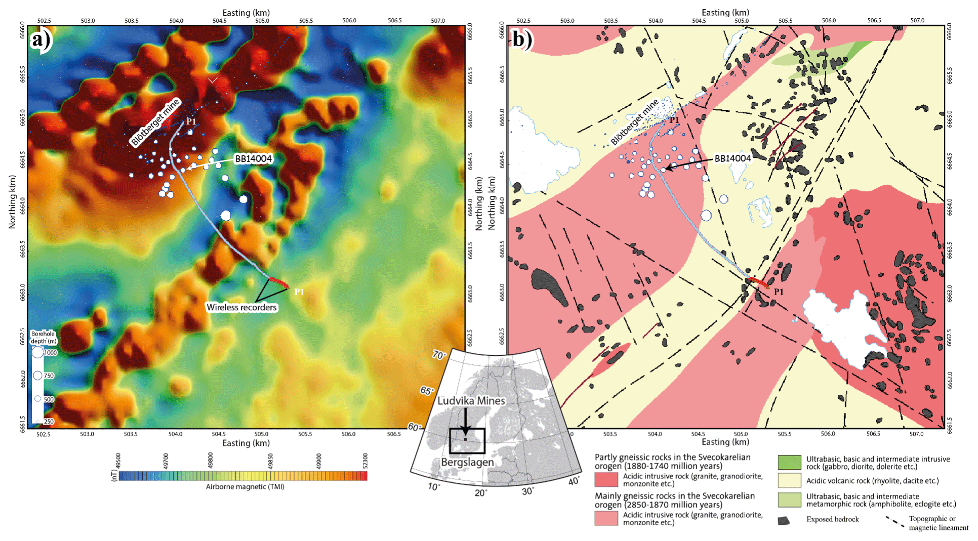
Figure 1(a) Total-field aeromagnetic and (b) geological maps of Blötberget within the Ludvika mines of the Bergslagen mineral district in central Sweden. A 2D seismic survey (blue line) and borehole BB14004 are used in this study. Magnetic data were provided by the Geological Survey of Sweden.
Due to dropping steel prices on the global market, mining operations had to be stopped in 1979. However, because of recent feasibility studies and more available resources, as well as the growing iron ore market, Nordic Iron Ore (NIO) plans to reopen the mine and exploit the deposits at a depth level of 400–420 m in the near future. Relevant to this study is the work by Maries et al. (2017) on a downhole logging study of the iron oxide deposits at the site. As shown in the logging data, the strong density contrast between the iron oxide deposits (∼ 4500 kg m−3) and their igneous host rocks (∼ 2500 kg m−3) should produce a strong impedance contrast as a good target for the seismic methods. However, the resistivity of the deposits is not as strong as normally expected for base metals (it is only on the order of 1000 Ω m) and very similar to that of the host rocks (around 3000–5000 Ω m) to make the resistivity-based methods (such as EM) suitable for depth delineation of deposits.
3.1 Review of the seismic data acquisition
The seismic survey was conducted along a 2D profile in 2016 (e.g. Markovic et al., 2020) following a feasibility study of a seismic land streamer survey (Malehmir et al., 2017). In order to better image the deposits, the seismic profile was designed to run approximately perpendicular to the strike of the known mineralized sheets. In the survey, 451 receivers were deployed (Fig. 1) of which 427 were cable-connected geophones (blue line) and 24 were wireless recorders (red line) deployed at the southern end of the profile. A 10 Hz spike-type geophone was used as the sensor. The cabled receivers were deployed approximately every 5 m and the wireless recorders approximately every 10 m. The source used was a 500 kg Bobcat-mounted drop hammer. The source locations were collocated with the receiver locations. The sampling rate was set as 1 ms and the recording time as 2 s. To avoid violating the 2D assumption of the subsurface below the seismic profile, we only use 369 receivers and sources that form a rather straight line in this study. The remaining 82 receivers and sources are not used due to the fact that they make a strong bend towards the north-west end of the profile. Details of the survey can be found in Markovic et al. (2020) and Maries et al. (2020).
3.2 Data pre-processing
The aim of data pre-processing is to strengthen the reflected events in terms of amplitudes and continuity. For the pre-processing of the seismic data, we designed a six-step workflow as shown in Fig. 2.
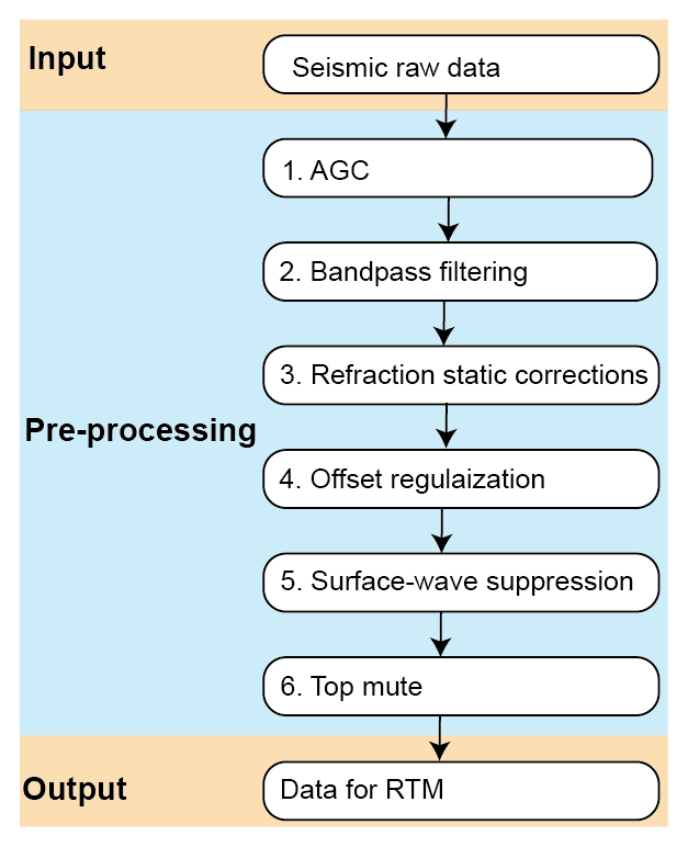
Figure 2The six-step data pre-processing workflow for the RTM imaging. In this study, offset regularization and surface-wave suppression had the most significant roles.
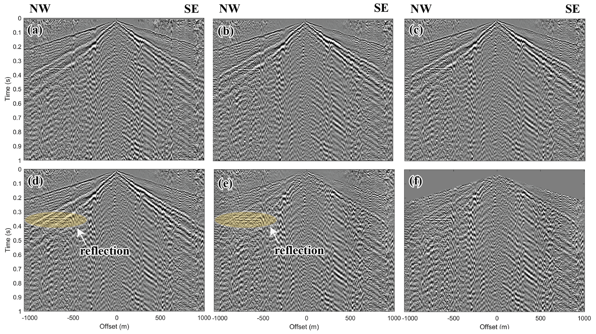
Figure 3(a) Example raw shot gather after AGC application (Step 1), (b) after bandpass filtering (Step 2), (c) after refraction static corrections (Step 3), (d) after data regularization (Step 4), (e) after surface-wave suppression (Step 5), and (f) after top muting (Step 6). The yellow ellipses mark a clear reflection, which we interpret to be from the iron oxide deposits.
Step 1. We applied automatic gain control (AGC) (e.g. Yilmaz, 2001) to balance the amplitudes at different offsets and different arrival times. The amplitudes of the raw data are more balanced after AGC (Fig. 3a). This step was necessary to reduce the strong amplitude of the surface waves relative to the weak reflection signals.
Step 2. We used a bandpass filter (10–35–150–200 Hz) to maintain data in this frequency band based on the analysis of the frequency band in the first breaks (Fig. 3b).
Step 3. We performed surface-consistent refraction static corrections to compensate for the near surface effects due to the different surface topography and the low-velocity glacial covers. The irregularity in the time of the first arrivals is mitigated after the refraction static corrections (Fig. 3c).
Step 4. We practised offset regularization of the dataset along a 1D smooth-curve line and obtained a regularized dataset (Fig. 3d). The original locations of sources and receivers (Fig. 4a) were projected onto the 1D curve, which was defined by a polynomial of degree 3 (Fig. 4b). Based on the projected receiver locations (Fig. 4c), we regularized the receiver spacing to a constant interval (i.e. 5 m) along the 1D curve (Fig. 4d). The seismic traces at those regularized receiver locations were obtained by a cubic interpolation using the traces at the projected receiver locations. Similarly, we regularized the source locations along the 1D curve and obtained the seismic traces every 5 m by a cubic interpolation, which was performed in the common receiver domain. After data regularization, we acquired the more even fold coverage required for RTM imaging. As a result, the total number of shot points (or receiver points) was regularized to 415 from the original 369. Such even fold coverage should contribute to an amplitude-balanced image, although one needs to use and inspect the interpolated seismic traces with care.
Step 5. We suppressed the surface waves (Fig. 3e) using the curvelet filtering method (Candès et al., 2006) on the regularized dataset. The geometrical difference of surface waves (almost linear events) and reflections (non-linear events) provides the feasibility to sperate them using curvelet filtering. After removing the strong surface waves with large amplitudes, the relative weaker reflection events show up clearly in the dataset. In the shown shot gather, the obvious reflection signal (yellow ellipse in Fig. 3e) has a small move out across offsets due to the specific source location relative to the dipping mineralization sheets.
Step 6. We muted the direct arrivals and the ambient noise above the first breaks (Fig. 3f) to reduce artefacts in the final seismic section.
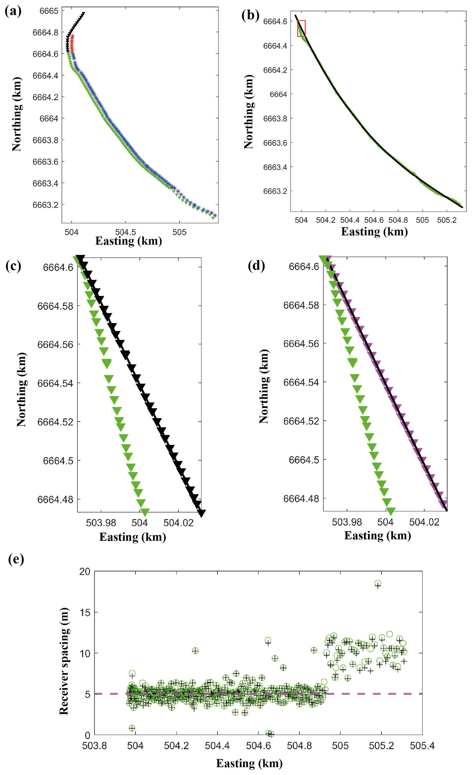
Figure 4(a) Original source (blue and red stars) and receiver (green and black triangles) locations. The blue sources and the green receivers were selected for RTM imaging. (b) The 1D smooth-curve line (black) based on a line-fitting method using the positions of green receivers. (c) The receivers (black triangles) projected along the 1D curve from their original locations (green triangles), zoomed on the red rectangle in (b). (d) The receivers (magenta triangles) regularized along the 1D curve from the projected receivers (black triangles) in (c). (e) The spacing of receivers in their original locations (green circles), their projected locations (black crosses), and regularized locations (magenta dashed line).
Note that we only used a bandpass filter to suppress parts of the noise. When forming an RTM image using the field data in the next section, the random noise in the data tends to be cancelled because of the cross-correlation imaging condition.
3.3 RTM imaging
The RTM imaging algorithm requires three ingredients: (1) a source wavelet, (2) a shot gather, and (3) a smooth but reasonable velocity model. Using the source wavelet and the migration velocity model, one can then forward propagate wave fields from the source side. Using the shot gather and the migration velocity model, the backward-propagating wave fields from the receiver side can then be modelled. Cross-correlation between the forward-propagating wave fields and the backward-propagating wave fields forms a partial RTM image from a single shot gather. During cross-correlation, an illumination compensation using source-side wave fields is done to balance the amplitudes in the seismic section (e.g. Valenciano and Biondi, 2003). Such a deconvolution imaging condition (Claerbout, 1971) removes the source wavelet approximately and hence improves the resolution of the image. The final RTM section is obtained by summing all the partial RTM images of all the shot gathers.
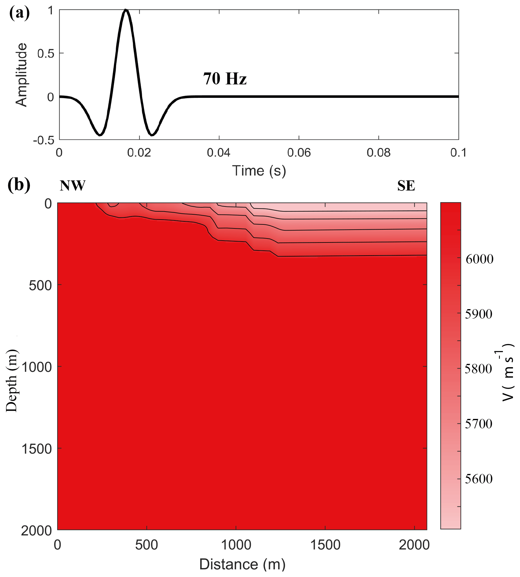
Figure 5(a) A Ricker wavelet (70 Hz) was chosen as the source wavelet, which generates forward propagating wave fields. (b) The migration velocity model used for the forward and backward propagations. The black lines are contour lines of the velocity values.
For the Blötberget seismic dataset, we used a staggered finite-difference modelling method (second order in time, fourth order in space) to realize the RTM. The source signal was chosen to be a Ricker wavelet (Fig. 5a) with a peak frequency of 70 Hz and a time step of s. The dt used in RTM is half of the sampling rate in the data. Hence, our data was up-sampled to dt by a linear interpolation before it was back-propagated. The 2D migration velocity consists of grids (Fig. 5b) of 401 (vertical) by 415 (horizontal) points. The grid interval was set to 5 m along both directions ( m). To obtain a good migration velocity model using this dataset, we performed the semblance velocity analysis (e.g. Zhou, 2014). By doing this, the reflected signal from the deposits was the main constraint. Thus, the velocity above the deposits were well constrained while the other areas are less constrained. To mitigate the numerical artefacts from the boundaries of the velocity model, we added perfectly matched layers (PMLs) (e.g. Komatitsch and Martin, 2007) on the four edges of the velocity model. Each PML has a thickness of 50 grid points. The wave field modelling had no free-surface effects due to the implemented PML.
We ran the RTM for all the 415 shot gathers to obtain 415 partial images. Then, we applied a Gaussian smoothing filter to suppress noise with small wavelengths ( m, i.e. two-grid size) in the partial images. Summing the smoothed 415 partial images, we obtained the final RTM image (Fig. 6). Using the dominant frequency (70 Hz) in the field data and the migration velocity (∼ 6000 m s−1) at depth, we estimated that the vertical resolution based on the major wavelength as approximately 100 m .
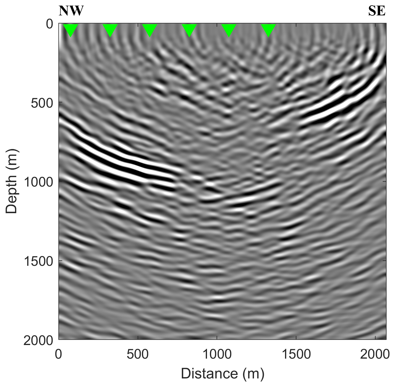
Figure 6Final RTM section of the Blötberget dataset. The green triangles are where common image gathers (CIGs) are shown later in the article.
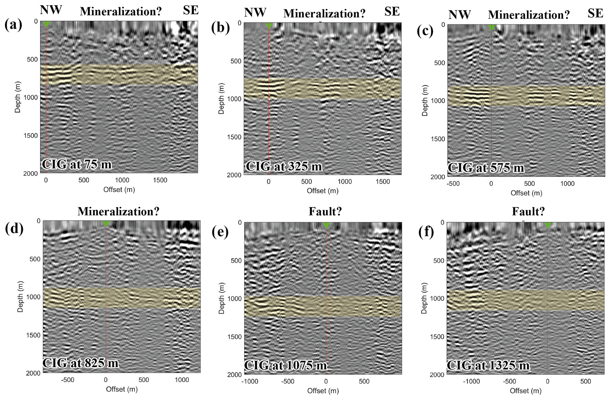
Figure 7Six CIGs at (a) 75 m, (b) 325 m, (c) 575 m, (d) 825 m, (e) 1075 m, and (f) 1325 m distances along the RTM section extracted to present the quality of the RTM section (see Fig. 5). The green receiver in each CIG collocates with their CIG positions in the original image. The yellow boxes highlight where the flat events are present.
Compared to the previous studies (Balestrini et al., 2020; Bräunig et al., 2020; Maries et al., 2020; Markovic et al., 2020) using the same dataset, the RTM image (Fig. 6) is much more promising in terms of imaging the crosscutting features and rock contacts. We validated the trustworthiness of the imaged reflectors in the RTM image in two ways. First, we analysed six common image gathers (CIGs) (e.g. Yan and Xie, 2011) from the image. Second, we integrated the results with other available geological and geophysical data to verify our interpretation of the reflectors in the section.
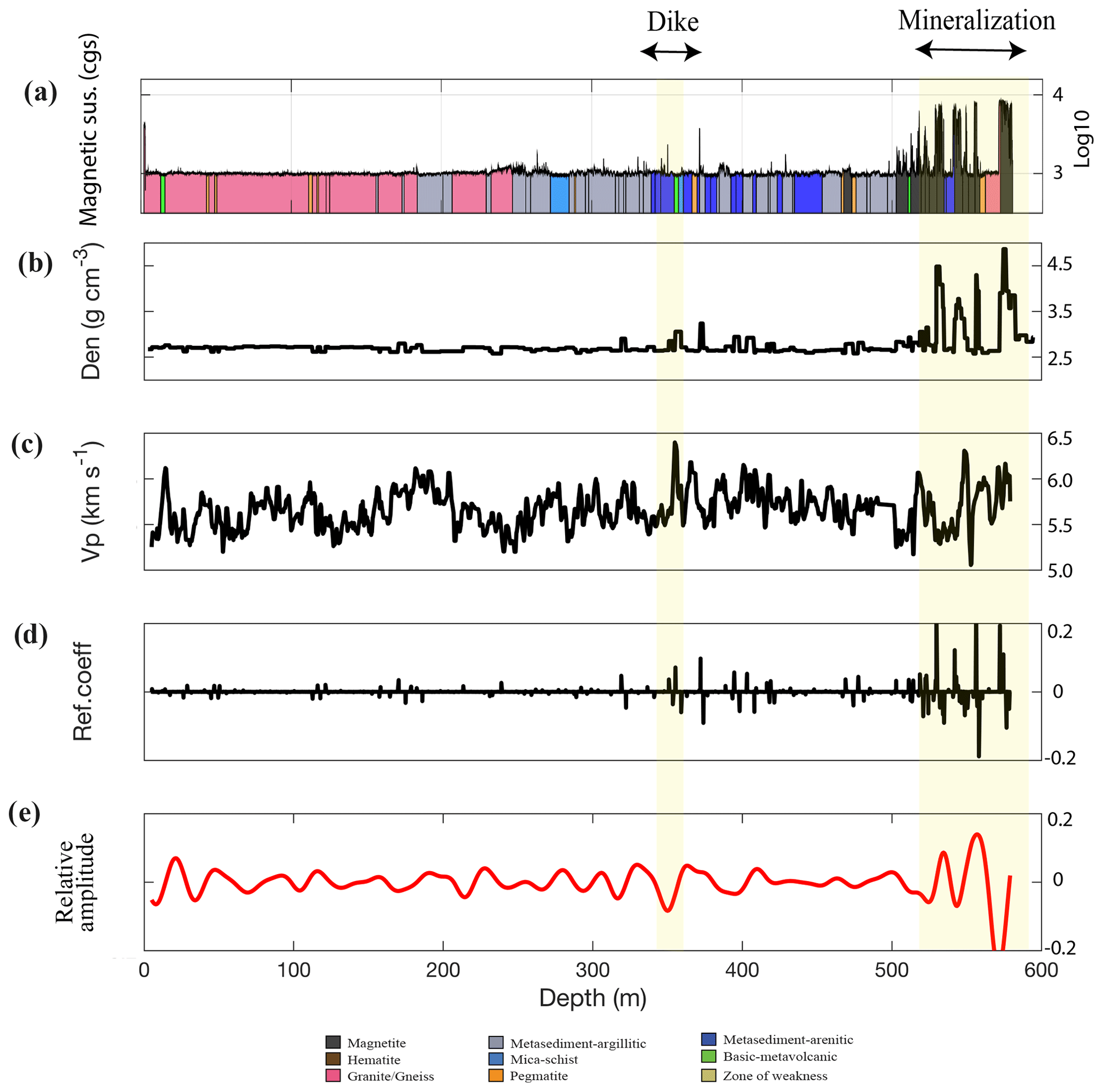
Figure 8Logging data from BB14004. (a) Natural gamma and rock types, (b) density, (c) P wave velocity values, and (d) calculated reflection coefficients. (e) The synthetic trace using a 70 Hz Ricker wavelet. The iron oxide deposits (530–570 m) produced a strong seismic signal in the synthetic trace.
For a trace in the final image (Fig. 6) at a specific spatial location (75, 325, 575, 825, 1075, and 1325 m distances along the profile), its corresponding common image gather (CIG) was formed by extracting the seismic traces from different partial images at the same spatial location. In our case, the CIG was composed of seismic traces extracted at those specific image locations from 415 single-shot partial images. In a single CIG gather, the traces were indexed by the offset between a source location and its specific CIG location in the RTM image. The flatness of continuous events in the CIG provided a qualitative evaluation of the fidelity of imaged reflectors. We extracted six CIGs from the RTM image (Fig. 6) at 75, 325, 575, 825, 1075, and 1325 m (Fig. 7). In the CIGs, the events reflected from the iron oxide deposits are quite continuous and flat (Fig. 7a–d) from zero offset to the far offset (∼ 900 m), while events reflected from the inferred faults (Markovic et al., 2020) do not show continuity across the whole section (Figs. 7e and 6f). The less continuous flattened events in the CIG corresponding to the inferred fault planes are likely due to the inaccuracy of the velocity model in the area of the inferred faults.
The CIGs only show the trustworthiness of the final seismic image in an image-wise sense. However, one should integrate these results with other geological and/or geophysical data to assist the interpretation of the seismic image. In our study area, four other datasets are available for this purpose. First, we have an existing 3D ore block model from boreholes. Second, two inferred 3D fault planes have recently been imaged and picked from a recent 3D survey (Malehmir et al., 2021). Third, one borehole (BB14004) near the seismic acquisition line has the natural gamma, core logging, density, and sonic logging data (Fig. 8) (Maries et al., 2017). Using the density data and P wave sonic data, we calculated their reflection coefficients (Fig. 8d) along the wellbore trajectories. Convolving the calculated reflection coefficients (Fig. 8d) with a 70 Hz Ricker wavelet, we obtained a synthetic seismic trace along the wellbore trajectory (Fig. 8e). Fourth, there are high-resolution (200 m flight spacing) aeromagnetic data (Fig. 9) available in this study area. The calculated magnetic anomaly data from the aeromagnetic data were used as well for the interpretation. Treating the RTM image as a dataset, we have five datasets in total. Assembling these five different datasets in 3D (Fig. 9), we can note their spatial relationships and correlations.
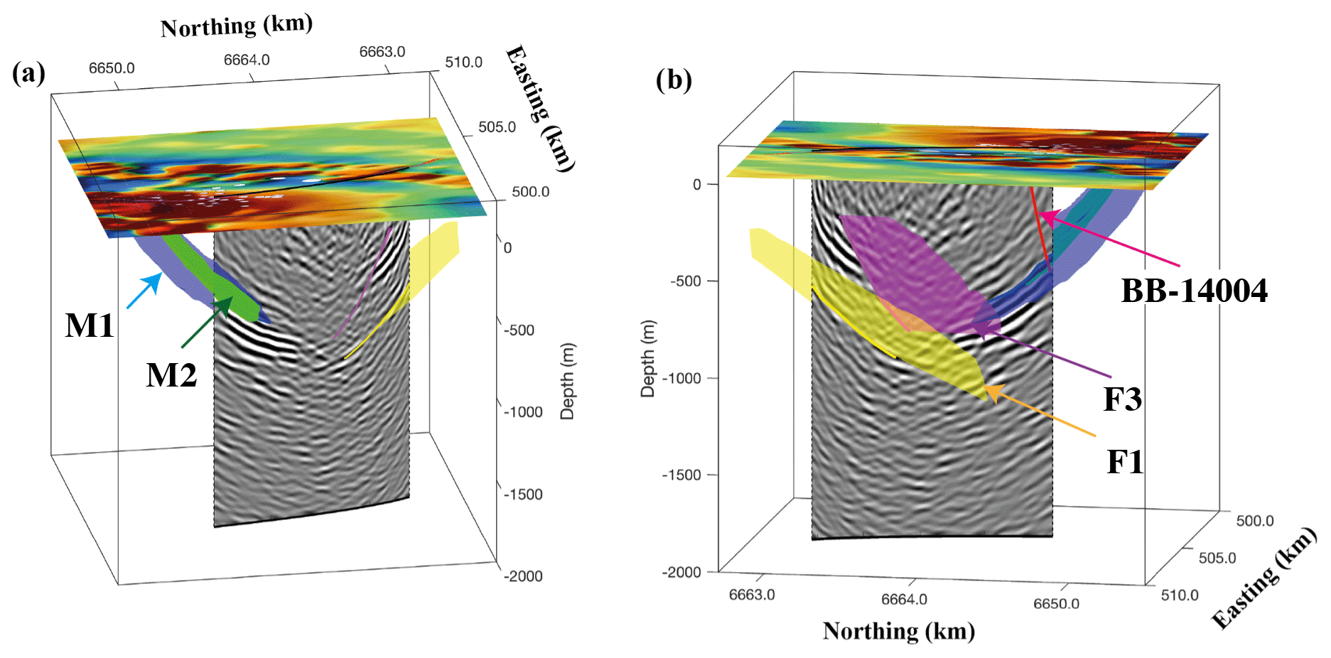
Figure 93D view integrating the RTM section with other geophysical data. (a) M1 and M2 are 3D ore block models intersecting the strong reflectors in the seismic section. These imaged strong reflectors also correlate well with the high magnetic anomaly seen on the northern part of the profile in the overlaid magnetic map. (b) Two inferred fault planes (F1 and F3) as mapped by the recent 3D seismic data in the area and borehole BB14004 (solid red line) intersecting the deposits. A small discrepancy between the imaged reflectors and the inferred fault planes (F1 and F3) might be due to the out-of-plane nature of these features producing a biased dip in the 2D RTM plane.
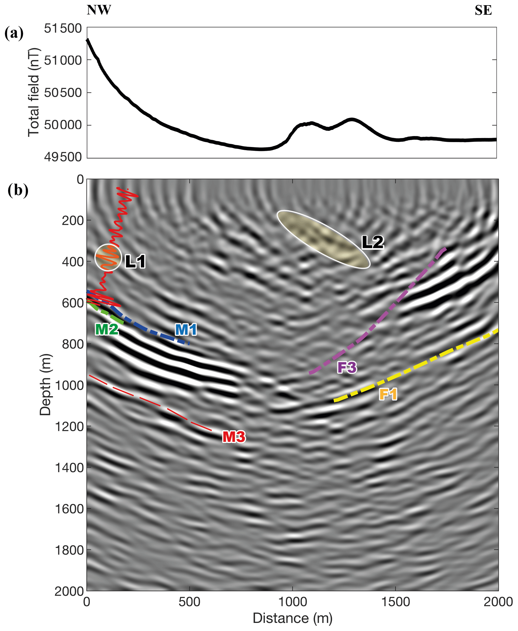
Figure 10(a) Total-field magnetic anomaly along the seismic section. (b) The intersections of two deposit surfaces (M1 & M2) and the intersection of the two fault planes (F1 & F2) are plotted. The synthetic trace is plotted along the well trajectory. R1 is interpreted to be from a lithological contact (see Fig. 8). R2 may be a weak iron oxide mineralization as it appears in a region with slightly higher magnetic properties than the neighbouring areas.
We interpreted the seismic image in the contexts of the four different datasets as mentioned above. For a better illustration, we also show the integrated datasets along the 2D seismic section (Fig. 10). First, we extracted the magnetic anomaly data along the seismic acquisition line (Fig. 10a). Based on the high values of the magnetic anomaly data in the north-east part along the profile, the position of the deposits is indicated well. From 1000 to 1500 m distance along the profile, the magnetic anomaly bulges up again, which we related to a shallow reflector (L2 in Fig. 10b) in the seismic section. Second, we plotted the intersections between the two mineralized sheets and the RTM image (M1 and M2 in Fig. 10b). The two intersection lines match well with the negative peaks in the seismic section. Based on the continuity of the reflectors at the deposit depths, it is highly reasonable that the mineralized sheets extend down to approximately 1000 m compared to the ore block model. We also marked M3 (Fig. 10b) as a potential mineralization below M1 and M2. Third, we marked out the intersections between the two inferred fault planes and the RTM image (F1 and F3 in Fig. 10b). The intersection due to the deeper fault (F1) matches well with the reflector, which crosscuts the deposit reflectors. However, the intersection due to the shallow fault (F3) only matches well with a reflector at the deeper part cutting through the deposits. Fourth, we projected the 1D synthetic seismic trace from BB14004 on the 2D image (Fig. 10b). The large amplitudes in the synthetic seismic trace at a depth interval of 500–600 m matches well with the reflectors in the image. Additionally, the reflector imaged above the deposits also matches well with weak amplitude in the synthetic seismic trace at a depth interval of approximately 350–370 m (L1 in Fig. 10b). We attributed this reflector to a dike (Fig. 8) based on the borehole core logging information. There are other reflectors clearly shown in the RTM image. However, we did not interpret them due to the lack of other geological and geophysical data at their locations.
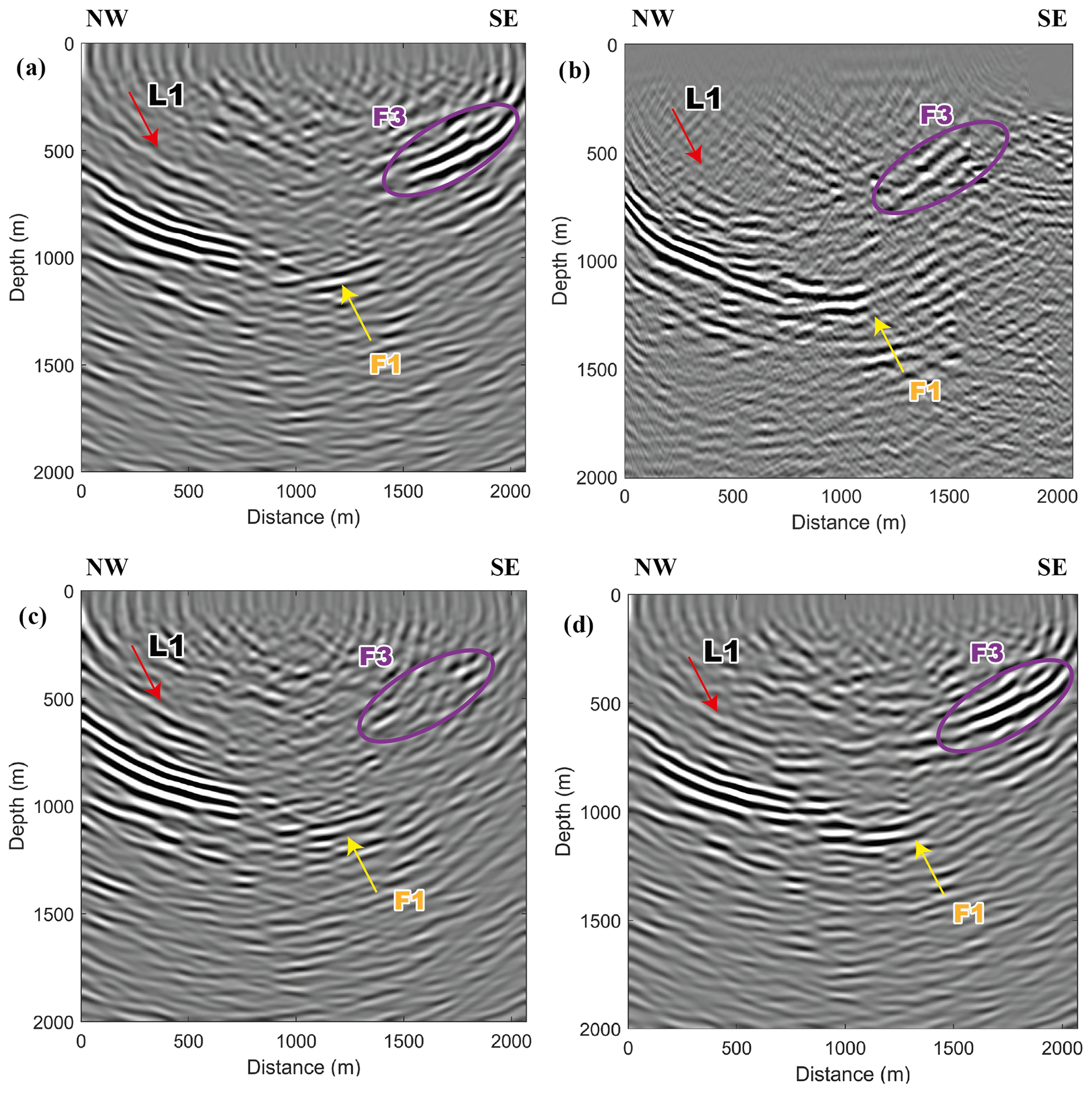
Figure 11Comparisons of different image results. (a) The RTM image (same as Fig. 10). (b) Image produced by a poststack Kirchhoff migration in Markovic et al. (2020). (c) RTM image obtained from data without offset regularization in the pre-processing (Step 4). (d) RTM image obtained from data with median filter applied in the pre-processing (Step 5).
A specific comparison was made between the produced RTM image (Fig. 11a) and the image (Fig. 11b) obtained by running a poststack Kirchhoff migration using two datasets acquired in 2015 and 2016 in the same area (Markovic et al., 2020). Though the main features of the mineralization are similar in the two images, the RTM section imaged one reflector (L1 in Fig. 11a) clearly above the mineralization and indicated well the two possible crosscutting features (F1 and F3 in Fig. 11a). Even though the RTM image was obtained using the dataset acquired in 2016 only, it showed more details because of the RTM imaging algorithm.
We also made comparisons of the RTM images produced from different datasets, which were pre-processed using different methods in the pre-processing flow. In this way, we demonstrated the influences of different pre-processing methods on the final RTM image results. To show the influence of the offset regularization (Step 4 in Fig. 2), we relocated the seismic traces in the original dataset to be at the points of 5 m grids along the 1D curve without trace interpolation. The relocation of any seismic trace was accomplished by moving the trace to the nearest point of the 5 m grids relative to its true receiver location. Keeping other pre-processing steps unchanged, the resultant RTM image (Fig. 11c) without offset regularization provided similar information as compared to the RTM image (Fig. 11a) obtained with offset regularization. However, the offset-regularized data improved fault imaging (ellipse in Fig. 11a) in the designed 10 m receiver-spacing area since the trace density was doubled in this area. To show the effects of different methods for surface-wave suppression (Step 5 in Fig. 2), we tested the widely used median filter to suppress the surface waves without changing other pre-processing steps. We found that the RTM section (Fig. 11d) obtained using the data pre-processed with median filter did not present the obvious crosscutting feature F1 that was shown in the RTM section (Fig. 11a) with the curvelet filter in the pre-processing.
In the current 2D case, when considering that the sheet-like targets have a dip at certain depth, one needs to set up the orientation and the length of the seismic line accordingly. The proper orientation (i.e. perpendicular to the strike of the targeted dipping layer) of the profile ensures obtaining a nearly true dip of the target in the image. The proper length of the profile allows receiving the reflected signal from the target at depth.
In our study, the six-step pre-processing workflow was essential in preconditioning the data and hence obtaining a good RTM seismic section. This pre-processing workflow is recommended for future studies of RTM on hardrock seismic data, though different methods could be used to pre-process the data as well. The migration velocity model is another factor that influences the accuracy of the resultant RTM image. If the data itself lacks reflection events to be used for good velocity analysis across the whole velocity model, one needs to be careful with the interpretation of the reflectors in the final image. With the CIG analysis (e.g. Schleicher et al., 2008), it is possible to refine the velocity model in future studies. Based on the flatness of those events in CIG images, we argue that the current velocity model works well for imaging the mineral deposits at the site, though the migration velocity needs to be updated to better image other subsurface structures. An accurate 2D velocity model using vertical seismic profiling (VSP) surveys could likely improve the RTM imaging results. However, the current study already supports the use of RTM imaging methods for hardrock seismic datasets and for mineral exploration purposes.
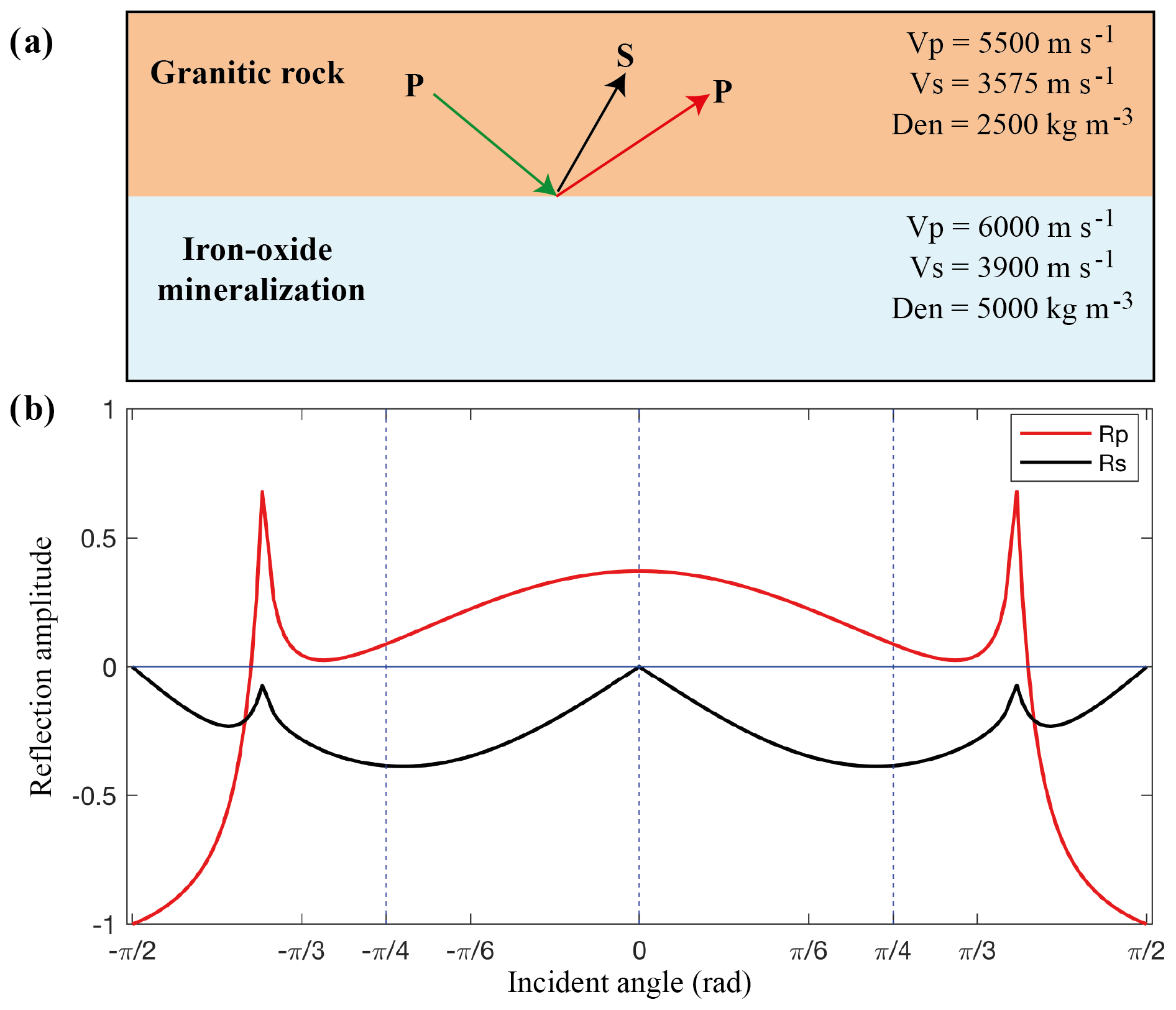
Figure 12(a) A two-layer model with rock properties of granitic rock in the top layer and that of iron oxide mineralization in the bottom layer. (b) The amplitude versus incident angle (AVA) response of the reflected P and S waves. The incident plane wave is a P wave with amplitude 1.
A remaining topic that one should also consider is whether there is a strong AVO or AVA (amplitude versus offset or amplitude versus angle) effect (Castagna and Backus, 1993; Hilterman et al., 2000) in the CIG images. Using Zoeppritz equations (Zoeppritz, 1919; Sheriff and Geldart, 1995), we calculated the AVA effect using a simple isotropic two-layer model (Fig. 12a), which simulates the physical properties of crystalline rocks. The amplitudes of P and S waves reflected from the horizontal contact between the granite and the iron oxide mineralization show a strong variation (Fig. 12b) versus the incident angles of the plane waves (P). Relevant to this specific dataset, the dipping angle and the thickness of the mineralized sheets need to be further accounted for when studying their AVO effects. Since the CIGs produced from the RTM partial images are ideal for studying the AVO effect relative to the CIG locations (Yan and Xie, 2012), future studies should exploit this potential for better scrutinizing and extracting physical property information from seismic data. Additionally, crystalline environments with a high degree of metamorphism may even show a strong anisotropic AVO response (Asaka, 2018). Utilizing the isotropic or anisotropic AVO analysis as a supplementary tool to characterize various rocks and mineral deposits from the seismic data is ideal in mineral exploration (Harrison and Urosevic, 2012).
We have studied the application of the RTM imaging method on a hardrock seismic dataset acquired for deep targeting iron oxide deposits in the Ludvika mining area of central Sweden. Using a six-step pre-processing workflow, we suppressed the unwanted noise and improved the signal-to-noise ratio. Consequently, the reflected events from the deposits and other geological features were remarkably strengthened. The resultant RTM image shows several reflectors, which are consistent when compared with four other independent datasets. From the known deposit model constrained by existing boreholes, two sets of strong seismic reflectors match well with the two iron oxide mineralized bearing horizons. Two oppositely dipping reflectors, interpreted to be from fault planes, intersect the two strong reflectors from the mineralization possibly implying a geological control on the extension or termination of these deposits at depth. Integrating the seismic image with the high-resolution magnetic anomaly data, a weak zone of iron oxide mineralization can be interpreted at shallow depth. Using P wave sonic data, density, and core logging data, we identified one continuous reflector as the dike formation.
The AVO effect was also studied using a simple two-layer model since we speculated a possible AVO response in the CIGs. There may be opportunities for detailed AVO studies of dense metallic deposits in either theoretical modelling or real field applications. In summary, using the Ludvika seismic dataset we demonstrate the usefulness of advanced imaging methods such as RTM for the deep targeting and imaging of mineral deposits and their host rock structures.
This work has benefited from the open-source software “CREWES” (https://www.crewes.org/ResearchLinks/FreeSoftware/, Margrave, 2020).
Original data underlying the material presented are available by contacting the corresponding author. However, as the dataset is the subject of other PhD studies, there is a 3-year embargo on their availability.
AM contributed to the data acquisition. YD worked on the data processing and wrote the paper, with contributions from AM.
The authors declare that they have no conflict of interest.
Publisher’s note: Copernicus Publications remains neutral with regard to jurisdictional claims in published maps and institutional affiliations.
This article is part of the special issue “State of the art in mineral exploration”. It is a result of the EGU General Assembly 2020, 3–8 May 2020.
This work was performed within the Smart Exploration project. The Smart Exploration was funded by European Union's Horizon 2020 research and innovation programme with the grant agreement no. 775971. We thank Nordic Iron Ore (NIO) AB for their collaboration in this study. Georgiana Maries is thanked for providing the density and sonic logs. We thank the three anonymous reviewers and the editor Ramon Carbonell for providing their helpful comments to improve the original version of the manuscript.
This research has been supported by the European Commission, H2020 Research Infrastructures (Smart Exploration (grant no. 775971)).
This paper was edited by Ramon Carbonell and reviewed by three anonymous referees.
Asaka, M.: Anisotropic AVO: Implications for reservoir characterization, Lead. Edge, 37, 916–923, https://doi.org/10.1190/tle37120916.1, 2018.
Balestrini, F., Draganov, D., Malehmir, A., Marsden, P., and Ghose, R.: Improved target illumination at Ludvika mines of Sweden through seismic-interferometric surface-wave suppression, Geophys. Prospect., 68, 200–213, https://doi.org/10.1111/1365-2478.12890, 2020.
Baysal, E., Kosloff, D. D., and Sherwood, J. W. C.: Reverse time migration, Geophysics, 48, 1514–1524, https://doi.org/10.1190/1.1441434, 1983.
Bednar, J. B.: A brief history of seismic migration, Geophysics, 70, 3MJ–20MJ, https://doi.org/10.1190/1.1926579, 2005.
Bellefleur, G., Cheraghi, S., and Malehmir, A.: Reprocessing legacy three-dimensional seismic data from the Halfmile Lake and Brunswick No. 6 volcanogenic massive sulphide deposits, New Brunswick, Canada1, Can. J. Earth Sci., 56, 569–583, https://doi.org/10.1139/cjes-2018-0103, 2018.
Bräunig, L., Buske, S., Malehmir, A., Bäckström, E., Schön, M., and Marsden, P.: Seismic depth imaging of iron-oxide deposits and their host rocks in the Ludvika mining area of central Sweden, Geophys. Prospect., 68, 24–43, https://doi.org/10.1111/1365-2478.12836, 2020.
Brodic, B., Kunder, R. D., Ras, P., Van den Berg, J., and Malehmir, A.: Seismic Imaging Using Electromagnetic Vibrators – Storm versus Lightning, European Association of Geoscientists & Engineers, 2019, 1–5, https://doi.org/10.3997/2214-4609.201902406, 2019.
Buske, S., Bellefleur, G., and Malehmir, A.: Introduction to special issue on “hard rock seismic imaging”, Geophys. Prospect., 63, 751–753, https://doi.org/10.1111/1365-2478.12257, 2015.
Candès, E., Demanet, L., Donoho, D., and Ying, L.: Fast Discrete Curvelet Transforms, Multiscale Model. Simul., 5, 861–899, https://doi.org/10.1137/05064182X, 2006.
Castagna, J. P. and Backus, M. M. (Eds.): Offset-dependent reflectivity – Theory and practice of AVO analysis, SEG, Tulsa, OK, USA, 1993.
Cheraghi, S., Malehmir, A., Bellefleur, G., Bongajum, E., and Bastani, M.: Scaling behavior and the effects of heterogeneity on shallow seismic imaging of mineral deposits: A case study from Brunswick No. 6 mining area, Canada, J. Appl. Geophys., 90, 1–18, https://doi.org/10.1016/j.jappgeo.2012.12.003, 2013.
Claerbout, J. F.: Toward a unified theory of reflector mapping, Geophysics, 36, 467–481, https://doi.org/10.1190/1.1440185, 1971.
Eaton, D. W., Milkereit, B., and Salisbury, M. H.: Hardrock Seismic Exploration, SEG, Tulsa, OK, USA, 2003.
Harrison, C. B. and Urosevic, M.: Seismic processing, inversion, and AVO for gold exploration – Case study from Western Australia, Geophysics, 77, WC235–WC243, https://doi.org/10.1190/geo2011-0506.1, 2012.
Hilterman, F., Van Schuyver, C., and Sbar, M.: AVO examples of long-offset 2-D data in the Gulf of Mexico, Lead. Edge, 19, 1200–1213, https://doi.org/10.1190/1.1438506, 2000.
Komatitsch, D. and Martin, R.: An unsplit convolutional perfectly matched layer improved at grazing incidence for the seismic wave equation, Geophysics, 72, SM155–SM167, https://doi.org/10.1190/1.2757586, 2007.
Magnusson, N. H.: The Origin of the Iron Ores in Central Sweden and the History of Their Alterations, Svensk reproduktions AB (distr.), 1970.
Margrave, G. F.: CREWES Matlab™ Toolbox and Textbook, CREWES [data set], available at: https://www.crewes.org/ResearchLinks/FreeSoftware/, last access: 1 October 2020.
Malehmir, A., Urosevic, M., Bellefleur, G., Juhlin, C., and Milkereit, B.: Seismic methods in mineral exploration and mine planning – Introduction, Geophysics, 77, WC1–WC2, https://doi.org/10.1190/2012-0724-SPSEIN.1, 2012a.
Malehmir, A., Durrheim, R., Bellefleur, G., Urosevic, M., Juhlin, C., White, D. J., Milkereit, B., and Campbell, G.: Seismic methods in mineral exploration and mine planning: A general overview of past and present case histories and a look into the future, Geophysics, 77, WC173–WC190, https://doi.org/10.1190/geo2012-0028.1, 2012b.
Malehmir, A., Maries, G., Bäckström, E., Schön, M., and Marsden, P.: Developing cost-effective seismic mineral exploration methods using a landstreamer and a drophammer, Sci. Rep.-UK, 7, 10325, https://doi.org/10.1038/s41598-017-10451-6, 2017.
Malehmir, A., Manzi, M., Draganov, D., Weckmann, U., and Auken, E.: Introduction to the special issue on “Cost-effective and innovative mineral exploration solutions”, Geophys. Prospect., 68, 3–6, https://doi.org/10.1111/1365-2478.12915, 2020.
Malehmir, A., Markovic, M., Marsden, P., Gil, A., Buske, S., Sito, L., Bäckström, E., Sadeghi, M., and Luth, S.: Sparse 3D reflection seismic survey for deep-targeting iron oxide deposits and their host rocks, Ludvika Mines, Sweden, Solid Earth, 12, 483–502, https://doi.org/10.5194/se-12-483-2021, 2021.
Maries, G., Malehmir, A., Bäckström, E., Schön, M., and Marsden, P.: Downhole physical property logging for iron-oxide exploration, rock quality, and mining: An example from central Sweden, Ore Geol. Rev., 90, 1–13, https://doi.org/10.1016/j.oregeorev.2017.10.012, 2017.
Maries, G., Malehmir, A., and Marsden, P.: Cross-profile seismic data acquisition, imaging and modeling of iron-oxide deposits: a case study from Blötberget, south central Sweden, Geophysics, 1–66, https://doi.org/10.1190/geo2020-0173.1, 2020.
Markovic, M., Maries, G., Malehmir, A., Ketelhodt, J. von, Bäckström, E., Schön, M., and Marsden, P.: Deep reflection seismic imaging of iron-oxide deposits in the Ludvika mining area of central Sweden, Geophys. Prospect., 68, 7–23, https://doi.org/10.1111/1365-2478.12855, 2020.
O'Brien, P. N. S.: Aspects of seismic reflection prospecting for oil and gas, Geophys. J. Int., 74, 97–127, https://doi.org/10.1111/j.1365-246X.1983.tb01872.x, 1983.
Pertuz, T., Malehmir, A., Bordic, B., Bäckström, E., Marsden, P., de Kunder, R., and Bos, J.: Broadband seismic data acquisition using an E-vib source for enhanced imaging of iron-oxide deposits, Sweden, in: Expanded abstracts, Society of Exploration Geophysicists, Houston, Texas, USA, 2020.
Schleicher, J., Costa, J. C., and Novais, A.: Time migration velocity analysis by image-wave propagation of common-image gathers, in: SEG Technical Program Expanded Abstracts 2008, 3133–3137, Society of Exploration Geophysicists, Las Vegas, Nevada, USA, https://doi.org/10.1190/1.3063997, 2008.
Sheriff, R. E. and Geldart, L. P.: Exploration Seismology, 2nd Edn., Cambridge University Press, Cambridge, 1995.
Ten Kroode, F., Bergler, S., Corsten, C., de Maag, J. W., Strijbos, F., and Tijhof, H.: Broadband seismic data – The importance of low frequencies, Geophysics, 78, WA3–WA14, https://doi.org/10.1190/geo2012-0294.1, 2013.
Valenciano, A. A. and Biondi, B.: 2-D deconvolution imaging condition for shot-profile migration, in: SEG Technical Program Expanded Abstracts 2003, 1059–1062, Society of Exploration Geophysicists, Dallas, Texas, USA, https://doi.org/10.1190/1.1817454, 2003.
Yan, R. and Xie, X.: Angle gather extraction for acoustic and isotropic elastic RTM, in: SEG Technical Program Expanded Abstracts 2011, 3141–3146, Society of Exploration Geophysicists, San Antonio, Texas, USA, https://doi.org/10.1190/1.3627848, 2011.
Yan, R. and Xie, X.: AVA analysis based on RTM angle-domain common image gather, in: SEG Technical Program Expanded Abstracts 2012, 1–6, Society of Exploration Geophysicists, Las Vegas, Nevada, USA, https://doi.org/10.1190/segam2012-0521.1, 2012.
Yilmaz, Ö.: Seismic Data Analysis, Society of Exploration Geophysicists, Tulsa, OK, USA, 2001.
Zhou, H.: Practical Seismic Data Analysis, High. Educ. Camb. Univ. Press, Cambridge University Press, New York, USA, https://doi.org/10.1017/CBO9781139027090, 2014.
Zhou, H., Hu, H., Zou, Z., Wo, Y., and Youn, O.: Reverse time migration: A prospect of seismic imaging methodology, Earth-Sci. Rev., 179, 207–227, https://doi.org/10.1016/j.earscirev.2018.02.008, 2018.
Zoeppritz, K.: VII b. Über Reflexion und Durchgang seismischer Wellen durch Unstetigkeitsflächen, Nachrichten Von Ges. Wiss. Zu Gött. Math.-Phys. Kl., 1919, 68–84, 1919.
- Abstract
- Introduction
- Study area
- RTM imaging on the Blötberget dataset
- RTM results, their interpretations, and comparisons
- Discussion
- Conclusions
- Code availability
- Data availability
- Author contributions
- Competing interests
- Disclaimer
- Special issue statement
- Acknowledgements
- Financial support
- Review statement
- References