the Creative Commons Attribution 4.0 License.
the Creative Commons Attribution 4.0 License.
 | 19 Aug 2021
Seismic radiation from wind turbines: observations and analytical modeling of frequency-dependent amplitude decays
Fabian Limberger
Michael Lindenfeld
Hagen Deckert
Georg Rümpker
In this study, we determine spectral characteristics and amplitude decays of wind turbine induced seismic signals in the far field of a wind farm (WF) close to Uettingen, Germany. Average power spectral densities (PSDs) are calculated from 10 min time segments extracted from (up to) 6 months of continuous recordings at 19 seismic stations, positioned along an 8 km profile starting from the WF. We identify seven distinct PSD peaks in the frequency range between 1 and 8 Hz that can be observed to at least 4 km distance; lower-frequency peaks are detectable up to the end of the profile. At distances between 300 m and 4 km the PSD amplitude decay can be described by a power law with exponent b. The measured b values exhibit a linear frequency dependence and range from b=0.39 at 1.14 Hz to b=3.93 at 7.6 Hz. In a second step, the seismic radiation and amplitude decays are modeled using an analytical approach that approximates the surface wave field. Since we observe temporally varying phase differences between seismograms recorded directly at the base of the individual wind turbines (WTs), source signal phase information is included in the modeling approach. We show that phase differences between source signals have significant effects on the seismic radiation pattern and amplitude decays. Therefore, we develop a phase shift elimination method to handle the challenge of choosing representative source characteristics as an input for the modeling. To optimize the fitting of modeled and observed amplitude decay curves, we perform a grid search to constrain the two model parameters, i.e., the seismic shear wave velocity and quality factor. The comparison of modeled and observed amplitude decays for the seven prominent frequencies shows very good agreement and allows the constraint of shear velocities and quality factors for a two-layer model of the subsurface. The approach is generalized to predict amplitude decays and radiation patterns for WFs of arbitrary geometry.
- Article
(12300 KB) - Full-text XML
-
Supplement
(600 KB) - BibTeX
- EndNote


In recent years, debates on the emission of seismic waves produced by wind turbines (WTs) and its potential effects on the quality of seismological recordings have led to increased research efforts on this topic. The main objectives are the characterization of WT-induced seismic signals, the definition of protection radii around seismological stations, and the modeling-based prediction of WT effects on seismological recordings in advance of the installation of WTs. Styles et al. (2005) reported about discrete frequency peaks in seismic noise spectra that increase with wind speed and the rotation rate of a nearby WT and assigned the observed peaks to vibration modes of the WT tower and rotor rotation. Zieger and Ritter (2018) and Stammler and Ceranna (2016) confirmed discrete frequency peaks between 1 and 10 Hz and analyzed signal amplitude decays with distance to the WTs described by a power law. Saccorotti et al. (2011) observed seismic signals with a frequency of about 1.7 Hz that were associated with WTs at distances of up to 11 km. Friedrich et al. (2018) used a migration analysis to identify seismic signals from nearby wind farms (WFs) and were able to distinguish between various WFs based on differences in frequency content. Polarization analyses was used by Westwood and Styles (2017) to show that Rayleigh waves dominate the wave field emitted from WTs. This observation was confirmed by numerical simulations (Gortsas et al., 2017). The increase of the noise amplitude with the square root of the number of WTs () was observed by Neuffer et al. (2019) based on WT shutdown tests. Lerbs et al. (2020) proposed an approach to define protection radii, e.g., 3.7 km around the Collm Observatory (CLL) in Germany, using a power law to describe the spatial wave attenuation. Furthermore, the ground motion polarization near a single WT was analyzed and provided insights into the interaction of WT nacelle movement and emitted seismic signals.
Approaches to model the seismic radiation from WTs are rare and focus mostly on modeling the ground vibration of a single WT (Gortsas et al., 2017) or its operational components only (e.g., Zieger et al., 2020) but not on wave field propagation considering superimposed wave fields and amplitude decay with distance to multiple WTs simultaneously. However, Saccorotti et al. (2011) used an analytical approach to model the observed amplitude decays by summing up the calculated noise amplitudes produced by several WTs, including an intrinsic attenuation law, but they did not study possible effects of multiple WTs on the interference of the emitted wave fields.
In this paper, we present an analytical approach to model frequency-dependent seismic radiation and amplitude decays with distance in comparison to robust long-term observed decay curves, measured at a WF in Uettingen (Bavaria, Germany). In a first step, we derive distance-dependent noise spectra from recordings of up to 6 months in duration and characterize the relation between signal frequency and amplitude decay. We face the challenge of handling phase differences between multiple source signals that have strong effects on the seismic radiation due to significant changes in interference pattern of the superimposed wave fields. We apply the phase shift elimination method (PSE method) to generate representative source signals as an input for the analytical modeling of the observed amplitude decays. The comparison between modeled and observed amplitude decays also allows the constraining of the parameters of a simple two-layer model of the subsurface. We further show how it is possible to generalize the approach to predict radiation patterns for arbitrary WF geometries.
Our surveys were conducted in the neighborhood of a WF in Uettingen, about 9 km west of Würzburg in Bavaria. The WF consists of three WTs positioned in a NW–SE line with a spacing of 350 m and 450 m, respectively. The Nordex N117 type WTs have 2400 kW rated power and a tower height of 141 m. Their maximum rotation rate is about 12 rpm (rotations per minute). To measure the amplitude decay of the seismic WT signals we deployed 19 seismic stations along a profile of 8.3 km length, starting at the easternmost of the three WTs and running in NE direction approximately perpendicular to the geometrical layout of the WF (Fig. 1). Additionally, we placed three stations in the WT basements in order to record the seismic source signal of each WT. The instruments were installed between July and November 2019, and data recording will extend until August 2021. All stations are equipped with Trillium Compact posthole sensors (20 s) and Centaur data loggers (Nanometrics) recording continuously at a sampling frequency of 200 Hz. To improve the signal and noise conditions the sensors of the profile stations were placed in shallow boreholes of 1–2 m depth.
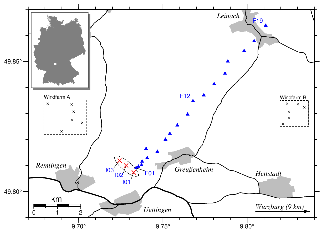
Figure 1Location of the wind farm in Uettingen (red crosses) and seismic profile stations F01 to F19 (blue triangles). Three additional seismic stations are positioned in the WT cellars (I01, I02, I03). Wind farms A and B (dashed boxes) are not targeted by our experiment but are located in the area.
The local near-surface geology is defined by Triassic sedimentary rocks. Beneath a thin soil layer, limestones of the Muschelkalk are situated over clastic sediments of the Buntsandstein, mainly terrestrial quartzite, sandstone, and claystone layers. Geologic cross sections suggest that the lower Muschelkalk under the topographic surface reaches a thickness of up to several tens of meters (Bayerisches Geologisches Landesamt, 1978). However, at some seismic stations the Muschelkalk–Buntsandstein boundary is only a few meters below the surface. In topographic depressions the Muschelkalk can be completely missing, i.e., thin quaternary soft sediments directly cover Upper Buntsandstein rocks.
2.1 Calculation of average power spectral densities (PSDs)
We analyzed a continuous dataset between September 2019 and March 2020, covering a range of 159 to 207 d depending on the exact station installation date. We associate the measured amplitudes in the seismic waveform data with the corresponding WT parameter (in this case “rotor speed”) at a resolution of 10 min. For this reason, the recordings of each profile station were split into 10 min segments that were transformed to power spectral density spectra using the method of Welch (1967). Each of these spectra were then sorted according to the respective rotor speed into bins of 1 rpm width. With this procedure we generated close to 10 000 single PSDs within the bin of maximal rotor speed (11–12 rpm) called “full power” status for each station, and about 2000 single PSDs for the “zero power” status of the WT (0–1 rpm). In order to reliably remove outliers and reduce the impact of local transient noise (e.g., traffic on nearby roads), we excluded 75 % of the largest PSD amplitudes and used only 25 % of the single PSDs to calculate the final average PSD spectra. This seems to be a relatively strong limitation of the dataset. However, due to the long observation period there are still enough data left to calculate robust average spectra. We think that this approach provides a reliable and conservative estimate of the spectral WT amplitudes with a minimized influence of interfering transient signals. Figure S1 in the Supplement illustrates the influence of different percentiles on the calculated average PSD at station F01.
Figures 2 and 3 show the resulting average PSDs (25 % percentile) for the full power and the zero power WT status, respectively. Besides the strong microseismic peak at about 0.2 Hz, we identified nine peaks of significant energy centered at 1.14, 1.7, 2.3, 3.5, 4.8, 6.0, 7.6, 10.5, and 17.2 Hz. All of them show a systematic amplitude decrease with increasing station distance, indicating that their origin is located at the WT. For peaks 1 to 7 we fitted the observed amplitude decay with a power law model (see next section). Because of the rapid amplitude decay at frequencies >10 Hz, we were not able to reliably fit peaks 8 and 9. For comparison we show the respective average PSDs recorded during zero power status (0–1 rpm) in Fig. 3. In this case the observed spectral peaks 1 to 9 have completely disappeared. The remaining (sharp) peaks show no systematic dependence with distance to the WF or the rotation rate of the WTs, which is an indication that their origin is not related to the WTs. High-frequency signals at >4 Hz have a large amplitude in the near field only. Similar peak distributions have been observed by Neuffer et al. (2019) and Lerbs et al. (2020).

Figure 2Average PSD spectra at full power status (11–12 rpm), calculated at profile stations F01 to F16 in the time range from September 2019 to March 2020. The distance of each station to the WT is color coded and indicated in the figure legend. In total, nine energy peaks are identified between 1.14 and 17.2 Hz, all of which show a systematic amplitude decrease with increasing station distance. The amplitude decays of peaks 1 to 7 have been measured and fitted by a power law.
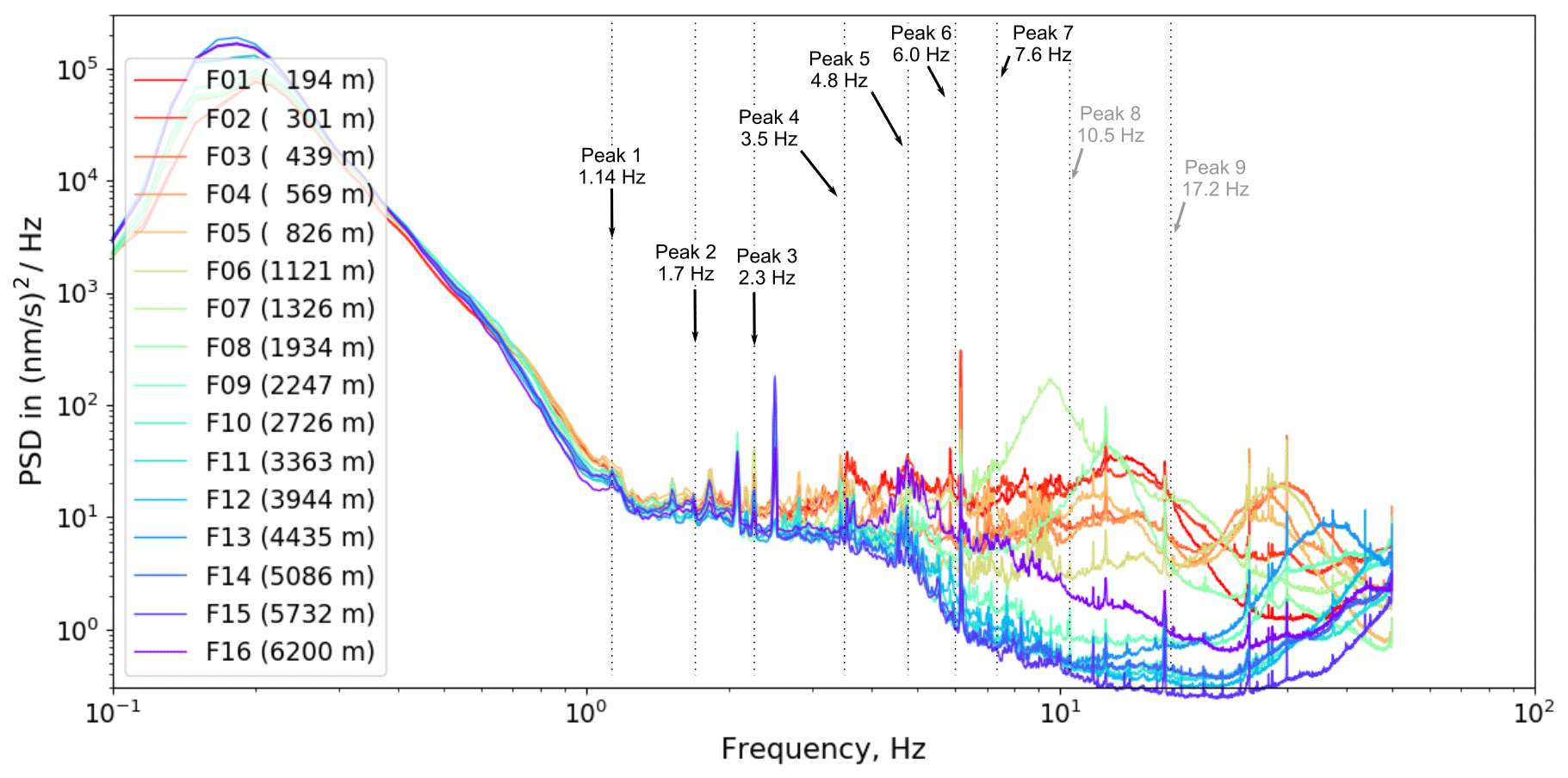
Figure 3Average PSD spectra at zero power status (0–1 rpm), calculated at profile stations F01 to F16 in the time range from September 2019 to March 2020. The identified peaks at full power (Fig. 2) have disappeared. The remaining sharp peaks show no systematic decrease with increasing distance, indicating that they have a different origin.
2.1.1 Power-law fitting of the observed amplitude decay
To quantify the PSD amplitude decay, the respective peak maxima of the full power PSDs (Fig. 2) were picked at each station. Figure 4 shows the resulting attenuation curves for peak 1 (1.14 Hz) to peak 7 (7.6 Hz) using a double-logarithmic representation, i.e., the logarithm of peak amplitude is shown versus the logarithm of the station distance. If the PSD amplitude decay corresponds to a power law, which is the basic assumption, there should be a linear correlation between log(amplitude) and log(distance). The attenuation factor, b, can then be calculated as the slope of a linear fit of the attenuation curves. As Fig. 4 shows, the measured PSD amplitude decays can be described in good approximation with a power law between station F02 and F12, which corresponds to a distance range of 300 to 4000 m. Beyond F12, the measured PSD amplitudes increase with larger distances, except for peak 1 (1.14 Hz), and it was not possible to identify clear peak maxima, since the background noise dominates the spectra. Towards the end of the seismic profile the stations get closer to a high-speed railway track and populated areas with raised ambient noise conditions, which might explain the observed excessive PSD amplitudes in this region. However, the first two stations of the profile – F01 (194 m) and F01a (239 m) – also show deviations from a power law attenuation. Due to the proximity of these stations to the WT, the amplitudes may also be affected by near-field effects.

Figure 4Double logarithmic representation of PSD amplitude decay at seven different peak frequencies. Blue circles mark the measured amplitudes from station F01 (194 m) to station F19 (8413 m) at full power status of the WT. Filled symbols denote data points that were used for power law fitting (red lines) between station F02 (301 m) and F12 (3944 m) with attenuation factor b and correlation coefficient R2.
For these reasons we decided to restrict the analysis of the amplitude decay to the distance range between 300 and 4000 m and to estimate the attenuation factor, b, using a linear least-squares fit between station F02 and F12 for all seven peak frequencies. The results show a systematic increase with frequency and yield values from b=0.39 at 1.14 Hz up to b=3.93 at 7.6 Hz. In Fig. 5 we show the frequency dependence of the attenuation factor b. It exhibits a nearly perfect linear relationship between b and frequency, at least within the analyzed frequency range from 1.14 to 7.6 Hz. The comparison to results from other authors is discussed below (Sect. 5).
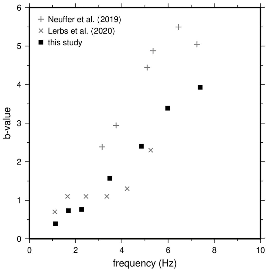
Figure 5Frequency dependence of b values for peak 1 to peak 7 (filled symbols, cf. Fig. 4). Plus signs and crosses mark calculated b values of Neuffer et al. (2019) and Lerbs et al. (2020), respectively.
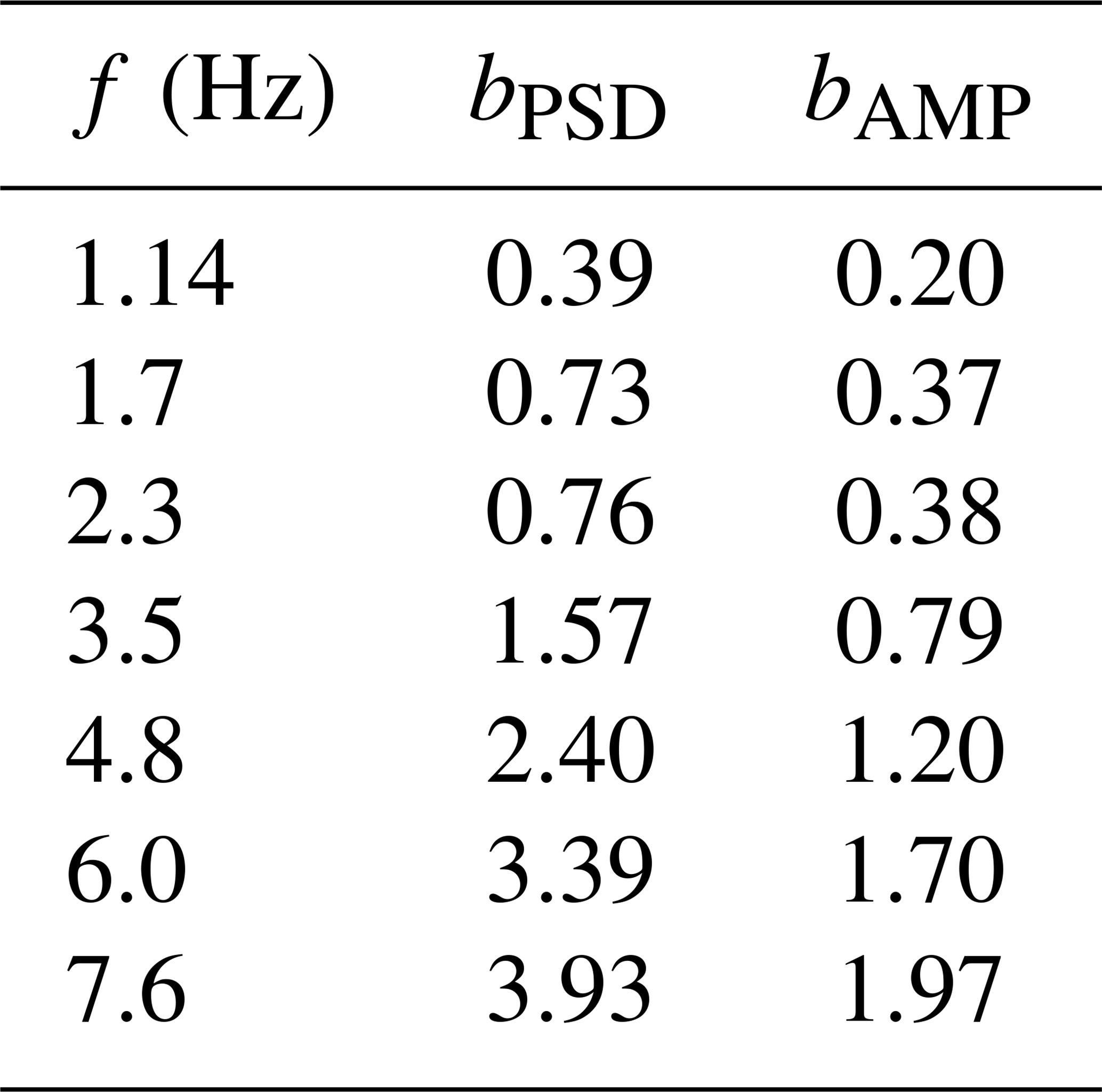
The b values quantify the decay of PSD peaks in the vicinity of the Uettingen wind farm. Since PSD amplitudes are proportional to the square of amplitudes in the time domain it is possible to estimate the corresponding b values for time signals by applying a factor of 0.5. Table 1 lists both types of attenuation factors: bPSD for the PSD decay, and bAMP for the corresponding time amplitude decay. This should enable a better classification of our results.
Table 1Calculated b values for the PSD amplitude decay, bPSD, and corresponding b values of the signal amplitude decay, bAMP. The latter was derived from bPSD by the application of factor 0.5.
2.2 Observation of phase shifts between multiple WT vibrations
Each WT can be considered a seismic source. By analyzing the seismograms measured simultaneously in the three WTs (I01, I02, and I03) of the WF Uettingen, we observe phase shifts between the individual wave forms (Fig. 6a). As an example, three time series (vertical component), each recorded in one of the WT cellars during a rotation rate of about 11.5 rpm, are filtered to a narrow bandwidth around frequency peak 1 with 1.14 Hz (1.10–1.18 Hz) and are compared within a time window of 22 s. In the first 2 s, the signal phase of seismic station I03 is shifted by π compared to signal I01 and I02, which are in phase. Between 10 and 13 s, all signals are almost in phase, which consequently means that the WTs are vertically vibrating in phase. After 15 s, all three signals are shifted to each other and are not in phase anymore. For a longer time period of 1 h, the phase shifts between signals measured at I01 and I02 are determined using a cross-correlation analysis with a moving time window of 5 s (=720 time segments) along the 1 h time segment. The temporal shift is converted to the corresponding phase shift between −π and π for each window. The distribution of all 720 resulting phase shifts is almost uniform (Fig. 6b) and shows no systematic behavior with time (Fig. 6c), which leads to the conclusion that phase differences between source signals appear rather randomly, especially over longer time periods.

Figure 6(a) Comparison of seismograms (vertical components) measured simultaneously in each of the three WTs at a rotation rate of 11–12 rpm. Waveforms are filtered to 1.10–1.18Hz, and amplitudes are normalized to their maximum. (b) Distribution of phase shift between signals in 5 s time segments measured in two WTs (I01 and I02) during a period of 1 h with WT rotation rates of 11–12 rpm. (c) Temporal development of the phase shift between the signals measured in the two WTs (I01 and I02).
In the following section, we model the observed amplitude decays and set up a mathematical formulation that includes a source function, attenuation factors, geological properties, and the superposition of multiple wave fields (produced by multiple WTs). In view of the observation that the source signals of neighboring WTs are not in phase, we study the influence of possible signal phase differences on the amplitude decay and propose a solution as to how to account for or “eliminate” this effect in the calculation.
3.1 Surface wave field approximation
Previous research suggests that mainly vertically polarized Rayleigh waves are emitted from WTs and that they dominate the WT-induced seismic noise (Westwood and Styles, 2017; Neuffer and Kremers, 2017; Gortsas et al., 2017). However, recent studies indicate that both Rayleigh and Love waves are emitted from WTs (see Lerbs et al., 2020; Neuffer et al., 2021). In our models, we assume that surface wave amplitudes decay proportionally to (with distance r to the source) due to geometrical spreading of the surface wave front on a cylindrical area in the 2D surface plane
where r0 is a reference (minimal) distance (Bugeja, 2011).
Geometrical spreading is independent of wave frequency. In addition, attenuation due to intrinsic absorption reduces the wave amplitude with distance to its source
The damping factor, D, depends on frequency w=2πf, seismic wave velocity c, and again the travel distance r of the wave (Bugeja, 2011). Furthermore, D is a function of the seismic quality factor Q, which describes the loss of energy per seismic wave cycle due to anelastic processes or friction inside the rock during the wave propagation. The damping of the wave is decreasing with increasing Q. The source signal S(t) itself is approximated by a continuous periodic cosine-function to simulate the periodic motion at the base of the WT in vertical direction
where S(t) is a function of time t, signal frequency w=2πf, amplitude calibration factor A, wave number , and signal phase Φ.
Assuming a homogeneous half-space, the wave amplitude can be calculated for any distance r to the source (Fig. 7). Considering N source points (WTs), the amplitude at each point and hence the total wave field is derived by summation over all N wave fields
where index i corresponds to source point i and the relative radial distance to the source points is given by . Shear quality factor QS and seismic shear wave velocity cS are model parameters and define the properties of the material the wave is traveling through. Z(t) is the superposition of the individual wave fields and can be calculated at any time t.
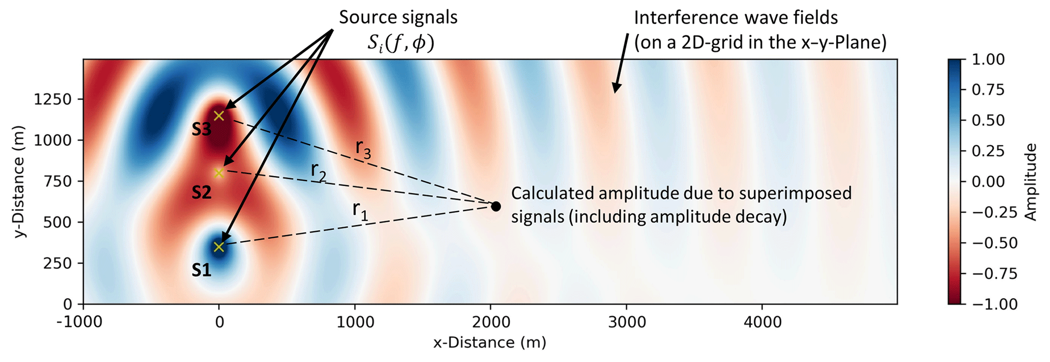
Figure 7Schematic figure of the analytical modeling approach. Amplitudes as functions of time are calculated at points (x, y).
By modeling the interference wave field as a function of time, this approach allows to derive root-mean-square amplitudes (rms amplitudes) at any point at the surface. For the calculation, the amplitude calibration factor Ai will be set to 1 for every source signal, since all three WTs of the Uettingen WF are of the same type. It should be noted that body waves (P, S) are not considered in this modeling approach, since the simulated wave field approximates a wave field dominated by Rayleigh waves. The velocity of Rayleigh waves cR is generally slightly lower than the shear wave velocity cS, whereas the ratio depends on the Poisson ratio ν (e.g., Rahman and Michelitsch, 2006). Assuming theoretical values of ν from 0.0 to 0.5, the ratio can reach values between 0.87 and 0.95 (Leiber, 2003; Hayashi, 2008), which means that the Rayleigh wave velocity is maximally about 13 % lower than the shear wave velocity. However, it is possible to approximate surface wave fields using the shear wave velocity (Kumagai et al., 2020). The penetration depth of Rayleigh waves, which is influenced by the physical properties of near-surface geological layers and the wavelength, plays an important role in approaching the modeling of WT-induced seismic wave propagation. The correct quantification of the penetration depth of Rayleigh waves is widely studied; however, so far there is no general consensus on their penetration depth in relation to the seismic wavelength λ. Based on results of Hayashi (2008), Kumagai et al. (2020) claim that surface wave velocity reflects the average S-wave velocity of the geological layers down to a depth between and , whereas is often chosen to be the most suitable assumption (e.g., Larose, 2005). Moreover, it is common to derive depth information from observed wave attenuation applying modeling or tomography methods to seismological data (e.g., Siena et al., 2014). Due to Rayleigh wave dispersion, it is known that low-frequency surface waves reach deeper into the subsurface and thus will travel through materials with likely higher Q and seismic velocities c. Consequently, the damping is reduced compared to high-frequency surface waves (Karatzetzou et al., 2014; Farrugia et al., 2015). Taking this into account, we use the following relation for wavelength depth conversion
In this study, we take advantage of the link between frequency-dependent amplitude decays (depending on QS and cS, Eq. 4) and surface wave penetration depth to derive information about shear wave velocities and quality factors in the subsurface (Eq. 5).
3.2 Effect of source-signal phase on seismic radiation and amplitude decay
Since we observe significant changes of the phase shifts between signals measured at the three WTs (Sect. 2.3), we aim to study its effect on the wave field that is emitted by the three WTs in Uettingen. Hence, three wave fields are calculated using three different source phase compositions assuming a 1.14 Hz source signal frequency, 1500 m s−1 wave velocity and equality factor of 30 as an exemplary model. Source points are located at m and y1=350 m, y2=800 m, and y3=1150 m (Fig. 7). Amplitudes are calculated along a profile extending from source signal S1 (see Fig. 7) and perpendicular to the WF line, which approximates the real geometry of the WF and seismic profile in Uettingen. The results show a clear dependence of the amplitude decays on the source signal phase composition (Fig. 8). In addition, amplitudes at the end of the 5000 m long profile differ significantly from each other. In the third scenario (Fig. 8c), the expected amplitude is a quarter of the amplitude that is reached if the WTs are vibrating in phase (Fig. 8a). Furthermore, strong effects appear in the first 2 km of the profile. Scenario (a) shows increased amplitudes due to constructive wave interference in the near field, whereas scenario (c) indicates a rapid decay of amplitudes within the first 1000 m of the profile. Scenario (b) shows a smoother and steadier decay of the amplitudes and reaches an amplitude at the end of the profile that is reduced by a fifth compared to scenario (a). These exemplary scenarios demonstrate only three out of infinite possibilities of different source signal phase compositions. Taking this into account, the seismic radiation of a WF is affected by phase differences of the source signals which can lead to strong changes in the wave field interference.
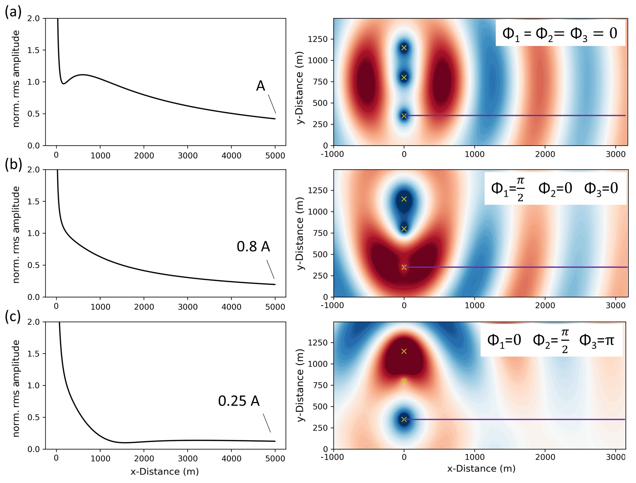
Figure 8Calculated amplitude decay curves (in the direction of the magenta line) for three scenarios with different source signal phase compositions using (a) (vibration in phase), (b) , Φ2=0, Φ3=0, and (c) Φ1=0, , Φ3=π. Index 1 represents the source point S1. All decay curves are normalized to the amplitude at x=300 m.
3.3 Phase shift elimination and data fitting
In this section we propose a method of how to handle the observed time-varying source signal phases and their effect on the seismic radiation using the assumption of a random appearance of signal phase constellation of multiple WTs, especially regarding long time periods. To define representative source signals, we developed a phase shift elimination method (PSE method). Within this PSE method, 500 radiation patterns (i.e., wave fields) are calculated using random signal phases Φ (between 0 and π) for each individual source signal. All 500 calculated wave fields are then averaged, and the average amplitude decay is extracted along the profile, which in turn is independent of the individual source signal phases. We experienced that the wave field averaging process and hence final amplitude decay calculation is sufficiently stable after 500 wave field simulations, whereas a number of <100 seems too low to generate a reproducible result. We apply this method to the Uettingen WF setup and compare the modeling results with the observed amplitude decays in Uettingen during rotation rates between 11 and 12 rpm (all WTs under full power). Since the observed PSD amplitudes are proportional to squared ground motion amplitudes in the time domain (rms amplitudes), we compare our modeling results (rms amplitudes) with the square root of the observed PSD amplitudes. The analysis is performed for signals with center frequencies of 1.14, 1.69, 2.26, 3.5, 4.85, 5.98, and 7.6 Hz, representing the 7 PSD peaks in Uettingen (see Sect. 2.1). For comparison, all decay curves are normalized to the amplitude measured in 300 m distance (seismic station F02), to be consistent with the attenuation analysis presented in Sect. 2.2. The calculated radiation pattern covers an area of 6000 m in length (x) and 1500 m in width (y) with a grid space of 10 m.
Calculated and observed data are fitted by a QS–cS grid search to find the best model parameters. The data is grouped into signals with low frequencies <4 Hz (1.14, 1.69, 2.26, and 3.5 Hz) and high frequencies >4 Hz (4.85, 5.98, and 7.6 Hz) to distinguish between shallow and deep geological effects on the amplitude decay due to the frequency-dependent penetrating depth of surface waves. All amplitude decays per group are fitted with one QS–cS model. To set up the grid search, model parameter cS are varied from 400 to 3000 m s−1 using steps of 20 m s−1, and the parameter QS is varied between 6 to 250 using a step size of 2. An averaged (500 decay curves) amplitude decay with distance is calculated for each combination of QS and cS and is compared to the observed data by calculating the root-mean-square error (RMSE):
where M represents the 14 seismic stations along the profile that are included in the fitting process. This process is performed for 16 114 different models per frequency (Fig. 9).
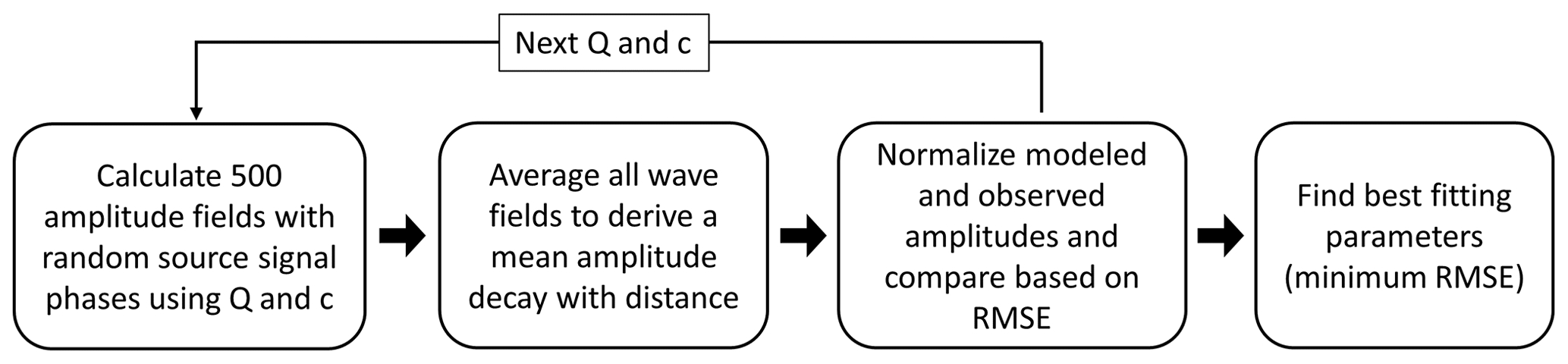
Figure 9Description of the fitting process to find the best model parameters from the comparison of calculated and observed amplitudes.
Moreover, the normalized root-mean-square error (NRMSE) is obtained to quantify the fitting quality. To determine the NRMSE, each RMSE is divided by the range (maximum value − minimum value) of the observation amplitudes for each frequency in order to scale the comparison between the datasets. The total NRMSE is then given by the mean of all normalized RMSE:
To fit modeled and observed amplitudes we performed a separate grid-search for both the group with high-frequency signals and with low-frequency signals. During each individual fitting process, the PSE method was applied to ensure results that are independent of source signals phases. Regarding the group of low-frequency signals (<4 Hz), we obtain QS=40 and cS=960 m s−1 (Table 2) as the best model parameters. The values of the 20 best models range between 36 and 60 for QS and 920 m s−1 and 1040 m s−1 for cS. Regarding the group of high-frequency signals (>4 Hz), we obtain QS=16 and cS=540 m s−1 as the best parameters. Results of the 20 best models range between 12 and 32 for QS and between 540 and 660 m s−1 for cS (Fig. 10). By fitting two frequency groups, we can derive a two-layer model (one layer with a half-space below), after converting the frequency-dependent wavelength to the corresponding penetration depth (Eq. 5). Thus, we expect a shear wave velocity of 540 m s−1 down to 37 m depth and 960 m s−1 until 280 m depth (Fig. 11). However, transition between the two layers (37 m to 91 m) is not clearly defined due to missing information for frequencies between 3.5 and 4.85 Hz. Furthermore, we can only gain information about the attenuation of signals down to a frequency of 1.14 Hz. Hence, we are limited concerning the conversion of wavelength to depth information, and we can only derive values (cS and QS) to a estimated depth of about 280 m. We cannot give information about the properties of deeper layers. The velocity error is approximated by the range of the 20 best models (Fig. 10). During the fitting process, we noticed that it was not possible to fit all seven amplitude decays with only one cS–QS model successfully, especially regarding signals with frequencies >4 Hz. A homogeneous model is consequently not reasonable in this case. However, the corresponding results are given in the Supplement (Fig. S2). Modeled and observed data are generally in very good agreement for each of the seven analyzed frequencies (Figs. 12 and 13). The very slow decrease of observed amplitudes, especially at 1.14 Hz (Fig. 12a), and the relatively strong decrease of signals with 7.6 Hz (Fig. 13c) are simulated correctly and confirm a higher attenuation with higher frequencies, as expected. For a frequency of 1.14 Hz, between x=2000 and 4000 m, modeled amplitudes are underestimated in comparison to the observations. Minor deviations between modeled and observed data for frequencies >4 Hz might be explained by local effects that are not represented in our laterally homogeneous models. Interestingly, a local increase of amplitude with distance is observable in the real data, especially for the 3.5 and 4.85 Hz signals, as well as in the simulated data (Figs. 12d and 13a). This undulation is likely caused by superimposed wave fields of multiple WTs, as indicated by the modeled radiation pattern. Moreover, the sensitivity concerning the source signal phase compositions decreases clearly with increasing frequency, which indicates that effects of phase differences between source signals are more significant for lower frequencies. The radiation patterns off the profile are quite symmetrical since the WTs are positioned in a clear geometry (in a line with similar distances between the WTs). This might not be given if the WTs are arranged in more complex layouts that could lead to locally increased or decreased amplitudes due to wave field interferences.
Table 2Best model parameters (cS and QS) to fit observed and calculated amplitude decays of low- and high-frequency signals. Depth d is estimated by assuming a surface wave penetration depth of .
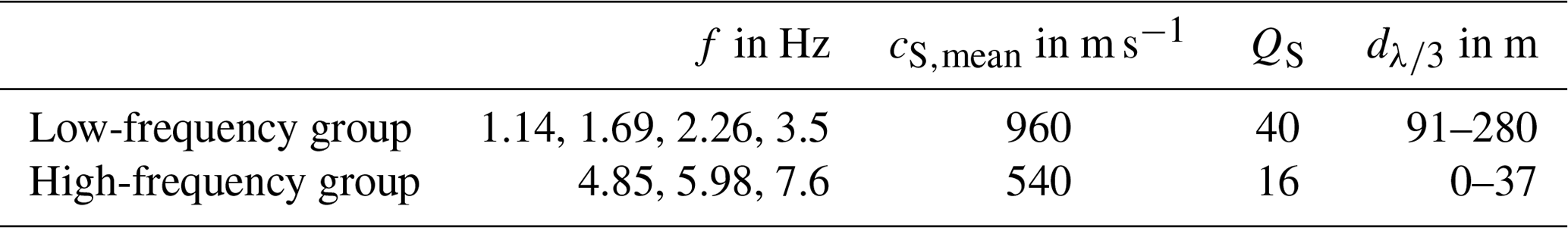
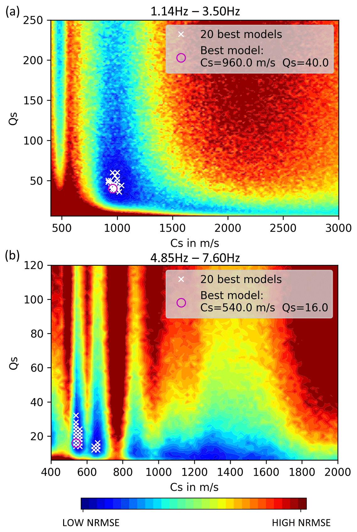
Figure 10Distribution of the NRMSE of the fit between modeled and observed amplitude decays obtained by a QS–cS grid search. The 20 best models (white cross) and the very best model (magenta circle) that fit amplitude decays of signals with (a) 1.14, 1.69, 2.26, and 3.50 Hz and (b) 4.85, 5.98 and 7.60 Hz.
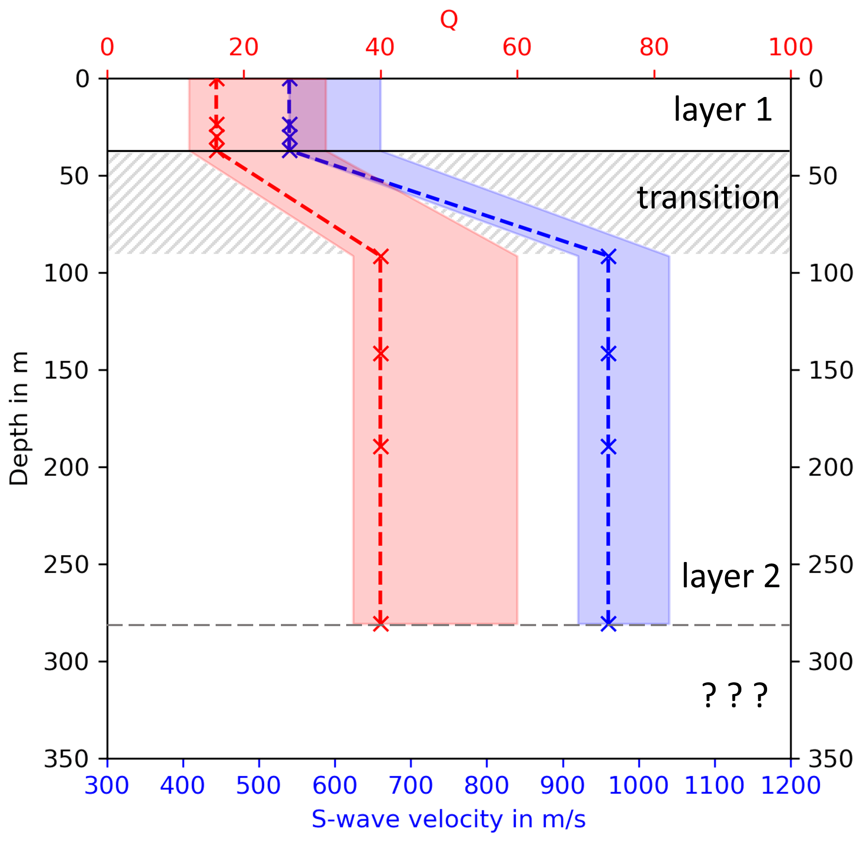
Figure 11Two-layer model derived by fitting observed and modeled amplitude decays. The best model parameters (cS and QS) for the two layers are found by performing a grid search to optimize the fitting of amplitude decays of signals <4 and >4 Hz separately. The depths of the layer interfaces are obtained by assuming a penetration depth of surface waves of . The transition between layer 1 and layer 2 and the area below layer 2 is unclear, due to the lack of amplitude decays of signals between 3.5 and 4.85 Hz and below 1.14 Hz.
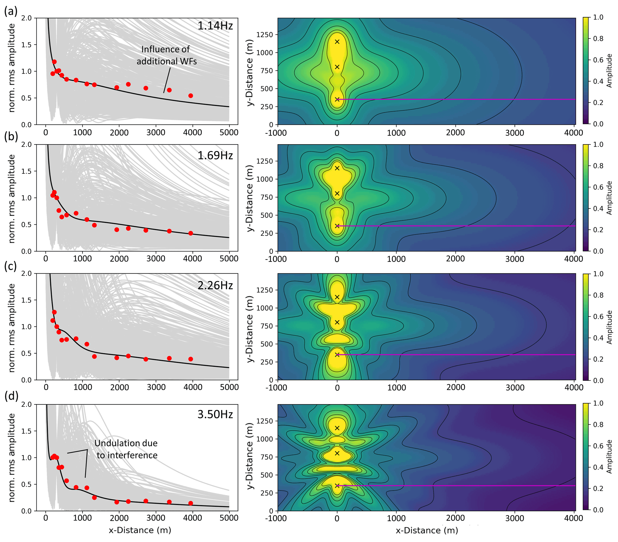
Figure 12Averaged modeled radiation patterns (right) and averaged amplitude decays (left, black line) along the profile (magenta line) by averaging 500 wave fields and decay curves (gray lines), based on random ϕ (between 0,π) to eliminate the effect of phase differences between source signals. Red dots represent the observed amplitudes in Uettingen at (a) 1.14 Hz, (b) 1.69 Hz, (c) 2.26 Hz, and (d) 3.50 Hz.

Figure 13Averaged modeled radiation patterns (right) and averaged amplitude decays (left, black line) along the profile (magenta line) found by averaging 500 wave fields and decay curves (gray lines) based on random ϕ (between 0, π) to eliminate the effect of phase differences between source signals. Red dots represent the observed amplitudes in Uettingen at (a) 4.85 Hz, (b) 5.98 Hz, and (c) 7.60 Hz.
The aim of this study is to present reliable amplitude decays of seismological signals produced by multiple WTs and to model these amplitude decays with an analytical approach. The propagation of WT-induced seismic signals has been the subject of numerous studies. Many authors found that the amplitude decay with increasing distance (r) between WT and observation point can be described by a power law of the form . In general, the absorption factor, b, increases with increasing frequency. Results found in our study show a near-perfect linear increase of the b value with frequency and range from b=0.39 at 1.14 Hz up to b=3.93 at 7.6 Hz. By converting the b values from the spectral domain (PSD) into the time domain (Table 1), we find b values <0.5 at frequencies ≤2.3 Hz, which is lower than the theoretical value for geometrical spreading of a single source surface wave. An explanation for this is the interference of the three wave fields from the three WTs. Although the decay of signals from a single WT would likely not be lower than the geometrical spreading attenuation, we can show that the superposition of wave fields could significantly increase the amplitudes along the profile. The b factors derived by the various authors cover a broad range of values, even for similar frequency ranges. Flores Estrella et al. (2017) published b values from 0.73 to 1.87 for frequencies between 2.7 and 4.5 Hz. Zieger and Ritter (2018) derived values from 0.78 to 0.85 at 1–4 Hz and b=1.59 at 5.5 Hz. The results from Lerbs et al. (2020) range between 0.7 and 1.3 at 1–4 Hz and b=2.3 at 5 Hz. Neuffer et al. (2019) derive b values of 2.4 at 3 Hz and values of b>5 at frequencies of 6–7 Hz. In Fig. 5, we compare our results with the b values of Neuffer et al. (2019) and Lerbs et al. (2020). These studies yield a similar frequency dependence. However, the results of Neuffer et al. (2019) show systematically higher b values. This observation could be due to different geological conditions with stronger attenuation effects during wave propagation. Furthermore, Neuffer et al. (2019) used so-called “differential” PSD spectra to measure the peak amplitude decay. These amplitudes are calculated from the difference between the PSD peaks at full power and the PSD peaks at zero power, which could lead to an overestimation of the amplitude decay. Lerbs et al. (2020) get similar b values; however, compared to our results the scatter is significantly larger. Most authors explain the observed b-value scattering using different local geological conditions that influence the attenuation of the emitted seismic WT signals. It should be noted, however, that some of the above-mentioned studies use relatively short time windows to estimate the spectral amplitudes at increasing distances. Flores Estrella et al. (2017) analyze time series of 2 h lengths, and Lerbs et al. (2020) use 6 h. In this case the measured amplitudes could be affected by transient signals such as earthquakes or local anthropogenic noise sources, which may result in uncertain b-value estimates. In contrast, Neuffer et al. (2019) extend the analysis to 6.5 weeks. Since the knowledge of the amplitude decay plays a fundamental role in the modeling of the WT signals, we decided to use significantly longer time windows (6 months) in order to derive robust average PSD spectra at the installed profile stations.
In terms of modeling approaches, most of the recent publications focus on modeling the seismic signals that are emitted by one single WT (e.g., Gortsas et al., 2017) or the whole WF is considered as one emitting source. Since we observe time-varying phase differences between the signals that are measured directly at the three individual WTs of the WF Uettingen, we propose that this effect must be included in the modeling of WFs. Our observations confirm the significance of phase differences between the seismic signals from the WTs of a wind farm and that the signal phase of a single WT is not stable over time. Hence, we expect that phase differences between source signals vary randomly, which was already presumed by Saccorotti et al. (2011). Superimposed wave fields lead to constructive and destructive interferences (which depend on, e.g., signal phases) and affect the spatial amplitude decay, as we can show in this study (Fig. 8). Similar to our approach, Saccorotti et al. (2011) modeled amplitude decays on the basis of superimposed wave fields and attenuation laws but did not include phase shift variations between signals of the WTs. However, they noticed that the increase of noise depends on WT number, which was later shown by Neuffer et al. (2019). Saccorotti et al. (2011) suggest that more accurate results can be derived by considering WTs that are not vibrating in phase. Here, we can prove the randomness of these phase differences between WTs and propose a solution by applying the PSE method to the modeling. Only with this consideration we can reproduce the observed amplitude decay. The PSE-method (averaging 500 wave fields calculated with random signal phases) is generally difficult to apply if full wave form propagation simulation is needed (e.g., FEM, finite element methods), since the required computation time would increase rapidly. Within our modeling approach, the source amplitude is chosen to be uniform for the three WTs. Previous studies (e.g., Lerbs et al., 2020) showed that WTs emit signals with time-varying amplitude and azimuths. In terms of modeling radiation patterns for very short time periods, this should be considered when choosing representative source characteristics. To model radiation patterns that represent long time periods (quasi-static processes), a uniform source amplitude should be sufficient, provided that the WTs are of the same type.
For the Uettingen WF the discrepancy between observed and simulated amplitude decays for 1.14 Hz in distances larger than 2000 m to the WTs are likely due to the other nearby WFs A and B (Fig. 1). We assume that the low-frequency signals of these WFs travel farther compared to higher-frequency signals and are measured in addition to the signals from the targeted three WTs in Uettingen (Fig. 1). This could lead to an overestimation of the signal amplitudes, especially in the far field of the WF Uettingen. However, since we observe peaks at identical frequencies in the near and far field of the WF, it is reasonable to assign these signals mainly to the wave field produced by the WTs in Uettingen. Signals from various WFs can generally be distinguished using, e.g., a migration approach (Friedrich et al., 2018). However, detailed analysis of the effect of additional WFs around Uettingen is beyond the scope of this study, but their impact should be considered in future analysis. Interestingly, the sensitivity to source signal phases (gray lines in Figs. 12 and 13) is significantly higher for 1.14 Hz signals than 7.6 Hz and is generally decreasing with increasing frequency. This indicates that the signal phases are not as important for higher frequencies than for lower frequencies (e.g., 1.14 Hz). It should be noted that some of the individual input source signal phase compositions led to decay curves that could not fit the observation data at all. This is solved using the PSE method.
Lerbs et al. (2020) proposed a solution that describes the wave attenuation with distance using an attenuation model solely based on a power law assumption (b values). This approach does not allow a more universal application to other WFs or regions since b values are not directly assigned to geological properties. The approach used in our study includes the intrinsic attenuation factor, which depends on two geological parameters, the seismic wave velocity and quality factor. We find frequency-dependent Q values of 16 and 40 and cS of 540 and 960 m s−1. The local geology is dominated by sedimentary rocks of the Buntsandstein, which could explain the relatively low Q values (high damping). The attenuation is very likely dominated by intrinsic attenuation and not scattering, since the topography around Uettingen is relatively smooth and large damaging zones or faults are missing. A homogeneous half-space is therefore the basic assumption within our model. However, we show that the effect of layered media in the underground should be considered assuming frequency-dependent velocity and quality factors, due to significant dispersion effects of surface waves. It is generally an advantage to include geological properties in the model: (1) to consider actual physical properties of the medium the waves are traveling through and (2) to enable the possibilities of studying the effect of various geological conditions on the seismic radiation and amplitude decays.
To demonstrate the capability and possible application of the modeling approach used in this study, we modeled the radiation pattern of the original WF in Uettingen for 1.14 and 7.6 Hz signals and compared the results with the case where three imaginary WTs are arbitrarily added to the existing WF (Fig. 14). Model parameters are cS=960 m s−1 and QS=40 for 1.14 Hz and cS=540 m s−1 and QS=16 for 7.6 Hz. The pattern of the radiation for 1.14 Hz signals is clearly affected by adding three WTs to the WF in Uettingen, whereby amplitudes are significantly increased, even in remote areas, for example in the NNW of the WF (Fig. 14a and c). The effect on the characteristic radiation of 7.6 Hz signals is negligible since the signal amplitude is damped rapidly in both cases, i.e., modeling three WTs or six WTs (Fig. 14b and d). As the demonstration shows, the modeling approach allows the estimation of the characteristic seismic radiation pattern of an arbitrary WF in order to identify locations of low or high noise amplitudes or to evaluate WF geometry effects. Furthermore, the source locations, source signal frequencies and amplitudes, and the expected local underground are free for researchers to choose (with limitations regarding their complexity), which enables an approximation of the surface wave field emitted by WFs with various layouts.
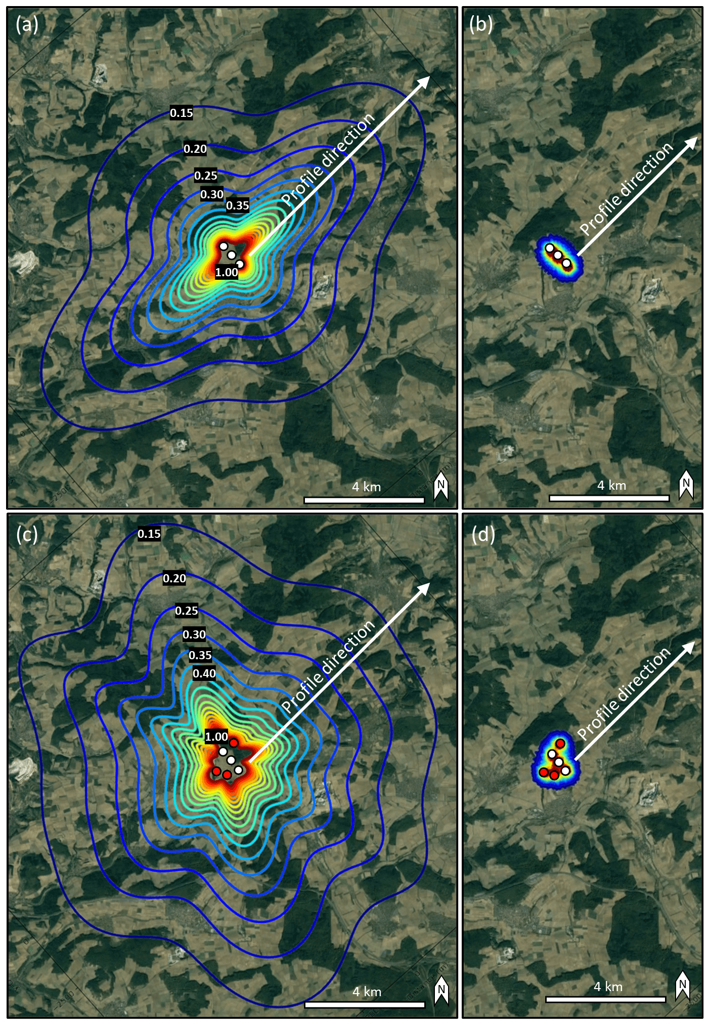
Figure 14Estimated seismic radiation pattern (red showing high amplitudes) of (a) the Uettingen wind farm (white dots) for 1.14 Hz and (b) 7.6 Hz. Three arbitrary WTs (red dots) are added to the existing WF and affect the radiation for (c) 1.14 Hz and (d) 7.6 Hz. Model parameters are cS=960 m s−1 and QS=40 in (a, c), whereas they are cS=540 m s−1 and QS=16 in (b, d). Calculations are based on 500 averaged wave fields using random source signal phases. Contour lines show the amplitude decay factor from 1 to 0.15 (map data: © Google Maps, 2021).
We recorded the seismic signals emitted from a three-turbine WF in Uettingen, Bavaria, over a period of 6 months and analyzed the spectral characteristics and spatial amplitude decays. During the full power operation mode of the WTs we identify seven prominent spectral peaks in the frequency range from 1.14 to 7.6 Hz. The attenuation of the peak amplitudes with respect to the WT distances can be described by a power law with exponent b. We find that the calculated b values increase linearly with increasing peak frequency and range between 0.39 and 3.93. Due to the relatively long observation period, the calculated values provide a stable basis for the analytical simulation of the emitted wave field.
An analytical approach was developed to model the seismic radiation of the WF. From measurements we observe that WTs are not vibrating in phase and that the phase differences vary randomly over time. Furthermore, the results of the simulation show a strong influence of phase differences between single WT source signals on the radiation pattern and hence on the spatial amplitude decays. We applied a phase shift elimination method (PSE method) to eliminate this effect with the aim of deriving a representative seismic wave field. Modeling results were compared to the observed frequency-dependent amplitude decays to derive model parameters (QS and cS) for a two-layer model that provides information about the local geology. Concerning the modeling of WT-induced seismic signals, we can show that the signal phases of multiple source signals (multiple WTs) have significant influence on the seismic radiation of the WFs. This effect should be carefully considered when selecting suitable source signals to avoid misleading simulation results.
The code and data used in this research are currently restricted.
The supplement related to this article is available online at: https://doi.org/10.5194/se-12-1851-2021-supplement.
FL and ML performed the field work and data analysis. FL set up the modeling approach and performed model calculations. GR participated in data interpretation and model development and supervised the article outline. HD and GR initiated the project and provided the computational framework. FL, ML, GR, and HD edited the article.
The authors declare that they have no conflict of interest.
Publisher’s note: Copernicus Publications remains neutral with regard to jurisdictional claims in published maps and institutional affiliations.
We would like to thank ESWE Versorgungs AG for providing access to the wind farm facilities in Uettingen and their operational data, and we would especially like to thank Ulrich Schneider for his support in initiating the project. We appreciate the support of the mayors of Uettingen, Greußenheim, Remlingen, and Leinach as well as their respective municipal administrations. Special thanks are given to Wolfgang Reinhart, Joachim Palm, and Ana Costa for their help during fieldwork and station maintenance and to Gabriele Schmidt (ESWE), who was our contact person regarding technical matters of the WF Uettingen.
This research is part of the project KWISS and has been supported by the German Federal Ministry for Economic Affairs and Energy (FKZ no. 0324360) and ESWE Innovations und Klimaschutzfonds.
This open-access publication was funded by the Goethe University Frankfurt.
This paper was edited by Charlotte Krawczyk and reviewed by Joachim Ritter and Hortencia Flores Estrella.
Bugeja, R.: Crustal Attenuation in the region of the Maltese Islands using CodaWave Decay, PhD thesis, Department of Physics, University of Malta, 2011.
Bayerisches Geologisches Landesamt: Geologische Karte von Bayern 1:25.000, Blatt 6124, Remlingen, München, 1978.
Farrugia, D., Paolucci, E., D'Amico, S., Galea, P., Pace, S., Panzera, F., and Lombardo, G.: Evaluation of seismic site response in the Maltese archipelago, in: Establishment of an Integrated Italy–Malta Cross–Border System of Civil Protection, Geophysical Aspects, 79–98, Chapter: V, 2015.
Flores Estrella, H., Korn, M., and Alberts, K.: Analysis of the Influence of Wind Turbine Noise on Seismic Recordings at Two Wind Parks in Germany, Journal of Geoscience and Environment Protection, 5, 76–91, https://doi.org/10.4236/gep.2017.55006, 2017.
Friedrich, T., Zieger, T., Forbriger, T., and Ritter, J. R. R.: Locating wind farms by seismic interferometry and migration, J. Seismol., 22, 1469–1483, https://doi.org/10.1007/s10950-018-9779-0, 2018.
Gortsas, T. V., Triantafyllidis, T., Chrisopoulos, S., and Polyzos, D.: Numerical modelling of micro-seismic and infrasound noise radiated by a wind turbine, Soil Dyn. Earthq. Eng., 99, 108–123, https://doi.org/10.1016/j.soildyn.2017.05.001, 2017.
Hayashi, K.: Development of the Surface-wave Methods and Its Application to Site Investigations, PhD thesis, Kyoto University, Japan, 2008.
Karatzetzou, A., Negulescu, C., Manakou, M., François, B., Seyedi, D. M., Pitilakis, D., and Pitilakis, K.: Ambient vibration measurements on monuments in theMedieval City of Rhodes, Greece, B. Earthq. Eng., 13, 331–345, https://doi.org/10.1007/s10518-014-9649-2, 2014.
Kumagai, T., Yanagibashi, T., Tsutsumi, A., Konishi, C., and Ueno, K.: Efficient surface wave method for investigation of the seabed, Soils Found., 60, 648–667, https://doi.org/10.1016/j.sandf.2020.04.005, 2020.
Larose, E.: Lunar subsurface investigated from correlation of seismic noise, Geophys. Res. Lett., 32, L16201, https://doi.org/10.1029/2005gl023518, 2005.
Leiber, C.-O.: Assessment of safety and risk with a microscopic model of detonation, Elsevier, Amsterdam Boston, ISBN 0444513329, 2003.
Lerbs, N., Zieger, T., Ritter, J., and Korn, M.: Wind turbine induced seismic signals: the large-scale SMARTIE1 experiment and a concept to define protection radii for recording stations, Near Surf. Geophys., 18, 467–482, https://doi.org/10.1002/nsg.12109, 2020.
Neuffer, T. and Kremers, S.: How wind turbines affect the performance of seismic monitoring stations and networks, Geophys. J. Int., 211, 1319–1327, https://doi.org/10.1093/gji/ggx370, 2017.
Neuffer, T., Kremers, S., and Fritschen, R.: Characterization of seismic signals induced by the operation of wind turbines in North Rhine-Westphalia (NRW), Germany, J. Seismol., 23, 1161–1177, https://doi.org/10.1007/s10950-019-09866-7, 2019.
Neuffer, T., Kremers, S., Meckbach, P., and Mistler, M.: Characterization of the seismic wave field radiated by a wind turbine, J. Seismol., 25, 825–844, https://doi.org/10.1007/s10950-021-10003-6, 2021.
Rahman, M. and Michelitsch, T.: A note on the formula for the Rayleigh wave speed, Wave Motion, 43, 272–276, https://doi.org/10.1016/j.wavemoti.2005.10.002, 2006.
Saccorotti, G., Piccinini, D., Cauchie, L., and Fiori, I.: Seismic Noise by Wind Farms: A Case Study from the Virgo Gravitational Wave Observatory, Italy, B. Seismol. Soc. Am., 101, 568–578, https://doi.org/10.1785/0120100203, 2011.
Siena, L. D., Thomas, C., Waite, G. P., Moran, S. C., and Klemme, S.: Attenuation and scattering tomography of the deep plumbing system of Mount St. Helens, J. Geophys. Res.-Sol. Ea., 119, 8223–8238, https://doi.org/10.1002/2014jb011372, 2014.
Stammler, K. and Ceranna, L.: Influence of Wind Turbines on Seismic Records of the Gräfenberg Array, Seismol. Res. Lett., 87, 1075–1081, https://doi.org/10.1785/0220160049, 2016.
Styles, P., Stimpson, I., Toon, S., England, R., and Wright, M.: Microseismic and Infrasound Monitoring of Low Frequency Noise and Vibrations from Windfarms, PhD thesis, Keele University, UK, 2005.
Welch, P.: The use of fast Fourier transform for 335 the estimation of power spectra: A method based on time averaging over short, modified periodograms, IEEE Transactions on Audio and Electroacoustics, 15, 70–73, https://doi.org/10.1109/tau.1967.1161901, 1967.
Westwood, R. F. and Styles, P.: Assessing the seismic wavefield of a wind turbine using polarization analysis, Wind Energy, 20, 1841–1850, https://doi.org/10.1002/we.2124, 2017.
Zieger, T. and Ritter, J. R. R.: Influence of wind turbines on seismic stations in the upper rhine graben, SW Germany, J. Seismol., 22, 105–122, https://doi.org/10.1007/s10950-017-9694-9, 2018.
Zieger, T., Nagel, S., Lutzmann, P., Kaufmann, I., Ritter, J., Ummenhofer, T., Knödel, P., and Fischer, P.: Simultaneous identification of wind turbine vibrations by using seismic data, elastic modeling and laser Doppler vibrometry, Wind Energy, 23, 1145–1153, https://doi.org/10.1002/we.2479, 2020.