Constraining 3D geometric gravity inversion with a 2D reflection seismic profile using a generalized level set approach: application to the eastern Yilgarn Craton

One of the main tasks in 3D geological modeling is the boundary parametrization of the subsurface from geological observations and geophysical inversions. Several approaches have been developed for geometric inversion and joint inversion of geophysical datasets. However, the robust, quantitative integration of models and datasets with different spatial coverage, resolution, and levels of sparsity remains challenging. One promising approach for recovering the boundary of the geological units is the utilization of a level set inversion method with potential field data. We focus on constraining 3D geometric gravity inversion with sparse lower-uncertainty information from a 2D seismic section.

We use a level set approach to recover the geometry of geological bodies using two synthetic examples and data from the geologically complex Yamarna Terrane (Yilgarn Craton, Western Australia). In this study, a 2D seismic section has been used for constraining the location of rock unit boundaries being solved during the 3D gravity geometric inversion. The proposed work is the first we know of that automates the process of adding spatially distributed constraints to the 3D level set inversion. In many hard-rock geoscientific investigations, seismic data are sparse, and our results indicate that unit boundaries from gravity inversion can be much better constrained with seismic information even though they are sparsely distributed within the model. Thus, we conclude that it has the potential to bring the state of the art a step further towards building a 3D geological model incorporating several sources of information in similar regions of investigation.

1 Introduction

Inverted models from geophysical inversions have broad applications in 3D geological modeling if they specify distinct rock units rather than just petrophysical distributions. One way to achieve this is by using geometric inversion approaches. These methods are receiving increasing attention in geophysical inverse problems with a focus on recovering the shape of different rock units. Using several geophysical techniques that enable us to recover the geometry of the specified rock type leads to an inverted model consistent with geophysical datasets that is compatible with geological interpretations.

Gravity datasets are some of the most widely modeled geophysical datasets worldwide. The inversion of gravity datasets can either be performed with the aim of retrieving density contrasts (Boulanger and Chouteau, 2001; Lamichhane and Gross, 2017; Li and Oldenburg, 1998; Martin et al., 2020; Ogarko et al., 2021) or depth and shapes (geometry) of unit boundaries (Cai and Zhdanov, 2015; Li et al., 2016). Geometric inversion approaches generate models with distinct density contrast units suitable for geological modeling purposes (Jessell et al., 2014; Leliévre et al., 2015; Lindsay et al., 2013). As complementary information is required to compensate for poor vertical resolution of gravity datasets (Coutant et al., 2012; Lelièvre et al., 2010; Sun and Li, 2015), the geometry of the retrieved models from geometric gravity inversions are more plausible if the models are compensated in depth with other geophysical datasets.

On the other hand, seismic images provide a higher vertical resolution of deep structures, and the detectable horizons from these images can be correlated with the density contrast surfaces. This enables us to utilize seismic information from the subsurface structures to constrain the gravity inversion. Combining these interpretations with a geometric gravity inversion is a step toward a geologically plausible gravity inversion in agreement with seismic images.

The level set approach being widely applied in geometry optimization problems (Osher et al., 2004) can be applied to geophysical inversion techniques by parametrizing the rock unit boundaries implicitly as iso-contours of higher dimensional functions (Li et al., 2016). Boundaries are then optimized during the inversion by evolving these level set functions (Burger and Osher, 2005). The defined units in the model can then be merged and separated or even omitted during the inversion based on topological rules (Cai and Zhdanov, 2015; van Zon and Roy Chowdhury, 2010).

Recovering rock unit boundaries using a level set gravity inversion method has been studied in recent years with the focus on inversion for different numbers and shapes of the buried bodies (Cai and Zhdanov, 2017; Farquharson et al., 2008; Leliévre et al., 2015; Li et al., 2016; Zheglova et al., 2018). However, automatic geologically conditioned geophysical level set inversion has not been addressed in the aforementioned studies. This is because the proposed methods are either limited to a specific number of units (level set functions) or are bound to a specific type of topology by using explicit modeling for defining rock units.

We utilize a generalized level set inversion technique introduced by Giraud et al. (2021a). This approach extends level set methods previously developed by Cardiff and Kitanidis (2009) and Li et al. (2017). This generalized level set algorithm, which uses a least-squares framework, allows us not only to define an arbitrary number of density contrast units free of shape limitation but also to add sparsely distributed low-uncertainty data to constrain the gravity inversion. We use information from the seismic section as low-uncertainty data because in large-scale studies borehole data might not necessarily be available for constraining purposes (for more details about the methodology, we refer readers to the following sources: Li et al., 2017; Raponi et al., 2017; Tai and Chan, 2004; Giraud et al., 2021a).

In this study, we focus on constraining surface gravity data that possess good lateral resolution with a 2D reflection seismic profile that traverses the study area. In this manner, sparsely distributed low-uncertainty data from the seismic section can be utilized to guide 3D gravity inversion results. The proposed work is the first we know of that quantitatively integrates the geometries from the seismic section into 3D gravity inversion. Our results suggest that the proposed approach has the potential to bring the state of the art a step further towards automatically building a 3D geological model that is consistent with available geological and geophysical datasets.

The remainder of this paper is organized as follows. We first provide a summary of the generalized level set method we use and show its applicability to gravity inversion constrained by sparser seismic data and geological knowledge. We then apply the proposed approach on two 3D synthetic datasets to show the proof-of-concept. Subsequently, we present a case study at the geologically complex Yamarna Terrane in Yilgarn Craton, Western Australia. We use the 3D surface gravity datasets and a 2D seismic profile available in this area to apply the constrained inversion approach. Finally, the performance of the constrained level set approach on the synthetic and field studies and the resulting models are reviewed and assessed in the discussion section.

2 Method

2.1 Generalized level set method

We use the generalized level set inversion formulation introduced by Giraud et al. (2021a) for our constrained inversion problem. We extend their work to the use of sparse seismic constraints and topological rules. A summary of the method is provided below. We only repeat essential information about this approach in this section, with the corresponding equations provided in Appendix A. For more details about the mechanics of the inverse problem we refer the readers to Giraud et al. (2021a).

In the generalized level set approach, as illustrated in Fig. 1, the model is discretized by cubic cells. Each model cell is defined by a density contrast corresponding to a given rock unit. The interfaces between rock units are defined on the same mesh where changes from one density contrast to another occur. In this inversion framework, physical properties are kept constant within the rock units and the location of interfaces between different units are allowed to change during the inversion to reduce the data misfit. To illustrate the approach we have created Fig. 1. In the conceptual 3D model of Fig. 1a, a geologically plausible model is defined with density contrasts $\mathrm{\Delta }{\mathit{\rho }}_{k=\mathrm{1},\mathrm{\dots },N}$ assigned to each of the N rock units. Then for each unit, signed-distance values to interfaces (ϕ_k) are calculated using the fast-marching method (Sethian, 1999), where the boundary of a given unit is defined by ϕ_k=0. For example, in Fig. 1a we have shown the calculated signed distances along an extracted 1D model for the rock unit 1.

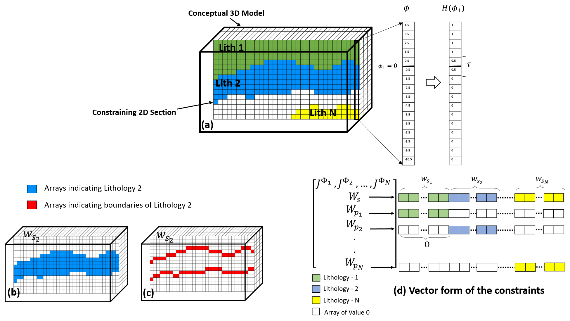
Figure 1 Illustration of the process of appending constraints to the level set problem from a sample 2D section. Panel (a) shows discretization of a conceptual 3D model and the constraining 2D section within the model that comprises N rock units; a 1D sample is extracted along the section to illustrate the calculation of signed distance and the corresponding smeared-out Heaviside function. The boundary in this case is as thick as the dimension of two cells. (b) Distribution of the constraining matrix for the entire rock unit 2 and (c) for the corresponding boundaries. Panel (d) shows the transformation of the constraints to vector forms defining the sensitivity matrix.

A smeared-out Heaviside function as introduced in Eq. (A2) is then defined that allows identifying the interfaces between rock units. This has also been exemplified in the extracted 1D model after calculating the signed distances in Fig. 1a. After defining signed distance and Heaviside values, physical-property models (m, with M number of cells) are generated for each rock unit following Eq. (A3). During inversion, the evolution of the model between two successive iterations can be controlled by a thickness parameter (τ). It can be dependent on the cell size or chosen arbitrarily. τ is an important parameter controlling the search space in the vicinity of the interface in each model update.

Defining the model as a function of signed-distance values requires the definition of a new sensitivity matrix (J^ϕ). This sensitivity matrix is then used in a least-squares inversion formulation as in Eq. (1). In this framework, residuals $\left(\mathit{r}={\left[{\mathit{d}}^{\mathrm{obs}}-{\mathit{d}}^{\mathrm{calc}}\right]}^{\mathrm{T}}\right)$ of the calculated (d^calc) and observed (d^obs) datasets are minimized during the inversion. The iterative scheme of this approach comes from a linearization of the problem around the current model. The system of equations is then dumped into a least-squares system of equations that are solved using the least-square algorithm (Paige and Saunders, 1982). The data misfit term to minimize can be written as follows:

$$\begin{array}{}\text{(1)}& {\mathbf{\Psi }}^r={∥\left({\mathit{d}}^{\mathrm{obs}}-{\mathit{d}}^{\mathrm{calc}}\right)-{\mathbf{J}}^{\mathit{\varphi }}\mathit{\delta }\mathit{\varphi }∥}_{\mathrm{2}}^{\mathrm{2}}.\end{array}$$

Here Ψ^r represents the misfit function.

The misfit function is minimized iteratively to solve for changes in the signed-distance function (δϕ_k). For details about the mathematical notations for the introduced steps above, we refer the readers to Appendix A, where the essential material from Giraud et al. (2021a) is presented. To stabilize the inversion problem and incorporate prior information, regularization terms are added to Eq. (1) as discussed below. We use an updated form of the regularizations as spatial constraints to the inversion problem based on seismic information using the aforementioned method. To encourage geological plausibility, we then introduce the utilization of topological rules on the resulting model during inversion. The utilization of seismic information to define regularizations is introduced below.

2.2 Regularized level set inversion

Other level set inversion approaches (Li et al., 2016, 2017; Zheglova et al., 2018) apply regularizations to the misfit function. In such cases, the problem is usually regularized by favoring structures with the shortest interface overall length (2D case) or smallest surface (3D case). Minimizing the length of the geometries generates shapes with the smallest area, and regularizing these inversion problems can be limited to the specific shape of units that can introduce a bias towards unrealistically simple geometries. Using known density contrast values for the model parameterization in these approaches significantly reduces the non-uniqueness of the inversion. In addition, regularizing the inverted model using prior information may reduce the non-uniqueness of the inverse problem further. In the level set inversion scheme we use, prior information can be appended as regularization terms (Ψ^t) in the same fashion as smallness terms regularize inversion problems (Calvetti et al., 2000). This term is appended to the misfit function as follows:

$$\begin{array}{}\text{(2)}& \mathbf{\Psi }\left(\mathit{\delta }\mathit{\varphi },\mathit{r}\right)={\mathbf{\Psi }}^r\left(\mathit{\delta }\mathit{\varphi },\mathit{r}\right)+{\mathbf{\Psi }}^t\left(\mathit{\delta }\mathit{\varphi }\right),\end{array}$$

where

$$\begin{array}{}\text{(3)}& {\mathbf{\Psi }}^t\left(\mathit{\delta }\mathit{\varphi }\right)={∥\begin{array}{l}{\mathit{W}}_{\mathrm{S}}\mathit{\delta }\mathit{\varphi }\\ {\mathit{W}}_{\mathrm{P}}\mathit{\delta }\mathit{\varphi }-\mathit{V}\end{array}∥}_{\mathrm{2}}^{\mathrm{2}}.\end{array}$$

Here W_S is a global regularization 1×MN vector and W_P is a local regularization N×MN matrix that has ${\mathit{W}}_{p_{k=\mathrm{1},\mathrm{2},\mathrm{\dots }N}}$ as rows. Both W_S and W_P encapsulate prior information for the inversion. In general, Ψ^t tends to minimize the total update in the signed distance (δϕ) and acts as a smallness term that encourages the product (Wδϕ) of rock units to reach specific values stored in $\mathit{V}=\left({\mathit{v}}_{\mathrm{1}},{\mathit{v}}_{\mathrm{2}},\mathrm{\dots },{\mathit{v}}_N\right)$.

Inverting for the total changes in the signed-distance value at each model update and controlling these changes through regularizations enables us to extend the approach for the constrained inversion problems. In the next subsection, we introduce the method we developed to incorporate 2D information into the regularization scheme presented here using the case of 2D seismic data. We show that by updating global and local regularization terms with low-uncertainty information from seismic datasets, regularization terms can act as constraints.

2.3 Translating seismic information to spatial constraints

Global (W_S) and local (${\mathit{W}}_{p_{k=\mathrm{1},\mathrm{\dots },N}})$ regularization terms are appended to the sensitivity matrix of the level set method as in Eq. (4) as vectors in a system of equations solved in the least-squares sense. They tend to stabilize changes of signed-distance functions as damping terms. This supports the capability of regularization terms to perform the constraining process using low-uncertainty datasets such as seismic data as weighing terms. We use the global regularization term to encapsulate the information about all rock units in one vector while local terms are defined to include different rock units separately in the inversion problem. The different effects of these two terms are also reflected in Eq. (4). We propose that adding unevenly distributed weights to the regularizations based on information from seismic data in depth can act as constraints for the level set inversion. Therefore, as long as the interpreted or inverted sections from the seismic data are included in vectors with the same size as the model, any primary information from pre-existing modeling such as seismic sections can be translated to weighting terms to define constraints.

$$\begin{array}{}\text{(4)}& \left[\begin{array}{l}{\mathbf{J}}^{{\mathit{\varphi }}_{\mathrm{1}}}{\mathbf{J}}^{{\mathit{\varphi }}_{\mathrm{2}}}\mathrm{\dots }{\mathbf{J}}^{{\mathit{\varphi }}_N}\\ {\mathit{W}}_{\mathrm{S}}\\ {\mathit{W}}_{p_{\mathrm{1}}}\\ {\mathit{W}}_{p_{\mathrm{2}}}\\ .\\ .\\ {\mathit{W}}_{p_N}\end{array}\right]\left[\begin{array}{l}\mathit{\delta }{\mathit{\varphi }}_{\mathrm{1}}\\ \mathit{\delta }{\mathit{\varphi }}_{\mathrm{2}}\\ .\\ .\\ \mathit{\delta }{\mathit{\varphi }}_N\end{array}\right]=\left[\begin{array}{l}\mathit{r}\\ \mathrm{0}\\ v_{\mathrm{1}}\\ v_{\mathrm{2}}\\ .\\ .\\ v_N\end{array}\right]\end{array}$$

Strategies for transferring the knowledge from a seismic section to a weighting term that can be used as sparse constraints can vary depending on the seismic data and availability of other datasets. Overall, the interpretation from a vertically extended seismic profile can be assumed as an interpreted sample geological model. In Fig. 1a, we assume that within a 3D conceptual model, interpretations are available in 2D that have led to a conceptual geological model comprising of N rock units (shown as constraining 2D section). Therefore, 2D seismic interpretations are treated in the same fashion as a 2D geological surface map to constrain the gravity inversion at depth. Constructing the weighted regularization terms or constraint terms based on available interpretation is necessary before starting the inversion, which is also illustrated in Fig. 1. All parts of the 3D model that lie within the constraining section are weighted accordingly for all rock units as ${\mathit{w}}_{s_{k=\mathrm{1},\mathrm{\dots },N}}$ (all of dimensions 1×M), which then construct the regularization terms as in Eq. (5). Thus, the values of W_S and ${\mathit{W}}_{p_{k=\mathrm{1},\mathrm{\dots },N}}$ are adjusted locally according to seismic interpretations to favor the preservation of interpreted units along the seismic section. The structure of weighting vectors from seismic interpretations within regularization terms is as follows.

$$\begin{array}{}\text{(5)}& \left\{\begin{array}{l}{\mathit{W}}_{\mathrm{S}}=\left[{\mathit{w}}_{s_{\mathrm{1}}},{\mathit{w}}_{s_{\mathrm{2}}},\mathrm{\dots },{\mathit{w}}_{s_N}\right]\\ {\mathit{W}}_{p_{\mathrm{1}}}=\left[{\mathit{w}}_{s_{\mathrm{1}}},\mathit{O},\mathrm{\dots },\mathit{O}\right]\\ {\mathit{W}}_{p_{\mathrm{2}}}=\left[\mathit{O},{\mathit{w}}_{s_{\mathrm{2}}},\mathrm{\dots },\mathit{O}\right]\\ .\\ .\\ {\mathit{W}}_{p_N}=\left[\mathit{O},\mathit{O},\mathrm{\dots },{\mathit{w}}_{s_N}\right]\end{array}\right.\end{array}$$

Here O is a zero vector of dimensions 1×M.

Figure 1 shows the weighting matrix for a given rock unit (in this case rock unit 2) and its location within regularization terms as ${\mathit{w}}_{s_{\mathrm{2}}}$. As shown in Fig. 1b, in a 3D volume with the same size as the model, the extracted section along the seismic profile is weighted accordingly for rock unit 2. These spatially distributed weighting sections (matrices) are then transferred to vectors (Fig. 1d) and applied as global and local constraints to the previously introduced regularization terms. It is important to increase the values of weights to reduce model updates around the seismic interpretations and to suppress the changes of the interface locations in low-uncertainty areas.

As the calculation of the sensitivity matrix (J^ϕ) is limited to the vicinity of interfaces defined by τ, the search space for applying the constraints can also be limited to neighboring cells around interfaces. This indicates that regularizations can also be adjusted at boundaries between units rather than the entire rock units. This can be advantageous in cases where extracting the array locations along the boundaries is straightforward. Detected unit boundaries from other sources of information (geological and geophysical) can then be directly transferred to weighting matrices to be used in the constrained level set inversion. As a result, the constructed constraints ${\mathit{w}}_{s_{\mathrm{2}}}$ in Fig. 1b can also be represented as Fig. 1c. Boundaries' parametrization from interpretations or inversion (such as acoustic impedance inversion) of seismic data after depth conversion and projection onto the mesh used for the inversion can be directly used as regularizations. Therefore, the interpreted boundaries from regional seismic studies or from inversion are digitized as weighting matrices and used as constraints. Demonstration of the structure of a weighting matrix along boundaries of a given unit of the conceptual model can be observed in Fig. 1c.

As the application of sparse constraints enforces local restrictions to the evolution of signed-distance values, the resulting model from ensembles of signed-distance functions for different rock units also requires constraints to enforce small-scale topological rules accordingly with geological knowledge and to ensure that certain configurations do not occur during inversion. This is covered in the next subsection.

2.4 Enforcing topological rules

Topological constraints play a paramount role in geo-modeling processes (Burns, 1988; Pellerin et al., 2017; Perrin and Rainaud, 2013; Thiele et al., 2016). They refer to properties of a model that are changing during the perturbation of a model. Topological relationships can be defined over discontinuity networks (fractures or faults) (Sanderson and Nixon, 2015), rock units, or unconformities (Jessell et al., 2010) and are decisive components in the 3D modeling process. In recent years, these relationships are being considered computationally either explicitly or implicitly (Pakyuz-Charrier et al., 2018a, b) and as constraints for probabilistic 3D models (de La Varga et al., 2019) in the context of 3D geological modeling. Furthermore, in the geophysical inversion context, they have sometimes been addressed by means of uncertainty quantifications during inversion and joint-inversion problems (Giraud et al., 2019b, 2017; Wellmann et al., 2018) or as post-inversion regularization analysis (Cracknell and Reading, 2015; Giraud et al., 2020; Tarabalka et al., 2009). However, to the best of our knowledge, the application of the topological relationships while deforming discrete units in geophysical inversion problems has not been addressed.

Among the different orders of topology (Thiele et al., 2016), we focus on first-order topology describing adjacency relationships between rock units. The utilized level set inversion approach allows us to enforce small-scale topological rules as morphological constraints to the inversion problem. To ensure that inverted models remain geologically realistic, we apply topological rules at each iteration. We take advantage of a certain type of morphological rule to prevent the nucleation of a given unit into another and to ensure that the model obeys topological rules. This becomes important for retaining the integrity of the predefined unit boundaries during the inversion and ensuring the geological plausibility of the inverted model (age and deformation history).

Application of the mathematical morphology on geoscientific datasets has been evaluated based on the classification of input data types (Heijmans, 1995; Serra, 1986; Soille and Pesaresi, 2002). However, it has rarely been applied within geophysical inversion problems. Given that in a level set inversion problem the model space can be assumed as an image where the ordering of signed-distance values matters more than property values, morphological opening or closing (Vincent, 1993) rules can be applied on each of rock units (b^RU) at each iteration. For a 3D model, considering a structuring element γ of size ${\left(m\times n\times p\right)}_{\mathrm{0}<m,n,p<\mathrm{model}\mathrm{dimension}}$, the closing notation (•) of b^RU can be shown as

$$\begin{array}{}\text{(6)}& {\mathbf{b}}^{\mathrm{RU}}•\mathit{\gamma }=\left({\mathbf{b}}^{\mathrm{RU}}\ominus \mathit{\gamma }\right)\oplus \mathit{\gamma },\end{array}$$

where ⊖ and ⊕ demonstrate morphological dilation and erosion, respectively (Jankowski, 2006; De Natale and Boato, 2017). This operation ensures that all neighboring model cells with the size of a structuring element that does not fit in the background density will be closed, and thus nucleation of each rock unit with size that is greater than $\left(m\times n\times p\right)$ is prevented from occurring.

3 Synthetic examples

The aim of this section is to study the application of the introduced procedure on two synthetic case studies. We first benchmark the method using a well-known model and then simulate a more realistic application in a hard-rock scenario where 2D constraints are applied in a 3D inversion setting.

3.1 SEG/EAGE salt dome model

In this section, we use a simplified version of the SEG/EAGE salt dome model (Aminzadeh, 1996) in the same fashion as Li et al. (2016). This example demonstrates the application of the regularized level set inversion for a model of two distinct rock units. We assume the salt dome in Fig. 2a with the −470 kg m⁻³ density contrast in a void background assuming 2670 kg m⁻³ as the base density. We discretize the model to cells of 200 m. The model extends from 0 to 13 520 m in both horizontal directions and from 0 to 4000 m in depth (generating a model volume of size $n_x\times n_y\times n_z=\mathrm{68}\times \mathrm{68}\times \mathrm{21}$ = 97 104). A cross section of the model and the corresponding synthetic seismic image is extracted along the oblique line ($t-t^{\prime }$) in Fig. 2c (from X_t=3000, Y_t=0 to $X_{t^{\prime }}$ = 13 000, $Y_{t^{\prime }}$ = 11 000 m) to image the salt body for the constraining purpose. We also add 5 % noise with normal distribution to the forward-calculated gravity datasets to generate the field datasets on the surface $(N_x\times N_y=\mathrm{30}\times \mathrm{30}=\mathrm{900})$. It is assumed that the subsalt boundary and the dipping part of the salt have been poorly imaged and are not interpretable from the seismic section (Fig. 2b). This restricts the constraining matrices from the seismic section to the upper boundary of salt (Fig. 2d). The constraining matrices are then appended to the sensitivity matrix as global and local regularizations for both units.

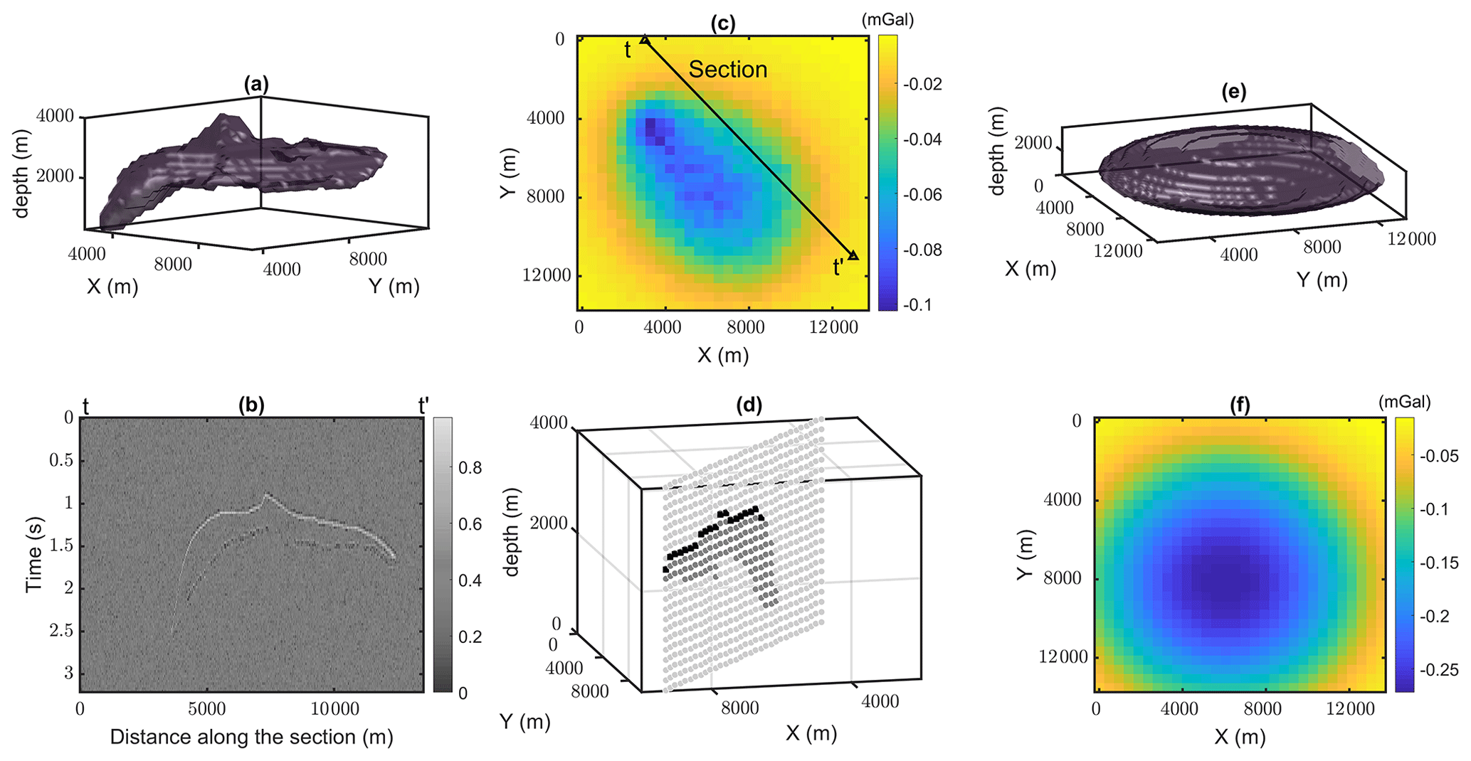
Figure 2 (a) Simplified SEG/EAGE salt model in 3D. (b) Generated synthetic seismic along section shown in (c). (c) Forward-calculated gravity data of the true model on the surface with 5 % noise. (d) Extraction of the model along the seismic line to construct the constraining matrix, the black cubes represent the location of indices of the constraining matrix with the maximum weight (400) based on the seismic image. (e) Starting model for the inversion and (f) the calculated forward gravity data of the starting model.

In many of the real-case scenarios the starting model, despite following the primary assumptions in the region, might be far from reality. Thus, we start the inversion using a simplistic starting model that is different from the true model to test and evaluate the similarity between the resulting geometry and the true geometry. In this example, we consider a disk as a starting model (Fig. 2e) that has intersections with two edges of the model boundaries.

The results of the level set gravity inversion of the salt dome using the starting model in Fig. 2e, with and without the utilization of seismic information, are illustrated in Fig. 3. The resulting model demonstrated in Fig. 3a is recovered after applying constraints along 2D seismic section based on the well-imaged upper boundary of the salt. We apply the constraints for this example along the seismic section using the weighting value (400) along the well-imaged top salt boundary (black cubes in Fig. 2d). The initialized value for τ is considered 100.2 m. The data misfit error decreases smoothly and converges to 0.8 mGal after almost four iterations. Due to the simplicity of the model, the morphological closing is not included during the inversion of this model.

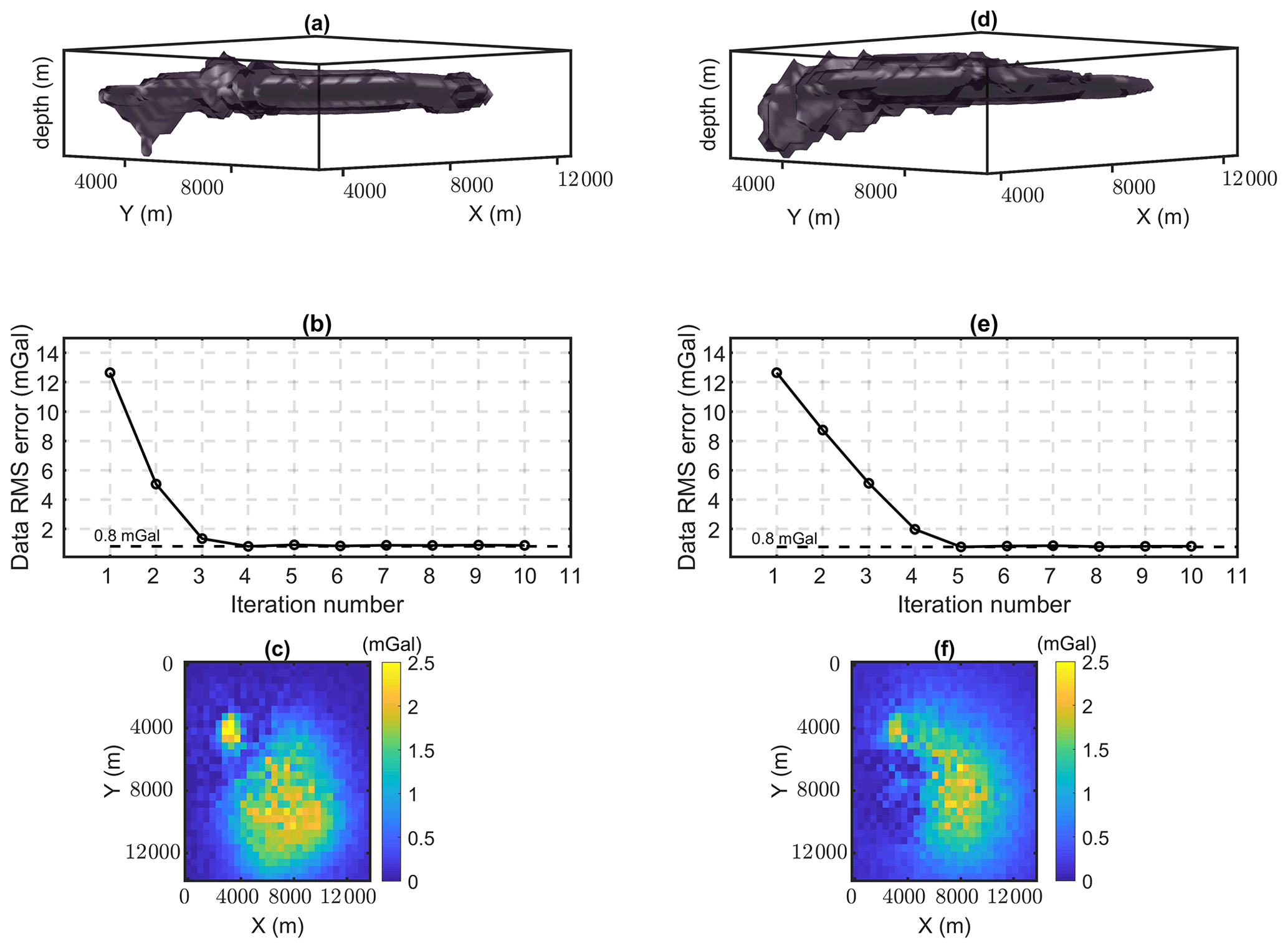
Figure 3 The 3D views of the inverted model from the constrained (a) and unconstrained inversion (d). Corresponding evolution of data root-mean-square errors (RMSEs) (b, e), and (c) the corresponding final calculated difference between the field and calculated gravity datasets (c, f).

The number of iterations toward convergence in this example is noticeably low for imaging the salt body for both the constrained and unconstrained inversion. The model misfit between the resulting inverted model from the constrained inversion and the true model (99 kg m⁻³) is slightly smaller than the model misfit resulting from the unconstrained inversion (106.2 kg m⁻³). Although the lower boundary of the salt has not been constrained by the seismic image, application of the constraints to the upper part of the salt body has also improved the imaging of the subsalt.

The application of the regularized inversion to a more complex model by utilizing regularization terms in a vertical section is provided in the next section.

3.2 Example of hard-rock synthetic case

We have also tested the method on a second generated synthetic model (Fig. 4a) that contains four distinct rock units with different density contrasts. The model simulates a hard-rock scenario and contains two exposed bodies (greenstones) with the same density contrast (330 kg m⁻³) surrounded by lower-density rock units (granitic background). This model is considered the true model, and the aim of the 3D generalized level set inversion is to recover a model that is structurally close to the true model by constraining the inversion using the seismic information available in the area. The model is composed of $n_x\times n_y\times n_z=\mathrm{40}\times \mathrm{30}\times \mathrm{40}$ = 48 000 cubic model cells with 50 m resolution. A zero-offset straight synthetic seismic section along y=750 m using a finer grid mesh (10 m each cell dimension) is generated, and 2 % random noise with normal distribution is added to the amplitudes (Fig. 4c). The true model is then used to simulate gravity anomaly data at surface level ($N_x\times N_y=\mathrm{36}\times \mathrm{26}=\mathrm{936}$) with 50 m spacing and assuming padding of 100 m. We add 5 % noise with normal distribution to the gravity measurements (Fig. 4b). As the main focus of this study is to test the application of 2D vertical constraints in a 3D level set inversion, we generate the starting model using only information from the seismic section. For the purpose of testing our algorithm, we simulate a starting model with an inaccurate representation of the geology of the area, specifically connectivity of the greenstones and differences between the position and dipping of all layers (Fig. 4d). The starting model is used to initialize the signed-distance functions. To add distributed constraints along the seismic section to the inversion, we use the absolute value of reflectivity coefficients multiplied by constant values to directly translate boundaries from the seismic section to weighting matrices in the level set formulation in Eq. (5). Translating these boundaries to weighting matrices has been explained in detail in Sect. 2.3 (illustrated in Fig. 1b). Reflectivity as a measure of acoustic impedance can be calculated with the knowledge of the wavelet frequency. We use the same reflectivity matrix that was calculated for generating the synthetic seismic data. Eventually, we apply weighting factors of 200 on model cells along the seismic section with sharp boundaries as maximum weights along reflectors for constraining purposes. The morphological closing using a structuring element of size ($\mathrm{100}\times \mathrm{100}\times \mathrm{100}$ m³) is also applied to the resulting model to prevent nucleation of one rock unit into the other. The effect of applying the morphological closing constraint to the inversion of this problem is presented in Appendix B. The initialized value for τ is considered 35.05 m. The inverted model stabilizes around an acceptable solution after six iterations with a total data misfit of 0.18 mGal (Fig. 5b). Qualitatively, visual inspection reveals that the resulting inverted model is in an acceptable agreement with the true model (Fig. 5a).

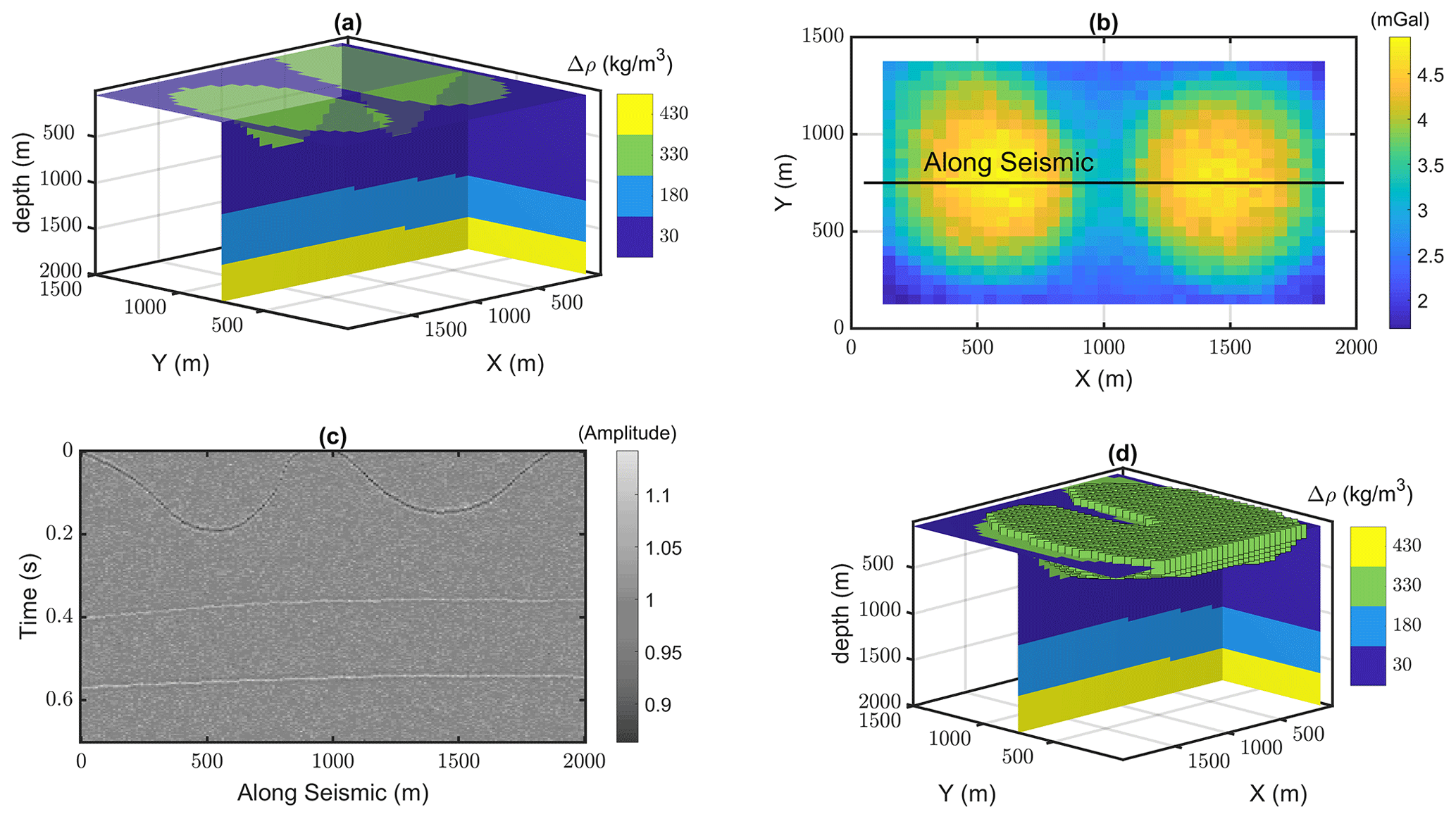
Figure 4 A 3D view of the true model (a) and surface gravity anomaly response (b), a zero-offset synthetic seismic section (c), and a 3D view of the starting model (d).

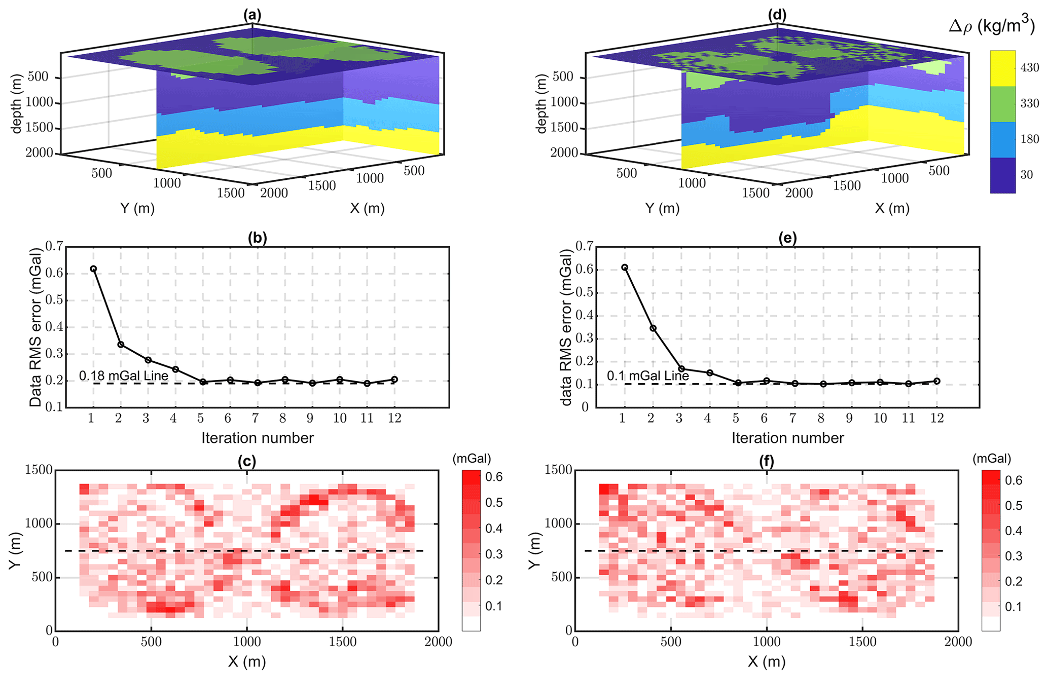
Figure 5 Final inverted models from the seismically constrained (a) and unconstrained inversion (d), evolution of the data RMSE during constrained (b) and unconstrained inversion (e), and the corresponding differences between the calculated data and synthetic observed data, respectively (c, f).

To assess the influence of seismic-derived constraints, we repeat the level set inversion without applying the constraints along the section. The resulting model of 3D gravity inversion without seismic constraints is illustrated in Fig. 5d, with an overall misfit of 0.10 mGal in data root-mean-square error (RMSE) (Fig. 5e).

A comparison of final models from constrained and unconstrained inversion is presented in Fig. 6. The model differences between inverted models and the true model in Fig. 6c and d show more improvement in the constrained case. Model RMSE shows lower values for the constrained inversion (72.5 kg m⁻³). We also compare the results by measuring the structural similarity between the inverted models and the true model. A measurement for structural similarity (SSIM) (Wang et al., 2004) that models the perceived changes in structural information of two different models (A and B) can be used as an indication of changes in the unit boundary locations after level set inversion.

$$\begin{array}{}\text{(7)}& \mathrm{SSIM}\left(\mathrm{A},\mathrm{B}\right)={\displaystyle \frac{\left(\mathrm{2}{\mathit{\mu }}_{\mathrm{A}}{\mathit{\mu }}_{\mathrm{B}}+c_{\mathrm{1}}\right)\left(\mathrm{2}{\mathit{\sigma }}_{\mathrm{AB}}+c_{\mathrm{2}}\right)}{\left({\mathit{\mu }}_{\mathrm{A}}^{\mathrm{2}}+{\mathit{\mu }}_{\mathrm{B}}^{\mathrm{2}}+c_{\mathrm{1}}\right)\left({\mathit{\sigma }}_{\mathrm{A}}^{\mathrm{2}}+{\mathit{\sigma }}_{\mathrm{B}}^{\mathrm{2}}+c_{\mathrm{2}}\right)}}\end{array}$$

$$C_{\mathrm{1}}={\left(K_{\mathrm{1}}L\right)}^{\mathrm{2}},C_{\mathrm{2}}={\left(K_{\mathrm{2}}L\right)}^{\mathrm{2}}$$

Here μ and σ are the mean and variance of two models respectively, σ_AB stands for the covariance of two models, K₁ and K₂ are two small constant values, and L is the dynamic range of the density contrast values. For two identical models, SSIM will become 1. The results indicate that final generated models from seismically constrained gravity inversion have recouped structural features of the true model by up to 65 %. Although the unconstrained inversion leads to a lower data misfit error, the structural similarity between the inverted model and true model is less favorable than in the seismically constrained case (33 %). A higher SSIM for the constrained inversion compared to the unconstrained inversion indicates that applying the seismic constraint has resulted in more structural similarity to the true model. This implies that the method can be applied to real-case scenarios where gravity and seismic datasets with different coverages are available.

Figure 6 (a) Inverted model from the constrained inversion along seismic section. (b) Inverted model from the unconstrained inversion along the same section. (c) Difference between the model in (a) and the true model. (c) Difference between the model in (b) and the true model. Below these figures, the corresponding data and model RMSE and SSIM of two models are compared.

4 Case study: Yamarna Terrane (Yilgarn Craton, Western Australia)

4.1 Geology of the area

The importance of Yilgarn Craton to the economy of Western Australia is evident as it consists of numerous granite–greenstone terranes hosting world-class deposits of gold and nickel (Whitaker, 2004). Several terranes are defined in this craton based on geochronological dating of magmatism and further geochemistry analysis (Cassidy et al., 2006; Pawley et al., 2007). The eastern portion of the Yilgarn Craton is the Eastern Goldfields Superterrane, which is divided into four terranes: Kalgoorlie, Kurnalpi, Burtville, and Yamarna (Pawley et al., 2007). The Yamarna Terrane is located in the northeast (Fig. 7). It is proposed that the Yamarna Terrane evolved separately from the original Burtville Terrane based on the different character of volcano–sedimentary events (Pawley et al., 2012). While there are similarities between the Yamarna Terrane and the sequences around Kalgoorlie (a town host to one of the largest gold deposits in the world), the lack of significant historical mineral discovery is at odds with the apparent prospectivity of the region. Complicated mineral exploration by extensive Phanerozoic cover (Lindsay et al., 2020), significant regolith (Anand and Paine, 2002), and poor outcrop encourage new geophysical investigations in this area to unlock the structure permissive for mineralizing processes (Goleby et al., 2004; Lindsay et al., 2020).

Numerous geophysical datasets including regional gravity data and 2D reflection seismic profiles have been collected in this area. However, few studies integrating these data have been done to estimate the 3D structure of the greenstones. The targeted greenstone belts are proximal to a series of major and minor faults and shear zones, which make it necessary to utilize geophysical integration for regional studies to gain a better understanding of these metal hosts. Gravity datasets, despite providing satisfying lateral resolution, are barely capable of estimating the depth of sub-horizontal interfaces. The 2D seismic sections, on the other hand, contain information about deep structures that need complementary datasets to be laterally extended.

4.2 Geophysical datasets

The region of interest was chosen based on primary interpretation of greenstone locations approximated from the 2D seismic section and surface geological mapping so that it covers an area where two major shear zones (Yamarna and Dorothy Hills) and bounded greenstones cross the long seismic section. This region of interest contains more sparse gravity measurements toward Burtville Terrane to the west and Dorothy Hills shear zone to the east (average 10 km spacing), while denser gravity measurements with 2 km spacing are collected around the Yamarna shear zone (Fig. 8). In this study, we use the interpolated regular grid of gravity anomaly data on the surface (from the Geological Survey of Western Australia) with 400 m spacing (easting: 535 000 to 625 000 m; northing: 6 860 000 to 6 900 000 m) including the spherical cap and terrane corrections in the datasets. The chosen area contains part of the reflection seismic data from common depth point (CDP) number 13 500 (easting: 539 639.00; northing: 6 866 100.00 m) to 18 000 (easting: 622 269.00; northing: 6 891 816.00 m) with an approximate average CDP spacing of 20 m.

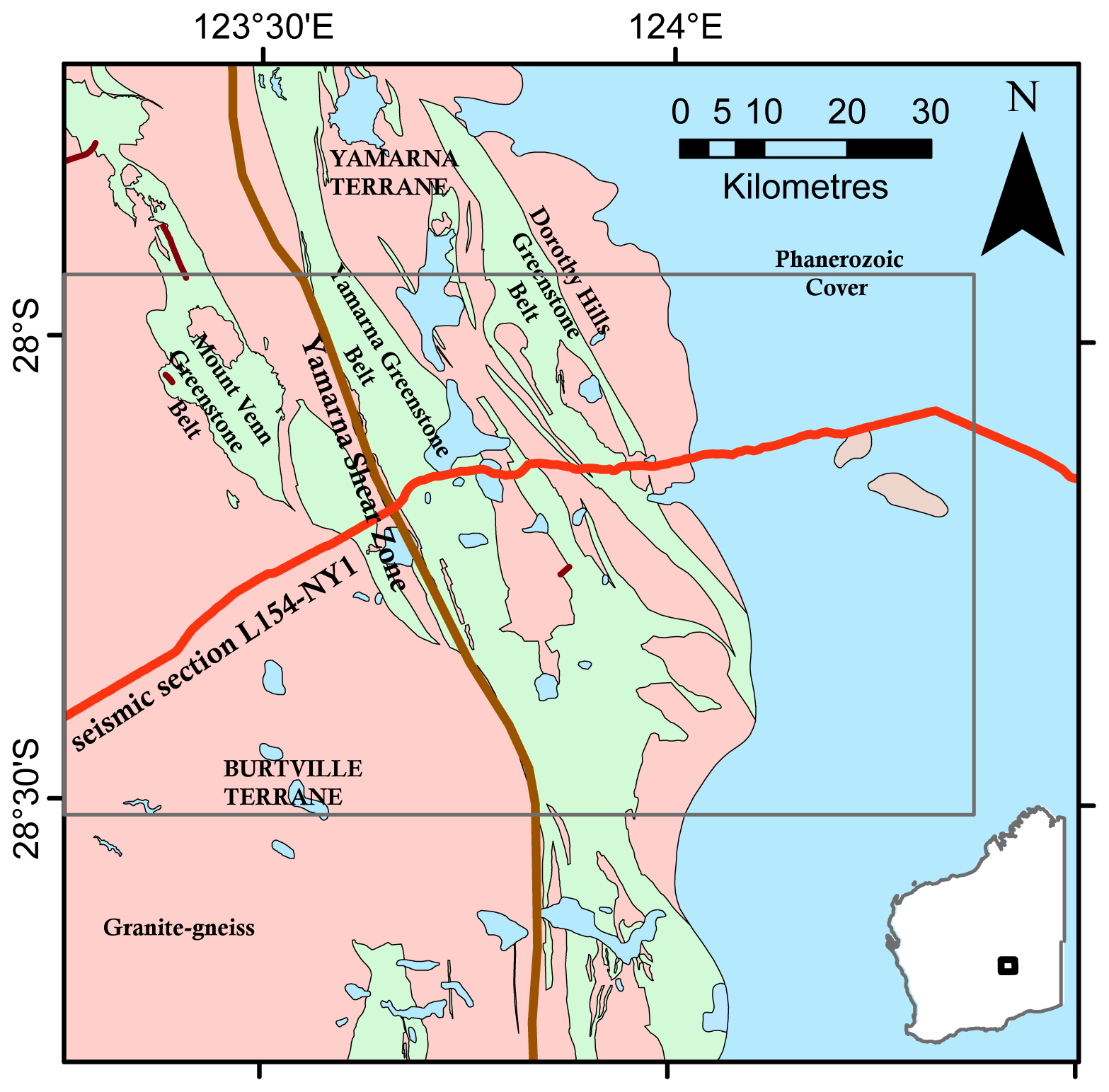
Figure 7 Geographical coordinates and geological units of the region of interest in the Yamarna Terrane, eastern Yilgarn Craton, Albany–Fraser Orogen (modified from Lindsay et al., 2020). The gray rectangle shows the boundary of the region of interest in this study.

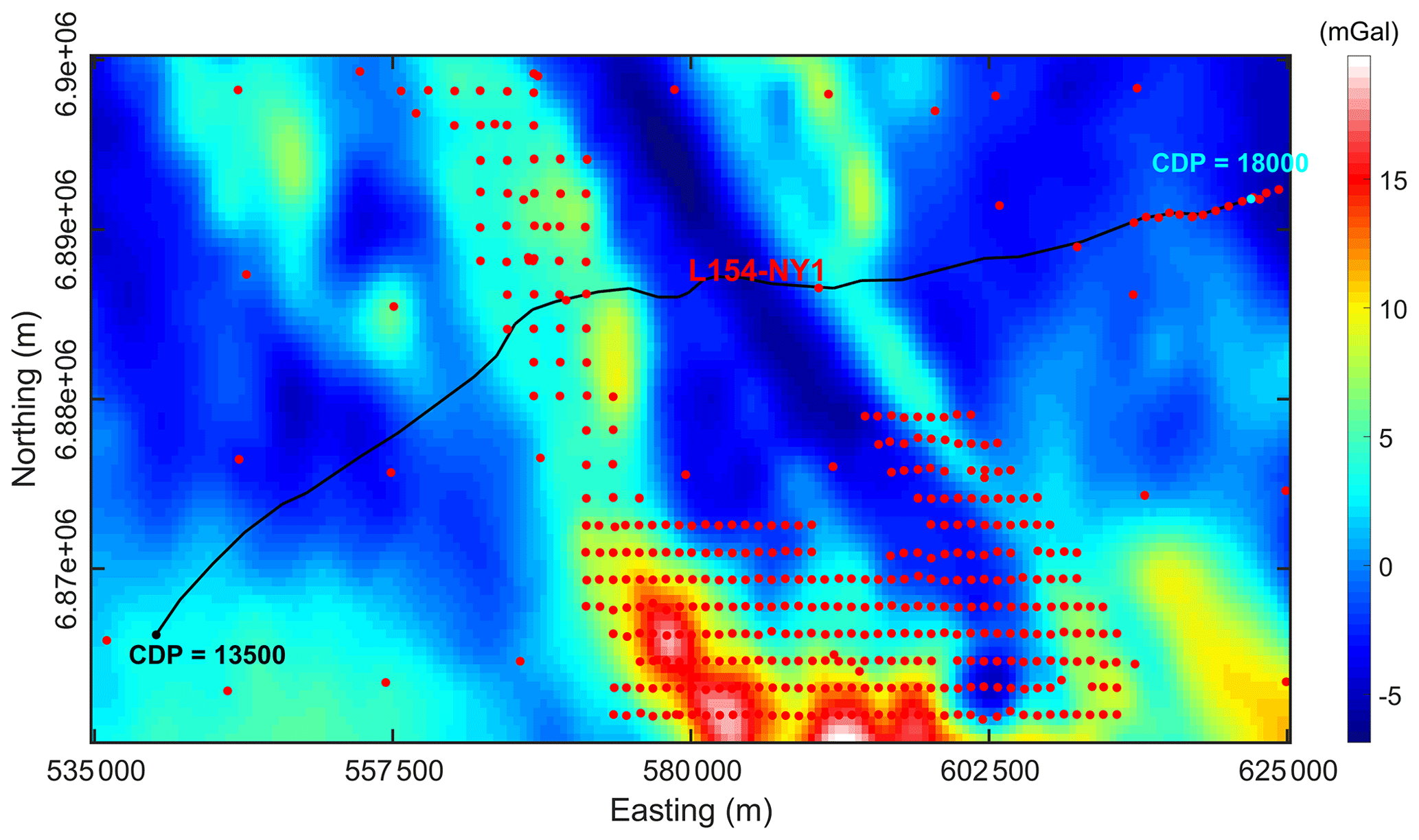
Figure 8 Interpolated gravity anomaly grid of Yamarna Terrane, from Geological Survey of Western Australia. Seismic traverse is shown as a solid black line within the region of interest (from CDP = 13 500 to CDP = 18 000). Red dots indicate the original locations of gravity stations.

4.3 Starting model generation

A general overview of the geological setting of this region based on deep reflection seismic profiling with a focus on Laverton Tectonic Zone modeling is presented in Goleby et al. (2004). Lindsay et al. (2020), on the other hand, put more focus on the integrated multi-scale study of the Yamarna Terrane. Therefore, we use the presented interpretation from Lindsay et al. (2020) for generating a starting model for the inversion.

Referring to primary seismic interpretations from Goleby et al. (2004) and Lindsay et al. (2020), major shear zones hardly extend deeper than 8 km in depth. Focusing on the upper 8 km, we remove the effects of the regional gravitational trend and recalculate the residual Bouguer anomaly (Gallardo and Thebaud, 2012). Therefore, we generate a model grid from the surface down to 10 km depth and discretize to 500 m resolution with cubic cells.

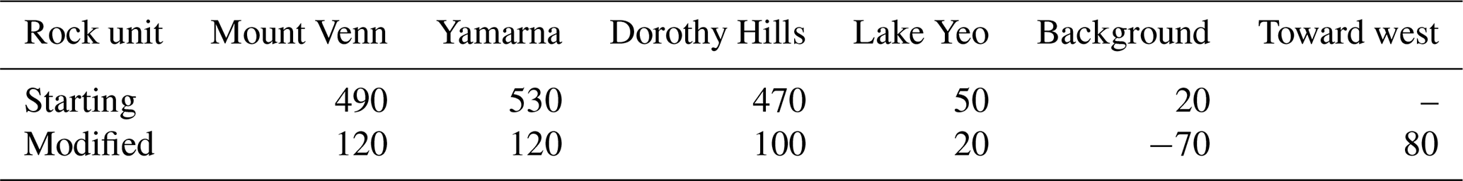
Due to the insufficient number of studies in the region, we mostly rely on the results from a multi-scale study presented in Lindsay et al. (2020) to generate the starting model. In this report, diverse geophysical datasets are utilized to conclude a general integrated interpretation of the region. The presented results from magnetotelluric modeling, reflection seismic reprocessed image and potential field gravity inversion are used for geoscientific investigation. These results from the geophysical modeling are then used to relate petrophysical signatures to geological units using machine learning techniques. We initialize the density contrasts (with the base density of 2670 kg m⁻³) based on a primary gravity anomaly interpretation provided in the report as shown in Fig. 9a. The density contrast values assigned to defined units are inferred from the same report and summarized in Table 1 (first row). For more details about the integrated interpretation of the region, we refer the readers to Lindsay et al. (2020).

Figure 9 (a) Prior model for the gravity property inversion, (b) gravity density contrast inversion result along seismic profile, (c) comparison of the field data and calculated gravity anomaly from the final inverted model, and (d) the overlaid gravity inversion result on seismic profile.

The ultimate aim of this case study is to produce a 3D model from the seismically constrained level set inversion that is consistent with the surface gravity anomaly while including detectable (and thus plausible) structures from the 2D seismic section. To achieve this ambitious aim, we first break down the workflow to 3D property inversion followed by the unconstrained and constrained 3D level set inversions.

4.4 Modifying the starting model

We use the generated knowledge-driven model as the prior model for the density contrast inversion. The Tomofast-x inversion platform (Giraud et al., 2021b, 2020, 2019a; Martin et al., 2020) is used for the property gravity inversion with smallness constraints from the prior model. The inverted density contrast model and the resulting calculated datasets together with the seismic overlaid image are shown in Fig. 9b to d.

Before level set inversion, we modified the starting model based on the property inversion results and utilized the resulting model (Fig. 10) for the 3D level set inversion. The main motivation for modifying the starting model based on the property inversion result is to generate a subsurface model that follows both geophysical datasets and also complements the prior geological knowledge of the region. We tie all this information together and obtain a geologically and geophysically plausible updated model of the area. In this modified model, we assign the same density contrast values to the Mount Venn and Yamarna greenstones and consider them as a single density contrast rock unit as suggested from the property inversion results. In addition, we propose an alternative scenario where we added another density contrast rock unit to the west as derived from the property inversion result. Primary 3D level set inversion of the region of interest using the initially defined starting model strongly suggests the generation of a new rock unit to the west with different dipping from the general east-dipping structure of the area. This appended unit to the west can also be inferred from the seismic image (Fig. 9d), where there are some flat-dipping heterogeneities toward the west edge. We assign a data-driven density contrast heterogeneity to the unit toward the west of the model based on the property inversion results. The ultimate density contrast values used for generating the modified starting model are summarized in Table 1. This modified model is then used as the starting model for the 3D level set inversion of the region, forming five distinct level set functions. The traversed seismic section in the region of interest covers all five defined rock units in the region (Fig. 10b). Furthermore, the modified starting model along this line is utilized for constraining purposes. Out of convenience, we use the section view of the model along the seismic profile for most of the visualization purposes.

Figure 10 Density contrasts of the adjusted starting model and the interpolated gravity grid configuration (a) model cell centers of the extracted 2D model along the seismic profile (b).

The discussion over testing different ranges of density contrast values for different rock units is beyond the scope of this study. However, several sets of density contrasts based on generating a similar range of forward gravity datasets with the field datasets have been tested. In the followings sections, we present the results of one set of the resulting geometries (using the densities in the second row of Table 1) because we note that we recover very similar structures by using different density contrast ranges.

Table 1 Density contrasts assigned to different rock units (units: kg m⁻³).

4.5 Level set inversion in 3D

The aim of this section is to illustrate the application of the gravity level set inversion algorithm to constrain the 3D density model of the area with the seismic section. The starting model for the 3D level set has five distinct units with densities as shown in Fig. 10. The model size for the 3D inversion is $n_x\times n_y\times n_z=\mathrm{180}\times \mathrm{80}\times \mathrm{20}$ = 288 000, and the data size is $N_X\times N_Y=\mathrm{50}\times \mathrm{20}=\mathrm{1000}$. As stated earlier in this section, very little is known about the area, and the generated starting models are highly uncertain. Therefore, the results presented in this section are also undetermined and need to be interpreted with caution. The calculated gravity anomaly responses from the starting model and a comparison with the field datasets are shown in Fig. 11. A very high misfit between the observed and field datasets indicates that existing interpretations are far from reality.

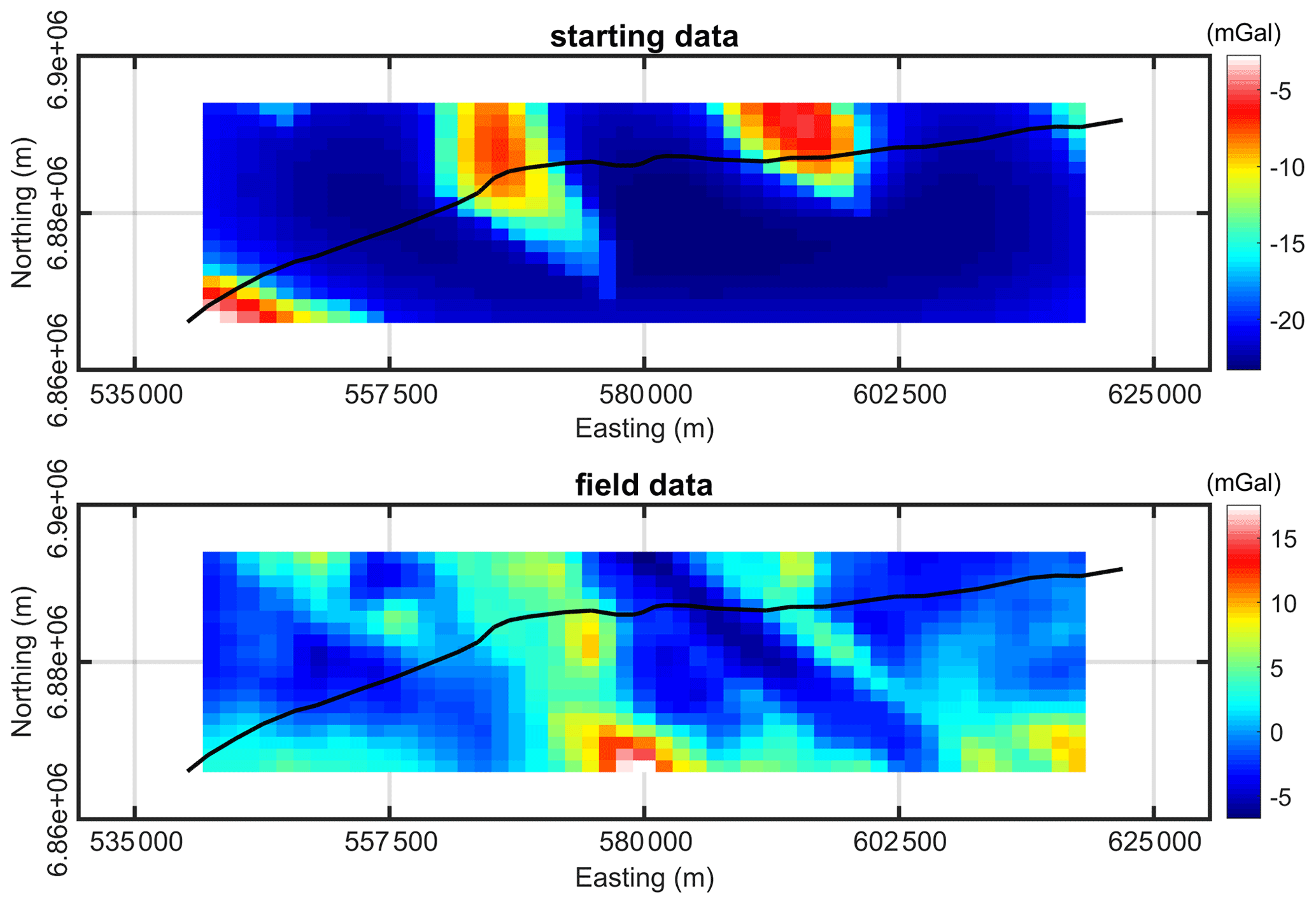
Figure 11 The starting and field gravity datasets of the Yamarna Terrane. Solid black lines represent the seismic traverse.

4.5.1 Unconstrained 3D level set inversion

We first implement the level set inversion without applying constraints along the seismic profile to compare the resulting model from level set inversions with and without seismic information. In this scenario, uniform local and global regularization vectors are appended to the sensitivity matrix without including the weighting from seismic information. We set all regularization parameters to 1 except for the layer at the surface level where we assign a small number (500) to the weighting terms to include information from geological mapping. Morphological closing is also applied as previously introduced using a structuring element of size ($\mathrm{400}\times \mathrm{400}\times \mathrm{400}$ m³). The depth-weighting term for compensating the decay of the gravitational force with depth is also added to the inversion problem as introduced and utilized in Boulanger and Chouteau (2001). The data RMSE of the unconstrained level set inversion decreases smoothly, converging at 1 mGal after 13 iterations (Fig. 13a). The small number of iterations for reaching the optimum value of the data RMSE is due to choosing a relatively broad interface between rock units (τ=2100 m). We previously discussed the importance of this parameter to control the search space of the problem in the theory section. Choosing such a large value for τ allows for rapid convergence given the size of the model.

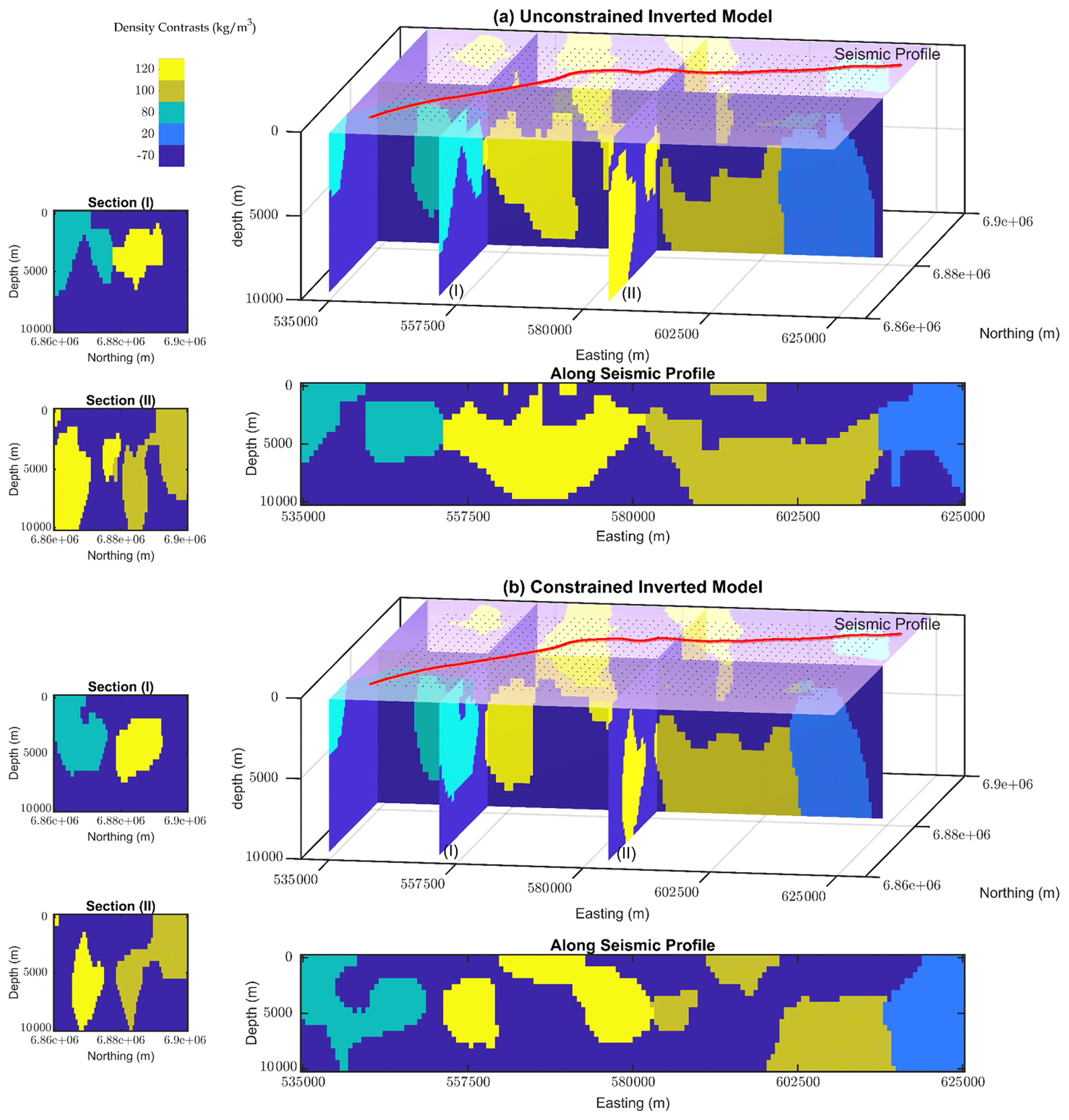
Figure 12 Different views of the final inverted models from the unconstrained and constrained 3D gravity level set inversion of Yamarna Terrane, respectively. Black dots at the surface level represent the interpolated gravity data.

Figure 13 Evolution of data RMSE for the unconstrained (a) and constrained (b) 3D level set inversion of Yamarna Terrane.

The geometry of the density units of the resulting model is, however, not in agreement with the existing geological map and seismic interpretations. The final modeled geometry of the greenstones from the unconstrained inversion is shown in Fig. 12a. These geometries are terminated near the surface and are not extended to depth. This is mainly because we do not apply the constraints at depth. Therefore, the application of the regularizations from the seismic profile to improve the integrity of the units as they evolve laterally (as observed in the interpolated gravity grid) and vertically (as interpreted from the seismic profile) is necessary.

4.5.2 Constrained 3D level set inversion

Next, we apply the spatial constraints along the seismic profile to constrain the gravity inversion with the primary interpretation along seismic section. We aim at reconciling gravity inversion with seismic interpretation. For constraining the inversion along seismic section we rely on interpretations provided in Lindsay et al. (2020) to generate the constraints. We use the same morphological constraints and depth weighting as we set for the unconstrained inversion in order to provide a fair comparison with the unconstrained inversion result. We also use the same value for the τ parameter. The updated regularization terms with weighted constraints from the seismic information along the vertically extended profile are then applied to constrain the inversion. All arrays of the W_s vector are set to 1, except along the seismic section and for the layer at the surface level, which we set as 2000 and 500, respectively, to suppress the changes of the signed-distance function and to constrain the inversion problem with spatially distributed regularizations. The weighting constants are tuned manually during the level set inversion. As a rule of thumb, these constants are chosen to be between 2 and 4 times the cell size. When starting from a significant data root mean square (more than 20 mGal), it repeatedly takes 12 iterations (Fig. 13b) for the data RMSE to reaches the minimum value (1.4 mGal). The final modeled geometry of the greenstones from the constrained inversion is also shown in Fig. 12b.

Comparing the final model from the inversion (Fig. 12b) and the prior model (Fig. 10), we can observe that the geometry of greenstones along the seismic profile is well constrained and the surface features also align with the observed gravity datasets (Fig. 14). Most parts of the inverted model are in line with the existing assumptions in the area and represent an updated geometry for greenstone units adjacent to the shear zones. There are differences between these two models along the seismic section, while the general trend of features away from the seismic profile for both constrained and unconstrained scenarios show very similar patterns. This is an indication of the capability of the approach to apply the constraints along a vertical section and constrain the gravity inversion with sparsely distributed information within the model.

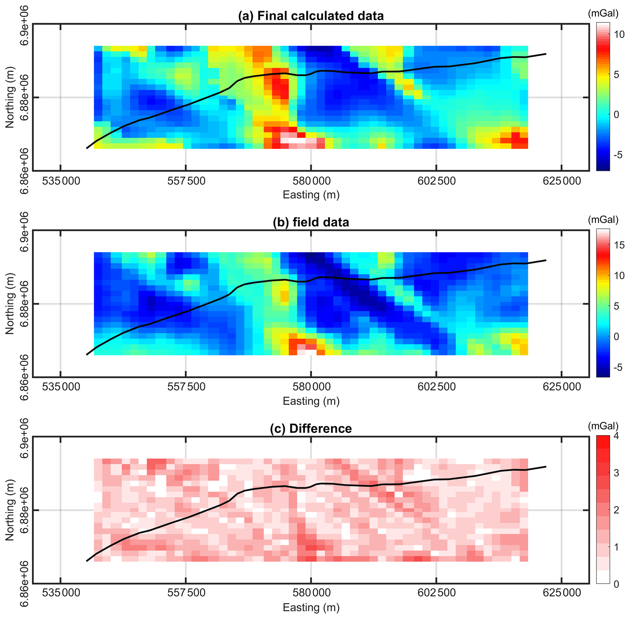
Figure 14 (a) Calculated data from the final constrained inverted model (b) field data and (c) the absolute difference. Solid black lines represent the trace of seismic profile.

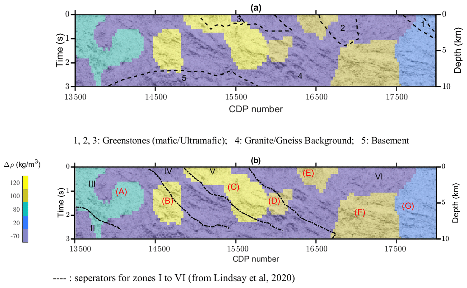
Figure 15 (a) Overlaid final inverted model from the constrained 3D level set inversion with the seismic image and existing primary interpretations in Goleby et al. (2004) (zones 1 to 5). (b) Overlaid model with integrated interpretations based on seismic characters in Lindsay et al. (2020) (zones I to VI). Notation in red (from A to G) indicates distinct units in the resulting model from the constrained inversion.

Figure 15a displays the results of the constrained inversion and recovered geometries along the seismic profile with the interpretation of Goleby et al. (2004) overlain. As demonstrated in Fig. 15, the recovered geometry of the greenstones can be correlated with some detectable features in the seismic image that were not primarily specified. We also provide a comparison of the recovered model with the integrated interpretations provided in Lindsay et al. (2020) in Fig. 15b.

The reason for the difference between these interpretations is mainly that in Goleby et al. (2004) the focus was more on the whole of crust, whereas Lindsay et al. (2020) were looking nearer to the surface and also utilized the reprocessed seismic profile in their study.

5 Discussion

The main focus of this study has been to enable appending spatially distributed constraints in 2D from seismic section to 3D gravity inversion. We have shown this capability across two different synthetic models and a case study to demonstrate different workflows intended for different purposes depending on the available datasets and the area of study.

As detailed in the introduction, seismically constrained gravity inversion has been addressed for a long time. However, constraining gravity inversion quantitatively with sparse seismic information in a cooperative workflow using the level set technique is novel. While we have used information from reflection seismic data as spatially distributed constraints, we see no limitations when using the same approach with other geophysical techniques that provide spatially distributed constraints within the model. For instance, any boundary recognition of rock units from passive seismic, magnetotelluric, or electromagnetic techniques can also be translated to weighted constraints to the level set inversion in the same fashion as we used for reflection seismic data.

The results of the first synthetic study using the salt dome model were presented to demonstrate the application of the approach on a simple model where information from the seismic data is incomplete. The results from the salt dome scenario confirm the applicability of the technique on a simple model where the starting model is far from reality and the constraints are not perfect. The lower body of the salt dome for both the constrained and unconstrained examples is recovered very well after level set inversion, and thus the approach is applicable for imaging subsalt bodies. In addition, the small number of iterations toward convergence using this method is notable compared to other geometrical inversion techniques. This shows that the approach is computationally efficient to be integrated with other approaches (seismic imaging techniques). It can compensate for the poor imaging of salt structures, which has been an issue in the petroleum industry for a long time and is very important in terms of hosting volume accumulation of oil and gas resources. The results of the second and more complex “hard-rock” synthetic model mostly focus on demonstrating the applicability of the technique where more numerous rock units and density contrasts are required. In contrast to the salt dome example, the starting model is closer to the “true” model and allowed closer observation of vertical constraint effects.

The level set method is applied to a part of the eastern Yilgarn Craton, a real-world case study where very little is known about the larger-scale 3D geology of the area. Testing revealed that the constraints generated from the 2D seismic profile and applied to the 3D level set inversion were effective and provided an informative update to the model of the subsurface. The results do not completely disagree with existing crustal interpretations presented in the literature (Goleby et al., 2004; Lindsay et al., 2020). We note that based on our results some new and modified features could be appended to complement existing interpretations. In this area of study, due to the lack of availability of petrophysical datasets, we first implement physical properties inversion followed by the constrained level set inversion. Although simultaneous inversion for density and interfaces would be beneficial in this region, this is not a trivial task and is beyond the scope of this study.

From CDP number 13 500 to 15 000, on the left-hand side of the section shown in Fig. 15, the granite–gneiss outcrop is the main detectable feature on the surface. However, we have assigned a small density contrast value (based on a small gravity anomaly) that also agrees with the moderate east-dipping structures in the seismic image (unit A in Fig. 15b). The main detectable structure from the seismic image is almost compatible with the geometry of the rock units assigned to Yamarna Greenstone Belt (unit C), which in our resulting model is extended by unit D (a unit with the same density contrast as assigned to Dorothy Hills). This almost matches the steep east-dipping structure defined in zone V from Lindsay et al. (2020). Toward the right-hand side of the section shown in Fig. 15, i.e., the Yamarna Greenstone Belt (from CDP 16 700 to 18 000 and from 5 to 10 km), there have been minor interpretations that could explain the flat-lying structures of the seismic image. In the resulting model, these structures are assigned to unit F and unit G, with the same density contrast assigned to Dorothy Hills and Lake Yeo, respectively.

The main detectable feature from the constrained level set inversion as presented in Fig. 12b is the extension of the density contrast that we assign to the Yamarna Greenstone Belt unit that displays a keel-like shape with a dip to the southeast. The western edge of the feature also results in strong reflectors in the seismic image (units C and D in Fig. 15) and has been interpreted to be the Yamarna shear zone (Goleby et al., 2004; Lindsay et al., 2020). Our results indicate that the predicted and modeled Yamarna shear zone aligns with density contrast patterns that follow a anomalously high gravity response laterally away from the seismic survey trace. The results suggest that the greenstone belt extends, along with the shear zone, up to 8 km to the north and south and likely beyond the geographic boundaries of the model.

The other interesting feature from the inverted model that is also in strong agreement with surface geological maps and geophysical information is the depth extension of the Dorothy Hills Greenstone Belt (unit E). Due to the narrow width of this greenstone belt on the surface, the extension of this unit toward deep parts of the model is unlikely. Referring to studies that address greenstone structures in Canada (Thurston, 2015) and Australia (Blewett et al., 2010; Gallardo and Thebaud, 2012), the assumption is that the widths of the greenstone belts are indicative of their depths, which explains the shallow depth of unit E.

A disconnected extension of this unit toward the eastern part of the model, together with the density contrast that we assigned to the Lake Yeo unit, has formed volumes with high-density contrasts (units F and G). This also supports the existing interpretation provided in Lindsay et al. (2020), where they assign a higher-density domain to the eastern side of the Dorothy Hills shear zone.

While our level set inversion results strongly suggest the creation of a density contrast unit with a different dipping structure (unit A) to the west of the model there is a lack of evidence in the literature about the extent of such a density contrast unit. This is mainly because toward the west edge of the model there is a granite–gneiss outcrop and surface geological evidence (Fig. 7, toward Burtville Terrane) fails to confirm the existence of such density contrast in depth. Knowledge about physical properties in a hard-rock environment is not enough to constrain the geological concepts, and the effects of other processes should also be considered (Dentith et al., 2020). This recovered unit is a data-driven unit from observed gravity datasets that lies in an area with a lower density contrast and higher magnetic susceptibility domain based on presented results of gravity and magnetic inversions in Lindsay et al. (2020). These changes in density and magnetic susceptibility might not necessarily support the introduction of a new rock unit and could be an indication of some secondary geological processes (Dentith et al., 2020; Saltus and Blakely, 2011; Whitaker, 2004) that results in local bulk heterogeneities regarding the complex mineral compositions around this region.

Opportunities for improving the presented level set procedure are centered on interpretation and model uncertainty. Firstly, there is considerable uncertainty regarding the appropriate velocity model used during the seismic imaging process utilized within the level set algorithm. Some existing potential field geophysical inversion methods (Giraud et al., 2019a, 2018) use uncertainty as a constraint, and integration with reflection seismic data would help resolve more complicated scenarios involving sparse data, limited petrophysical contrasts, and inadequate model assumptions. In structurally complex areas such as in hard-rock scenarios, there are high uncertainties regarding the local and regional interpretations and the seismic imaging techniques. This indicates the necessity of quantified inclusion of uncertainty regarding the interpretation and imaging process of seismic data when constraining the level set inversion of potential field datasets. It suggests the development of a new technique that enables interactive constraining of the potential field and reflection seismic datasets within a level set algorithm. One advantage of enabling this type of integration in the level set framework is the compatibility of the results with implicit geological modeling. Seismic interpretations and gravity datasets are both very common datasets for generating 3D models of an area, whereas there is no technique that allows for including seismic uncertainty within 3D integrated implicit modeling algorithms.

The presented results of different datasets revealed that constraining level set inversion with sparse constraints from low-uncertainty datasets can effectively improve the (geological) plausibility of the results. Adding constraints to the level set inversion seemed to be effective in all scenarios and is even more obvious with the increasing complexities in the models. Sparse constraints, for which we see no limitations in terms of their source, force the inverted models to retain the available prior knowledge of the area to a high degree. This introduces a resulting model incorporated from several sources of geological and geophysical information and is a step toward automating the process of 3D geo-modeling.

6 Conclusion

We have presented the utilization and extension of a generalized level set approach for seismically constrained gravity inversion across different scenarios. The flexibility of the level set approach we followed allowed us to append 2D constraints from spatially distributed seismic information to 3D level set gravity inversions. We tested the method on two different synthetic models with different scenarios and levels of complexity. The proposed technique was then applied to the geologically complex Yamarna Terrane, and an updated model of the area with supporting discussions was provided. The proposed approach has proven to be reliable to quantitatively include sparse constraints with low uncertainty to the level set inversion. In addition, there is considerable flexibility regarding the constraints, which makes the approach widely applicable for integrating with other geophysical datasets and geological models. The availability of other sources of information in the studied area about the depth of interfaces in the future can also be utilized in this framework for possible modifications of the recovered model. In addition, any improvement in the interpretation of the seismic profile based on future evidence can be directly injected into the inversion to improve the final recovered model.

Appendix A

This appendix presents the definition of some essential elements, with the corresponding equations taken directly from Giraud et al. (2021a) to better understand the material provided in this paper.

The signed-distance function is a signed-distance value (ϕ) that is defined as in Eq. (A1).

$$\begin{array}{}\text{(A1)}& {\mathit{\varphi }}_k\left\{\begin{array}{l}>\mathrm{0}\mathrm{inside}\mathrm{unit}k,\\ =\mathrm{0}\mathrm{at}\mathrm{the}\mathrm{interface},\\ <\mathrm{0}\mathrm{outside}\mathrm{unit}k,\end{array}\right.\end{array}$$

The smeared-out Heaviside function (Osher and Fedkiw, 2003) is a continuous approximation of a Heaviside function as described below:

$$\begin{array}{}\text{(A2)}& H\left({\mathit{\varphi }}_k\right)=\left\{\begin{array}{ll}\mathrm{0}& \mathrm{if}{\mathit{\varphi }}_k<-\mathit{\tau },\\ \frac{\mathrm{1}}{\mathrm{2}}+\frac{{\mathit{\varphi }}_k}{\mathrm{2}\mathit{\tau }}+\frac{\mathrm{1}}{\mathrm{2}\mathit{\pi }}\sin \left(\frac{\mathit{\pi }{\mathit{\varphi }}_k}{\mathit{\tau }}\right)& \mathrm{if}\mathrm{0}\le \left|{\mathit{\varphi }}_k\right|\le \mathit{\tau },\\ \mathrm{1}& \mathrm{if}{\mathit{\varphi }}_k>\mathit{\tau },\end{array}\right.\end{array}$$

where τ defines the maximum distance from the interface between rock units.

The model in this approach is defined such that rock units are defined everywhere in the model by a given ϕ>0:

$$\begin{array}{}\text{(A3)}& \mathit{m}\left({\mathit{\varphi }}_{\mathrm{1}},\mathrm{\dots },{\mathit{\varphi }}_N\right)=\sum _{k=\mathrm{1}}^N\left[V_{k}H\left({\mathit{\varphi }}_k\right)\prod _{\left\{\begin{array}{l}j=\mathrm{1}\\ j\ne k\end{array}\right.}^N\left(\mathrm{1}-H\left({\mathit{\varphi }}_j\right)\right)\right],\end{array}$$

where V_k is the physical property value of the kth rock unit such that $\mathit{V}=\left[V_{\mathrm{1}},\mathrm{\dots },V_N\right]$ contains all possible values a given model cell can take; H is the Heaviside function.

The sensitivity of the geophysical datasets to the interface location is calculated as in Eq. (A4):

$$\begin{array}{}\text{(A4)}& {\mathbf{J}}_{ij}^{{\mathit{\varphi }}_k}={\mathbf{J}}_{ij}^m{\displaystyle \frac{\partial m_j}{\partial {\left({\mathit{\varphi }}_k\right)}_j}},\end{array}$$

where ${\mathbf{J}}_{ij}^m$ is the sensitivity of the ith measurement to the variation of m in the jth model cell, and ${\mathbf{J}}_{ij}^{{\mathit{\varphi }}_k}$ is the sensitivity of the ith measurement to the variation in the signed-distance ϕ_k in the jth model cell.

Figure A1 Illustration of the signed-distance function for density contrast of a single rock unit. Modified from https://en.wikipedia.org/wiki/Signed_distance_function (last access: 16 October 2021).

Appendix B

This appendix presents the effect of applying topological rules as morphological closing in the level set problem. We have used the top view of the second synthetic example within this paper to illustrate this effect.

Figure B1 Top view of the hard-rock synthetic example at the depth of 150 m. Panels (a) and (b) show the results of the unconstrained inversion without applying the morphological closing to the model and after applying the morphological closing constraint, respectively.