the Creative Commons Attribution 4.0 License.
the Creative Commons Attribution 4.0 License.
 | 09 Nov 2021
Very early identification of a bimodal frictional behavior during the post-seismic phase of the 2015 Mw 8.3 Illapel, Chile, earthquake
Cedric Twardzik
Mathilde Vergnolle
Anthony Sladen
Louisa L. H. Tsang
It is well-established that the post-seismic slip results from the combined contribution of seismic and aseismic processes. However, the partitioning between these two modes of deformation remains unclear due to the difficulty of inferring detailed and robust descriptions of how both evolve in space and time. This is particularly true just after a mainshock when both processes are expected to be the strongest. Using state-of-the-art sub-daily processing of GNSS data, along with dense catalogs of aftershocks obtained from template-matching techniques, we unravel the spatiotemporal evolution of post-seismic slip and aftershocks over the first 12 h following the 2015 Mw 8.3 Illapel, Chile, earthquake. We show that the very early post-seismic activity occurs over two regions with distinct behaviors. To the north, post-seismic slip appears to be purely aseismic and precedes the occurrence of late aftershocks. To the south, aftershocks are the primary cause of the post-seismic slip. We suggest that this difference in behavior could be inferred only a few hours after the mainshock. We finish by showing that this information can potentially be obtained very rapidly after a large earthquake, which could prove to be useful in forecasting the long-term spatial pattern of aftershocks.
- Article
(4566 KB) - Full-text XML
-
Supplement
(27310 KB) - BibTeX
- EndNote


One of the most perceptible expressions of the post-seismic activity following a large earthquake is the occurrence of aftershocks. To the first order, their temporal behavior is well-described by the Omori–Utsu law (Omori, 1894; Utsu et al., 1995), which states that the frequency of aftershocks decays as a power law with time after the mainshock. Although widely accepted, its physical origin is still debated. For instance, Miller (2020) proposes that the decay rate of aftershock sequences reflect the ability of the medium to heal co-seismic and post-seismic perturbations, influencing the circulation of fluids and consequently the temporal evolution of aftershocks. The geometrical complexity of the fault zones has also been proposed to explain the emergence of the Omori–Utsu law for aftershock sequences (Ozawa and Ando, 2021). On the other hand, it has also been argued that power laws might not be suited to explain the temporal evolution of aftershocks with, for instance, Mignan (2015) suggesting that stretched exponential functions fit the observations better.
As for the spatial distribution of aftershocks, we know since the mid-1950s that it is somehow linked to the rupture area of the mainshock (Utsu and Seki, 1954). A first-order spatial forecast can be made by stating that fewer aftershocks will occur in areas of large co-seismic slip (e.g., Das and Henry, 2003; Wetzler et al., 2018). But the most common approach is to forecast the spatial extent of aftershocks based on the regions that experience positive Coulomb stress changes from the mainshock (e.g., Das and Scholz, 1981; Kirb et al., 2002). In particular, this can explain the observed spatial decay of aftershocks (e.g., van der Elst and Shaw, 2015). However, it has also been shown to fail for a certain number of cases (see Mallman and Zoback, 2007). Therefore, other routes have been explored such as using different stress metrics (e.g., the invariants of the stress tensor or the maximum shear – Meade et al., 2017) or analyzing the influence of other attributes of the mainshock as proxy for aftershock productivity (e.g., radiated seismic energy, stress drop, slip heterogeneity – Dasher-Cousineau et al., 2020).
Another potential mechanism that could explain both the spatial and temporal evolution of aftershocks might lie within the post-seismic phase. Thanks to geodetic measurements, we know that the post-seismic deformation does not only express itself in the form of aftershocks, but also with aseismic slip on the fault, hereafter called afterslip (e.g., Heki and Tamura, 1997). Some studies even suggest that it is the main driving mechanism of aftershocks (e.g., Perfettini and Avouac, 2007; Peng and Zhao, 2009; Ross et al., 2017; Perfettini et al., 2018b, 2019). Based on that hypothesis, afterslip could be used to forecast the location and timing of aftershocks. The fact that only the modeling of afterslip would be necessary could help limit the sources of errors when compared to stress-based approaches which require two steps (and hence potentially two sources of error): the modeling of the slip distribution of the mainshock and that of the Coulomb stress changes. In addition, an approach based on afterslip offers the possibility to monitor temporal changes.
One issue with the latter approach is that the geodetic surface observations record the combined contribution of seismic and aseismic slip on the fault. Therefore, it is crucial above all to understand how these two regimes are partitioned during the post-seismic phase. Most of the previous studies that have investigated such issues have used daily GNSS (Global Navigation Satellite System) position time series, thus focusing on a time period starting at least from ∼ 12 to 24 h after the mainshock (e.g., Lange et al., 2014). Because of this, very little is known in the time window starting from the first minutes and up to the first few hours after the mainshock. For instance, is afterslip the driving mechanism of aftershocks even during the very early stage of the post-seismic phase? Or, is the ratio between seismic and aseismic slip at this very early stage of the same order as what is observed at longer times?
Over the last few years, precise geodetic observations of the very early post-seismic phase with high temporal resolution have emerged (Langbein et al., 2006; Miyazaki and Larson, 2008; Munekane, 2012; Malservisi et al., 2015; Twardzik et al., 2019; Milliner et al., 2020; Jiang et al., 2021), allowing us to investigate specifically these first 12 h. At the same time, the development of advanced detection techniques using seismological data has led to the construction of more complete aftershock catalogs (e.g., Wang et al., 2017; Shelly, 2020). These methods are particularly effective in detecting earthquakes very early after a mainshock, a somewhat challenging task because numerous aftershocks occur very close in time at this stage, and the signal can be contaminated by surface waves or the coda of the mainshock or previous large events. This is a critical step since the use of incomplete catalogs can lead to distorted results (Hainzl, 2016). By combining these more complete catalogs with geodetic observations of high temporal resolution, we can now study in detail the relationship between aftershocks and afterslip at the very early stage of the post-seismic phase.
To this end, we investigate the first 12 h following the 16 September 2015, Mw 8.3, Illapel, Chile earthquake, for which GNSS position time series with high temporal resolution are available (Twardzik et al., 2019) as well as dense catalogs of aftershocks obtained from template-matching techniques (Frank et al., 2017; Huang et al., 2017). First, we analyze the geodetic surface observations to obtain hourly images of the afterslip distribution over these first 12 h, and we compare that with the spatiotemporal evolution of aftershocks. Then, we estimate the seismic–aseismic slip partitioning over this time period to better understand the mechanical behavior of the subduction interface just after the mainshock. Finally, we discuss the potential of using very early afterslip observations for the forecast of the spatial patterns of aftershocks.
2.1 Geodetic data
On 16 September 2015, a Mw 8.3 earthquake occurred near the city of Illapel in central Chile. It ruptured part of a locked segment of the south American subduction zone that is surrounded by two areas of relatively low coupling (Ruiz et al., 2016). Thanks to the Centro Sismológico Nacional (CSN) of the University of Chile, this region was heavily instrumented with GNSS stations at the time of the earthquake (Baez et al., 2018). Thus, we have access to 15 high-rate GNSS stations that are located < 350 km from the earthquake epicenter (Fig. 1). To investigate the first 12 h following the mainshock, we first need to obtain sub-daily position time series. For that, we used the 30 s 3-component kinematic position time series starting just 5 min after the origin time of the mainshock from Twardzik et al. (2019). To reduce the high-frequency noise, a Kalman filter, which was tuned to be suitable for detecting slow processes over timescales of hours to days (Choi, 2007), was used during the processing of the GNSS data. Then, these time series were post-processed by applying a sidereal filter constructed in such a way that it can remove periodic noise without removing the post-seismic signal (Twardzik et al., 2019). Finally, we disregarded the vertical component because its noise level is too large (∼ 2 times that of the horizontal components). An example illustrating the post-processing can be found in Fig. 2.
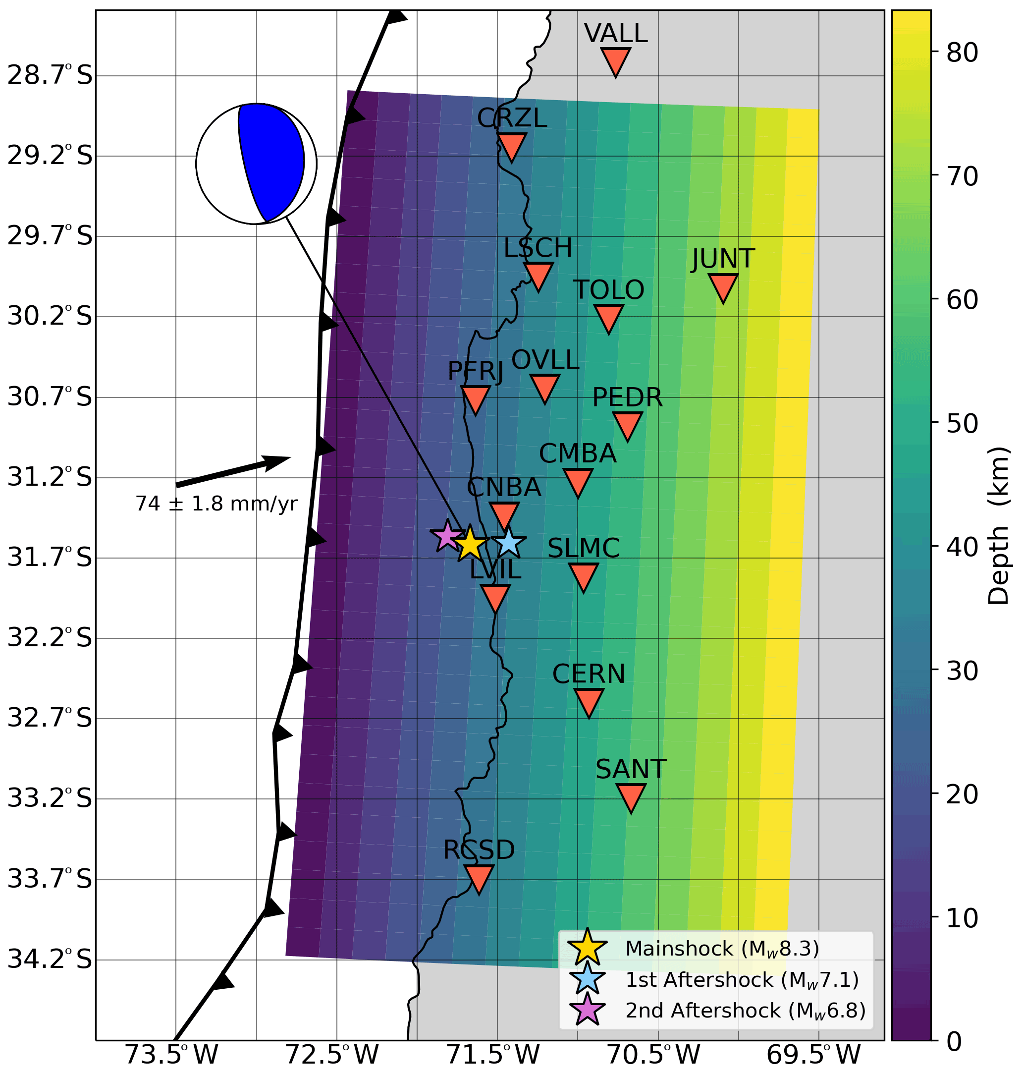
Figure 1Setup used for the post-seismic slip inversions presented in this study. The fault plane (3∘ N of strike and 17∘ dipping angle) is color-coded according to depth. The red triangles are the GNSS stations. The yellow star shows the epicenter of the 2015, Mw 8.3, Illapel, Chile earthquake and it is connected to its focal mechanism retrieved from the United States Geological Survey. The light blue and purple stars show the largest aftershocks reported by the Global Centroid Moment Tensor (GCMT) catalog (Mw 7.1 and 6.8, respectively). The chevron line shows the location of the plate boundary from Bird (2003). Finally, the black arrow shows the plate motion of the Nazca plate with respect to a fixed South America plate (DeMets et al., 2012).
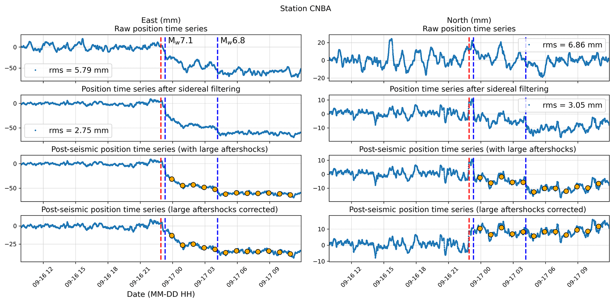
Figure 2Processing steps performed to get the time series used in this study. The first row shows the raw position time series. The mean and a linear trend are calculated using the 6 d prior to the mainshock origin time (red dashed line) and are removed from the time series. We also calculated the root mean square (rms) over that same time period to illustrate the noise level. Note that the static offset of the mainshock is removed. The second row shows the position time series after applying a sidereal filter which is constructed as proposed by Twardzik et al. (2019). This allows the noise level to be reduced by ∼ 35 % across all stations. The third row shows the position time series that we use to obtain the spatiotemporal evolution of the post-seismic slip over the first 12 h (orange dots). Each dot is the average position using a 1 h time window centered on the time of interest and spanning 30 min on either side. The fourth row shows the position time series with the estimated static offsets of the two largest aftershocks removed. In all figures, the blue dashed lines show the two largest aftershocks in the GCMT catalog. Supplement S2 shows a similar figure for all the stations.
Over the first 12 h that followed the Illapel earthquake, two large aftershocks were reported in the Global Centroid Moment Tensor (GCMT) catalog. The first one (Mw 7.1) occurred ∼ 23 min after the mainshock, while the second one (Mw 6.8) occurred ∼ 5.25 h after it. To quantify later in the discussion the impact of these large aftershocks on the post-seismic slip, we calculate their static offsets from the position time series. Because of the Kalman filter, these offsets are smoothed over time and thus are not accommodated instantaneously but instead over a certain duration (Tkalman). That duration can be estimated by the following formula: , where A is the expected amplitude of the static offset at the stations, Δt is the sampling interval of the time series, and k is the parameter of the Kalman filter ( km s−2). We estimate A by computing the expected offsets using Okada's formulas (Okada, 1985) inside an homogeneous half-space (μ=39 GPa for the rigidity and ν=0.25 for the Poisson's ratio) and using the nodal plane with the shallower dipping angle as well as the hypocenter location reported by the GCMT catalog. The expected width and length of the fault plane is determined using the empirical relationship for subduction-interface events obtained by Thingbaijam et al. (2017). From the estimated Tkalman, we extract the static offsets of these two aftershocks from the position time series by choosing a pre-earthquake position at and a post-earthquake position at . We center the offset on the origin time of each earthquake to account for the fact that the Kalman filter is applied both forward and backward. We show in Supplement S1 two tables that summarize the computed offsets at each station for both aftershocks. An example of a corrected time series is presented in Fig. 2.
The kinematic position time series, even after applying a sidereal filter, remain relatively noisy. The standard deviation calculated over the 6 d of data prior to the mainshock ranges from 2.45 to 3.98 mm. Thus, we choose to favor noise reduction over the rate of positioning. Every hour, from the 1st to the 12th hour after the mainshock, we calculate the average position using a 1 h window centered on the time of interest. Thus, we obtain hourly position time series that show the cumulative surface displacement since the mainshock. The errors associated with these new observations are set to the standard deviation of the time series measured prior to the mainshock. Figure 2 illustrates for one station the different steps that we perform to obtain the hourly position time series (see Supplement S2 for similar figures for all the stations). The orange dots in Fig. 2 represent the hourly positions that we use to obtain the spatiotemporal evolution of very early afterslip. Because of strong spurious signals that are not of tectonic origin, we disregard the first two hours for station LVIL and hours 2 and 3 for station OVLL.
2.2 Inversion of the very early afterslip
Using the observations described above, we attempt to obtain the hourly spatial distribution of afterslip on a planar fault that is 600 km long along the strike and 300 km long along the dip (Fig. 1). Our assumed fault geometry has a strike of 3∘ N and is adjusted such that its upper edge coincides with the trench. The fault dip is chosen to be 17∘, which corresponds to the average dip of the slab at this location calculated from the Slab1.0 model from Hayes et al. (2012). Then, the fault is divided into 450 sub-faults, 30 along the strike and 15 along the dip, with the slip amplitude and rake angle evaluated at their centers. We use the approach by Zhu and Rivera (2002) to compute the static response of each sub-fault in a tabular medium obtained from the CRUST1.0 database (Laske et al., 2013). For a given source model, the surface displacements at each receiver are computed by summing the contribution of each sub-fault.
We search for the spatial distribution of slip amplitude and rake angle independently for each time step. For the slip amplitude, we limit the search to values between 0 and 1 m, thus ensuring the positivity of slip. For the rake angle, we only explore values that are plus or minus 15∘ from the rake angle of the mainshock given by the GCMT catalog (i.e., 109∘). Both parameters are drawn from a uniform prior. The spatial distribution of the source parameters is obtained using an optimization procedure similar to that of Pianatesi et al. (2007). We use a heat-bath simulated annealing algorithm, an evolution of the Metropolis–Hastings that lowers the rejection rate by computing the relative probabilities from a set of trial models before a random move is made (Sen and Stoffa, 2013). To measure the difference between the observed (o) and calculated (c) surface displacements, we use the cost function of Pianatesi et al. (2007) to which we add a smoothing constraint:
where N is the number of observations (2 horizontal components × number of receivers), e is the error associated with the observation, Λ is the Laplacian of the slip distribution and ω is the weight given to the Laplacian (0.1 in this study – see Supplement S3 for a discussion on how the value is chosen).
Similarly to Pianatesi et al. (2007), we keep track of the model after each iteration. For each time step, we run the algorithm 100 times, each time with a different random seed, which leads to a slightly different outcome after each run. Thus, we end up for each time step with an ensemble of 40 000 models along with their misfit values. We use this ensemble of models to build an average one along with its standard deviation. Both are computed by weighting the models by the inverse of their misfit, thus giving more weight to best fitting models. Hereafter, we set to zero the sub-faults that have a mean slip amplitude that is smaller than its standard deviation.
Following the procedure described above, and using the time series recording both seismic and aseismic deformation, we obtain hourly post-seismic slip distribution models. This allows us to investigate its spatiotemporal evolution over the first 12 h (Fig. 3). The fit to the observations is shown in Supplement S4, and a sensitivity analysis is done in Supplement S5 to assess the reliability of the post-seismic slip models.
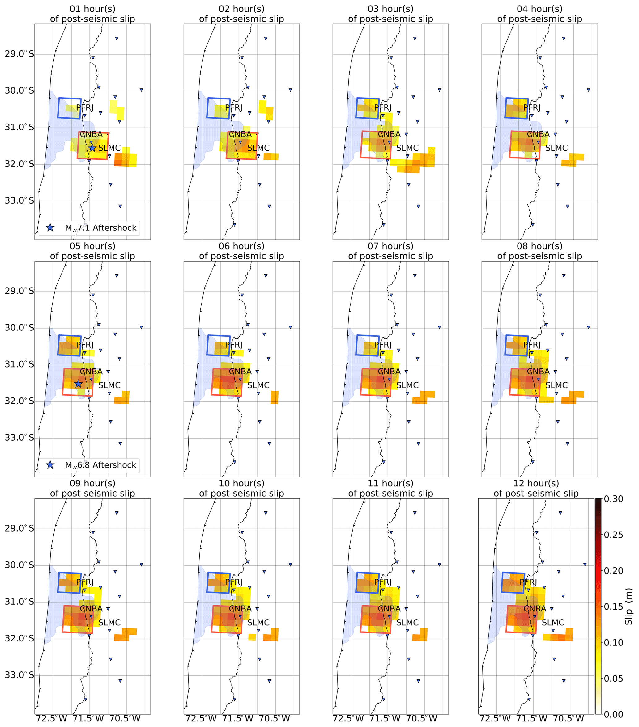
Figure 3Hourly map of the post-seismic slip distribution over the first 12 h after the mainshock. Each model is obtained after averaging 40 000 models, each weighted by the inverse of its misfit value. Sub-faults with slip amplitude lower than the standard deviation are set to 0. The light blue area shows the co-seismic slip region obtained by Melgar et al. (2016). The blue stars show the two largest aftershocks in the GCMT catalog at their time of occurrence. The blue square outlines what we refer to as the northern patch in the text while the red square outlines what we refer to as the southern patch.
Our results show distinct patches that are not moving in space but grow in amplitude over time and can be identified 1 to 3 h after the mainshock. The first one to develop is located near the epicenter of the mainshock (red square in Fig. 3), offshore of Canela Baja (station CNBA). This is also where the two largest aftershocks are located (blue stars in Fig. 3). This patch seems to nucleate at the southern edge of the co-seismic rupture area inferred by Melgar et al. (2016), which is shown as the blue shaded region in Fig. 3. That co-seismic model is chosen because it is mostly based on data recording the co-seismic phase only (i.e., seismological data, high-rate GNSS data, tsunami data), limiting the contamination from very early afterslip by the InSAR data. After 12 h, we find that the geodetic moment of this patch is 3.7 × 10¹⁹ Nm (Mw eq. 7.0). The second patch to develop is located to the north of the co-seismic rupture area (blue square in Fig. 3), offshore of Fray Jorge Park (station PFRJ). Although some slip is seen in this area during the first 2 h (< 0.1 m), this patch starts to grow noticeably in amplitude after 3 h and ends up with a geodetic moment of 1.5 × 10¹⁹ Nm after 12 h (Mw eq. 6.7). In between these two patches, and down-dip of the co-seismic rupture area, a connection starts to robustly build up ∼ 7 h after the mainshock. After 12 h, we find that the entire afterslip model has a geodetic moment of 1.0 × 10²⁰ Nm (Mw eq. 7.3), and it shows a rather continuous region of slip that surrounds the area of co-seismic rupture.
When compared with models of post-seismic slip over longer timescales (from 1 d up to 2 months after the mainshock; see Fig. 4), we find that the bimodal slip distribution persists over time. Thus, it appears that following the Illapel earthquake, the post-seismic slip patches remain at a steady location throughout the first 2 months. Although some studies show hints of afterslip migration (e.g., Jiang et al., 2021), it is more common to find that afterslip remains at a steady location over time as pointed out by Bedford et al. (2013) who reviewed several studies analyzing the spatiotemporal evolution of afterslip. Therefore, as illustrated by our study, information about the very early afterslip could be useful to infer the long-term properties of the afterslip pattern rapidly after the mainshock.
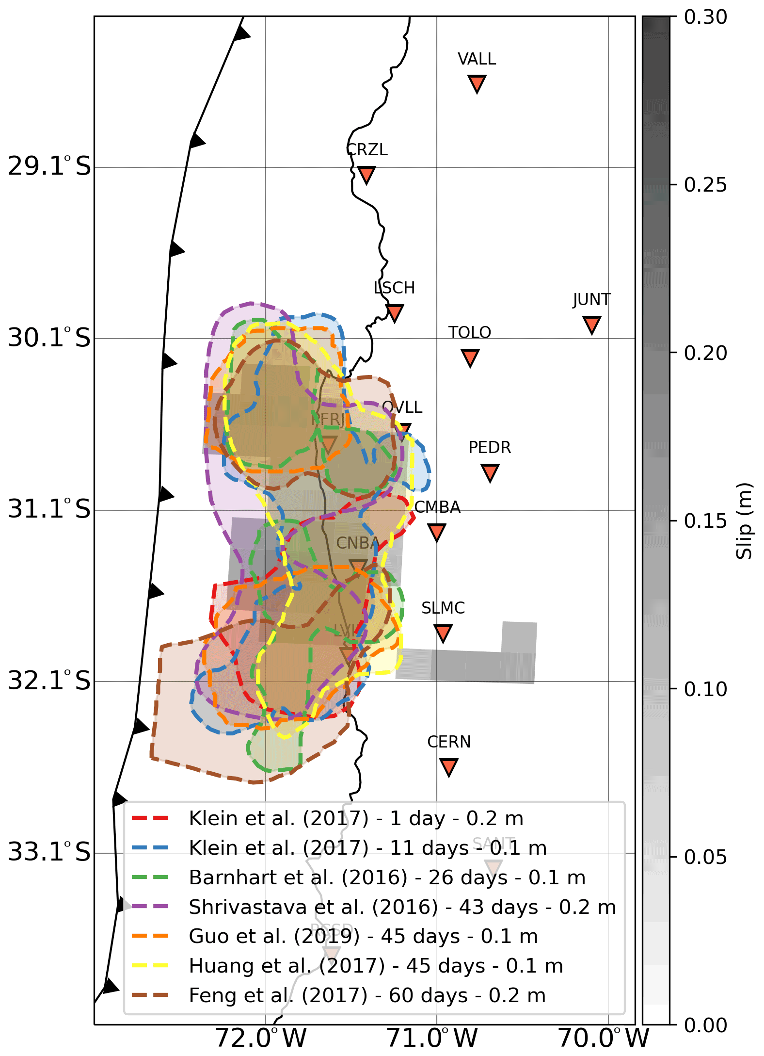
Figure 4Comparison between post-seismic slip 12 h after the mainshock (slip from our study in grayscale) and post-seismic slip from 1 d and up to several weeks after the mainshock (dashed lines). Klein et al. (2017) use GNSS data and look at the shorter time period (1 and 11 d). Barnhart et al. (2016) use both GNSS and InSAR data to model post-seismic slip after 26 d. Shrivastava et al. (2016) use GNSS data to investigate post-seismic slip after 43 d. Guo et al. (2019) also use GNSS data to image post-seismic slip after 1.5 months. The post-seismic slip distribution taken from Huang et al. (2017), using GNSS and InSAR data, is also after 1.5 months. Finally, the model obtained by Feng et al. (2017) uses geodetic data to look at post-seismic slip after 2 months. Numbers beside the references show the slip isoline amount. Symbols are the same as for Fig. 1.
When we look more closely, we see that some of the post-seismic slip might have penetrated inside the co-seismic rupture area (Fig. 3). There have been such observations at the very early stage of the post-seismic phase in particular following the 2008 Tokachi-Oki, Japan, earthquake (Miyazaki and Larson, 2008) and the 2016 Pedernales, Ecuador, earthquake (Tsang et al., 2019). Under the standard rate-and-state friction law framework usually used to explain post-seismic slip, this should be precluded because co-seismic slip is associated with slip-weakening frictional conditions while post-seismic slip is rather associated with slip-strengthening frictional conditions (e.g., Marone et al., 1991). However, this might become possible under certain circumstances. For instance, the frictional properties could be modified because of the redistribution of stresses in the medium after a large earthquake (Helmstetter and Shaw, 2009). This can also occur because of heterogeneities in the mineral composition of fault gouges (Colletini et al., 2011) or complexities in the fault geometry (Romanet et al., 2018). It is also possible that co-seismic slip penetrates significantly into regions exhibiting a slip-strengthening behavior (Salman et al., 2017). When we compare our post-seismic slip model with other co-seismic slip models, as well as with our own co-seismic model, we see that our afterslip model lies at the edges of most of the co-seismic slip models (see Supplement S6). However, depending on which model we choose, the amount of overlap varies significantly. Given the variability of the co-seismic rupture area and the level of uncertainty in our own post-seismic slip models, we find it difficult to reach a definitive conclusion on the matter. This is in line with Barnhart et al. (2016) who discuss this question by looking at 26 d after the mainshock and using a similar dataset to ours (i.e., 9 of the 15 GNSS stations plus InSAR data). They find some overlap between co-seismic and post-seismic slip but also conclude that this result is not robust enough to be interpreted.
Finally, we also identify in our models a region where significant slip occurs that is located southeast of Salamanca (station SMLC). This region is further away from the co-seismic rupture area and is disconnected from the main regions of post-seismic slip. After some tests (see Supplement S5), we conclude that this patch is an unreliable feature and is therefore disregarded in the discussion section. When this region is not taken into account, the final geodetic moment decreases to 8.3 × 10¹⁹ Nm (Mw eq. 7.2).
4.1 Relationship between very early aftershocks and very early post-seismic slip
One of the first points we aim to assess is the relationship in space and time between aftershocks and post-seismic slip right after the mainshock, here during the first 12 h. For that, we compare the spatiotemporal evolution of slip and aftershocks using the catalog compiled by Huang et al. (2017) (see Fig. 5). Although it is possible that some of these aftershocks are not on the subduction interface, based on the focal mechanisms obtained by Carrasco et al. (2019) we can make assumptions at least for regions where we observe afterslip. We find that afterslip and aftershocks show large similarities. Over the first 2 h, most of the seismic activity occurs south of the rupture area, just as does the post-seismic slip. To the north, very little activity is seen during these first 2 h but it then progressively intensifies just like the post-seismic slip. After the first 12 h of the post-seismic phase, we see a pattern where post-seismic slip and aftershocks strongly overlap, both surrounding the co-seismic rupture area. The same observation can be made when we use the independently obtained aftershock catalog by Frank et al. (2017) (see Supplement S7).

Figure 5Hourly map of the post-seismic slip distribution over the first 12 h after the mainshock along with the cumulative aftershocks from the catalog compiled by Huang et al. (2017) and shown with black dots. Detailed caption can be found in Fig. 3.
The strong similarity between these two spatiotemporal evolutions could be due to the fact that the cumulative contribution of aftershocks is not removed from the position time series, thus contributing to the estimated fault slip. For instance, this is what has been proposed to explain the pre-seismic slip pattern prior to the 2014 Iquique, Chile, earthquake (Schurr et al., 2014). This naturally leads to the question of the partitioning between seismic and aseismic slip during the very early post-seismic phase. To investigate this question, we compare the geodetic moment from the post-seismic slip models with the seismic moment released by aftershocks. To estimate the latter, we use the GCMT catalog for the two largest earthquakes and the catalog from the Centro Sismológica Nacional (CSN) of the University of Chile for the smaller earthquakes, restricting to those with available moment magnitude estimates. Thus, over the whole fault plane considered in this study, there are 38 aftershocks with magnitudes ranging from 4.5 and up to 7.1. That leads to a seismic moment released by the aftershocks of 9.5 × 10¹⁹ Nm. This estimate is slightly larger than the geodetic moment of afterslip (8.3 × 10¹⁹ Nm), which we will discuss next. But the fact that the seismic moment released by aftershocks is rather close to the geodetic moment of afterslip would suggest that the post-seismic slip that we have obtained can be imputed to seismic slip rather than aseismic slip. However, we find that there is a very large spatial discrepancy : ∼ 95 % of the seismic moment released by the aftershocks is done in the southern patch, ∼ 0.1 % in the northern patch and ∼ 4.9 % elsewhere on the fault plane.
To investigate that in more detail, we have looked at the temporal evolution of the geodetic moment compared to that of the seismic moment released by aftershocks for each patch (see Fig. 6). To the north (Fig. 6a), we find that the time evolution of the geodetic moment does not follow the time evolution of the moment released by aftershocks. Moreover, we see that the latter is much smaller (3.5 × 10¹⁷ Nm) than the geodetic moment (1.8 × 10¹⁹ Nm). This indicates that the slip in this region is more likely to be largely aseismic slip. Instead, to the south (Fig. 6b), we find that the time evolution of the geodetic moment follows rather well the time evolution of the seismic moment. That would indicate that the slip in this region is rather caused by seismic slip from the aftershocks. But we find that the seismic moment is larger than the geodetic moment by about a factor of 2. This might suggest that we cannot accurately recover all the seismic slip that occurs in this area. However, several explanations can be proposed to explain such a discrepancy. First, the seismic moment of the two largest aftershocks given by the GCMT catalog are obtained using the Preliminary Earth Model (PREM – Ekström et al., 2012), a model that differs from the one we use in this study (CRUST1.0). Also, it has been noted that PREM might over-estimate the rigidity especially at shallow depths (Bilek and Lay, 1999). Then, the Kalman filter used to process the GNSS has been tuned to properly recover slow processes such as afterslip. Consequently, it might not be suited to recover large and sudden static offsets, which can distort the recovery of the real ground motion (Choi, 2007). Thus, it is possible that we underestimate the static offsets caused by the largest aftershocks. Finally, as pointed out by Konca et al. (2007), there is also a moment-dip trade-off when near-field geodetic data are used. As our fault plane only approximates the real geometry of the slab, our model could have a lower moment because of our approximation of the dip angle.
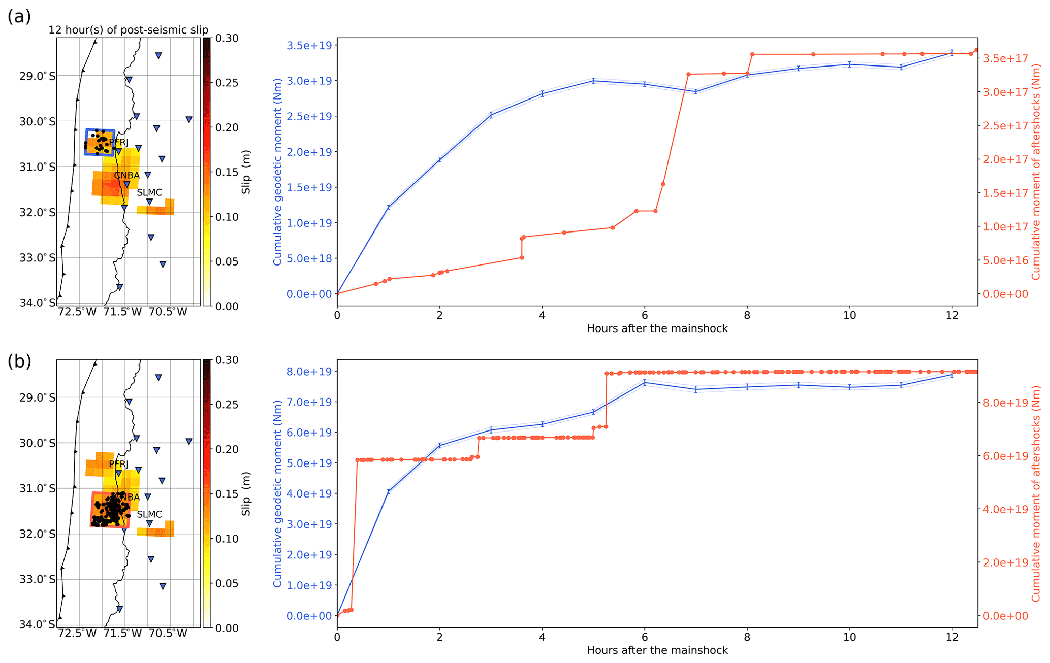
Figure 6(a) On the left, we show a map highlighting the region considered for the calculations (blue square) that we define as the northern patch in the main text. On the right, we show the time evolution of the geodetic moment (blue curve) along with the time evolution of the seismic moment from the aftershocks (red curve). (b) On the left, we show a map outlining the region considered for the calculations (red square) that we define as the southern patch in the main text. On the right, we show the time evolution of the geodetic moment (blue curve) along with the time evolution of the seismic moment from the aftershocks (red curve).
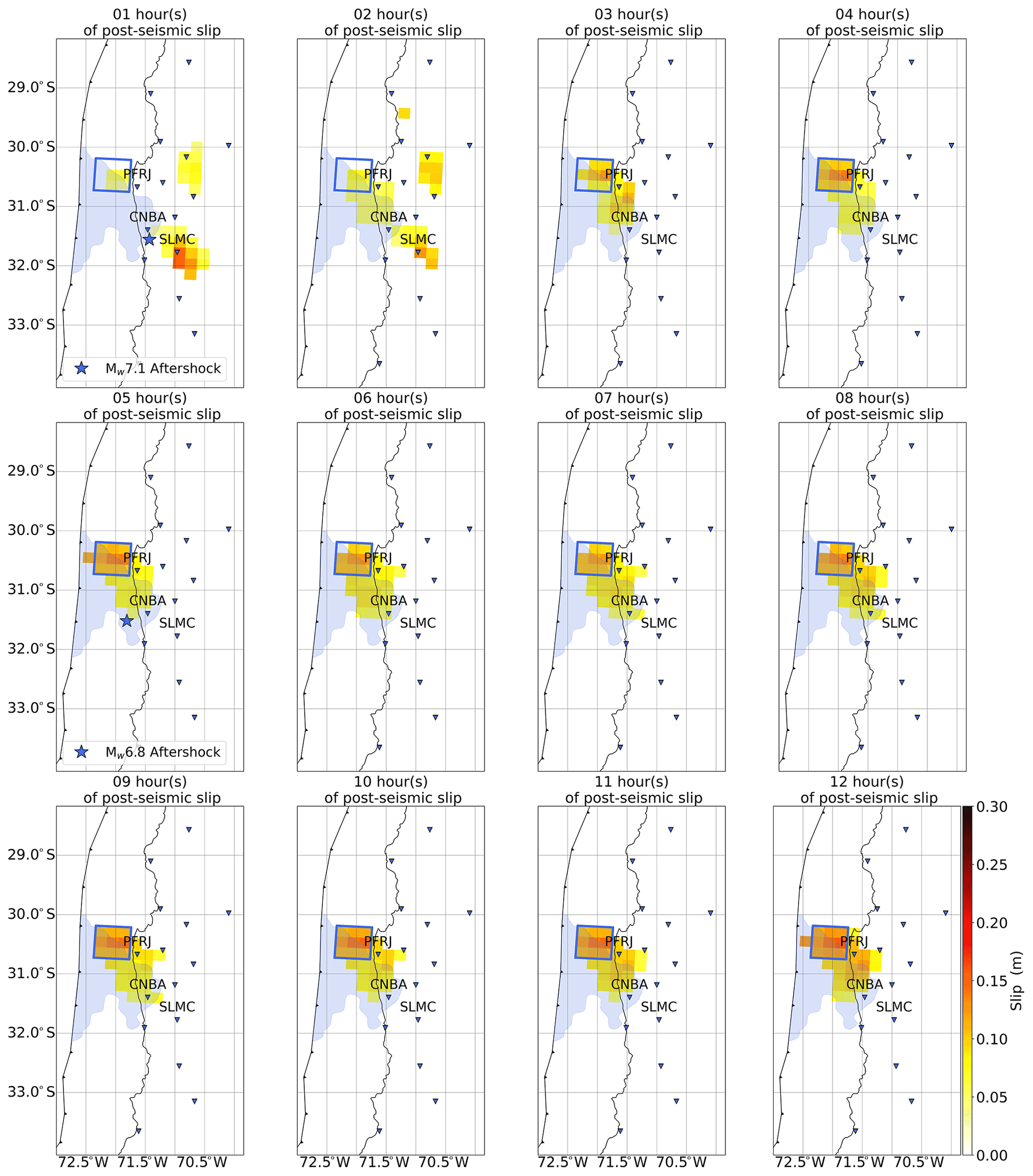
Figure 7This is the same as Fig. 3 except that these hourly images have been obtained after removing the two largest aftershocks from the position time series. The blue square outlines what we refer to as the northern patch.
Hence, to better isolate aseismic slip, we use corrected position time series, of which the contribution of the two largest aftershocks is removed, to obtain hourly images of the post-seismic slip. The results can be seen in Fig. 7. Our models show that post-seismic slip is now only observed north of the co-seismic rupture area and that the patch to the south has completely vanished. Therefore, it supports even further the fact that post-seismic slip south of the mainshock rupture area is likely the result of seismic slip only from the aftershocks. On the contrary, post-seismic slip to the north is likely aseismic as the contribution of aftershocks (3.5 × 10¹⁷ Nm) is small compared to the geodetic moment of this patch (1.7 × 10¹⁹ Nm). We note that the geodetic moment of the northern patch remains similar to the previous estimate obtained using the non-corrected position time series. This illustrates that this patch is stable, regardless of the dataset used.
As a next step, we analyze the temporal evolution between the amount of aseismic afterslip and the number of aftershocks in the northern patch (Fig. 8, and Supplement S7 for the same comparison using the catalog of Frank et al., 2017). First, we find that the cumulative afterslip exhibits a logarithmic trend. Similarly to other studies carried out in Ecuador and Japan (Tsang et al., 2019; Milliner et al., 2020, respectively), we do not observe the acceleration phase of afterslip predicted by Perfettini and Ampuero (2008). Indeed, before reaching the steady state, under a rate-and-state friction law, slip is expected to accelerate transiently before it starts to expand quasi-statically. Thus, our results suggest that for this earthquake also, the steady state is reached very quickly after the mainshock (< 1 h). When we make the comparison with the cumulative number of aftershocks, we find that the two curves do not follow the same trend. This seems at odds with observations made on the early times of the post-seismic phase by Tsang et al. (2019) and Milliner et al. (2020). As these two studies do not specifically focus on the first 12 h but rather on the trend over a couple of days, it would be very interesting to investigate in detail what happens during the very early stage of the post-seismic phase for these two examples.
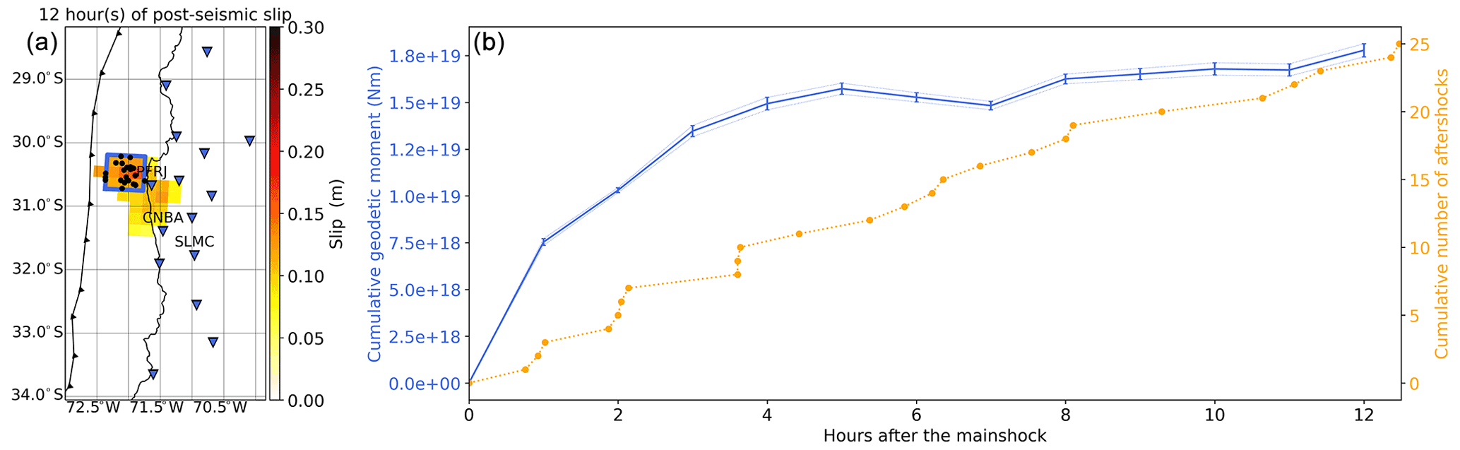
Figure 8(a) Post-seismic slip distribution after 12 h and obtained using the position time series with the two largest aftershocks removed. We show with the blue square the identified northern patch that is slipping almost purely aseismically. The black dots show the aftershocks inside this region from the catalog of Huang et al. (2017). See Fig. 1 for details on the symbols. (b) Time evolution of the cumulative geodetic moment of afterslip (blue line) along with the time evolution of the cumulative number of aftershocks (orange dotted line). All curves are obtained from the inside of the blue rectangle shown on (a).
Based on theoretical arguments, Perfettini and Avouac (2004) suggest that if afterslip is driving the generation of aftershocks, we should expect a similar time evolution between the cumulative number of aftershocks and the cumulative afterslip. Their analysis assumes that the deformation from aftershocks should be small compared to that of afterslip and that steady state is reached, and both criteria seem to be met here. But the fact that we do not observe such a relationship is not incompatible with the fact that afterslip drives aftershocks even just after the mainshock. For instance, following the Parkfield Earthquake in California, Savage (2007) showed that there could be a deviation from that expected relationship, especially at the beginning of the post-seismic sequence, even when hypothesizing that afterslip drives aftershocks. The way aftershocks respond to stress changes may be quite complex, especially when considering the full rate-and-state friction law (e.g., Dieterich, 1994; Kaneko and Lapusta, 2008; Helmstetter and Shaw, 2009). It is also possible that very early aftershocks are triggered by the mainshock static stress changes and that it is only later that afterslip starts to drive aftershocks (Perfettini et al., 2018a). Other processes could also be candidates as the driving mechanism for aftershock generation (e.g., fluid flow, Miller, 2020). We also cannot rule out the fact that the earthquake catalog might still be incomplete, thus missing aftershocks at the very early stage of the post-seismic phase.
To summarize, we find here that post-seismic slip can arise from distinct frictional properties on the fault. To the south, slip is essentially seismic, which can be usually associated with a velocity-weakening regime under the rate-and-state friction law framework. Instead, to the north, slip is almost purely aseismic, which is more in line with a velocity-strengthening regime. We can hypothesize regarding the causes of that bimodal behavior. For instance, Poli et al. (2017) suggest that fracture zones enclose the mainshock rupture area favoring fluids circulation at these places. Differences in the pore-fluid pressure between the north and the south could be why we observe distinct behaviors. The nature of the plate interface could also be invoked to explain the bimodal behavior of afterslip. For instance, Comte et al. (2019) provide evidence of strong lithological contrast at the region of the Illapel earthquake, likely explained by materials being dragged down by the erosive Chilean margin. This could generate high variability of the plate interface roughness. Lange et al. (2016) also propose that plate interface rugosity plays a role in controlling the spatial pattern of longer-term Illapel's aftershocks (the first 24 h). Thus, roughness of the plate interface could explain the heterogeneity of the slip modes in this area. We also find that the southern patch is associated with a high coupling of the plate interface while the one to the north is at a transition zone between high and low coupling (Métois et al., 2014). This could explain why one region favors seismic slip (south) while the other favors aseismic slip (north). Still, the fact that we can very early on suggest that the fault is divided into regions of distinct frictional properties can prove to be useful for forecast the spatial pattern of aftershocks.
4.2 Potential to use very early post-seismic data to forecast aftershock location
Most of the physics-based models of aftershock sequences used for forecasting do not include information about post-seismic slip, although the study by Cattania et al. (2015) shows that it could have a positive impact on the forecast.
In the case of the Illapel earthquake, we show that the surface observations carry enough information to image the spatiotemporal evolution of post-seismic slip very early after the mainshock. We also see that the slip pattern inferred at this very early stage does not evolve much over time. This is not an isolated example as Tsang et al. (2019) made a similar inference for the 2016 Pedernales, Ecuador, earthquake, with the slip patches imaged over the first 72 h persisting after 30 d. Milliner et al. (2020) provides another example of such behavior following the 2016 Kumamoto, Japan, earthquake. Thus, post-seismic slip from the first hours after the mainshock can help characterize longer-lasting post-seismic slip. Finally, we also show that differences in frictional behavior can be revealed from the very first stage of the post-seismic phase. Thus, imaging the very early post-seismic slip with little time latency could provide valuable additional information to help forecasting the spatial pattern of aftershocks.
Getting images of the slip distribution is not the main challenge as the problem is linear and computationally rather fast. The challenge lies more in the ability to obtain GNSS position time series rapidly with a low-enough noise level. Thanks to the growing number of GNSS networks worldwide, along with the improvement of the processing techniques, we find an increasing number of examples showing that it is possible to accurately monitor in near-real-time various geophysical processes, whether these processes involve seismic slip and/or aseismic slip. For instance, such monitoring is done for the rapid study of earthquakes (e.g., Murray et al., 2018; Melgar et al., 2019), or to monitor volcanic activities (e.g., Neal et al., 2019), but with an accuracy of only a few centimeters.
To the best of our knowledge, the Nevada Geodetic Laboratory (NGL) has provided open access since 2019 to 5 min position time series with a 1 h latency (so-called ultra-rapid solutions), and for a significant number of GNSS stations worldwide (see Blewitt et al., 2018, for details about the data available at the NGL). However, the short latency at which these solutions are made available is associated with an increase in the noise level compared to the solution used in this study. Therefore, we first have to assess if the noise level of these observations is low enough to infer information about the very early post-seismic slip.
Thus, we compare the noise level of the position time series from the two stations of our study which are also available from the NGL, CERN, and SANT. We choose the period of July 2019 as there are no significant earthquakes reported nearby in the GCMT catalog. The average standard deviation of the ultra-rapid NGL time series is 0.95 and 1.31 cm for the east and north components, respectively, which is higher than for the post-processed time series used in this study (0.26 and 0.30 cm for the east and north components, respectively). But we note that 5 out of 15 stations that we use show surface displacements that are larger than 1.31 cm after just 1 h. Thus, given the 1 h latency before the NGL ultra-rapid position time series are made available, it would have been possible to obtain an image of the first hour of the post-seismic slip ∼ 2 h after the occurrence of the mainshock. This preliminary conclusion is promising in the prospect of including information about very early post-seismic slip for the forecasting of aftershock locations. Of course, some tests will be necessary to assess the impact of adding such information for the forecast of aftershocks and to evaluate whether or not this could ever be implemented operationally.
Over the first 12 h following the 2015 Mw 8.3 Illapel earthquake, we find that very early post-seismic slip develops essentially over two regions located on the edges of the co-seismic rupture area. When compared to the spatiotemporal evolution of the very early aftershocks, we find a good spatial correlation. However, the underlying physics driving the slip in these two regions is different. To the south, we show that post-seismic slip is purely seismic and caused by the occurrence of aftershocks. Once we account for the two largest ones, slip in this region vanishes. To the north, we find that post-seismic slip is almost purely aseismic. Our findings show that in this region, afterslip does not exhibit the acceleration phase predicted from theory suggesting a rather fast transition from co-seismic to steady-state post-seismic slip (< 1 h). As to whether or not very early afterslip is the driving mechanism of very early aftershocks, we cannot provide a clear answer. Indeed, we obtain an unusual relationship between the time evolution of afterslip and the cumulative number of aftershocks. However, this might not be incompatible with the fact that afterslip drives aftershocks based on the study by Savage (2007). At the same time, other hypotheses can also be proposed to explain this unusual observation (e.g., delay in the role played by afterslip, influence of fluid flow, etc.). Observations of the very early post-seismic phase, at high temporal resolution, could thus be crucial to discriminate between these competing processes.
Our additional finding is that the slip patterns that we observe after 12 h persist over the first 2 months. While it is currently difficult to predict whether or not the very early post-seismic slip pattern will always be informative about long-term afterslip patterns, the increasing number of studies on that very early phase should help clarify that question. Thus, in the case when information about very early post-seismic slip helps to characterize longer-lasting post-seismic slip, it could be useful to include it for the forecast of aftershock locations. In this perspective, we suggest that an image of the first hour after seismic activity could be obtained within ∼ 2 h after the mainshock origin time when using ultra-rapid position time series such as those computed at the NGL. Thus, future studies could test our capacity to image very early post-seismic slip in near-real time and investigate what this new piece of information could bring for the forecasting of the spatial distribution of aftershocks.
The 30 s kinematic position time series used in this study can be found here: https://github.com/cedrictwardz/2015_IllapelEarthquake_PositionTimeSeries.git (Twardzik, 2021a). A Python code used for building and applying the sidereal filter to the raw position time series can be found here: https://github.com/cedrictwardz/SiderealFilter.git (Twardzik, 2021b).
The supplement related to this article is available online at: https://doi.org/10.5194/se-12-2523-2021-supplement.
CT processed the GNSS data, performed the post-seismic slip inversion, and wrote the paper with inputs from all co-authors.
The authors declare that they have no conflict of interest.
Publisher’s note: Copernicus Publications remains neutral with regard to jurisdictional claims in published maps and institutional affiliations.
The continuous GNSS stations are part of the Chilean GNSS network maintained by the Centro Sismológico Nacional of the University of Chile (Baez et al., 2018). We thank Christophe Vigny for facilitating the access to the GNSS data. We thank the editorial team and Bernd Schurr, Mathilde Radiguet, and one anonymous referee as well as the community reviewer Dietrich Lange. All the comments and suggestions have greatly improved the quality of the work presented here.
This research has been supported by the Agence Nationale de la Recherche (grant no. ANR 14-CE03-0002-01JCJC E-POST), the European Research Council, H2020 European Research Council (grant no. PRESEISMIC (805256)), and the Centre National d'Etudes Spatiales.
This paper was edited by CharLotte Krawczyk and reviewed by Bernd Schurr, Mathilde Radiguet, and one anonymous referee.
Baez, J. C., Leyton, F., Troncoso, C., del Campo, F., Bevis, M., Vigny, C., Moreno, M., Simons, M., Kendrick, E., Parra, H., and Blume, F.: The Chilean GNSS Network: Current Status and Progress toward Early Warning Applications, Seism. Res. Lett., 89, 1546–1554, https://doi.org/10.1785/0220180011, 2018. a, b
Barnhart, W. D., Murray, J. R., Biggs, R. W., Gomez, F., Miles, C. P. J., Svarc, J., Riquelme, S., and Stressler, B. J.: Coseismic slip and early afterslip of the 2015 Illapel, Chile, earthquake: Implications for frictional heterogeneity and coastal uplift, J. Geophys. Res.-Sol. Ea., 121, 6172–6191, https://doi.org/10.1002/2016JB013124, 2016. a, b
Bedford, J., Moreno, M., Baez, J., Lange, D., Tilmann, F., Rosenau, M., Heidbach, O., Oncken, O., Bartsch, M., Rietbrock, A., Tassara, A., Bevis, M., and Vigny, C.: A high-resolution, time-variable afterslip model for the 2010 Maule Mw=8.8, Chile megathrust earthquake, Earth Planet. Sc. Lett., 383, 26–36, https://doi.org/10.1016/j.epsl.2013.09.020, 2013. a
Bilek, S. L. and Lay, T.: Subduction zone megathrust earthquakes, Nature, 400, 443–446, https://doi.org/10.1038/22739, 1999. a
Bird, P.: An updated digital model of plate boundaries, Geochem. Geophy. Geosy., 4, 1027, https://doi.org/10.1029/2001GC000252, 2003. a
Blewitt, G., Hammond, W. C., and Kreemer, C.: Harnessing the GPS data explosion for interdisciplinary science, EOS, 99, https://doi.org/10.1029/2018EO104623, 2018. a
Carrasco, S., Ruiz, J. A., Contreras-Reyes, E., and Ortega-Culaciati, F.: Shallow intraplate seismicity related to the Illapel 2015 Mw 8.4 earthquake: Implications from the seismic source, Tectonophysics, 766, 205–218, https://doi.org/10.1016/j.tecto.2019.06.011, 2019. a
Cattania, C., Hainzl, S., Wang, L., Enescu, B., and Roth, R.: Aftershocks triggering by postseismic stresses: A study based on Coulomb rate-and-state models, J. Geophys. Res., 120, 2388–2407, https://doi.org/10.1002/2014JB011500, 2015. a
Choi, K.: Improvements in GPS precision: 10 Hz to one day, Ph.D. thesis, Department of Aerospace Engineering Sciences, University of Colorado, Boulder, Colorado, USA, 2007. a, b
Colletini, C., Niemeijer, A., Viti, C., Smith, S. A. F., and Marone, C.: Fault structure, frictional properties and mixed-mode fault slip behavior, Earth Planet. Sc. Lett., 311, 316–327, 2011. a
Comte, D., Farias, M., Roecker, S., and Russo, R.: The nature of the subduction wedge in an erosive margin: Insights from the analysis of aftershocks of the 2015 Mw 8.3 Illapel earthquake beneath the Chilean Coastal Range, Earth Planet. Sc. Lett., 520, 50–62, https://doi.org/10.1016/j.epsl.2019.05.033, 2019. a
Das, S. and Henry, C.: Spatial relation between main earthquake slip and its aftershock distribution, Rev. Geophys., 43, 1013, https://doi.org/10.1029/2002RG000119, 2003. a
Das, S. and Scholz, C. H.: Off-fault aftershock clusters caused by shear-stress increase?, Bull. Seism. Soc. Am., 71, 1669–1675, 1981. a
Dasher-Cousineau, K., Brodsky, E. E., Lay, T., and Goebel, T. H. W.: What controls variations in aftershock productivity?, J. Geophys. Res.-Sol. Ea., 125, e2019JB018111, https://doi.org/10.1029/2019JB018111, 2020. a
DeMets, C., Gordon, R. G., and Argus, D. F.: Geologically current plate motions, Geophys. J. Int., 181, 1–80, https://doi.org/10.1111/j.1365-246X.2009.04491.x, 2012. a
Dieterich, J.: A constitutive law for rate of earthquake production and its application to earthquake clustering, Geophys. J. Int., 99, 2601–2618, https://doi.org/10.1029/93JB02581, 1994. a
Ekström, G., Nettles, M., and Dziewonski, A.: The global CMT project 2004-2010: Centroid-moment tensors for 13 017 earthquakes, Phys. Earth Planet. Int., 200/201, 1–9, https://doi.org/10.1016/j.pepi.2012.04.002, 2012. a
Feng, W., Samsonov, S., Tian, Y., Qiu, Q., Li, P., Zhang, Y., Deng, Z., and Omari, K.: Surface deformation associated with the 2015 Mw 8.3 Illapel earthquake revealed by satellite-based geodetic observations and its implications for the seismic cycle, Earth Planet. Sc. Lett., 460, 222–233, https://doi.org/10.1016/j.epsl.2016.11.018, 2017. a
Frank, W. B., Poli, P., and Perfettini, H.: Mapping the rheology of central Chile subduction zone with aftershocks, Geophys. Res. Lett., 44, 5374—5382, https://doi.org/10.1002/2016GL072288, 2017. a, b, c
Guo, R., Zheng, Y., Xu, J., and Riaz, M. S.: Transient viscosity and afterslip of the 2015 Mw 8.3 Illapel, Chile, earthquake, Bull. Seism. Soc. Am., 109, 2567–2581, https://doi.org/10.1785/0120190114, 2019. a
Hainzl, S.: Apparent triggering function of aftershocks resulting from rate-dependent incompleteness of earthquake catalogs, J. Geophys. Res.-Sol. Ea., 121, 6499–6509, https://doi.org/10.1002/2016JB013319, 2016. a
Hayes, G. P., Wald, D. J., and Johnson, R. L.: Slab1.0: A three-dimensional model of global subduction zone geometries, J. Geophys. Res.-Sol. Ea., 117, B01302, https://doi.org/10.1029/2011JB008524, 2012. a
Heki, K. and Tamura, Y.: Short term afterslip in the 1994 Sanriku-Haruka-Oki earthquake, Geophys. Res. Lett., 24, 3285–3288, https://doi.org/10.1029/97GL03316, 1997. a
Helmstetter, A. and Shaw, B. E.: Afterslip and aftershocks in the rate-and-state friction law, J. Geophys. Res.-Sol. Ea., 114, B01308, https://doi.org/10.1029/2007JB005077, 2009. a, b
Huang, H., Xu, W., Meng, L., BB̈urgmann, R., and Baez, J. C.: Early aftershocks and afterslip surrounding the 2015 Mw 8.4 Illapel rupture, Earth Planet. Sc. Lett., 457, 282—291, https://doi.org/10.1016/j.epsl.2016.09.055, 2017. a, b, c, d, e
Jiang, J., Bock, Y., and Klein, E.: Coevolving early afterslip and aftershock signatures of a San Andreas fault rupture, Sci. Adv., 7, eabc1606, https://doi.org/10.1126/sciadv.abc1606, 2021. a, b
Kaneko, Y. and Lapusta, N.: Variability of earthquake nucleation in continuum models of rate-and-state faults and implications for aftershock rates, J. Geophys. Res., 113, B12312, https://doi.org/10.1029/2007JB005154, 2008. a
Kirb, D., Gomberg, J., and Bodin, P.: Aftershock triggering by complete Coulomb stress changes, J. Geophys. Res.-Sol. Ea., 107, ESE 2-1–ESE 2-14, https://doi.org/10.1029/2001JB000202, 2002. a
Klein, E., Vigny, C., Fleitout, L., Grandin, R., Jolivet, R., Rivera, E., and Metois, M.: A comprehensive analysis of the Illapel 2015 Mw 8.3 earthquake from GPS and InSAR data, Earth Planet. Sc. Lett., 469, 123–134, https://doi.org/10.1016/j.epsl.2017.04.010, 2017. a
Konca, A., Hjorleifsdottir, V., Song, T.-R., Avouac, J.-P., Helmberger, D., Ji, C., Sieh, K., Briggs, R., and Meltzner, A.: Rupture Kinematics of the 2005 Mw8.6 Nias–Simeulue Earthquake from the Joint Inversion of Seismic and Geodetic Data, Bull. Seism. Soc. Am., 97, S307–S322, https://doi.org/10.1785/0120050632, 2007. a
Langbein, J., Murray, J. R., and Snyder, H. A.: Coseismic and initial postseismic deformation from the 2004 Parkfield, California, earthquake, observed by Global Positioning System, electronic distance meter, creepmeters, and borehole strainmeters, Bull. Seism. Soc. Am., 96, S304–S320, 2006. a
Lange, D., Bedford, J. R., Moreno, M., Tilmann, F., Baez, J. C., Bevis, M., and Krüger, F.: Comparison of postseismic afterslip models with aftershock seismicity for three subduction-zone earthquakes: Nias 2005, Maule 2010 and Tohoku 2011, Geophys. J. Int., 199, 784–799, https://doi.org/10.1093/gji/ggu292, 2014. a
Lange, D., Geersen, J., Barrientos, S., Moreno, M., Grevemeyer, I., Contreras-Reyes, E., and Kopp, H.: Aftershock seismicity and tectonic setting of the 2015 September 16 Mw 8.3 Illapel earthquake, Central Chile, Geophys. J. Int., 206, 1424–1430, https://doi.org/10.1093/gji/ggw218, 2016. a
Laske, G., Masters, G., Ma, Z., and Pasyanos, M.: Update on CRUST1.0 – A 1-degree global model of Earth's crust, Geophys. Res. Abstracts, 15, Abstract EGU2013–2658, 2013. a
Mallman, E. P. and Zoback, M. D.: Assessing elastic Coulomb stress transfer models using seismicity rates in southern California and southwestern Japan, J. Geophys. Res.-Sol. Ea., 112, B03304, https://doi.org/10.1029/2005JB004076, 2007. a
Malservisi, R., S. Y. Schwartz, N. V., Protti, M., Gonzalez, V., Dixon, T. H., Jiang, Y., Newmann, A. V., Richardson, J., Walter, J. I., and Voyanko, D.: Multiscale postseismic behavior on a megathrust: The 2012 Nicoya earthquake, Costa Rica, Geochem. Geophy. Geosy., 16, 1848–1864, https://doi.org/10.1002/2015GC005794, 2015. a
Marone, C. J., Scholtz, C. H., and Bilham, R.: On the mechanics of earthquake afterslip, J. Geophys. Res., 96, 8441–8452, https://doi.org/10.1029/91JB00275, 1991. a
Meade, B. J., DeVries, P. M. R., Faller, J., Viegas, F., and Wattenberg, M.: What Is Better Than Coulomb Failure Stress? A Ranking of Scalar Static Stress Triggering Mechanisms from 105 Mainshock-Aftershock Pairs, Geophys. Res. Lett., 44, 11409–11416, https://doi.org/10.1002/2017GL075875, 2017. a
Melgar, D., Fan, W., Riquelme, S., Geng, J., Liang, C., Fuentes, M., Vargas, G., Allen, R. M., Shearer, P. M., and Fielding, E.: Slip segmentation and slow rupture to the trench during the 2015 Mw 8.3 Illapel, Chile, earthquake, Geophys. Res. Lett., 43, 961–966, https://doi.org/10.1002/2015GL067369, 2016. a, b
Melgar, D., Melbourne, T. I., Crowell, B. W., Geng, J., Szeliga, W., Scrivner, C., Santillan, M., and Goldberg, D. E.: Real-time high-rate GNSS displacements: Performance demonstration during the 2019 Ridgecrest, California, earthquake, Seism. Res. Lett., 91, 1943–1951, https://doi.org/10.1785/0220190223, 2019. a
Métois, M., Vigny, C., Socquet, A., Delorme, A., Morvan, S., Ortega, I., and Valderas-Bermejo, C.-M.: GPS-derived interseismic coupling on the subduction and seismic hazards in the Atacama region, Chile, Geophys. J. Int., 196, 644–655, https://doi.org/10.1093/gji/ggt418, 2014. a
Mignan, A.: Modeling aftershocks as a stretched exponential relaxation, Geophys. Res. Lett., 42, 9726–9732, https://doi.org/10.1002/2015GL066232, 2015. a
Miller, S. A.: Aftershocks are fluid-driven and decay rates controlled by permeability dynamics, Nat. Commun., 11, 5787, https://doi.org/10.1038/s41467-020-19590-3, 2020. a, b
Milliner, C., Bürgmann, R., Inbal, A., Wang, T., and Liang, C.: Resolving the Kinematics and Moment Release of Early Afterslip Within the First Hours Following the 2016 Mw 7.1 Kumamoto Earthquake: Implications for the Shallow Slip Deficit and Frictional Behavior of Aseismic Creep, J. Geophys. Res.-Sol. Ea., 125, e2019JB018928, https://doi.org/10.1029/2019JB018928, 2020. a, b, c, d
Miyazaki, S. and Larson, K.: Coseismic and early postseismic slip for the 2003 Tokachioki earthquake sequence inferred from GPS data, Geophys. Res. Lett., 35, L04302, https://doi.org/10.1029/2007GL032309, 2008. a, b
Munekane, H.: Coseismic and early postseismic slips associated with the 2011 off the Pacific coast of Tohoku Earthquake sequence: EOF analysis of GPS kinematic time series, Earth Planet. Space, 64, 3, https://doi.org/10.5047/eps.2012.07.009, 2012. a
Murray, J. R., Crowell, B. W., Grapenthin, R., Hodgkinson, K., Langbein, J. O., Melbourne, T., Melgar, D., Minson, S. E., and Schmidt, D. A.: Development of a geodetic component for the U.S. West Coast earthquake early warning system, Seism. Res. Lett., 89, 2322–2336, https://doi.org/10.1785/0220180162, 2018. a
Neal, C. A., Brantley, S. R., Antolik, L., Babb, J. L., Burgess, M., Calles, K., Cappos, M., Chang, J. C., Conway, S., Desmither, L., Dotray, P., Elias, T., Fukunaga, P., Fuke, S., Johansen, I. A., Kamibayashi, K., Kauahikaua, J., Lee, R. L., Pekalib, S., Miklius, A., Millon, W., Moniz, C. J., Nadeau, P. A., Okubo, P., Parcheta, C., Patrick, M. R., Shiro, B., Swanson, D. A., Tollett, W., Trusdell, F., Younger, E. F., Zoeller, M. H., Montgomery-Brown, E. K., Anderson, K. R., Poland, M. P., Ball, J. L., Bard, J., Coombs, M., Dietterich, H. R., Kern, C., Thelen, W. A., Cervelli, P. F., Orr, T., Houghton, B. F., Gansecki, C., Hazlett, R., Lundgren, P., Diefenbach, A. K., Lerner, A. H., Waite, G., Kelly, P., Clor, L., Werner, C., Mulliken, K., Fisher, G., and Damby, D.: The 2018 rift eruption and summit collapse of Kilauea volcano, Science, 363, 367–374, https://doi.org/10.1126/science.aav7046, 2019. a
Okada, Y.: Surface deformation due to shear and tensile faults in a half-space, Bull. Seism. Soc. Am., 75, 1135–1154, 1985. a
Omori, F.: On the after-shocks of earthquakes, J. Sc. Coll., 7, 111–120, 1894. a
Ozawa, S. and Ando, R.: Mainshock and Aftershock Sequence Simulation in Geometrically Complex Fault Zones, J. Geophys. Res.-Sol. Ea., 126, e2020JB020865, https://doi.org/10.1029/2020JB020865, 2021. a
Peng, Z. and Zhao, P.: Migration of early aftershocks following the 2004 Parkfield earthquake, Nat. Geosci., 2, 877–881, https://doi.org/10.1038/ngeo697, 2009. a
Perfettini, H. and Ampuero, J.-P.: Dynamics of a velocity strengthening fault region: Implications for slow earthquakes and postseismic slip, J. Geophys. Res.-Sol. Ea., 113, B09411, https://doi.org/10.1029/2007JB005398, 2008. a
Perfettini, H. and Avouac, J. P.: Postseismic relaxation driven by brittle creep: A possible mechanism to reconcile geodetic measurements and the decay rate of aftershocks, application to the Chi-Chi earthquake, Taiwan, J. Geophys. Res.-Sol. Ea., 109, B02304, https://doi.org/10.1029/2003JB002488, 2004. a
Perfettini, H. and Avouac, J. P.: Modeling afterslip and aftershocks following the 1992 Landers earthquake, J. Geophys. Res.-Sol. Ea., 112, B07409, https://doi.org/10.1029/2006JB004399, 2007. a
Perfettini, H., Frank, W. B., Marsan, D., and Bouchon, M.: A Model of Aftershock Migration Driven by Afterslip, Geophys. Res. Lett., 45, 2283–2293, https://doi.org/10.1002/2017GL076287, 2018a. a
Perfettini, H., Frank, W. B., Marsan, D., and Bouchon, M.: A Model of Aftershock Migration Driven by Afterslip, Geophys. Res. Lett., 45, 2283–2293, https://doi.org/10.1002/2017GL076287, 2018b. a
Perfettini, H., Frank, W. B., Marsan, D., and Bouchon, M.: Updip and Along-Strike Aftershock Migration Model Driven by Afterslip: Application to the 2011 Tohoku-Oki Aftershock Sequence, J. Geophys. Res.-Sol. Ea., 124, 2653—2669, https://doi.org/10.1029/2018JB016490, 2019. a
Pianatesi, A., Cirella, A., Spudich, P., and Cocco, M.: A global search inversion for earthquake kinematic rupture history: Application to the 2000 western Tottori, Japan, earthquake, J. Geophys. Res.-Sol. Ea., 112, B07314, https://doi.org/10.1029/2006JB004821, 2007. a, b, c
Poli, P., Maksymowicz, A., and Ruiz, S.: The Mw8.3 Illapel earthquake (Chile): Preseismic and postseismic activity associated with hydrated slab structures, Geology, 45, 247–250, https://doi.org/10.1130/G38522.1, 2017. a
Romanet, P., Bhat, H. S., Jolivet, R., and Madariaga, R.: Fast and slow slip events emerge due to fault geometrical complexity, Geophys. Res. Lett., 45, 4809–4819, https://doi.org/10.1029/2018GL077579, 2018. a
Ross, Z. E., Rollins, C., Cochran, E. S., Hauksson, E., Avouac, J. P., and Ben-Zion, Y.: Aftershocks driven by afterslip and fluid pressure sweeping through a fault-fracture mesh, Geophys. Res. Lett., 44, 8260–8267, https://doi.org/10.1002/2017GL074634, 2017. a
Ruiz, S., Klein, E., del Campo, F., Rivera, E., Poli, P., Metois, M., Vigny, C., Baez, J. C., Vargas, G., Leyton, F., Madariaga, R., and Fleitout, L.: The Seismic Sequence of the 16 September 2015 Mw 8.3 Illapel, Chile, Earthquake, Seism. Res. Lett., 87, 789–799, https://doi.org/10.1785/0220150281, 2016. a
Salman, R., Hill, E., Feng, L., Lindsey, E., Veedu, D. M., Barbot, S., Banerjee, P., Hermawan, I., and Natawidjaja, D.: Piecemeal rupture of the Mentawai Patch, Sumatra: the 2008 Mw 7.2 North Pagai earthquake sequence, J. Geophys. Res.-Sol. Ea., 122, 9404–9419, https://doi.org/10.1002/2017JB014341, 2017. a
Savage, J.: Calculation of aftershock accumulation from observed postseismic deformation: M6 2004 Parkfield, California, earthquake, Geophys. Res. Lett., 37, L13302, https://doi.org/10.1029/2010GL042872, 2007. a
Schurr, B., Asch, G., Hainzl, S., Bedford, J., Hoechner, A., Palo, M., Wang, R., Moreno, M., Bartsch, M., Zhang, Y., Oncken, O., Tilmann, F., Dahm, T., Victor, P., Barrientos, S., and Vilotte, J. P.: Gradual unlocking of plate boundary controlled initiation of the 2014 Iquique earthquake, Nature, 512, 299–302, https://doi.org/10.1038/nature13681, 2014. a
Sen, M. K. and Stoffa, P. L.: Global optimization methods in geophysical inversion, 2nd Edn., Cambridge University Press, Cambridge, United Kingdom, 2013. a
Shelly, D. R.: A High-Resolution Seismic Catalog for the Initial 2019 Ridgecrest Earthquake Sequence: Foreshocks, Aftershocks, and Faulting Complexity, Seism. Res. Lett., 91, 1971–1978, https://doi.org/10.1785/0220190309, 2020. a
Shrivastava, M. N., Gonzalez, G., Moreno, M., Chlieh, M., Salazar, P., Reddy, C. D., Baez, J. C., nez, G. Y., Gonzalez, J., and de la Llera, J. C.: Coseismic slip and afterslip of the 2015 Mw 8.3 Illapel (Chile) earthquake determined from continous GPS data, Geophys. Res. Lett., 43, 10710–10719, https://doi.org/10.1002/2016GL070684, 2016. a
Thingbaijam, K. K. S., Mai, P. M., and Goda, K.: New empirical earthquake source-scaling laws, Bull. Seism. Soc. Am., 107, 2225–2246, https://doi.org/10.1785/0120170017, 2017. a
Tsang, L. L. H., Vergnolle, M., Twardzik, C., Sladen, A., Nocquet, J. M., Rolandone, F., Agurto-Detzel, H., Cavalié, O., Jarrin, P., and Mothes, P.: Imaging rapid early afterslip of the 2016 Pedernales earthquake, Ecuador, Earth Planet. Sc. Lett., 524, 115724, https://doi.org/10.1016/j.epsl.2019.115724, 2019. a, b, c, d
Twardzik, C.: 30s Position Time Series for the 2015 Illapel earthquake, Zenodo [data set], https://doi.org/10.5281/zenodo.5636139, 2021a.
Twardzik, C.: Python Code for sidereal filtering, Zenodo [code], https://doi.org/10.5281/zenodo.4498160, 2021b.
Twardzik, C., Vergnolle, M., Sladen, A., and Avallone, A.: Unravelling the contribution of early postseismic deformation using sub-daily GNSS positioning, Sci. Rep., 9, 1775, https://doi.org/10.1038/s41598-019-39038-z, 2019. a, b, c, d, e
Utsu, T. and Seki, A.: A relation between the area of aftershock region and the energy of the main shock, J. Seism. Soc. Jpn., 7, 233–240, 1954. a
Utsu, T., Ogata, Y., and Matsu'ura, R.: The centenary of the Omori formula for a decay law of aftershock activity, J. Phys. Earth, 43, 1–33, https://doi.org/10.4294/jpe1952.43.1, 1995. a
van der Elst, N. J. and Shaw, B. E.: Larger aftershocks happen farther away: Nonseparability of magnitude and spatial distributions of aftershocks, Geophys. Res. Lett., 42, 5771–5778, https://doi.org/10.1002/2015GL064734, 2015. a
Wang, X., Wei, S., and Wu, W.: Double-ramp on the Main Himalayan Thrust revealed by broadband waveform modeling of the 2015 Gorkha earthquake sequence, Earth Planet. Sc. Lett., 473, 83–93, https://doi.org/10.1016/j.epsl.2017.05.032, 2017. a
Wetzler, N., Lay, T., Brodsky, E. E., and Kanamori, H.: Systematic deficiency of aftershocks in areas of high coseismic slip for large subduction zone earthquakes, Sci. Adv., 4, eaao3225, https://doi.org/10.1126/sciadv.aao3225, 2018. a
Zhu, L. and Rivera, L.: A note on the dynamic and static displacements from a point source in multilayered media, Geophys. J. Int., 148, 619–627, https://doi.org/10.1046/j.1365-246X.2002.01610.x, 2002. a