Multi-array analysis of volcano-seismic signals at Fogo and Brava, Cape Verde

Seismic arrays provide tools for the localization of events without clear phases or events outside the network, where the station coverage prohibits classical localization techniques. Beam forming allows the determination of the direction (back azimuth) and horizontal (apparent) velocity of an incoming wavefront. Here we combine multiple arrays to retrieve event epicentres from the area of intersecting beams without the need to specify a velocity model. The analysis is performed in the time domain, which allows selecting a relatively narrow time window around the phase of interest while preserving frequency bandwidth. This technique is applied to earthquakes and hybrid events in the region of Fogo and Brava, two islands of the southern chain of the Cape Verde archipelago. The results show that the earthquakes mainly originate near Brava, whereas the hybrid events are located on Fogo. By multiple-event beam stacking we are able to further constrain the epicentral locations of the hybrid events in the northwestern part of the collapse scar of Fogo. In previous studies, these events were attributed to shallow hydrothermal processes. However, we obtain relatively high apparent velocities at the arrays, pointing to either deeper sources or complex ray paths. For a better understanding of possible errors of the multi-array analysis, we also compare slowness values obtained from the array analysis with those derived from earthquake locations from classical (local network) localizations. In general, the results agree well. Nevertheless, some systematic deviations of the array-derived back-azimuth and slowness values occur that can be quantified for certain event locations.

1 Introduction

Many typical volcano-seismic signals, such as long-period events or tremors, lack clear and impulsive phases. To retrieve information about the characteristics of these events, including their hypocentres, multiple small-aperture seismic antennas have been utilized in past studies at different volcanoes. For example, Almendros et al. (2001a, b) were able to resolve a detailed 3D image of the source region of long-period events at Kilauea, Hawaii, using three arrays. The same arrays were used to discriminate between different wave field components of Kilauea volcano, such as background tremors or surface waves (Almendros et al., 2002). The source of explosion quakes at Stromboli volcano, Italy, could be located using two seismic antennas (La Rocca et al., 2004). Also, Etna in Italy has been the subject of multi-array studies. For example, Saccorotti et al. (2004) deployed two arrays in 1999 to locate sources of tremors during decreasing eruptive activity. The tremor of the 2004–2005 eruption was the subject of the double seismic antenna study of Di Lieto et al. (2007). Almendros et al. (2007) provided a model of the possible causes of seismicity during the seismic crisis of Teide volcano, Tenerife, in 2004 using three arrays. The sources and mechanism of vulcanian explosions of Ubinas volcano, Peru, were analysed with two seismic antennas by Inza et al. (2014). In 2014 the VolcArray study was performed at Piton de la Fournaise, La Réunion, with three seismic arrays, each consisting of 49 stations (Brenguier et al., 2016). By applying array techniques and ambient noise cross-correlations, multipath body waves could be separated, and direct and reflected surface waves were extracted (Nakata et al., 2016). The data from the same arrays have also been used by Mao et al. (2019), who monitor relative changes in the velocity in the shallow crust, and by Takano et al. (2020), who are able to resolve velocity changes below the detection limit of geodetic measurements from ballistic waves. These examples represent only a small selection of multi-array studies at volcanoes; however, they are indicative of a wide range of possible applications.

In this study we use multiple seismic arrays to investigate the seismic activity of Fogo and Brava. The two islands are located in the southwest of Cape Verde (see inset Fig. 1), about 700 km west of Senegal in the Atlantic Ocean. Their volcanic origin is attributed to a mantle plume beneath the islands (Courtney and White, 1986). Fogo volcano shows frequent eruptions with intervals of about 20 years; the last took place from November 2014 to February 2015 (González et al., 2015). This is in contrast to the other volcanoes of the Cape Verde islands, which have not experienced eruptions since the settlement in the 15th century. Nevertheless, there is evidence for volcanic activity beneath and around the western islands of both (northern and southern) chains of Cape Verde. The activity occurs either beneath the islands or offshore in fields of submarine volcanic cones, including the Cadamosto Seamount southwest of Brava (Faria and Fonseca, 2014; Vales et al., 2014; Leva et al., 2020). It also involves the high seismic activity beneath and around Brava. This seismicity is characterized by a shift in location over time and frequent variations in the intensity of the seismic activity (Leva et al., 2020).

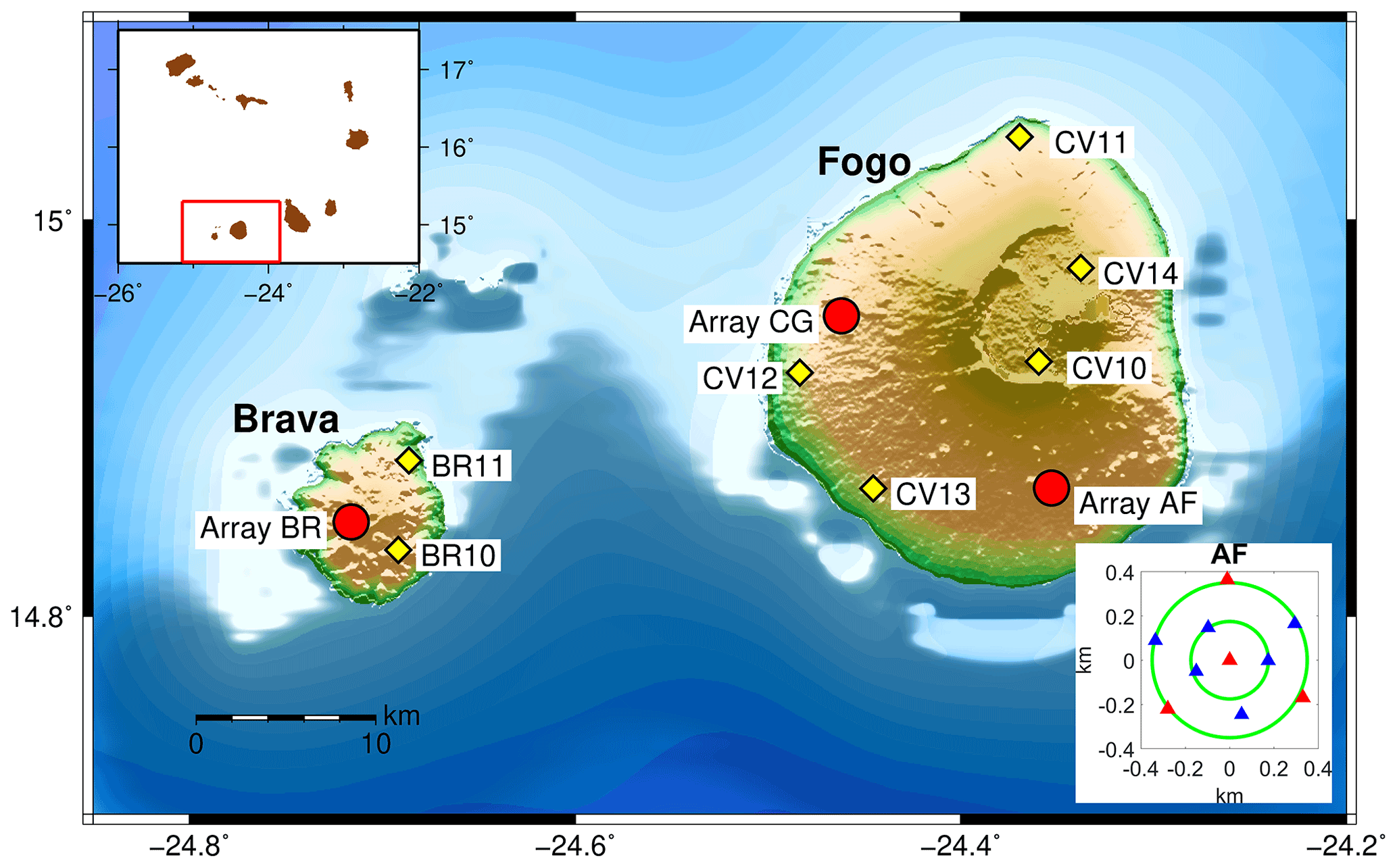
Figure 1 Station configuration on Fogo and Brava from January 2017 to January 2018. Red circles: array locations; yellow diamonds: short-period single stations. Left inset: Cape Verde, with the current section around Fogo and Brava marked in red. Right inset: setup of the array AF, red: broadband stations, blue: short-period stations. The arrays BR and CG are designed in the same way. Topography and bathymetry data are from Ryan et al. (2009).

Despite the frequent volcanic eruptions, Fogo shows a rather low rate of seismicity compared to its neighbour Brava. In Fogo, we mainly detect seismic events with a transition from high to low frequencies and without clear S phases. In a previous study by Faria and Fonseca (2014), this type of event was described as a hybrid event, as it combines features of a volcano-tectonic event in the signal onset and a long-period event with respect to the coda (see e.g. McNutt, 2000; Wassermann, 2012).

A variety of different methods exist to locate typical volcanic seismic events, depending on the characteristics of the signals. Emerging events, for example, have been analysed using probabilistic approaches to determine the maximum likelihood of the source location (e.g. Saccorotti et al., 1998; Métaxian et al., 2002; La Rocca et al., 2004). Some of these methods involve the application of a velocity model (e.g. Almendros et al., 2001a, b). In the present study, however, we focus on events which show a clear signal onset. It allows us to clearly identify the same phase at all stations and arrays. For events with a pronounced first arrival, classical beam forming can be applied and works well (Rost and Thomas, 2002; Schweitzer et al., 2012). This method can be described as a delay-and-sum procedure in the time domain. The time-domain multi-array analysis has the advantage of being independent of velocity models. The velocity structure is often very complex in volcanic environments and there is, so far, no detailed 3D-velocity model available for Fogo volcano or Brava island. The time-domain array analysis allows for the incorporation of a narrow time window while including a broad frequency band (Leva et al., 2020). As a result, the central peak of energy of the corresponding (broadband) array transfer function tends to become more narrow with side lobes suppressed (Singh and Rümpker, 2020). Traces are shifted and stacked in the time domain to increase the signal-to-noise ratio (SNR) and to retrieve information about the incoming wavefront (i.e. the back azimuth and the magnitude of the horizontal slowness, which corresponds to the inverse of the apparent velocity; Rost and Thomas, 2002). Including multiple arrays allows the localization of the event in the area of the intersected beams. In our study, we operated three arrays: two on Fogo and one on Brava, as well as seven short-period single stations from January 2017 to January 2018. We focus on volcano-tectonic earthquakes originating in the study area around Brava and Fogo and on certain volcano-seismic events on Fogo, which we, in accordance with Faria and Fonseca (2014), interpret as hybrid events. However, due to ray bending, it is possible to observe systematic deviations in back-azimuth and slowness values. To investigate these deviations at the three arrays of our study, we compare multi-array localizations with locations derived from standard (network-based) localization techniques (see e.g. Krüger and Weber, 1992). These standard techniques are based on the picking of P and S phases. For this comparison, earthquakes occurring within the network are chosen, i.e. earthquakes beneath or close to Brava or Fogo.

2 Network

From 18 January 2017 to 12 January 2018 we operated a total of 37 seismic stations on Fogo and Brava (see Fig. 1). Our network comprised three arrays each consisting of 10 stations. Two arrays were deployed on Fogo close to the villages of Achada Furna (AF) and Curral Grande (CG), and the third one was deployed on Brava (BR). Another seven stations were operated as single short-period stations to complement the network – two on Brava and five on Fogo. All seismometers used are three-component instruments.

The design of the arrays is based on the array transfer function (in terms of frequency and the slowness components). The frequencies are chosen between 5 and 10 Hz, corresponding to mean dominant frequencies of the local events. These events include volcano-tectonic earthquakes as well as other types of volcano-seismic signals such as hybrid events and harmonic tremors, the latter characterized by a frequency range between 1 and 5 Hz. Each array is circular and consists of a central station with two concentric rings with diameters of 700 and 350 m. Four of the 10 stations at each array are equipped with broadband stations and the other six stations with 4.5 Hz short-period sensors (see lower right inset map in Fig. 1). As we expect events with mean frequencies between 5 and 10 Hz, the array is optimized for mean frequencies of 7.5 Hz. The array transfer function for 7.5 Hz is shown in the Supplement (Fig. S1c). It shows a single sharp maximum of energy and only minor secondary peaks. The circular shape of the array leads to a circular, symmetric peak in energy, which allows the detection of incoming wavefronts from any direction. For comparison, the transfer functions for 5 and 15 Hz are shown in Fig. S1 as well. These conventional array responses are calculated for single frequencies. However, when performing a time-domain array analysis, a broader frequency band is implicitly incorporated. The stacking of (integration over) the array response of a wider frequency band leads to a much narrower peak. Additionally, side lobes are strongly suppressed.

3 Method and data analysis

Criteria for applicability of the classical localization of local earthquakes are clear phases of the signal and a network distributed around the origin of the signal. If these criteria are not met, array techniques can help to locate the seismic event. By beam forming, the back azimuth and the magnitude of horizontal slowness are determined. For this purpose, the coherent part of the signal is shifted in time and summed up (Rost and Thomas, 2002). This method is based on the assumption that the wavefront approaching the array approximates a plane wave, which is a valid assumption if the distance between the array and source is considerably larger than about 10 times the wavelength of the signal (Schweitzer et al., 2012).

Performing an array analysis for local events using only one array necessitates an epicentral distance estimation. In a previous study, we determined the epicentral distance based on the S–P travel-time difference. We also assumed a simplified two-layer velocity model and a fixed event depth (for details see Leva et al., 2020). However, this approach may cause significant uncertainties in the localization due to the choice of the velocity model. In the present study, to overcome this limitation, we perform a multi-array analysis. A beam, pointing towards the epicentre, is determined at each array. Transferring these beams onto a map allows determining an area of overlap. This area provides the epicentral location of an event. A main advantage of this method is its independence of a velocity model. Details of this method are described in the following sections.

3.1 Beam forming

The array analysis is performed in the time domain. The time-domain analysis is equivalent to the incorporation of a wide frequency band, while the stacking window is kept narrow around the relevant phase, e.g. the first arrival of the incoming signal (Singh and Rümpker, 2020; Leva et al., 2020). Events are detected by a trigger algorithm from the traces and chosen by the analyst for the array analysis. Traces are first band-pass-filtered within the dominant frequencies of the signal (Fig. 2). The cut-off frequencies are chosen in view of the waveform spectrogram. Following, an analysis window is chosen by the analyst around the first onset of the signal. For the local events we analyse in this study this is typically in the range of 1 to 2 s. This is shown in Fig. 3a for an example earthquake at array AF. Later, traces will be shifted within this window in reference to the trace of the central array station. A stacking window (in red in Fig. 3a) with the length of one or two periods of the signal around the signal onset marks the phase for which the beam forming is performed. This stacking window is chosen to be as narrow as possible around the first onset of the signal. Several tests showed that a length of one to two periods leads to the best results of the stacked traces and the resulting energy. However, the length is chosen individually for each array and each event. All windows are chosen in reference to the central array station. The trace of the central station is kept fixed during the time shift of the remaining traces. This time shift is performed by a grid search with slowness values from −0.3 to 0.3 s km⁻¹ and a grid size of 124×124. For each grid node traces are shifted accordingly and summed up. The resulting energy is defined by

$$E\left(t\right)=\underset{t_{\mathrm{1}}}{\overset{t_{\mathrm{2}}}{\int }}{\left[{\displaystyle \frac{\mathrm{1}}{M}}\sum _{i=\mathrm{1}}^M{x}_i\left(t+{\mathit{r}}_i\cdot \mathit{s}\right)\right]}^{\mathrm{2}}\mathrm{d}t$$

following Harjes and Henger (1973), where the waveform at station i is given by x_i and the number of stations by M. The vector r_i contains the coordinates of the array stations in reference to the central station, and the slowness vector is given by its horizontal components $\mathit{s}=\left(s_x,s_y\right)$. The resulting contour plot of the energy is shown in Fig. 3b. The slowness components s_x and s_y corresponding to the maximum energy are further used to determine slowness and back azimuth of the event. Slowness, apparent velocity and back azimuth are estimated using the expressions $\mathit{s}=\sqrt{s_x^{\mathrm{2}}+s_y^{\mathrm{2}}}$, $v_{\mathrm{app}}=\mathrm{1}/s$ and BAZ = $\left(\mathrm{180}{}^{\circ }/\mathit{\pi }\right)\arctan (s_x/s_y)$, respectively. The traces, which are shifted according to the determined slowness of the event, and the corresponding sum trace are displayed in Fig. 3c. The analogue procedure for array BR is shown in Fig. S2.1a–c and for array CG in Fig. S2.2a–c.

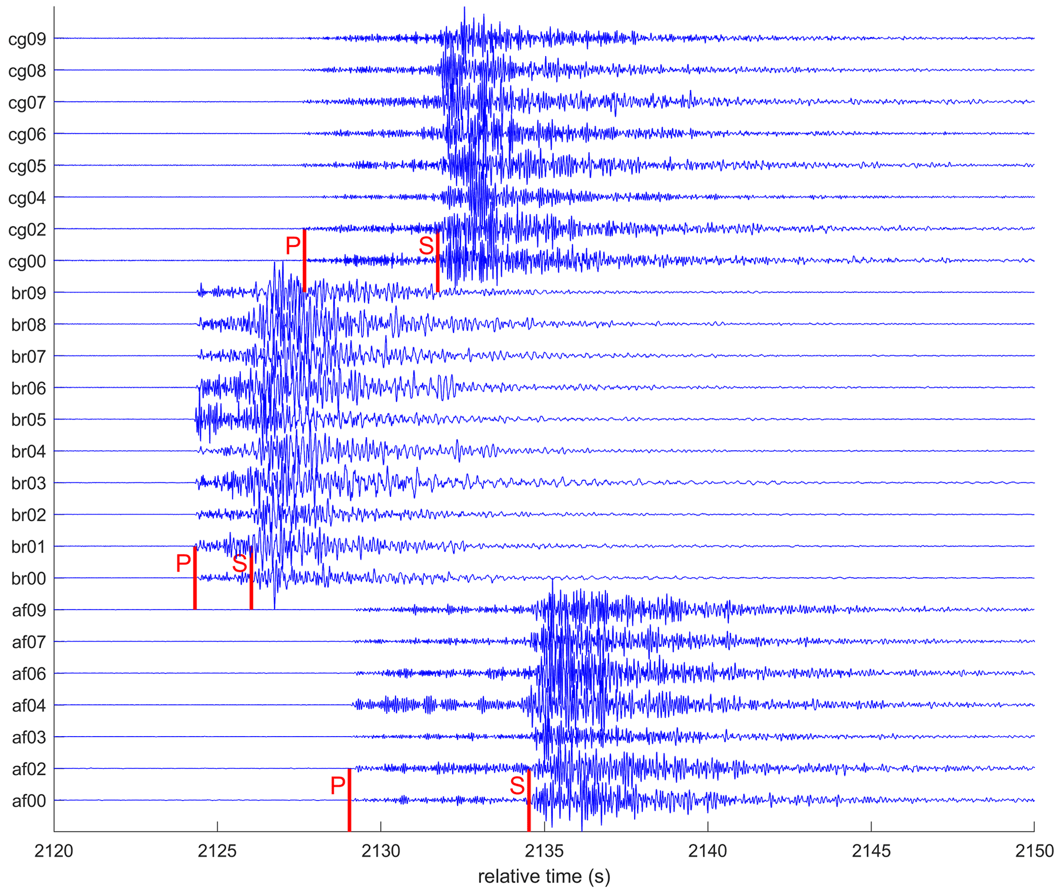
Figure 2 Z components of the seismogram of an earthquake on 22 July 2017 (23:35 UTC) before the array analysis is performed. Traces are filtered individually according to the spectrogram of each array. Filters applied here are 2–20 Hz at array AF, 2–24 Hz at array BR and 2–21 Hz at array CG. Red lines mark the P and S phases at the central array stations AF00, BR00 and CG00, respectively.

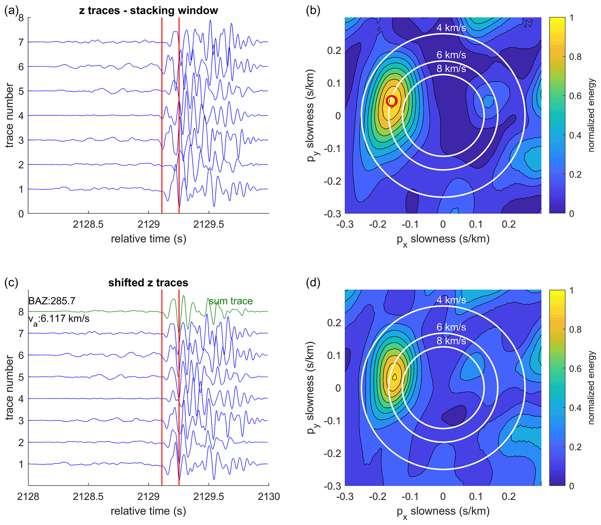
Figure 3 Time-domain array analysis of an earthquake on 22 July 2017 (23:35 UTC) at the array AF. (a) Analysis window of 2 s length with the stacking window marked in red. Traces are displayed before shifting and stacking and are filtered between 2 and 20 Hz. (b) Resulting time-domain energy stack. Red circle: maximum beam energy. (c) Time-shifted traces. The upper green trace represents the sum trace. (d) To retrieve the standard deviation of the back azimuth, the stacking window is varied 100 times by values between −0.2 and 0.2 s. The standard deviation is estimated from the 100 resulting back-azimuth values. Shown here is the stack of the 100 energy plots.

The horizontal slowness (or ray parameter) is related to the angle of incidence by $\sin \left(i\right)=s\cdot v_c$, with the velocity v_c of the upper layer beneath the array. Thus, the lower the slowness, the steeper the wavefront arrives at the array. For nearly vertical angles of incidence, the slowness s becomes close to zero and the apparent velocity approaches infinity.

3.2 Multi-array analysis

After determining the energy grid of each array, the beams are intersected in the next step to obtain the earthquake epicentre from the multi-array analysis. For the error determination, the standard deviation of the maximum energy is determined. This is estimated as a function of the chosen stacking window by randomly varying the start and end times of the stacking window 100 times by values between −0.2 and 0.2 s. The values of ±0.2 s for the variation of the start and end times of the stacking window were chosen after performing tests with values between ±0.1, ±0.2 and ±0.5 s. For the variation of ±0.1 s the standard deviation becomes very small. There is nearly no deviation from the original result, which means the resulting error is very likely underestimated and not reliable. Regarding the fact that some stacking windows are as small as 0.06 s the variation of ±0.5 s proves to be too large and often leads to stacking windows far away from the signal phase of interest. Back-azimuth and slowness values thus exhibit deviations that are far too large. Examples of the stack of the 100 energy estimations are shown in Fig. 3d for array AF, Fig. S2.1d for array BR and Fig. S2.2d for array CG. In some cases (like in Fig. S2.1d for array BR and in Fig. S2.2d for array CG) the main beam broadens, pointing to a higher sensitivity of the event at the specific array to the choice of the stacking window. If the stack of the 100 energy estimations is comparable to the original energy stack, the choice of the stacking window has nearly no impact on the determined beam.

The standard deviation of the slowness value is used as the error of the slowness at each array. In the next step the beam is determined. First, the standard deviation of the back azimuth is estimated as described above and converted into an error X in percent ($X\left[\mathit{\%}\right]=\left(\mathrm{std}\left[{}^{\circ }\right]/\mathrm{360}{}^{\circ }\right)\cdot \mathrm{100}$ %). This error is then transferred to the contour plot of energy, where the energy values within this error range are determined. This yields minimum and maximum back-azimuth values which frame the maximum peak in energy. The beam width is defined by these values, which implies that it accounts for possible uncertainties and may be asymmetric with respect to the maximum energy value. Additionally, in this way small side lobes are included in the multi-array analysis if their energy values are larger than the error (in percent) determined before. This can be seen in Fig. 4, where a small beam at array CG points to the south-southwest. The two values within which the beam is plotted are referred to as the outer range of the beam from here on. Due to possible errors and deviations of the main beam, we do not expect all three main beams to intersect in the same point; “main beam” refers to the beam with the maximum energy. The back-azimuth range defined above is used to plot the related beam. A large standard deviation leads to a broad beam (see Fig. 4, where array AF shows a standard deviation in back azimuth of ±72.8^∘). To ensure that a localization remains possible even for beams with relatively large standard deviations, a depiction of the beam energy with higher resolution would be desirable. To achieve this, we further intersect the broad beam in steps of 1 % of the error estimated from the standard deviation. Thus, we assign values from 1 (broadest beam) to 100 to each of the steps. This is further shown in Fig. S3.

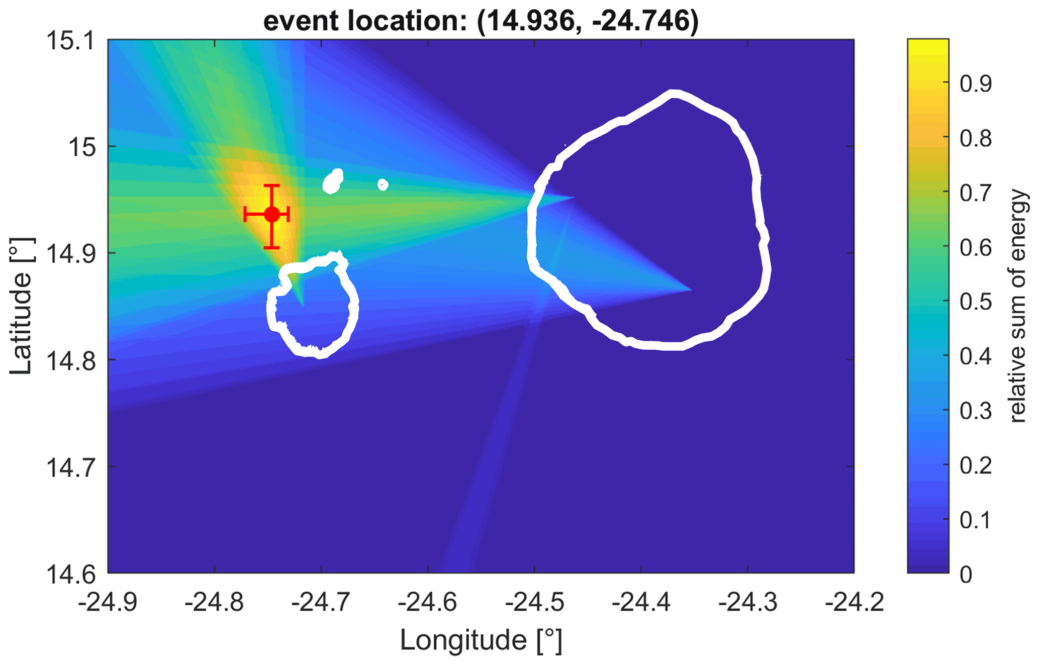
Figure 4 Intersection of the beams projected on a map section, including the coordinates of the arrays and the location of the determined epicentre. The intersected beams correspond to the example earthquake on 22 July 2017 (23:35 UTC). The small beam pointing south-southwest from array CG results from a side lobe with energy values in the range of the error corresponding to the standard deviation of the back azimuth. Red circle: event location with error bars. Topography and bathymetry data are from Ryan et al. (2009).

Now these beams are transferred to a map spanning the geographical coordinates of the research area, with the array location as the origin of the corresponding beam. The maximum value, which can theoretically be reached when intersecting the three beams, is used to normalize their values. After intersecting the beams, the area with the highest probability of the event location is determined. The last step is to choose a narrower section of the map that includes the arrays and the most likely epicentre determined in the previous step (Fig. 4).

We choose a confidence interval of 90 % of the maximum value of the intersected area as the error for the multi-array analysis.

3.3 Error considerations

Different factors have an influence on the uncertainty of the result of the multi-array analysis. They can be divided into two categories: uncertainties related to the parameters of the array analysis and due to effects of the ray paths. Parameters in connection with the analysis are the frequency range of the data and the length of the stacking window. Effects along the ray path from the source to the array, such as heterogeneities, can result in a systematic deviation of back azimuth and horizontal slowness at the array.

To test for the influence of the chosen stacking window (start and end time) and the frequencies, multiple repetitions of the analysis at one array are computed with a random variation of these parameters. Results concerning the variation of the stacking window are accounted for as described in Sect. 3.2. The same analysis has been performed for varying cut-off frequencies. For earthquakes the lower frequency is randomly varied between 2 and 8 Hz and the upper frequency between 15 and 30 Hz. For hybrid events the variation was between 1 and 4 Hz and between 10 and 20 Hz for the lower and upper frequencies, respectively. The analysis is done 100 times, and the resulting standard deviation is again used to display the energy beam in the multi-array analysis. The results for varying cut-off frequencies show a minor influence on the back azimuth, as demonstrated in Fig. S4. We conclude that, for a given stacking window, the variation of the frequency band can be neglected in the error determination. The selection of the stacking window has a larger contribution to possible errors and is thus included in the analysis, the results of which are displayed in Fig. 4. However, the choice of the stacking windows is performed individually for each array and event. One advantage of the time-domain array analysis is the possibility to focus on the very first phase of the signal. Therefore, it is preferable to select the stacking window to be as narrow as possible, as long as it encompasses the first arrival. The analyst chooses the value of the window length according to the outcome of the stacked traces and the energy plot. If the traces are not aligned properly, the sum trace displays no clear signal onset or the energy plot shows large uncertainties, as expressed, for example, by large or several side lobes. If the result is not reproducible after several trials, it is discarded from further analysis.

Velocity heterogeneities beneath the arrays or along the ray paths can possibly lead to a systematic bias in slowness and back-azimuth determination (Rost and Thomas, 2002). This deviation of horizontal slowness and back azimuth at the arrays can be determined by comparing back-azimuth and slowness values with those derived from a different localization technique (e.g. Krüger and Weber, 1992; Schweitzer et al., 2012). With respect to local events, we decided to locate earthquakes with a classical analysis (using SEISAN – Havskov and Ottemoller, 1999 – based on the HYPOCENTER code of Lienert et al., 1986) by including all single stations of our network and one station of each array. For this standard localization technique, we apply the velocity model from Vales et al. (2014). To ensure the reliability of the classical localization, only earthquakes within or very close to the network were used. This comprises only earthquakes beneath Brava or Fogo and those located between the islands. Additionally, we only used results for which the root mean square (rms) values and errors of the classical analysis are small (rms <0.25 s, errors <5 km in longitude, latitude and depth). In total, 13 events fulfilled all criteria and could be used for the comparison. Figure S5 contains a map showing the locations of the classically located earthquakes including error bars. The corresponding reference back azimuth and magnitude of horizontal slowness of these events (determined using the velocity model of Vales et al., 2014) are compared to the respective values of the array analysis. The resulting vectors, pointing with a blue line from the back azimuth and slowness value of the array analysis (red points) towards the respective values from the classical analysis, are displayed in Fig. 5. In the range of 240–270^∘, array AF systematically yields back azimuths pointing too far to the south by about 7^∘, and array CG shows back-azimuth values too far to the north with a mean deviation of about 9^∘. The values at the array on Brava show a variety of deviations due to the many directions of incoming waves. It appears that back-azimuth values in the range of 270–360^∘ point too far to the north. However, for the comparison with the classical localization, there are only four events within this range, prohibiting a reliable statement on systematic deviations.

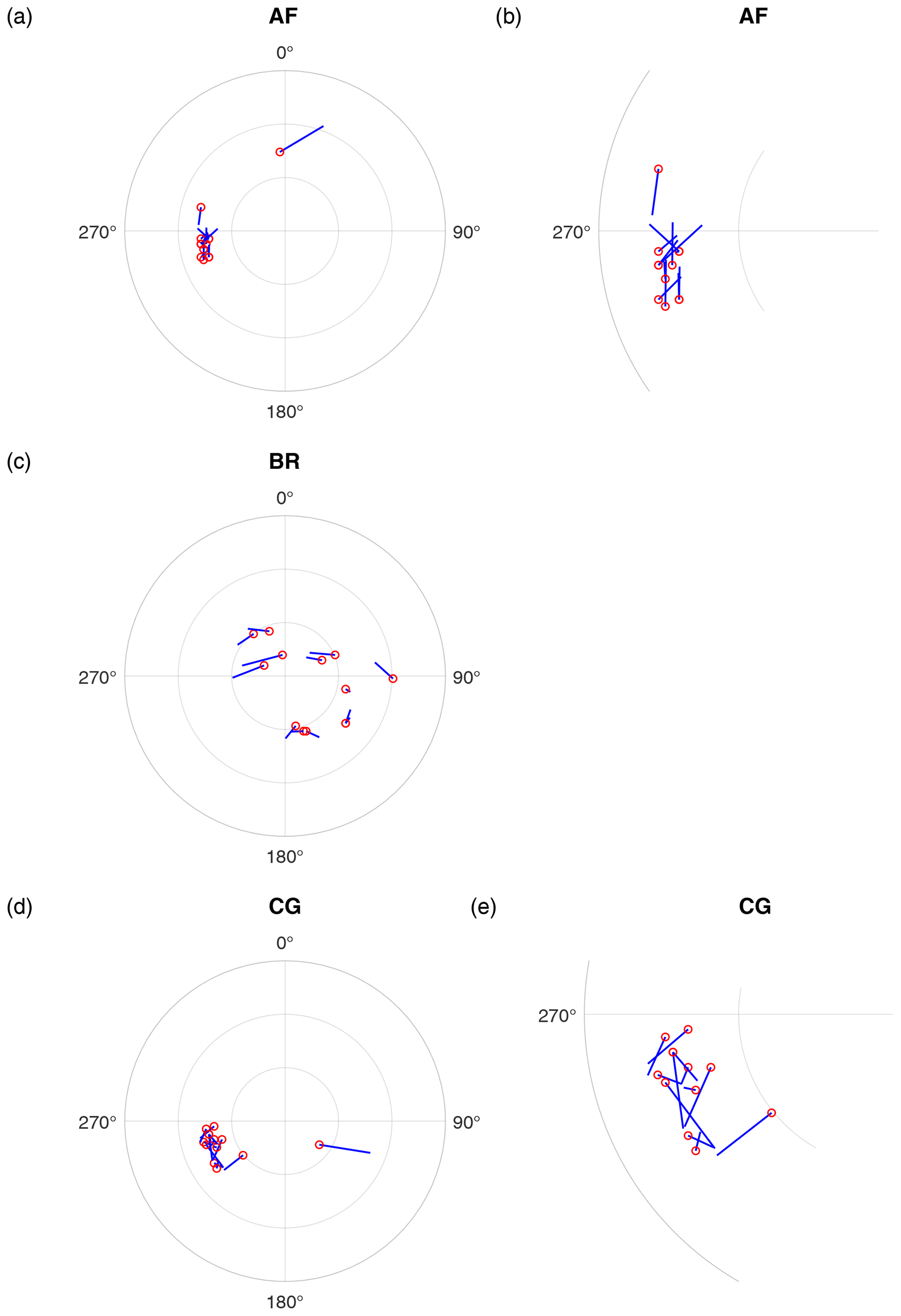
Figure 5 Deviations of back azimuth (BAZ) and horizontal slowness. Red points: back-azimuth and horizontal slowness values of the array analysis. Blue lines point towards the corresponding reference values of the standard localization. (a) Deviations of BAZ and horizontal slownesses determined at array AF. Different radii correspond to slowness values of 0.1, 0.2 and 0.25 s km⁻¹, respectively. (b) Deviations of BAZ in the range of 235 to 305^∘ and horizontal slownesses at array AF. The radii correspond to slowness values of 0.1 and 0.2 s km⁻¹, respectively. (c) Same as in (a) for array BR. (d) Same as in (a) for array CG. (e) Deviations of BAZ in the range of 210 to 280^∘ and horizontal slownesses at array CG. The radii correspond to slowness values of 0.1 and 0.2 s km⁻¹, respectively.

The station elevation differences of the array stations can have an impact on the result of the array analysis. Therefore, we carefully tested possible influences under the assumption of the different station elevations according to Schweitzer et al. (2012). It turned out that the station elevation differences are small enough to be neglected.

For a successful localization with multiple arrays certain requirements need to be fulfilled. For example, the stacking windows at each array should contain the same phase of the signal (Almendros et al., 2002). To ensure this, we perform the multi-array analysis on the first onset of the signal. Additionally, the occurrence of strong side lobes in the energy stack must be avoided as the occurrence of secondary peaks results in two or even more beams at one array. This may lead to event mislocations. Furthermore, the occurrence of strong side lobes generally indicates higher uncertainties in results. Regarding the intersection of the beams additional considerations must be taken into account. If beams trend almost parallel, the epicentre will be located far away with large uncertainty in distance (see Fig. 6a, b). Furthermore, if two beams point from one array to another, the whole area between the arrays will be a potential source region, leading to large errors in the localization (see Fig. 6c, d). In these two cases the third array is of particular importance, as it will strongly narrow down the area of the likely source. If the third array does not provide any additional information in such cases the localization of the corresponding event must be discarded due to the high level of uncertainty. Also, considering that the back azimuth and horizontal slowness show small but systematic deviations, it is not unlikely to find a result with the three beams not overlapping in the same area. To be able to assess the reliability of the location obtained during the analysis, information about the epicentral distance is added to the map of the intersecting beams. This can be used especially for the analysis of earthquakes: here, S–P travel-time differences are determined for each array. From these travel-time differences the epicentral distance of the event to each array is estimated. For this we apply a two-layer velocity model with a mean crustal and mean mantle velocity derived from Vales et al. (2014) and a fixed event depth of 5 km (see Leva et al., 2020). The fixed event depth has been defined after estimating a mean event depth from previous studies of the region around Brava (Faria and Fonseca, 2014). The resulting epicentral distances are indicated by circles, which are plotted on the map with the intersecting beams (see Fig. 7). However, this information about the epicentral distance is not included in the localization, as we want to retrieve the source epicentre without applying a velocity model. It only serves as a reference for the analyst to evaluate whether or not the estimated source location is reasonable. Due to the lack of S phases this estimate is not used during the analysis of hybrid events. However, here the array locations with respect to the event locations are very favourable, as the beams intersect almost perpendicularly. This prevents the occurrence of parallel trending beams and beams pointing towards each other.

Figure 6 Examples of problematic localizations due to unfavourable source–receiver configurations. (a, b) Intersection of the beams (a) without the beam of array BR and (b) with the beam of array BR included. In the case of parallel trending beams (a) the localization of the event is distorted and the beam of the third array is needed (b). (c, d) Intersection of the beams (c) without the beam of array AF and (d) with the beam of array AF included. In the case of beams pointing from one array to another, (c) the region of elevated energy spans a large area between the two arrays. In this case the beam of the third array is needed for a proper localization (d).

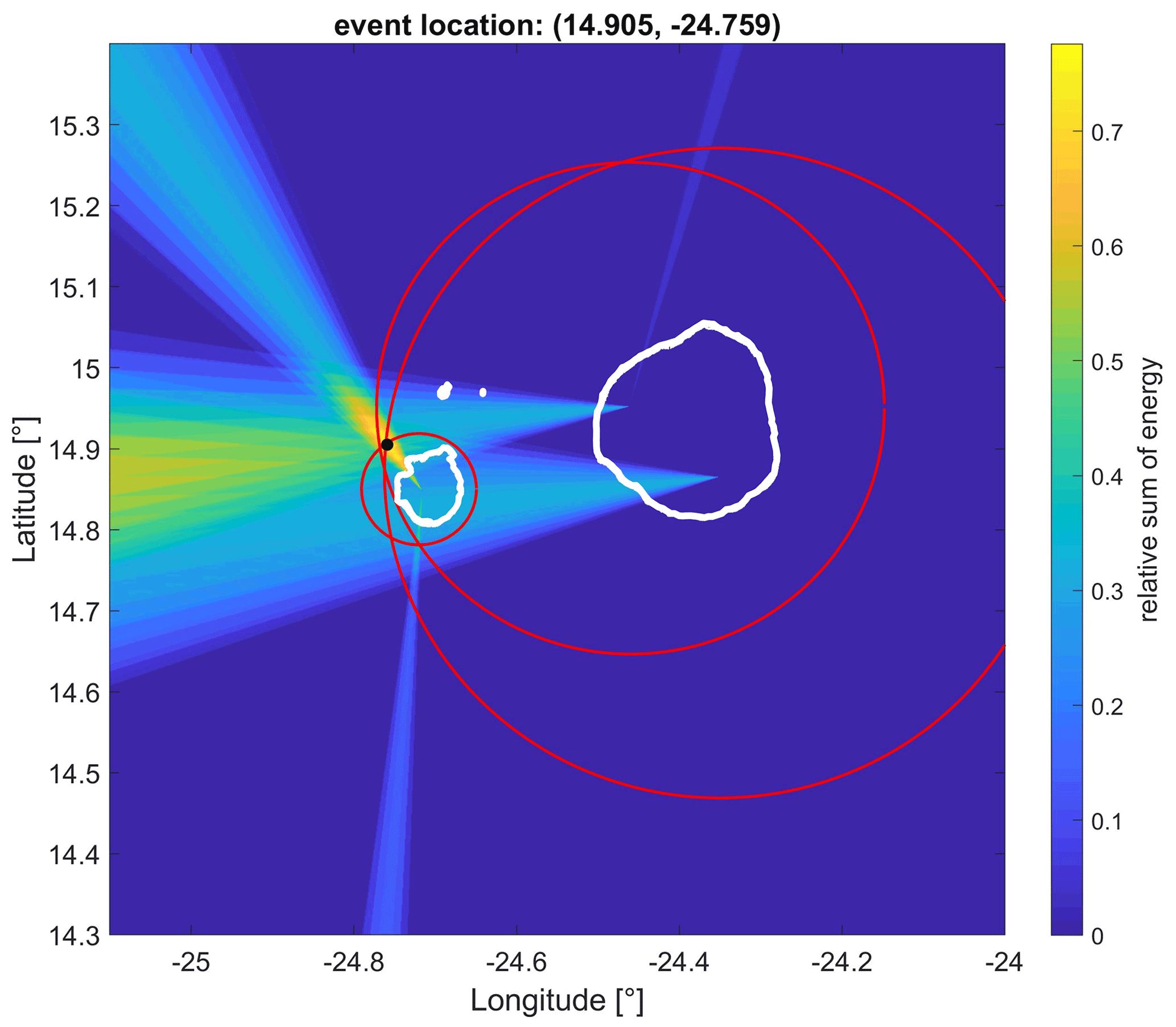
Figure 7 Verification of the event localization using additional travel-time information. Black circle: location of the event derived from the intersecting beams; red circles: epicentral distances of the event estimated from S–P travel-time differences observed at the three arrays. The circles give an estimate of the expected distance of the event to the array, providing a tool to better judge the reliability of the event location. Note that this representation only serves as support for the analyst. The final event location is only based on the multi-array analysis.

4 Results

The majority of the recorded events are local volcano-tectonic earthquakes mainly occurring in the area of Brava. However, we also observe a different type of event recorded by the stations on Fogo. These events are characterized by a smooth transition from higher (15–40 Hz) to lower (1–10 Hz) frequencies and a lack of S phases. As these are characteristics of hybrid events (e.g. McNutt, 2000; Wassermann, 2012), we follow previous studies on the seismicity of Fogo (Faria and Fonseca, 2014) and use the same terminology. Figure 8 shows traces and spectrograms of the two types of events. In the following we will focus on events which were initially detected by a trigger algorithm and selected for further analysis by visual inspection.

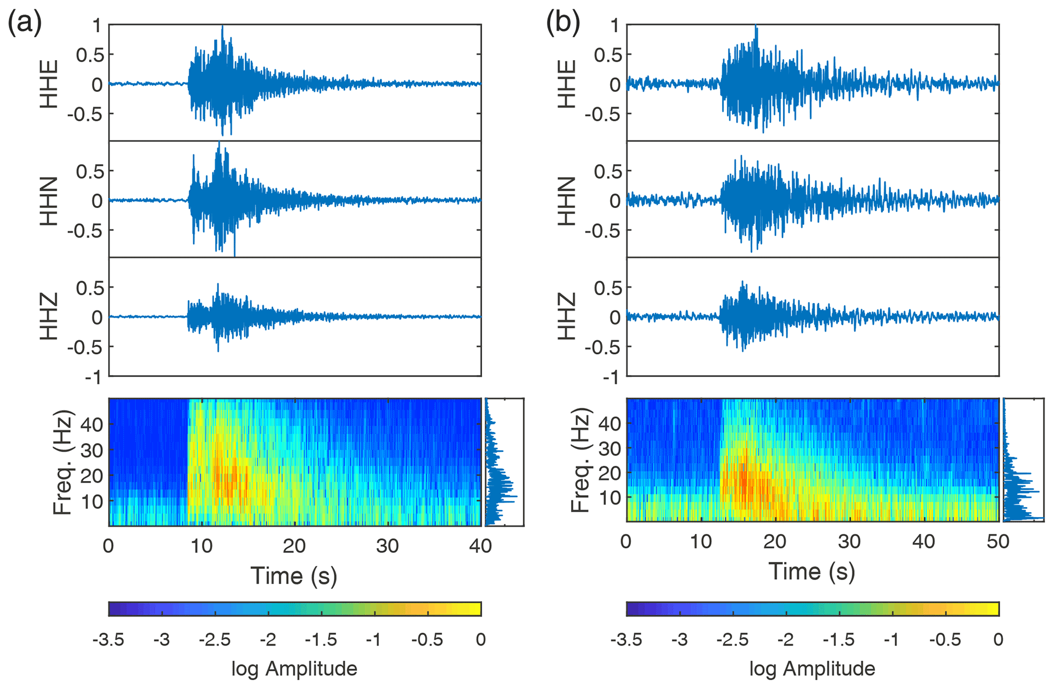
Figure 8 Comparison of a volcano-tectonic earthquake and a hybrid event. (a) Top: traces of an earthquake beneath Fogo on 18 November 2017 (04:19 UTC; event location: 15.022–24.349) recorded at the broadband station AF02 of array AF on Fogo. Bottom: spectrogram of the vertical component and overall frequency content (right). (b) Traces of a hybrid event recorded on 17 August 2017 (02:54 UTC; event location: 14.969–24.400) at the same station. Traces are filtered between 1 and 50 Hz to remove ocean-generated noise. Compared to the earthquake, the hybrid event shows no clear S phase and more energy in the 1–10 Hz band (of the coda).

4.1 Volcano-tectonic earthquakes

The volcano-tectonic earthquakes on average occur eight times a day (see Fig. 9a). The rate of seismicity frequently increases, leading to phases with elevated seismic activity. 2709 earthquakes were recorded from 18 January 2017 to 12 January 2018, 112 of which could be located using multi-array techniques. The earthquakes mainly occurred around Brava (Fig. 10). The reasons for the discrepancy in the number of detected and located earthquakes are manifold. Many smaller earthquakes are recorded with our stations only on Brava, thus precluding the multi-array analysis, as for this at least two arrays must detect the event. As described in Sect. 3.3, there may be cases in which the result of the array analysis must be discarded and cannot be used for further analysis. Thus, the multi-array analysis can only be performed for events with stable results for the back-azimuth determination. If the energy grid shows e.g. strong side lobes or the choice of slightly different stacking windows for the same event leads to strongly different results, the result of this array for this particular event is discarded. Additionally, at least two arrays must show reliable and stable results, which further reduces the number of located events. The recordings of the stations on Fogo show a rather high-frequency content with the main frequencies between 10 and 30 Hz (Fig. S6a). On Brava the dominant frequencies of the same event are lower and range between 2 and 20 Hz. The corresponding spectrum is shown in the Supplement (Fig. S6b).

Figure 9 (a) Number of earthquakes per day. Green line: accumulated number of earthquakes. The recordings range from 18 January 2017 to 12 January 2018. (b) Number of hybrid events per day. Green line: accumulated number of hybrid events during the same time period.

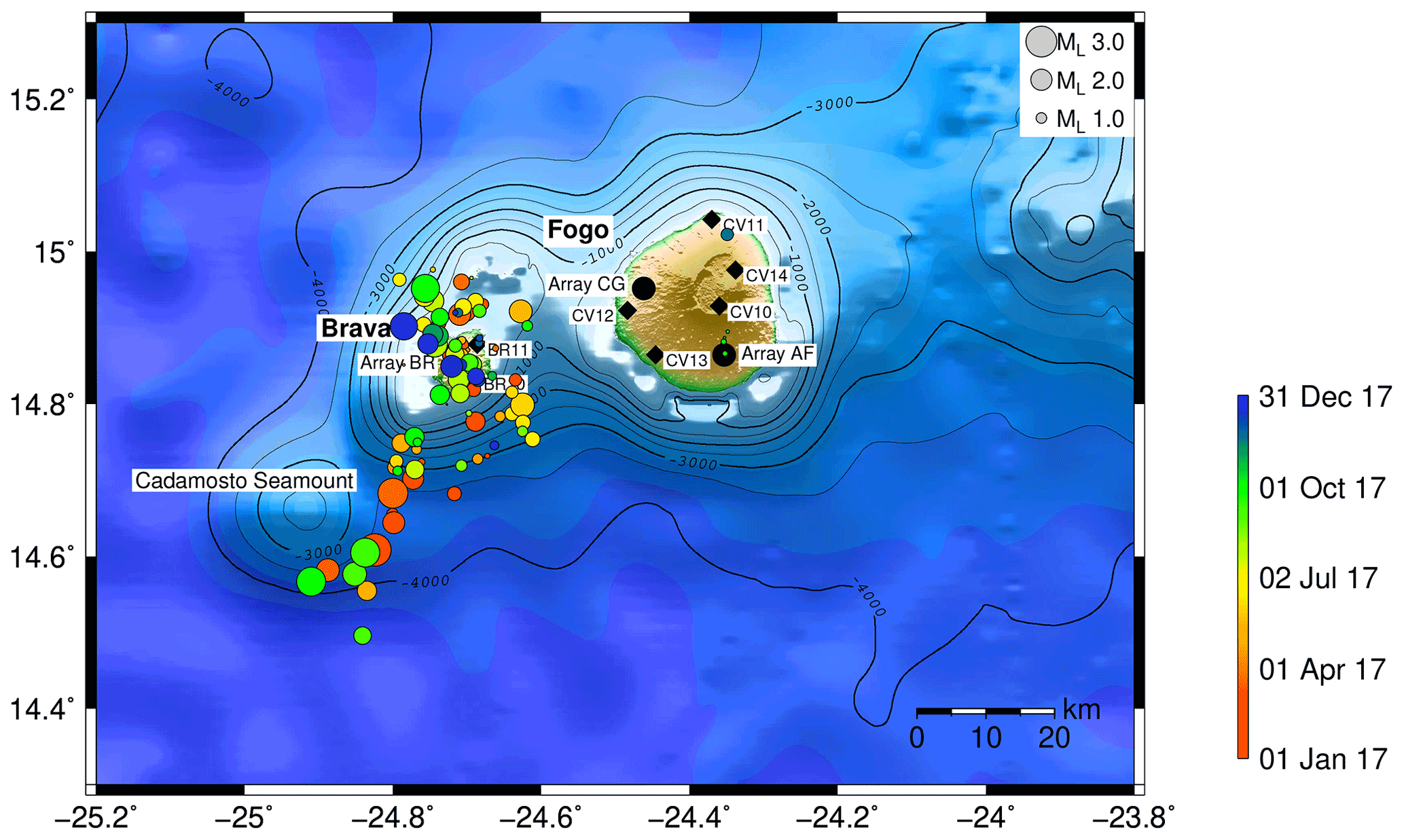
Figure 10 Earthquake locations from 18 January 2017 to 12 January 2018. Black circles: array locations; black diamonds: short-period single stations. Topography and bathymetry data are from Ryan et al. (2009).

The mean apparent velocities at the arrays on Fogo are in the range of 7.1 km s⁻¹ for events originating close to Brava. For such a distance between the event and array, the ray first propagates downwards from the source. In a medium with lateral homogeneous velocities, the apparent velocity of this ray measured at the array is equivalent to the velocity at the ray turning point. Apparent velocities <8 km s⁻¹ thus point to a ray turning point within the crust (velocity model taken from Vales et al., 2014), indicating crustal depths of the earthquakes. Note that the array on Brava shows higher apparent velocities for the same earthquakes with a mean of 10.8 km s⁻¹. However, array BR is located close to the sources, which results in a steeper angle of incidence (and smaller slowness) compared to the arrays located on Fogo.

The Supplement contains a map with error bars of the analysed earthquakes (Fig. S7).

4.2 Hybrid events

As described above, the hybrid events observed on Fogo (see Fig. 9b) are characterized by high frequencies (15–40 Hz) at the beginning of the signal, followed by low frequencies (1–10 Hz) and a lack of clear S phases. The signals mainly last about 20 to 30 s, although some last up to 1 min, and usually reach station CV10 first, where they also show the largest amplitudes. Figure 8b shows an example event recorded at a broadband station of the array AF. Vertical traces of such an event are displayed in the Supplement (Fig. S8). The spectrograms of all components are shown in Fig. S9 and reveal the low-frequency coda, with more energy occurring in the 1–10 Hz band than before the event onset. As the hybrid events were only recorded by the stations on Fogo, they were located using the arrays AF and CG. We observe 125 hybrid events, 12 of which could be located. Figure 11a shows the resulting epicentres in or close to the collapse scar of Fogo, Chã das Caldeiras. The events exhibit rather high apparent velocities: on average 7.8 km s⁻¹ at array AF and 8.4 km s⁻¹ at array CG. The mean errors of these velocities are 2.9 and 2.8 km s⁻¹ at array AF and CG, respectively. These high apparent velocities are not biased by the choice of the slowness range during the array analysis. We also tested a slowness range between −1 and 1 s km⁻¹, which does not change the outcome (see Fig. S10.1 and S10.2). To determine the source location of the hybrid events, we superimpose the beams of all localizations of the hybrid events. This is shown in Fig. 11b, where the area with the highest likelihood for hybrid event occurrence is marked by a white line (corresponding to 80 % of the maximum of the relative sum of energies). We find this area in the northwestern part of Chã das Caldeiras.

Figure 11 (a) Locations of hybrid events detected between 18 January 2017 and 12 January 2018 and located with the arrays on Fogo. Black circles: array locations; black diamonds: short-period single stations. (b) Superimposed beams of all the hybrid localizations. The white line corresponds to 80 % of the maximum of the relative sum of energy and indicates a region of high likelihood for the occurrence of hybrid events. Topography and bathymetry data are from Ryan et al. (2009).

5 Discussion

Most earthquakes occur around and beneath Brava, and the seismic activity shows several periods with increased seismicity (Fig. 9a). This is a common observation for the seismicity around Brava (Faria and Fonseca, 2014; Vales et al., 2014; Leva et al., 2020). The earthquakes originate in the crust as derived from the apparent velocities measured at the arrays. Performing the time-domain array analysis allows for the determination of the epicentre of small local earthquakes (M_L<0.5), although the P-wave arrival is not clearly visible at all stations. However, their combination during the beam forming results in a clear P-phase onset of the sum trace. The application of the time-domain array analysis is favourable in such a case, as a wide frequency band can be chosen to optimize the SNR. It is worth noting that the frequency content of the earthquake recordings on Brava generally exhibit lower dominant frequencies (Fig. S6b) than the recordings of the same events on Fogo (Fig. S6a). This is surprising, as higher frequencies are typically more attenuated. On the other hand, observations of high-frequency tremors around Fogo have been described by Heleno et al. (2006). These authors report on the conservation of high frequencies in a tremor signal even at larger distances (about 15 km) from the source. In September we observe some earthquakes beneath Fogo (see Fig. 10) which occur within the shallow crust according to the apparent velocities measured at the arrays and the S–P travel-time differences. These events are located close to the area where deep subcrustal earthquakes were observed in August 2016 (see Fig. S11; Leva et al., 2019). Nevertheless, due to their large difference in depth and the long amount of time between these two occurrences, we cannot establish a link between them (as due to the transport of magma from depth into the crust).

Apart from the earthquakes in September, Fogo mainly shows volcanic seismic signals which are best described as hybrid events (in total 125 in 2017). Their origin is located in the northwestern part of the collapse scar of Fogo and on top of the Bodeira wall, which surrounds large parts of the collapse scar Chã das Caldeiras. It has been discussed in previous studies (e.g. McNutt, 2000; Wassermann, 2012) that these events are caused by a combination of source mechanisms relevant for volcano-tectonic earthquakes and long-period events. One such hypothesis is a volcano-tectonic earthquake which triggers the oscillation of a fluid-filled cavity (McNutt, 2000). At Fogo, hybrid events have been detected before (Faria and Fonseca, 2014). They were attributed to hydrothermal processes at shallow depths (several hundred metres) due to the interaction of rainwater and hot rock. This hypothesis is based on the seasonal variation of the number of hybrid events and a water table found at 370 m depth in the Chã das Caldeiras. We observe a variation in the number of events over the year of observation and compared it with the amount of precipitation per month in 2017. The corresponding figure is shown in the Supplement (Fig. S12). We find an increase in hybrid events from February to March and from September to November. The precipitation shows a small peak in March, which might correspond to the peak of hybrid events. However, the strongest peak of precipitation occurs in August. This does not directly correlate with the maximum peak in the number of hybrid events, which occurs in November. From this, we conclude that a causal relationship between precipitation rates and the occurrence of hybrid events cannot be established.

High apparent velocities of the hybrid events indicate steep angles of incidence, possibly pointing to a deep-seated source. With the multi-array analysis applied in this study, it is not possible to estimate the depth of the events, as we do not include a velocity model. However, for an estimate of the source depth of the hybrid events, it is possible to derive the ray path under consideration of a simple velocity model and the angle of incidence. The velocity model is adapted from Vales et al. (2014) with velocity increasing at steps of 0.1 km. For this approach the modification of the velocity model was necessary to allow for an incremental ray bending according to Snell's law. The ray path is traced back from the angle of incidence at the array until the epicentral distance is reached. This simple model yields event depths of 5 to 14 km. The uncertainties are relatively large. For some events the depth estimates at the two arrays can lead to different results, which points to inconsistencies likely related to the insufficient (1D) velocity model. Additionally, we considered other velocity models, which might be better suited regarding the expected complex velocity structure. Adapting a velocity model for Etna (Almendros et al., 2000) yields event depths between 10 and 20 km. The use of the velocity model for the caldera of Tenerife (Lodge et al., 2012) yields results between 3.5 and 15 km. This shows the significant impact of the velocity model on the estimation of the angle of incidence at the array and the computed ray path. The event depths estimated from the slowness values observed at the arrays and the different velocity models would be significantly deeper than the depths reported in previous studies. There can be several reasons for such an observation. It is possible that the source of the events shifted to greater depths after the eruption of Fogo in 2014. This might also explain why there is no direct correlation between the precipitation data for 2017 and the number of hybrid events. Another possibility is that the wave field is affected by path effects caused by the complex structure of the volcanic edifice (Kedar et al., 1996). Kedar et al. (1996) suggest that a single pulse can trigger seismic waves, which then interact with heterogeneities in the elastic, loosely consolidated surrounding layers of the volcanic edifice, leading to complex harmonic seismic signals at the receiver. Such an effect is hard to discriminate from an oscillating resonator. Finally, Harrington and Brodsky (2007) provide the explanation that hybrid events are not necessarily caused by fluid motion, but by brittle failure. Low rupture velocities and strong path effects result in the long low-frequency coda. Similar effects of low rupture velocities in unconsolidated volcanic material have also been suggested to cause the signature of long-period events rather than fluid-driven source mechanisms (Bean et al., 2014). On Fogo, brittle failure at shallow depths could be caused by gravity loadings in the collapse scar after the latest eruption. In view of these previous studies and our observations, i.e. the clear signal onset, the lack of S phases and the smooth transition from high to low frequencies without the appearance of definite dominant frequencies, we suggest that scattering effects along the ray path may explain the distinct appearance of the hybrid events on Fogo.

A complex ray path might also affect the slowness measured at the arrays. Almendros et al. (2001a) evaluate the influence of a complex 3D velocity structure of Kilauea, Hawaii, on the apparent velocity recorded at a seismic array. The results point to a reduction of the slowness values in comparison to a homogenous velocity model. It is likely that the complex velocity structure of Fogo has an impact on the ray path and thus leads to slowness variations. This bias could possibly result in smaller slowness values and thus explain the high apparent velocities we measure. However, the assumed uncertainties of the apparent velocities are rather large and should cover this bias. In addition to these considerations, we observe strong differences in the amplitudes at the stations. The amplitudes of hybrid events at station CV10 in the collapse scar are nearly twice as large as the amplitudes of the other stations on Fogo not located this close to the source. The second station, CV14, in the collapse scar was only operational during the last 3 months of the study. However, for the few events detected in this period, the amplitudes at CV14 are in the range of those at CV10, but the signal arrives slightly later than at station CV10. If the events actually occurred at depths of 5 to 14 km, we would not expect such a large difference in the amplitude ratios. For earthquakes occurring on Fogo or Brava, the amplitudes at station CV10 are in the range of the amplitudes at the other stations. A bias due to site effects at this station is thus unlikely. We thus conclude that despite the high apparent velocities, the hybrid events should actually originate from shallower depths, as already suggested by previous authors (Faria and Fonseca, 2014). Nevertheless, a hydrothermal origin may not be necessary to explain their occurrence, and their real cause remains unclear. The use of a high-resolution 3D velocity model or a dedicated dense network of stations placed near the observed epicentres could contribute to a better understanding of these events, as it would allow for a more precise depth estimate.

Being independent of any velocity model and able to locate the epicentres of events without a clear onset of phases or occurring offshore outside the network are strong advantages of the utilization of multiple seismic arrays. However, there are certain limitations of the multi-array analysis. The back azimuth and slowness determined with the arrays on Fogo and Brava show a systematic deviation, which has been estimated by a comparison with classically located events. The number of reference events (in total 13) is too small for a correction of back-azimuth and slowness values during the analysis. However, some relevant conclusions can still be drawn for the utilization of the multi-array technique. At the arrays AF and CG on Fogo wavefronts arrive from a range of back azimuths of 240 to 270^∘ (see Fig. S13.1). Within this range the back-azimuth values show a mean deviation to the south of 7^∘ at array AF and a mean deviation to the north of 9^∘ at array CG. For the array BR on Brava observed back-azimuth values cover a wide range (see Fig. S13.1) and slowness values can be small for events close to the array. Figure 5 shows larger deviations of back azimuth and slowness for events with horizontal slowness values below 0.1 s km⁻¹. The question arises of whether the results of array BR should generally be discarded when they show horizontal slowness values below 0.1 s km⁻¹. However, the beams related to the arrays on Fogo can easily trend almost parallel, leading to an overestimated epicentre distance (based on comparison with the S–P travel-time difference, see Fig. 7). Therefore, the beam of the array on Brava is essential, as it usually locates the event closer to the expected location. This is shown in Fig. 6a and b. Generally, the errors in the event locations, which result from the uncertainties of the back-azimuth determination at array BR, are by far smaller than the errors when using only the arrays on Fogo. The distance estimated from the S–P travel-time difference serves as verification of the epicentral distance determined by the multi-array analysis (see Fig. 7). This is especially helpful when only two arrays are available for a localization. Thus, a multi-array analysis using only two arrays is still possible but might lead to a certain number of earthquakes that cannot be located due to the deviation of back-azimuth values. For the hybrid events on Fogo, the determination of the deviation vectors is not possible due to the lack of reference localizations. The distribution of back-azimuth values of the hybrid events is displayed in the Supplement (Fig. S13.2). The back-azimuth values clearly indicate a location close to or in the collapse scar of Fogo. Nevertheless, a possible deviation should not lead to large errors in the localization because of the location of the arrays with respect to the source region.

6 Conclusion

From January 2017 to January 2018, we operated three arrays on Fogo and Brava to apply a time-domain multi-array analysis for seismic events occurring in this region. This application allows epicentral event localization without assuming a velocity model. This is a significant advantage in volcanic environments where the velocity structure is difficult to constrain. Additionally, we are able to determine the epicentre of offshore earthquakes outside the network and hybrid events without clear S phases. Although the application of the time-domain multi-array analysis has many benefits, it is necessary to evaluate possible errors of the localization, which may result from systematic deviations of back-azimuth and slowness values determined at the arrays. These deviations can be caused by heterogeneities along the ray path. To determine the deviations of back-azimuth and slowness values, we compare them to those derived from a classical earthquake analysis. It turns out that the number of reference events is too small for a reliable correction. We therefore allow for relatively large location uncertainties to cover the possible deviations.

A large number of volcano-tectonic earthquakes are located beneath and around Brava. As reported previously (Faria and Fonseca, 2014; Vales et al., 2014; Leva et al., 2020), we observe several periods of elevated seismic activity and a frequent shift of locations around the island. Additionally, a few earthquakes occur beneath Fogo in the shallow part of the crust. Some of them occur in the shallow crust in approximately the same epicentral area as deep subcrustal earthquakes of 2016 (Leva et al., 2019). However, a conclusion concerning a possible link between these two occurrences could not be made due to the rareness of such earthquakes. However, the majority of seismic events beneath Fogo are hybrid events. As shown by a joint analysis of the events, their epicentres are close to the northwestern part of the Chã das Caldeiras and beneath the Bodeira wall. These events show larger apparent velocities than the volcano-tectonic earthquakes recorded with the arrays on Fogo. Most likely, these high values result from the influence of the topography and the complex velocity structure of the volcanic edifice, leading to a possible bias in the slowness determination. Additionally, the station CV10 located in the Chã das Caldeiras shows significantly larger amplitudes than the remaining stations on Fogo. We believe that the origin of the hybrid events is not as deep as the high apparent velocities would suggest. However, the origin remains unclear due to the lack of information about the depth. The application of a precise 3D velocity model or a dedicated local network could shed further light on the depth and thus on the possible source mechanism of these events.

In addition to the volcano-tectonic earthquakes and the hybrid events, we detected isolated instances of volcanic tremors, which we have not yet analysed in detail. This will be the subject of forthcoming studies.