Upper-lithospheric structure of northeastern Venezuela from joint inversion of surface-wave dispersion and receiver functions

We use 1.5 years of continuous recordings from an amphibious seismic network deployment in the region of northeastern South America and the southeastern Caribbean to study the crustal and uppermost mantle structure through a joint inversion of surface-wave dispersion curves determined from ambient seismic noise and receiver functions. The availability of both ocean bottom seismometers (OBSs) and land stations makes this experiment ideal to determine the best processing methods to extract reliable empirical Green's functions (EGFs) and construct a 3D shear velocity model. Results show EGFs with high signal-to-noise ratio for land–land, land–OBS and OBS–OBS paths from a variety of stacking methods. Using the EGF estimates, we measure phase and group velocity dispersion curves for Rayleigh and Love waves. We complement these observations with receiver functions, which allow us to perform an H-k analysis to obtain Moho depth estimates across the study area. The measured dispersion curves and receiver functions are used in a Bayesian joint inversion to retrieve a series of 1D shear-wave velocity models, which are then interpolated to build a 3D model of the region. Our results display clear contrasts in the oceanic region across the border of the San Sebastian–El Pilar strike-slip fault system as well as a high-velocity region that corresponds well with the continental craton of southeastern Venezuela. We resolve known geological features in our new model, including the Espino Graben and the Guiana Shield provinces, and provide new information about their crustal structures. Furthermore, we image the difference in the crust beneath the Maturín and Guárico sub-basins.

1 Introduction

The southeastern Caribbean and northeastern Venezuela area (i.e., 6–14^∘ N, 69–60^∘ W), located on the border between the Caribbean and South American plates, is a structurally complex area (Fig. 1) with active seismicity across multiple fault systems, the transition from oceanic to continental crust, a variety of sedimentary basins and a continental craton.

The current Caribbean Plate configuration results from a transpressive deformation (e.g., Pindell et al., 1988; Meschede and Frisch, 1998; Müller et al., 1999), with a southern border dominated by strike-slip fault systems (e.g., Russo and Speed, 1994; Sisson et al., 2005). This region is also located between two major subduction zones: the Lesser Antilles to the east and south and the Middle America trench to the west. One of the most important features of northeastern Venezuela is the eastern Venezuela Basin (Rohr, 1991). This structure, formed by oblique compression during the Oligocene to Miocene, is one of the world's most important petroliferous basins (e.g., Yoris and Ostos, 1997). The Guiana Shield, a continental craton formed during the Proterozoic–Archean, lies to the southeast of the basin (Fig. 1) and is one of the largest and oldest and a highly stable tectonic features in South America. The western part of the Guiana Shield (formed around 3–2.8 Ga, as part of the Guriense orogeny) consists of metasedimentary rocks, including granitic gneiss and granitic intrusions that have been metamorphosed to amphibolite and granulite facies (e.g., Sisson et al., 2005). The eastern section of the Guiana Shield (2–2.7 Ga age) is primarily composed of metasedimentary rocks and mafic to felsic volcanic material, locally intruded by gabbro and diabase (Arnaiz-Rodríguez and Orihuela, 2013).

In terms of geodynamics, the plate interaction between the Caribbean and South American plates is evolving at a rate of 1–2 cm yr⁻¹ westward (e.g., Pérez et al., 2001; DeMets et al., 2010; Hodgkinson et al., 2015; Jouanne et al., 2011; Reinoza et al., 2015; Pousse Beltran et al., 2016), subducting the South American lithosphere beneath the Lesser Antilles (e.g., Avé Lallemant, 1997; Jácome et al., 2003; Pindell et al., 2005). The detected seismicity in this region (as shown in Fig. 1 using data from 2005 to 2020) is sparse west of 65^∘ W; however, an important cluster stretches between the Peninsula of Paria and the island of Trinidad. The earthquakes in this cluster range from shallow to intermediate depths (∼40 to 150 km), and their magnitudes vary from M_w 3 to 5, with a few relatively large events (M_w≈6.5). The Paria cluster contains a gap in seismicity between 36–51 km depth that Clark et al. (2008) used to conclude that the subducting and buoyant pieces of the South American Plate occur along a near-vertical tear and support a “jelly sandwich” rheology.

In this work, we study the structurally complex NE Venezuela region through ambient noise tomography (ANT), which is a well-known tool developed in the last few decades (e.g., Shapiro et al., 2005) that is capable of imaging the crust and upper mantle. The most important step in ANT is the extraction of high-quality surface-wave empirical Green's functions (EGFs) from cross-correlations of seismic ambient noise (e.g., Bensen et al., 2007; Schimmel et al., 2011; Ventosa et al., 2019). Theoretical studies have proven that the EGFs between two points can be estimated from the cross-correlation of the diffuse wave field (e.g., ambient noise, scattered coda) recorded at the two locations when noise sources are well distributed (Harmon et al., 2007; Campillo et al., 2011). However, only a few studies, at either regional or local scales, use EGFs retrieved from ocean bottom seismometers (OBSs) to obtain ANT from onshore to offshore regions (Tian et al., 2013; Lee et al., 2014; Corela et al., 2017; Ryberg et al., 2017; Hable et al., 2019). The use of ANT methodologies with OBSs presents several major difficulties in comparison with continental stations. Frequently, seismic energy recorded by the OBSs is contaminated by low-frequency oceanic infragravity waves (Webb, 1998; Bell et al., 2015; Tian and Ritzwoller, 2017). Additionally, the OBS instruments can be affected by local conditions, such as interactions of ocean currents with the sea floor that can cause tilting noise (Webb and Crawford, 1999; Deen et al., 2017).

The study area has previously been imaged using passive seismic techniques such as finite-frequency P-wave tomography (Bezada et al., 2010), analysis of 20–100 s period earthquake-derived Rayleigh waves (Miller et al., 2009) and investigation of Rayleigh-wave phase velocities extracted from seismic ambient noise (Arnaiz-Rodríguez et al., 2021). Previous studies have also resolved Moho depths in this area through receiver function (RF) analysis (Niu et al., 2007) and wide angle active seismic profiling (e.g., Schmitz et al., 2008, 2021, and references therein). In this work, we combine the seismic ambient noise tomography approach with the information provided by receiver functions. Our joint inversion of these two datasets provides more strongly resolved models than finite-frequency P-wave tomography for the crust and upper mantle. Additionally, our joint inversion overcomes limitations of surface-wave tomography alone, including non-uniqueness, poorly constrained shallow structure and poor sensitivity to interfaces, such as the Moho. These advantages enable us to gain new insights into the study region.

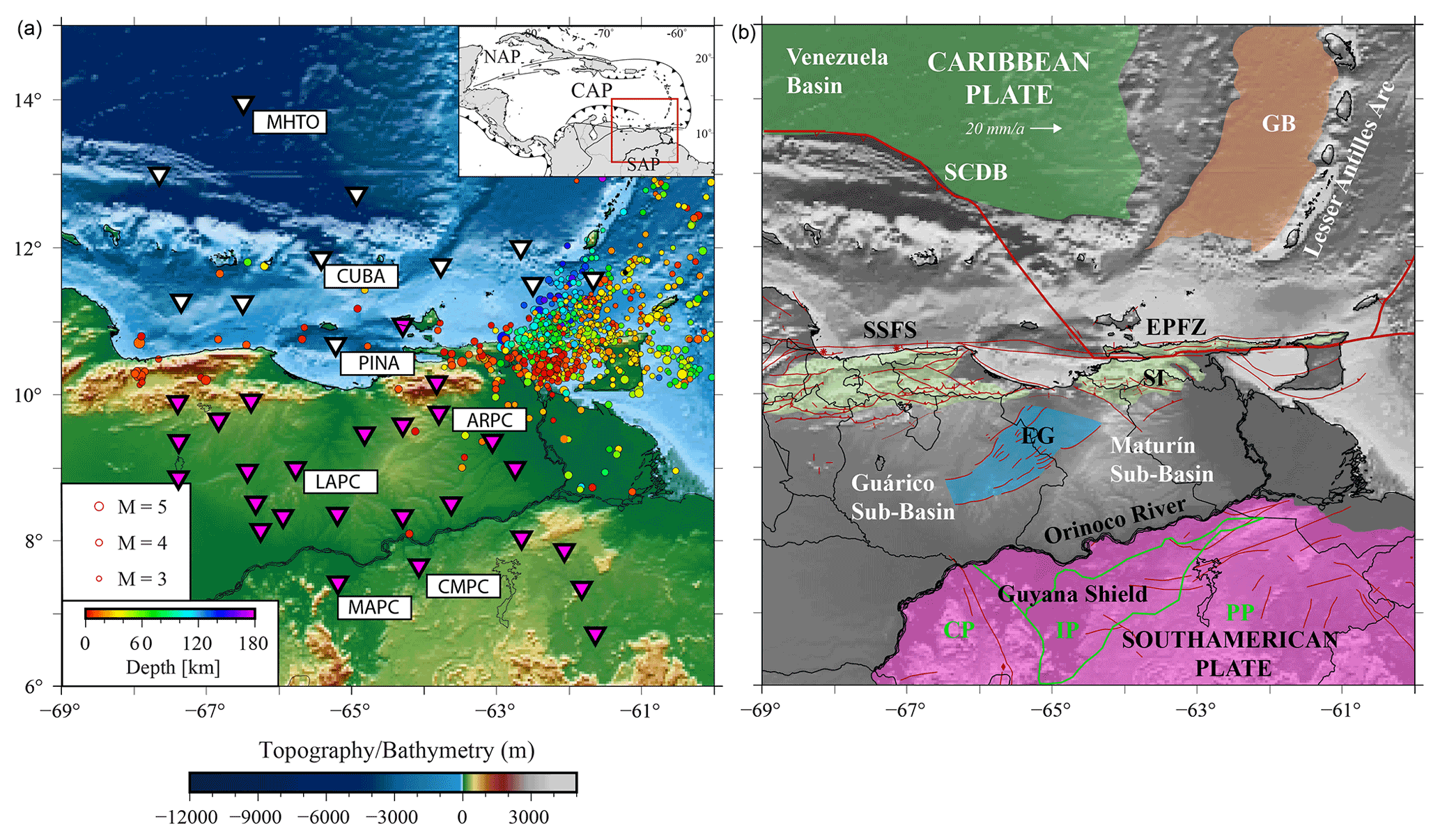
Figure 1 (a) Topographic map of the studied area overlaid with stations (triangles) from the BOLIVAR project (2004–2005). The local seismicity (circles) from 2005–2020 (M_w>3.0) is shown to illustrate the tectonic background and complexity of the study region (see main text). On the top right is a view of the general context of the Caribbean Plate and northern South America. Blue triangles represent stations inland, while white triangles represent OBS. Labeled stations are later used to illustrate methodology and results. (b) Simplified geologic map of the studied region. The Precambrian shield is shown in purple, the Jurassic Espino Graben (EG) in blue, in green the Serranía del Interior (SI), in dark green the Cretacic Venezuela Basin and in brown the Grenada Basin. In red we show active faults as presented by Audemard et al. (2006). Other abbreviations include SSFS (San Sebastian Fault System), EPFS (El Pilar Fault System), Trinidad and Tobago (TT), Peninsula of Paria (PoP), Cuchivero Province (CP), Imataca Province (IP), and Pastora Province (PP).

Specifically, we use a joint inversion of ANT and RFs using a non-linear inversion based on the Markov chain Monte Carlo (MCMC) methodology. Through cross-correlating 1.5 years of data, we extract 6 to 32 s period fundamental-mode Rayleigh and Love waves recorded at 38 broadband stations. The results are discussed with reference to previous studies (Niu et al., 2007; Schmitz et al., 2008; Miller et al., 2009; Bezada et al., 2010; Arnaiz-Rodríguez et al., 2021; Schmitz et al., 2021) and how our findings enable us to characterize known tectonic features as well as obtain new information.

2 Data and methods

Data for this experiment (Vernon et al., 2003) were collected with a sampling rate of 100 Hz at 27 land stations (STS-2/Quanterra-330) and 11 broadband OBSs (Trillium-40 s) from the Ocean Bottom Seismograph Instrument Pool (OBSIP). The minimum interstation distance is 30 km, and the aperture of the complete seismic network is approximately 1000 km. Both vertical- and horizontal-component recordings are used from the land stations, but only the vertical component is considered from the OBSs due to contamination of the horizontal components with oceanic noise (Webb, 1998).

In the following sections, we briefly describe the steps that we followed to build the EGFs from the ambient seismic noise recordings. Overall, we have closely followed the approach described by Bensen et al. (2007) but with modifications in the preprocessing stage to obtain clear, reliable results for the OBSs. Then, we discuss how we retrieved measurements of group and phase velocities for both Rayleigh and Love waves from the EGFs, which we then used to build a set of phase and group velocity maps for the studied region. Next, the computation and analysis of the receiver functions are discussed. Finally, we describe the joint inversions of the phase and group velocity maps and of the receiver functions that we performed to obtain a 3D shear-wave velocity model of the studied area.

2.1 Empirical Green's functions (EGFs)

In the first preprocessing step, daily seismograms are analyzed and removed if they are found to contain glitches or gaps in more than 5 % of the daily record to prevent artifacts in later processing steps. Next, we down-sample the seismograms to 5 Hz for computational efficiency. Then we remove the mean and deconvolve the instrument response (converting the seismograms to velocity) and rotate the horizontal components between stations to obtain the transverse component (T), except for the OBSs. This allows us to obtain estimates of the EGFs for the transverse components directly, from which we extract dispersion measurements for the Love waves. We apply absolute mean time normalization to remove unwanted earthquake contamination (Bensen et al., 2007) for each station on the vertical and transverse components independently. To form the temporal normalization function we apply a bandpass filter of 0.01–0.05 Hz and apply a running absolute mean with a window of 128 s. We divide the data from each station and component by the temporal normalization function. Next, we perform spectral whitening to expand the frequency band and balance persistent sources of noise (Ritzwoller et al., 2001; Lin et al., 2008). We divide the spectrum of each station and component by its smoothed, 0.025 Hz (20 points half-width) running-mean spectrum.

Finally, we compute cross-correlations on 4 h segments of the preprocessed seismograms (vertical–vertical, Z–Z) and (transverse–transverse, T–T) for every pair of stations. Although the linear stack is the common approach to compute the EGFs, we prefer to consider the timescale phase-weighted stack (ts-PWS) (Ventosa et al., 2017, 2019) to enhance the quality and increase signal-to-noise ratio (SNR) of the EGFs. The complex frame used in the wavelet approach of the ts-PWS is a computationally efficient method for large datasets in comparison with the conventional PWS.

Figure 2 displays both kinds of stacks (linear and ts-PWS) of the vertical components for different paths after filtering the EGFs with a bandpass filter (6–10 s). It is clear from Fig. 2 that, in general, the ts-PWS yields higher signal-to-noise ratio results than the linear stack, especially for noisy stations, such as OBSs or stations in areas with thick sediments (Cabieces et al., 2020).

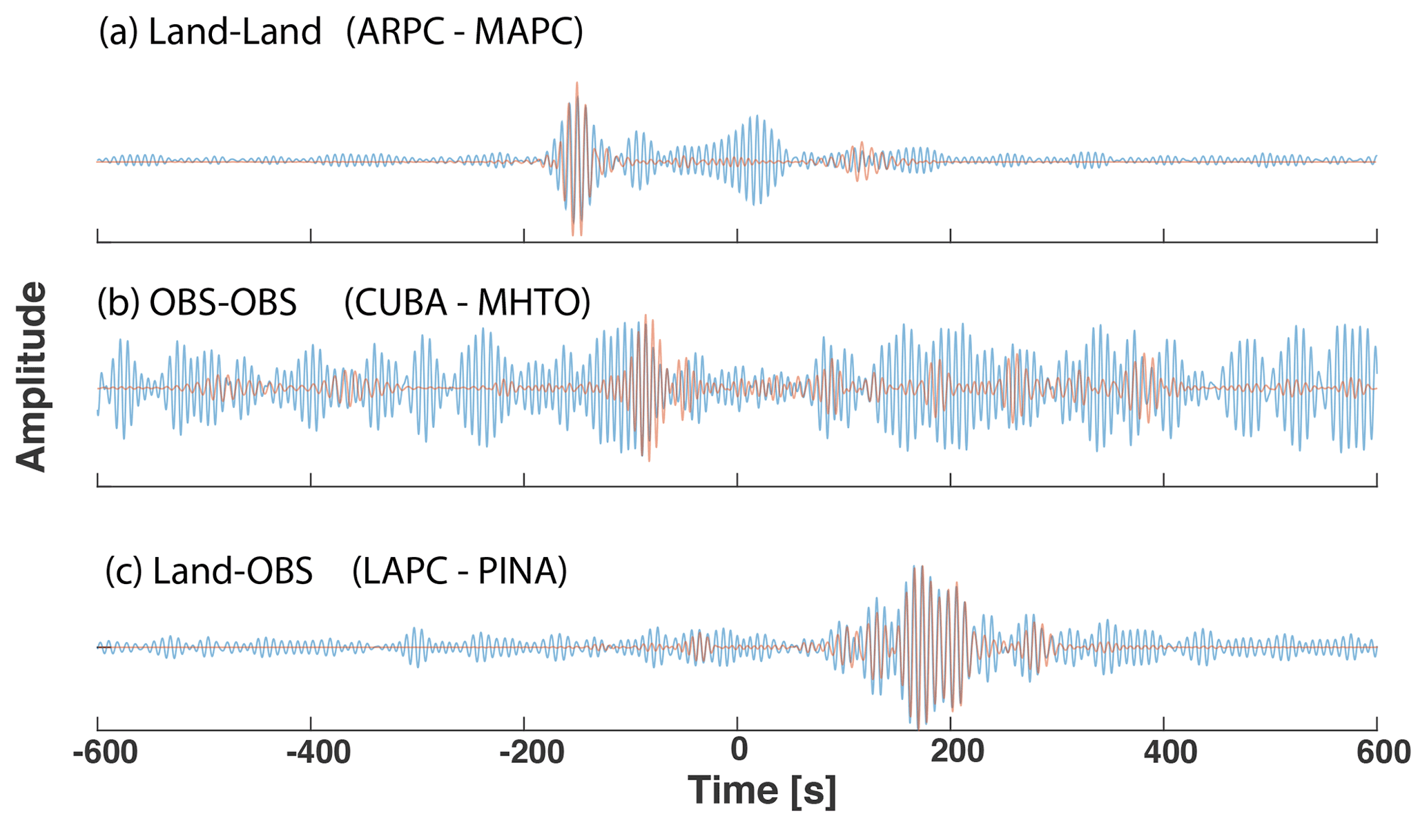
Figure 2 EGFs from three different cross-correlation pairs (EGFs) determined via linear stacking of cross-correlograms (blue) and ts-PWS stacking of the cross-correlograms (red). All EGFs are bandpass-filtered over 6–10 s. This includes EGFs from (a) land stations ARPC to MAPC, (b) OBS stations CUBA to MHTO, and (c) land–OBS stations LAPC to PINA, respectively. See Fig. 1 for station locations.

The EGF estimates contain two signals, the causal (positive lag time) and the acausal (negative lag time), which are symmetric in an ideal case. However, the spatial and temporal variation in the noise source distribution strongly affects the shape of the EGFs in the time domain and may also induce perturbations of the spectral energy content. Figure 3 displays the record section of the Z–Z and T–T correlations with the CMPC station, located in the Guiana Shield. Many of the noise cross-correlations in the study area (e.g., OBSs and land stations placed north of the Orinoco River) are non-symmetric. This is generally associated with the uneven distribution of ambient noise sources in the region (e.g., Webb, 1998; Arnaiz-Rodríguez et al., 2021). In this case, we expect the strongest pulses coming from the Caribbean Sea, where strong storms and hurricanes generally cross it in the E–W direction. We see strong differences in amplitude between the causal and the acausal portions for both components, but broadly these are more pronounced in the T–T component. To reduce the influence of seasonal variations (Tanimoto et al., 2006; Schimmel et al., 2011) and potential impact of oceanic waves dominating the noise field (Hillers et al., 2013), we average the causal and the acausal part of the EGFs (shown in Fig. 3 for the CMPC station, located in the Guiana Shield).

Figure 3 Record section of Guiana Shield station CMPC (see Fig. 1). Specifically, we show the non-symmetric, stacked EGFs between CMPC and all of the rest of the stations. (a) Vertical–vertical (Z–Z) component where EGFs from CMPC–land stations are shown as black lines and EGFs from CMPC to OBSs as red lines. (b) Same as (a), but for the transverse–transverse (T–T) component EGFs.

2.2 Dispersion measurements of phase and group velocity

We obtain fundamental-mode phase and group velocity estimates for both Rayleigh and Love waves in a period band ranging from 6 to 32 s. We manually pick these dispersion curves using the Computer Programs in Seismology (CPS; Herrmann, 2013) software. In order to use only the most reliable EGFs, we impose several criteria, including a minimum signal-to-noise ratio (SNR >40) in the period band T ∼0.5–100 s to reject unstable EGFs and a minimum interstation distance of three wavelengths (Boschi et al., 2013; Luo et al., 2015) to satisfy the far-field approximation.

Figure 4 summarizes the dispersion curves calculated from the vertical (Fig. 4a) and from the horizontal (Fig. 4b) components for land–land, ocean–ocean and land–ocean cross-correlations. This includes dispersion curves from cross-correlation of ARPC to MAPC, two land stations that cross from the Guiana Shield toward the Maturín sub-basin, labeled in Fig. 1. The ARPC–MAPC dispersion curve shows the typical behavior of a continental region, with low velocities slowly increasing in the intermediate period range (T ∼10–30 s). Figure 4 also shows the dispersion curve measured for the CUBA–MHTO pair, two OBS stations, in which the most interesting feature is the higher velocities in the same period range, highlighting the crustal thinning occurring towards the north of the study area and sensitivity of these measurements to the transition from the crust to the upper mantle. Finally, results for the LAPC–PINA station pair in Fig. 4 illustrate the results obtained from the cross-correlation of a land station and an OBS station, respectively. The LAPC–PINA station pair dispersion curve also shows a steep gradient curve due to the path through the oceanic region, but its velocity is lowest among the other dispersion curves shown in this example.

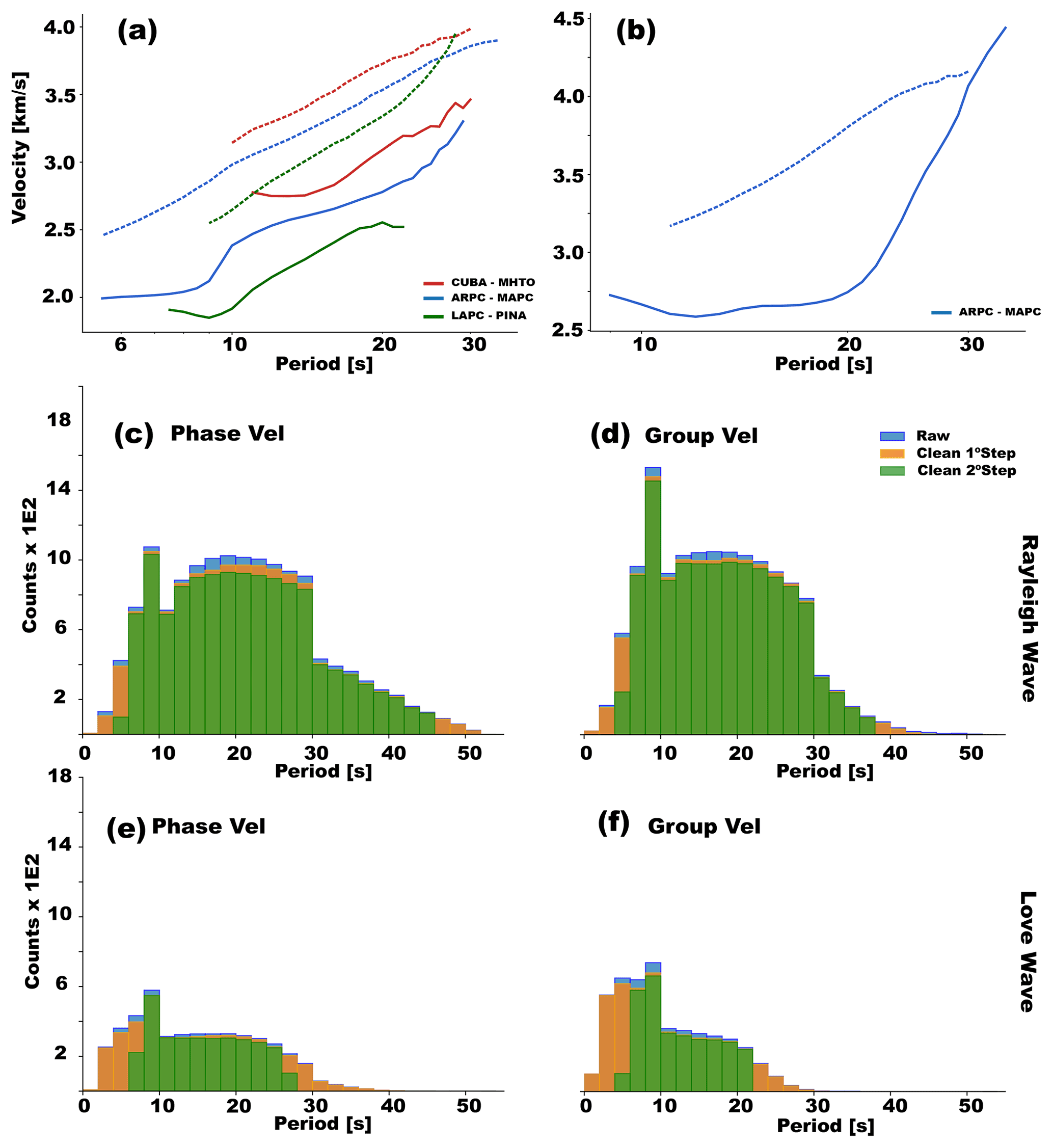
Figure 4 Dispersion curves for multiple EGFs and station pair waveforms corresponding to those shown in Fig. 2 (see Fig. 1 for station locations). (a) Rayleigh-wave dispersion curves for phase velocity (dashed lines) and group velocity (solid lines). (b) Love-wave dispersion curves for phase velocity (dashed lines) and group velocity (solid lines). Note that only land–land stations are viable for Love-wave dispersion analysis. (c, e) Phase velocity histograms of dispersion measurements for Rayleigh and Love waves, respectively. (d, f) Love velocity histograms of dispersion measures for Rayleigh and Love waves, respectively. Blue bars correspond to raw measurements, orange bars correspond to measurements obtained after cleaning by smoothing the phase/group dispersion maps (α=2000), and green bars are the final measurements obtained after excluding outliers that are outside of 3 standard deviations for a given wave period.

The measurements of phase and group velocity from all station pairs in different periods can be used to form histograms that help to visualize outliers (Figs. 4 and S1 in the Supplement). These histograms show that our measurements of group and phase velocity are most stable between periods of 6 and 32 s. The group and phase velocity values with periods outside of a maximum cut-off of 3 standard deviations were discarded to remove erroneous measurements that could negatively impact the tomographic inversion. For this same reason, those periods with fewer than 100 valid measurements are also automatically rejected.

2.3 Phase and group velocity maps

We use the fundamental-mode Rayleigh- and Love-wave group and phase velocity measurements to produce a set of isotropic group and phase velocity maps following the inversion procedure described by Barmin et al. (2001) as implemented by Olivar-Castaño et al. (2020). In this approach, we discretize surface-wave velocities across the study area (phase or group) along a regular grid (10×10 km in this study) and linearize the travel time inversion by assuming that surface waves travel along the great circle paths between respective station pairs. We minimize the misfit to the observed travel times to resolve the velocity maps. We regularize the problem through multiple constraints, including a smoothing condition (controlled by a parameter α) and a penalization for deviations from the average velocity in areas of poor data coverage (controlled by a parameter β). One of the advantages of this method is the ability to estimate data covariance and spatial-resolution maps.

The travel time inversion procedure is performed twice to remove outliers (Barmin et al., 2001). First, the phase velocity maps are over-smoothed by setting a very high value for α. Second, the observed travel times are compared with those computed using the over-smoothed maps. The measurements corresponding to residuals greater than 3 standard deviations are discarded (Moschetti et al., 2007).

We empirically derive the optimal inversion parameters to minimize model residuals and prevent sharp artifacts (Barmin et al., 2001). Additionally, the final choice of regularization parameters (α=600, σ=250, β=10) reproduces several smooth features that are consistent with known geological features of the study area, as shown in maps of Rayleigh (Fig. 5) and Love (Fig. 6) phase and group velocity results.

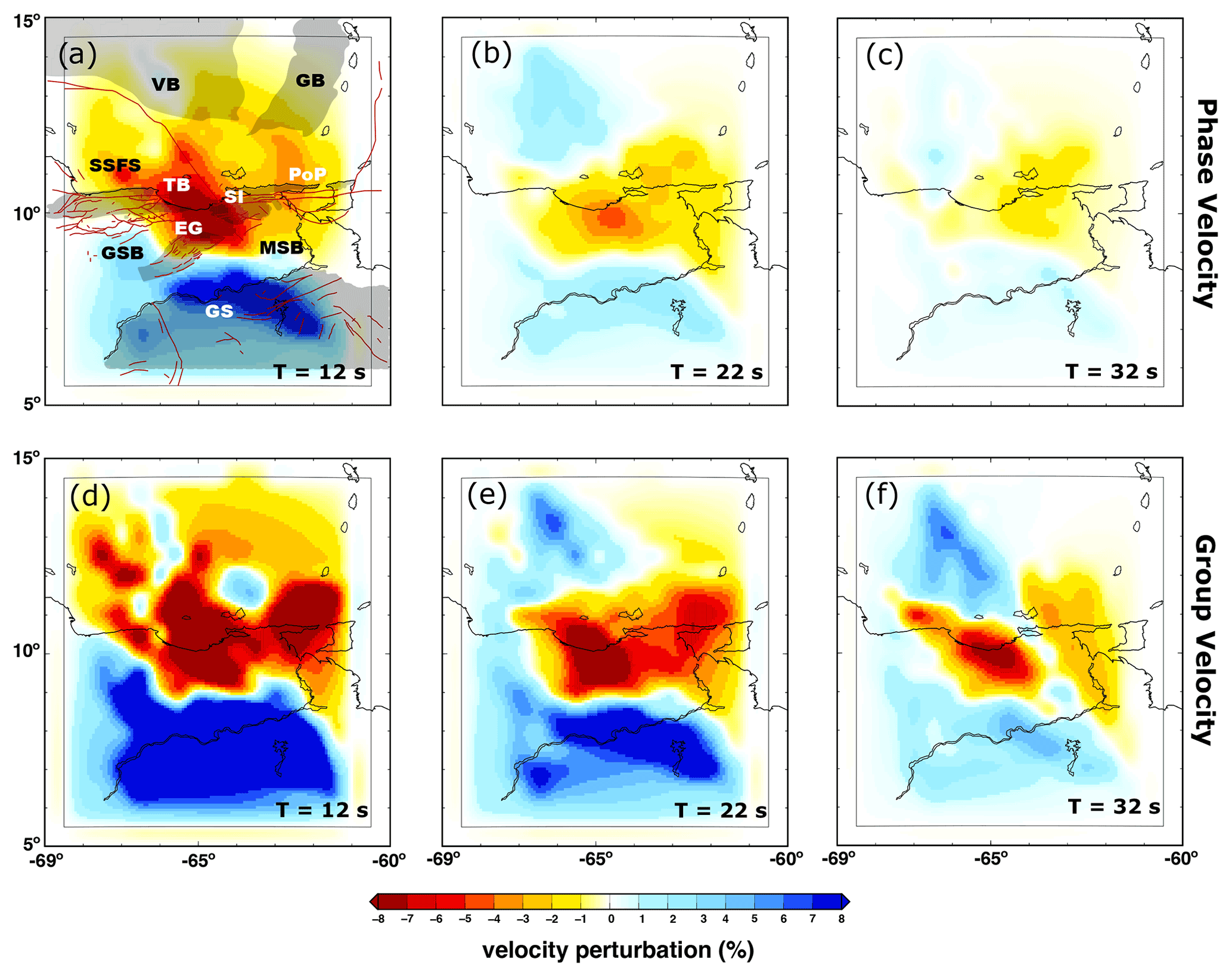
Figure 5 Rayleigh-wave phase (a–c) and group velocity (d–f) maps for wave periods of T 12, 22 and 32 s. The gray box denotes the area with reliable measurements based on ray-path coverage. In red we show active faults as presented by Audemard et al. (2006). Abbreviations are VB (Venezuela Basin), GS (Guiana Shield), MSB (Maturín sub-basin), GSB (Guarico sub-basin), SI (Serrania del Interior), EG (Espino Graben), TB (Turtle Island–Barcelona Bay), PoP (Peninsula of Paria) and SSFS (San Sebastian Fault System). VB, GB, SSFS, EG, SI, PoP and GS regions are highlighted with shaded areas.

The ray-path coverage is shown in the Supplement for both Rayleigh and Love waves. We highlight the ray-path coverage and velocity maps for the periods of 12, 22 and 32 s for the Rayleigh-wave group and phase (Figs. S2 and S3, respectively) measurements. We also include the Love-wave group and phase (Figs. S4 and S5) ray-path coverage and velocity maps for 12 and 20 s periods. We use the ray-path coverage and spatial-resolution maps (Figs. S8 and S9) as a proxy to determine where we expect reliable group and phase velocity results. In order to further evaluate the limitations of our group and phase velocity maps, we performed a checkerboard test (Figs. S6 and S7). The size of the velocity anomalies that we try to recover in the checkerboard tests is period-dependent (equal to one wavelength). The results of these tests indicate stronger constraint of velocity anomalies in the south (Guarico and Maturín basins) than in the region covered by OBSs, and overall, we see higher spatial resolution for Rayleigh waves than for Love waves.

2.4 Station orientation and Moho depth estimation

Accurate orientation of the horizontal components of the seismic stations is critical, to obtain both reliable receiver functions and Love-wave velocity estimates, especially when using OBSs. The SNR of the RFs calculated in a misoriented station is generally diminished, and the peaks associated with the Moho depth can be shifted. We have oriented the OBSs used in this work following the methodology of Doran and Laske (2017). Their method takes advantage of Rayleigh-wave ellipticity to orient the horizontal components. The goal is to find the maximum correlation between the Hilbert transform of the vertical component and the horizontal component in a time window that contains a Rayleigh wave generated by a shallow teleseism. Correct timing for the windows is determined using global dispersion maps of Rayleigh waves (Ma et al., 2014).

To perform this analysis, we use all available earthquakes with magnitudes ranging from 5.5 to 8.0, epicentral distances ranging from 5 to 165^∘ and a maximum depth of 150 km (∼100 events). Orientation results for the OBS stations and their associated uncertainties are shown in the Table S1 in the Supplement.

One of the most important constraints required to obtain geologically reasonable solutions from the inversion of dispersion curves of surface waves is a reliable Moho depth estimation, as the surface waves in the period range considered in this study only weakly constrain the deeper crustal structure.  We obtain Moho depth estimates across the study area through an H-k analysis of the receiver functions (Zhu and Kanamori, 2000) computed for both the land stations and the OBSs, using the Integrated Seismic Program (ISP) (Cabieces et al., 2022) as shown in Sect. 3.2. To estimate the receiver functions, all events with M_w>5.5 and epicentral distances ranging from 30 to 90^∘ from March 2004 to March 2005 (∼100 events) were considered. Theoretical first arrival times were computed for each event and station using the TauP library (Crotwell et al., 1999), and the continuous waveforms were cut 10 s before and 80 s after the computed first arrival times.

First, we rotate the waveforms from the ZNE to the LQT reference system. Since the back azimuth of the P-to-S-converted arrivals might deviate slightly from that of the great circle linking the event epicenter with the receiver, we investigate a suite of rotation angles following Wilde-Piórko et al. (2017). We then compute receiver functions through the water-level deconvolution technique (Langston, 1979), which suppresses instabilities in the spectral division of the L and Q components via the water-level filter. We also apply a Gaussian filter in the deconvolution process to ensure that the resulting receiver functions do not suffer from misleading high-frequency content (Langston, 1979). Depending on the SNR of the resulting receiver functions, the values of the water-level parameter and Gaussian filter width used in this study range from 0.01 to 0.0001 and 2 to 4, respectively.

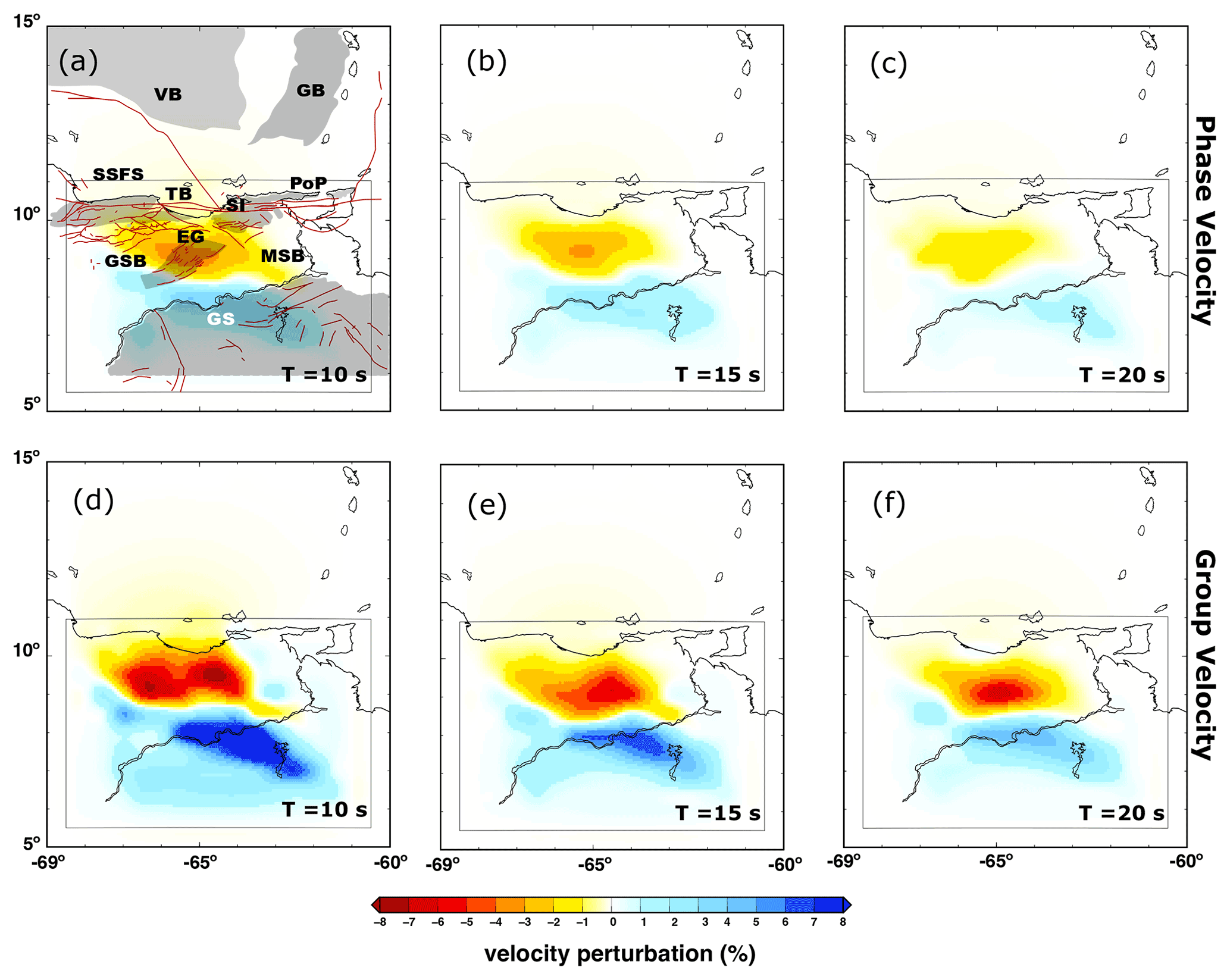
Figure 6 Similar for Fig. 5, but for Love-wave phase and group velocity maps for wave periods of 10, 15 and 20 s. In red we show active faults as presented by Audemard et al. (2006). Abbreviations are VB (Venezuela Basin), GS (Guiana Shield), MSB (Maturín sub-basin), GSB (Guarico sub-basin), SI (Serrania del Interior), EG (Espino Graben), TB (Turtle Island–Barcelona Bay), PoP (Peninsula of Paria) and SSFS (San Sebastian Fault System). VB, GB, SSFS, EG, SI, PoP and GS regions are highlighted with shaded areas.

Finally, to incorporate the receiver functions into the joint inversion with the phase and group velocity of surface waves, we determine the isotropic component of the receiver functions via harmonic decomposition (e.g., Shen et al., 2013). The isotropic component represents the velocity contrasts directly below the recording station and, in theory, reduces the effects of any lateral heterogeneities (Bianchi et al., 2010). Moreover, the harmonic decomposition technique allows us to estimate an uncertainty range for the receiver functions to be used in the joint inversion (see Sect. 3.2).

2.5 Joint inversion for shear-wave velocity

We perform a 1D inversion at each point within the grid with a resolution of $\mathrm{0.5}\times \mathrm{0.5}{}^{\circ }$ (5.5–14.5^∘ N, 68.5–60.5^∘ W) using the corresponding phase and group velocity dispersion curves extracted from the maps discussed in Sect. 2.4. Next, we jointly invert the dispersion curves and the receiver functions in the closest grid points to a station (distance $<\mathrm{0.5}{}^{\circ }$) using the Markov chain Monte Carlo (MCMC) Bayesian inversion tool BayHunter (Dreiling et al., 2020). This algorithm is inspired by the methodology of Bodin et al. (2012), in which the Bayesian formulation is applied to foster a posterior probability distribution, where each model parameter can be described with a full probability density function. Bayesian inversions have an important advantage over deterministic methods due to their exploration across a wide range of velocity models, making the choice of initial models less critical. Additionally, Bayesian inversions enable calculation of final model uncertainty from the posterior distribution and determination of data sensitivity to the model space (Shen et al., 2013; Berg et al., 2020). In addition to obtaining the velocity–depth structure, the BayHunter algorithm resolves the probability distribution of the $V_{\text{p}}/V_{\text{s}}$ ratio, the optimal number of layers of the model and the noise parameters (i.e., data noise correlation and amplitude) within a user-defined range.

In terms of inversion parametrization, we searched over a range of shear-wave velocities (V_s) from 2 to 6 km s⁻¹ (based on existing geological information); $V_{\text{p}}/V_{\text{s}}$ from 1.6 to 1.9; a maximum of 20 layers; and decreased and increased tolerance limits of V_s with respect to depth of 10 % and 75 %, respectively. To further reduce the non-uniqueness of the inverse problem and help to discard geologically implausible results, we restricted the Moho depths to a broad range (±5 km) centered in the depths estimated from the H-k stacking of the receiver functions. These constraints on the Moho depths were applied to inversions performed at geographic points closer than 0.5^∘ from the seismic stations. The uncertainties in the amplitudes of the σ surface-wave dispersion curves (SWDCs) and σ RF were set from 0 to 0.1 km s⁻¹, the correlation parameter for the SWDCs was set to 0.2, and that for RFs was set to 0.96.

While our MCMC joint inversion includes both surface-wave and receiver function data with the objective of a best-fit V_s model, we also include a prior constraint on the Moho depth. The Moho depth is obtained in the H-k analysis of the receiver functions. At each inversion point, we ran a total of 40 Markov chains with a final distribution of 100 000 iterations per chain, keeping all models within an accepting rate of 40 % to form the posterior probability distribution, with a 2:1 ratio for the burn-in and exploration phases, respectively. We tried that range of values for the set of inversion parameters, in line with accepting rates of previous studies (e.g., Bodin et al., 2012; Dreiling et al., 2020), and we found that they led to stable results and reasonable computational efficiency.

3 Results

3.1 Phase and group velocity results

The fundamental-mode phase and group velocity maps of Rayleigh (Fig. 5) and Love (Fig. 6) waves show patterns related to the main geologic structures, including the Maturín Basin (Moho depth ≈ 45 km) and Guiana Shield (Moho depth ≈35 km). Both sets of results in Figs. 5 and 6 are displayed as percent perturbation of the mean velocity for three representative wave periods, with the corresponding spatial-resolution maps in the Supplement (Figs. S8 and S9). Relatively low phase and group velocities are recovered for the Guarico and Maturín sedimentary sub-basins. These low-velocity anomalies are stronger towards the southern parts of these basins, suggesting increased sediment thickness typical of foreland basins. However, these low velocities are not observed south of the basins in the transition to the Guiana Shield (Jácome et al., 2003). The contrast between the lower relative velocities of the Maturín Basin and the higher velocities of the Guiana Shield is especially evident in the phase and group velocity maps of Love waves (Fig. 6a–f), which are more sensitive to near-surface structure than their Rayleigh-wave counterparts (Lin et al., 2008).

The velocity contrast between the oceanic crust and the sedimentary basins can also be seen in the Rayleigh-wave group and phase velocity maps, most prominent at longer periods (Fig. 5b–c, e–f). However, as the depth sensitivity of the surface waves increases with increasing periods, this contrast becomes more apparent at larger periods (e.g., Fig. 5f). We also note that the San Sebastian–El Pilar fault system appears as a sharp boundary, separating regions of different velocities in the northeast along the Peninsula of Paria and Trinidad and Tobago (see Fig. 5e, f). Overall, the spatial-resolution values for the phase and group velocity maps remain stable at ∼130–150 km in the central part of our studied area, where the data coverage is high (Figs. S8 and S9). Some elongated features can be observed on the southeastern end of the studied area (around the Orinoco Delta), which could be interpreted as smearing effects due to the sparser data coverage in this region. Therefore, in the discussion section we mainly focus on the features to the west of 63^∘ W, where the phase and group velocity maps are well resolved.

3.2 Receiver functions and Moho depth estimation

To study the Moho depth and its gradient, we split the analysis into three separate regions: the south of the Venezuela Basin, Guarico–Maturín Basin and the Guiana Shield. Figure 7 shows the map of the Moho and the $V_{\text{p}}/V_{\text{s}}$ ratio estimated applying the methodology of Sect. 2.3, and Fig. 8 shows three examples of RF stacks and H-k maps for stations placed in the Venezuela Basin, Guarico–Maturín Basin and Guiana Shield (stations MHTO, PRPC and CAPC, respectively).

Figure 7 Map of the Moho depth estimation (a) and $V_{\text{p}}/V_{\text{s}}$ ratio (b). Green triangles show the stations used to estimate the Moho depth and the $V_{\text{p}}/V_{\text{s}}$ ratio. Contour lines every 20 km for the Moho depth and in steps of 0.1 for the $V_{\text{p}}/V_{\text{s}}$ ratio. The inter-station Moho depth has been retrieved through neighboring algorithm interpolation.

Overall, the receiver functions obtained from the OBS stations deployed in the Venezuela Basin and the land station in Margarita Island are of poor quality, so we ensure that only the most robust RFs in the inversion are used. Despite limited data, we estimate Moho depths for this area that are consistent with expected depths, which range from 20 to 32 km according to Niu et al. (2007) and around 25 to 35 km according to Schmitz et al. (2021), and we resolve a shallower Moho (<20 km) beneath the northwestern coast. We also find that the Moho depth around Margarita Island increases to approximately 40 km. In general, we find that the north Caribbean crust has a constant thickness from the north Caribbean plate to the coast. Additionally, our results reveal thin crust southwest of the Venezuela Basin (stations SHRB, PNCH, CUBA and PINA) that slightly differs from the work of Niu et al. (2007) but agrees with the expected thickness of the Venezuelan Abyssal Plain (Officer et al., 1959; Terence Edgar et al., 1971; Romito and Mann, 2021).

Our results show Moho depths across the Guarico–Maturín Basin (Fig. 8; stations STPC and PRPC) ranging from 45 to 50 km, which agrees with the previous work of Niu et al. (2007). However, we observe an anomalously thickened crust of up to 50 km beneath the southeastern Orinoco River region (stations PRPC and PAPC) which is thicker than the ∼46 km reported by Schmitz et al. (2021). Discrepancies between active and passive seismic observations are not uncommon (e.g., Niu et al., 2007) and arise from the sensitivity and resolution of different techniques. Here, we can simply agree that the Moho depth is roughly 48 km. The signature of this thickened crust can be correlated with a similar northwest-to-southeast-elongated feature present in the group and phase velocity maps.

Lastly, we obtain receiver functions with the highest SNR using data from stations in the craton (Fig. 8; station CAPC). Using these high-SNR RFs, we estimate a crustal thickness of approximately 40 km, which is lower than the values recovered for the Guarico and Maturín basins to the north.

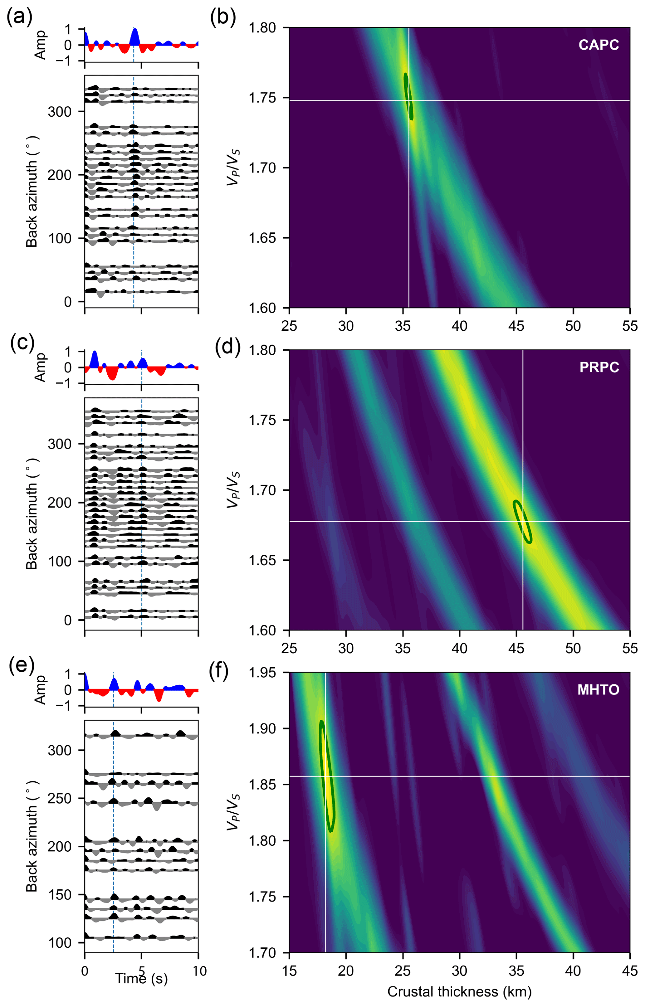
Figure 8 H-k and receiver function estimation for CAPC, STPC and PRCPC stations. (a, c, e) RFs of teleseismic earthquakes (black and white) used to obtain the RFs stack (blue and red). (b, d, f) H-k maps highlighting the maximum power corresponding to the optimal crustal thickness.

3.3 Shear velocity model

We build a 3D shear-wave velocity model on a $\mathrm{0.5}{}^{\circ }\times \mathrm{0.5}{}^{\circ }$ grid with depth increments of 0.5 km from the 1D models obtained from the joint inversion of the phase and group velocities and the receiver functions. We focus on the region between 68–61^∘ W and 6–14.0^∘ N, corresponding to the area in which the highest density of surface-wave velocity and Moho depth estimates is available and well constrained. For each grid point, we invert the phase and group dispersion curves of Rayleigh and Love waves from 10 to 40 s periods in addition to the receiver function corresponding to the nearest station. We allow a maximum distance to a grid point of 0.5^∘ for the RFs, but we do not apply additional weights to the receiver function data according to the distance from the grid point to the nearest station.

Figure 9 shows an example from a location in the Guiana Shield (7.0^∘ N, 65.0^∘ W) of the results obtained from the 1D joint inversion of RFs and Rayleigh- and Love-wave phase and group velocity data. Specifically, the left panels (Fig. 9a) contain the assembled shear-velocity model obtained after the search of 100 000 possible models in each of the 40 Markov chains. Figure 9b–e display the predicted data from the inversion of phase and group velocity data and uncertainties thereof, while Fig. 9f shows the fit to the isotropic receiver function obtained from the MAPC station. We observe some discrepancy (<2 %) between the different datasets, as evidenced by the difficulty to perfectly fit all the data (taking into consideration that dispersion curves and receiver functions have different sources of noise and sensitivities). However, despite some fitting errors, which cause minor perturbations in the 1D profile, we observe an overall good fit to the dispersion curves and to the RF for each grid point. As expected, stations in the shield have fewer errors than those found in the basins. OBS stations were particularly difficult to fit. Probability plots in two geographic points of the cross-section 64.0^∘ W are shown as examples of the inversion results (Fig. S1).

We also present a V_s Moho depth map (Fig. S12) obtained through the Moho depth estimation (manually picked) from the V_s 1D models and the posterior interpolation to the rest of the region of study. The two different Moho maps (Figs. 7 and S12) overall agree well, only with some small differences. It is expected that the results from both observations do not match exactly, as there is an intrinsic tradeoff in the joint inversion, with the different datasets “competing” for the better fit.

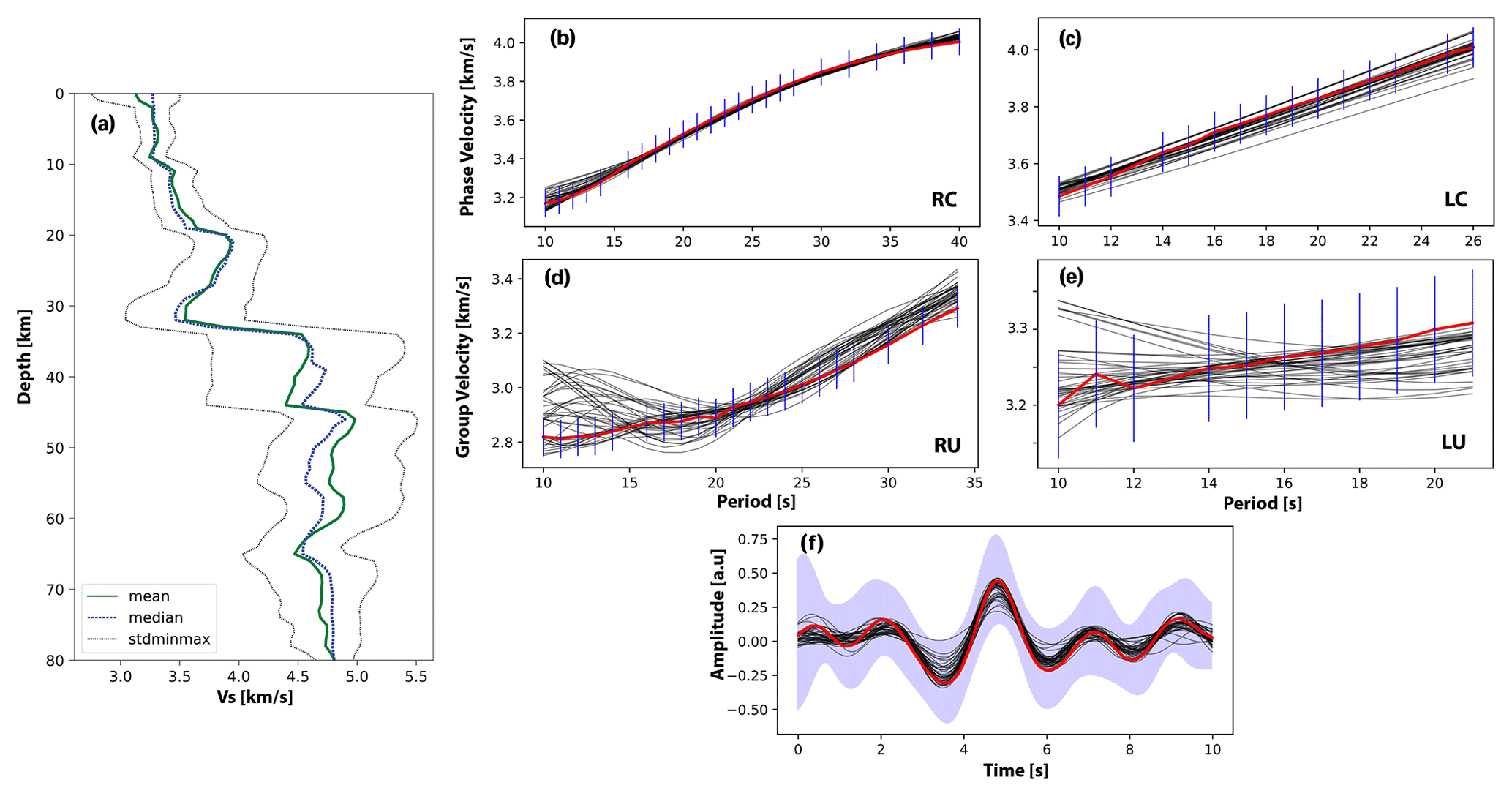
Figure 9 Illustrative example of 1D shear-wave velocity inversion. (a) The green line represents the mean, the blue dots the median and the gray lines the standard deviation estimated for the 1D shear-wave velocity model at 7.0 ^∘ N, 65.0^∘ W (corresponding to the Guiana Shield), from the ensemble of the best models per chain. (b, d) Phase and group velocity fit (gray line is the fit per chain) of the Rayleigh wave; (c, e) phase and group velocity fit of the Love-wave; (f) receiver function of the MAPC station, which was used to do the 1D shear-wave inversion. The red line is the observed dispersion curves and receiver function, blue bars correspond to an error of 3 standard deviations, and the purple shadow is the associated error of the receiver function.

Figure 10 shows un-smoothed horizontal slices of our shear-wave velocity model at different depths ranging from 7.5 to 60 km. We also display uncertainty maps of our joint inversion, corresponding to 1 standard deviation of the mean MCMC joint inversion result, extrapolated for each 1D grid point model (Fig. S13). Furthermore, we include maps comparing the horizontal slices of the 3D model, made of MCMC joint inversion results across all 1D grid points with robust data, with the reference global model ak-135-f (Kennett et al., 1995) (Fig. S14).

To further explore our results with depth we include a set of south-to-north- and west-to-north-oriented depth cross-sections of the model at different longitudes between 61–68^∘ W and 6–14^∘ N in Fig. 11. In the shallower layers of the shear-velocity model (≈15 km), we observe sharp velocity variations and a clear contrast between the Venezuela Basin with low absolute shear velocities and the Guiana Shield with high shear velocities, which is expected for a continental craton. In the Guiana Shield area (Fig. 10a), we observe near-surface faster shear velocities. On the other hand, one of the most remarkable features we see in the cross-sections (66–62^∘ W) is the presence of a slightly low-velocity anomaly from 9–14^∘ N between 8 and 16 km depth, being the strongest in the 64^∘ W cross-section (Fig. 11; B-B^′).

We observe a high-shear-velocity structure through intermediate depth slices of our modeled results (15 to 45 km depth) below the limited area surrounded by Tortuga Island–Barcelona Bay and Margarita Island (Fig. 10b–f). This high-velocity structure persists up to approximately 45 km depth and is also prominent in the cross-sections (Fig. 11d–f) from 64 to 66^∘ W. The deepest parts of our model do not show any remarkable features except for a persistent high-velocity anomaly in the Barcelona Bay that extends towards the southeast beneath the Maturín Basin. In general, we find that shear-wave velocities increase with increasing depth for all regions, with no remarkable velocity inversions. Model cross-sections depict relatively constant Moho depths between 8 and 12^∘ N across the study area, with an interesting dipping structure at around 10^∘ N, suggesting a thickened crust towards the south. Additionally, we see low velocities corresponding to the thick Maturín Basin at 10^∘ N.

Finally, similar to the results of Arnaiz-Rodríguez et al. (2021), we also detect an anomalous low velocity in the lithospheric mantle beneath the Peninsula of Paria that expands from 15 to 22 km depth.

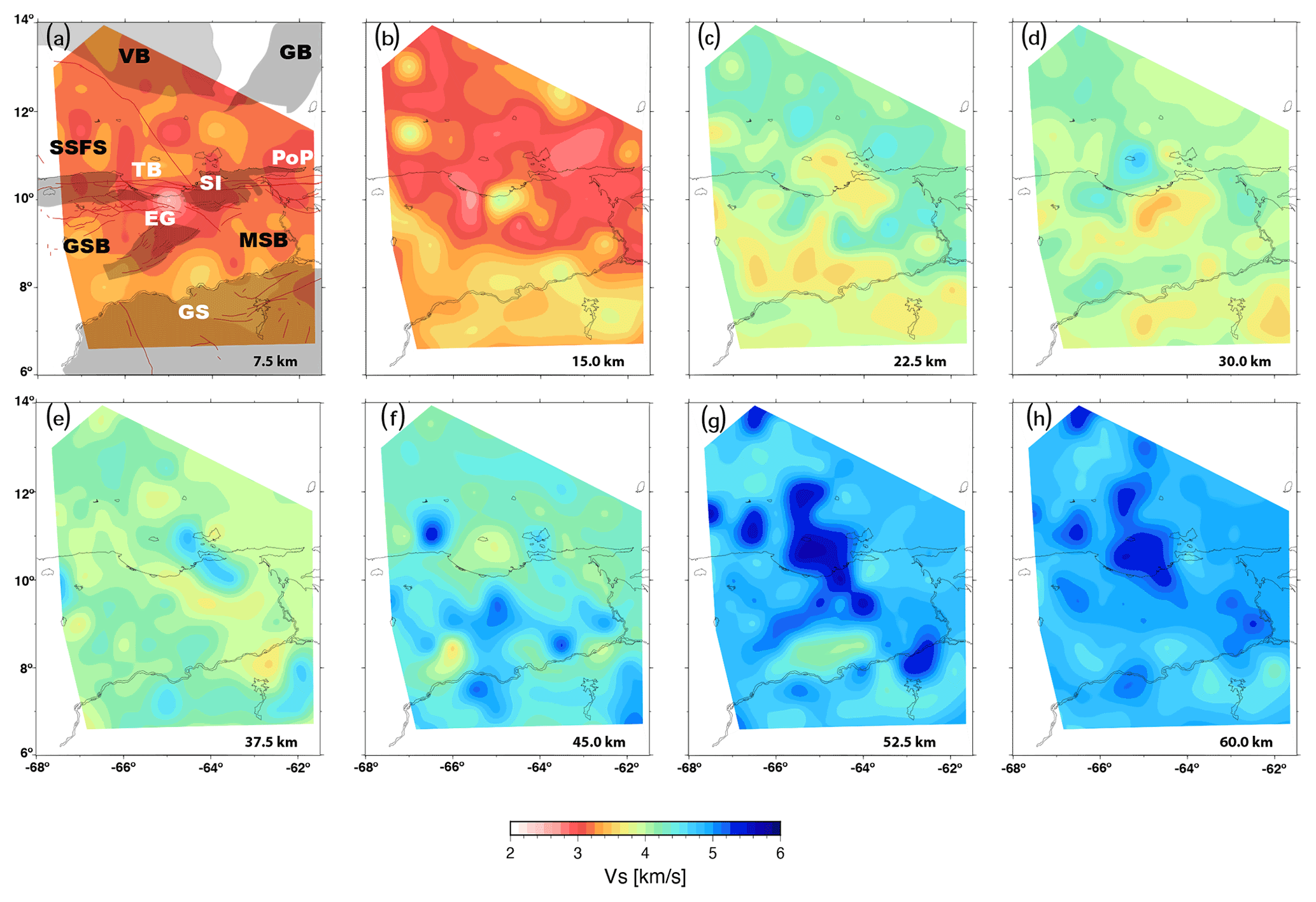
Figure 10 Horizontal slices of the 3D shear-wave velocity model obtained in this study. (a–h) Increasing depth in steps of 7.5 km until 60 km depth. In red we show active faults as presented by Audemard et al. (2006). Abbreviations are VB (Venezuela Basin), GS (Guiana Shield), MSB (Maturín sub-basin), GSB (Guarico sub-basin), SI (Serrania del Interior), EG (Espino Graben), TB (Turtle Island–Barcelona Bay), PoP (Peninsula of Paria) and SSFS (San Sebastian Fault System). VB, GB, SSFS, EG, SI, PoP and GS regions are highlighted with shaded areas.

4 Discussion

Vertically and horizontally polarized dispersion measurements from ambient noise records and teleseismic receiver functions enabled us to investigate the variations in crustal thickness, seismic velocities and Poisson's ratio in northeastern Venezuela. Robust velocity values and anomalies (Figs. 10, 11 and S13), as well as detailed Moho (Fig. 7a) and $V_{\text{p}}/V_{\text{s}}$ maps (Fig. 7b), allow us to image the region in a clearer way than in previous studies (e.g., Niu et al., 2007; Schmitz et al., 2008; Miller et al., 2009; Bezada et al., 2010; Clark et al., 2008; Arnaiz-Rodríguez et al., 2021; Schmitz et al., 2021). For the first time, we image the upper lithosphere using a joint inversion of dispersion measurements and RFs with a robust non-linear inversion. Our results are correlated to well-known geological structures and tectonic provinces and shed new insight into the crustal structure of the region. We begin our discussion by looking into the results derived from receiver function analysis, and then we examine the shear-wave model product of the inversion of the dispersion curves.

4.1 Moho depth from receiver functions

The estimated Moho depth in the study area ranges from 10 to 51 km. Shallower Moho depths (<20 km) are clearly associated with the Caribbean Basin in the north, while the transitional crust and inactive volcanic arcs found between the oceanic plateau and the continental shelf are characterized by a Moho depth ranging between 20 and 30 km. Interestingly, the Serranía del Interior mountain range appears in the map within this region in agreement with previous estimations (e.g., Niu et al., 2007) even though no stations were used inside the range in this study.

We find that the Moho depths on the Venezuelan continental shelf range from 30 to 51 km. We find the region with the greatest Moho depths in the southernmost Guárico Basin, with results similar to the values reported by Niu et al. (2007). Notice that this section is not covered by active seismic data (Schmitz et al., 2021, and references therein). However, our results for the area with the thickest crust are counter-intuitive with regard to standard foreland basin configurations, where the depocenter of the basin is associated with the deepest flexure and the deepest Moho (e.g., Watts, 2001). In the eastern Venezuela Basin, the deepest sediments (∼10 km; Feo-Codecido et al., 1984; Di Croce, 1995; Clark et al., 2008; Bezada et al., 2010) are found in the Espino Graben and Maturín sub-basin, located north and northeast of the region with greatest Moho depths. We find the trend and location of the thickest crust are relatively consistent with the location of the contact between the Precambrian basement (i.e., the Guiana Shield extending beneath the sedimentary layers north of the Orinoco River) and the Cambrian basement found between the Espino Graben and the shield (e.g., Feo-Codecido et al., 1984; Di Croce, 1995). We suggest that this indicates that the allochthonous Paleozoic terrains accreted to the north of the Guiana Shield either had a crustal thickness larger than the shield itself or, alternatively, that the accretion process deformed the crust in such a way that now the deepest Moho is found on this contact. Finally in the south, the Guiana Shield region is characterized by Moho depths ranging between 35 and 40 km. The largest values are consistently associated with Imataca Province (3–2.8 Ga, Guriense), while Pastora Province (2.7–2 Ga, pre-Transamazonic) corresponds to a region with the thinnest crust in the shield at an average crustal thickness of 36 km. On the one hand, these results agree with those reported by Niu et al. (2007), and, on the other, they complement the rather “flat” Moho found by Schmitz et al. (2005, 2008, 2021) around the Guri Dam, with a depth ranging from 46 to 47 km.

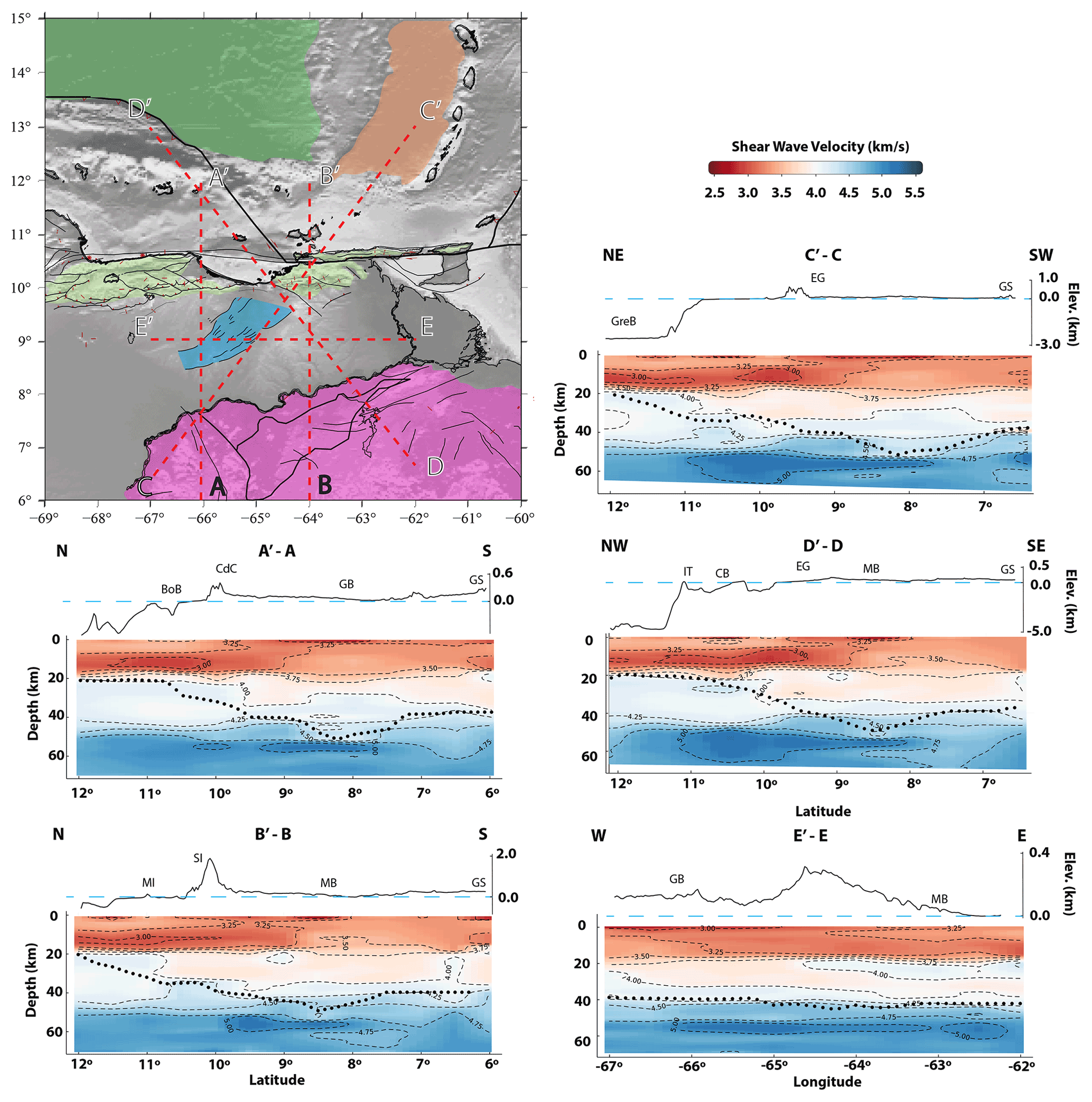
Figure 11 Profiles show the V_s variations across the studied area. On the top left is a map displaying the location of each profile. Each profile shows the V_s structure of the final model and the Moho depth (dotted black line) interpolated with the nearest neighbor algorithm. On the top is the topography and bathymetry from GEBCO 2021 (dashed blue line is 0 m a.s.l.). Contours every 0.25 km s⁻¹. In thin black lines we show active faults as presented by Audemard et al. (2006). Abbreviations are BoB (Bonaire Basin), CdC (Cordillera de la Costa), GB (Guárico Basin), GS (Guiana Shield), MI (Margarita Island), SI (Serranía del Interior), MB (Maturín Basin), IT (Isla La Tortuga), CB (Cariaco Basin), EG (Espino Graben) and GreB (Grenada Basin).

4.2 $V_{\text{p}}/V_{\text{s}}$ Map

Unlike previous attempts (e.g., Niu et al., 2007; Levander et al., 2014), we can consistently map the variations in the average crustal $V_{\text{p}}/V_{\text{s}}$ in the region. In the shield we found an average value of ∼1.72 $V_{\text{p}}/V_{\text{s}}$ (Poisson's ratio of roughly 0.26), consistent with the global average for continental crust (Christensen and Mooney, 1995). Similar to Niu et al. (2007), we find this value to be lower than expected for ancient shields (e.g., Zandt and Ammon, 1995). Niu et al. (2007) attempted to explain this anomaly by suggesting that the crust in the region presents low quantities of granulite-facies mafic rocks. Unfortunately, mafic rocks are rather common in the Imataca (Dougan, 1977) and Pastora (Ostos et al., 2005) provinces. Rather, we propose that the presence of low $V_{\text{p}}/V_{\text{s}}$ can be attributed to the relatively large amounts of quartz in the upper crust in this area, which is consistent with the commonly reported felsic volcanism across the region. Lower values of $V_{\text{p}}/V_{\text{s}}$ (<1.65) are found in the Espino Graben and Peninsula of Paria. In both regions mafic rocks have been reported as (a) basaltic layers found inside the Espino Graben (e.g., Feo-Codecido et al., 1984) and (b) the dacitic rocks (porphyritic rhyolite; Alvarado, 2005) found in the Serranía del Interior. Our results appear inconsistent with the lithology of the regions, suggesting the values are most likely related to the high density of faults in both areas.

4.3 S-wave velocity model

The shear-wave velocity structure of the eastern Venezuelan crust and upper mantle behaves consistently with what is expected for the region. Lower velocities are found at the top of the cross-sections (Fig. 11), gradually increasing with depth, with different trends associated with each of the four main terrains: (a) the Caribbean in the north, (b) the heavily faulted and deformed strike-slip-dominated plated boundary, (c) the foreland basin, and (d) the Guiana Shield in the south. Mean crustal shear-wave velocities (V_s) found in the continental shelf are around 3.99 km s⁻¹ with a standard deviation of 0.64 km s⁻¹, which is higher than the global average (∼3.71 km s⁻¹ according to Laske et al., 2013). The average crustal values for the oceanic region are approximately 3.57 km s⁻¹ with a standard deviation of 0.56 km s⁻¹, also slightly higher than the world's crustal average (∼3.38 km s⁻¹ according to Laske et al., 2013).

At shallow depths (7.5–15.0 km; Fig. 10a, b) our model shows higher V_s values in the Guiana Shield (mean of ∼3.6 km s⁻¹) and lower values in the foreland basin (mean of ∼3.10 km s⁻¹). We note that the higher V_s of the Guiana Shield extends north of the Orinoco River in agreement with results obtained from well perforations (e.g., Feo-Codecido et al., 1984). Lower V_s values found north of latitude 9^∘ N correspond to the foredeeps and depocenters of the basins that reach more than 10 km depth (Feo-Codecido et al., 1984; Di Croce, 1995; Jácome et al., 2003; Clark et al., 2008; Bezada et al., 2010). We also found a low-velocity anomaly beneath the Espino Graben (∼8 km depth), most likely associated with the large number of faults and thick sedimentary layers therein. A similar anomaly appears in the 10 km depth slice (7.5 km; Fig. 10a, b), except for the appearance of a previously unreported high-velocity anomaly within the graben, this anomaly being well resolved in our model (see also Figs. S8 and S9 for detailed checkerboard tests). We suggest that this may be the seismic expression of basaltic intrusions at upper crustal levels that mark the opening of the graben and the intrusion of mafic magmas into the continental crust during the Jurassic (162 ± 8 ma; Feo-Codecido et al., 1984).

At the bottom of the upper crust (∼25 km according to Clark et al., 2008) around 22.5 km (Fig. 10c, d) the Guiana Shield appears rather homogenous, with an average V_s of ∼3.6 km s⁻¹. At this depth our model shows V_s variations that correlate well with differences in age of the different geological provinces in the basement of the eastern Maturín sub-basin. The Precambrian terrains of what was once known as “the Piarra block”, a large area of uplifted Precambrian basement that occupies the Maturín Basin (Feo-Codecido et al., 1984), show higher V_s than the Cambrian allochthonous terrains beneath the Guarico Basin. Hence the petrology of these terrains is likely dissimilar. At 30 to 37.5 km depth (Fig. 10d, e) we see the most prominent anomaly to be the low velocity channel that perfectly aligns with the major faults of the Espino Graben, congruent with the finding of Arnaiz-Rodríguez et al. (2021). Although high-faulting regions appear as a low-S-wave-velocity region (e.g., Yudistira et al., 2017), it is unlikely that faulting is present at lower (ductile) crustal depths. Here, the original thinned/stretched crust (remnant of the Jurassic opening of the graben) has, most likely, been erased by more recent tectonics leaving a deformed and rheologically weakened lower crust that appears in our results as a low-velocity zone. At this depth we also find a dichotomy within the uppermost mantle of the Caribbean basins, with relatively higher V_s values (∼4.2 km s⁻¹) beneath the Venezuela Basin, whereas the Grenada Basin is associated with lower V_s (∼3.9 km s⁻¹). These variations reflect the different histories of both basins: while the Venezuela Basin is a thickened remnant of the original Jurassic Caribbean crust (e.g., Ghosh et al., 1984; Diebold et al., 1999), the Grenada Basin is a back-arc basin that opened due to slab roll-back during the Paleocene (e.g., Arnaiz-Rodríguez and Audemard, 2018). From our tomography model alone, it is not possible to distinguish if the observed anomalies are related to the chemical differences or if the mantle beneath the younger basin is hotter in comparison to that of the older one. Both anomalies can be observed in the model by Arnaiz-Rodríguez et al. (2021).

The lower crust (from 30 to 50 km depth) appears rather homogeneous, with small localized heterogeneities (with a length scale of about 7.5 km; Fig. 10d–g). One feature that stands out is the U-shaped anomaly that aligns with the Urica strike-slip fault and the Pirital frontal thrust (south of the Serranía del Interior; e.g., Audemard et al., 2006). This anomaly implies that the faults extend deep into the crust and represent a major crustal limit. Finally, the uppermost mantle beneath the continental shelf shows a large high-velocity anomaly (deviation of ∼20 %; see Fig. S14). Part of this anomaly again follows the general trend of the Espino Graben, perhaps a testament to the anatexis produced by the lithospheric thinning driven by the opening of the Espino Graben. The largest anomaly, found west of the Peninsula of Paria, largely disagrees with a low-velocity anomaly found by Miller et al. (2009) in the same region but agrees with another high-velocity anomaly reported by Arnaiz-Rodríguez et al. (2021). This anomaly is not related to any known feature in the region and could represent a chemically anomalous region in the upper mantle, so it is perhaps a remnant of the southernmost prolongation of the Antilles subduction beneath South America (e.g., VanDecar et al., 2003; Bezada et al., 2010).

We present a detailed picture of the crustal structure across four profiles (Fig. 11) containing shear-wave velocity variations as well as the Moho depth. The first profile (A-A^′), along −66^∘ W, shows, for the first time, the crustal structure beneath Cuchivero Province, with an upper crustal layer of ∼20 km and with a homogeneous lower crust. The lower mantle in this section appears with a smooth velocity gradient increasing from 4.25 km s⁻¹ (at the Moho) to 4.75 km s⁻¹ at 60 km depth. North of the Orinoco River, the crust thickens from 40 to 50 km, with the maximum depth coinciding with the position of the Altamira Fault (the physical limit between the southern Precambrian terranes and the northern Paleozoic ones) reported by Feo-Codecido et al. (1984). The crust in this area appears well differentiated into four layers: an upper crust of ∼20 km, a thin middle crust (thickness <10 km) and two lower crustal layers with high velocity when compared to the global average for continents of ∼3.93 km s⁻¹ (Laske et al., 2013). When compared to the simpler crust found in the south of our study region, we find increasing evidence of the collision and thickening of the crust and suture of two blocks during the emplacement of the Paleozoic terranes to the Guyana Shield. Further to the north, V_s in the upper crust decreases near the Cordillera de la Costa range, where low V_p velocities were also reported via wide-angle seismic profiling (Magnani et al., 2009). Most likely, this represents the nappe systems formed from the Paleocene to the Eocene by the collision of the Caribbean arc with northern South America. Here, the Moho gradually thins out up to the San Sebastian Fault System, which separates the extended transitional crust (originally an arc) from the continental platform (Passalacqua et al., 1995). Finally, in the northernmost section of the profile, we find a thick crust beneath the Bonaire Basin, similar to the values reported by Bezada et al. (2010).

The second profile (B-B^′) shows a similar structure, but we highlight a few important differences. Firstly, we find possible evidence of intrusions and chemical heterogeneities at the base of the crust of the Guyana Shield, in agreement with geological observations that report intrusions of different types of igneous rocks (from granitic to ultramafic) and greenstone belts rocks (Sidder, 1990) that commonly occur in Imataca Province. On this profile, the maximum Moho depth does not correspond with any known structure but could reflect the prolongation to the east of the feature reported in profile A-A^′. North, towards the Serranía del Interior and Margarita Island, the Moho is mostly constant within the contour of 4.25 km s⁻¹, but this changes due to a lack of data further north, where the Moho beneath the transitional crust is better defined by the V_s model than by the interpolation of the receiver function data. Interestingly, this profile shows a high-velocity anomaly and small shortening in the continental crust beneath the Serranía del Interior and the Maturín Basin that could be consistent with a NE projection of the Espino Graben (e.g., Sanchez et al., 2011). Previously these features have only been ineffectively found through heavily processed aeromagnetic data interpretation (e.g., Gonzalez et al., 2017), and in our model they have been found thanks to the combined analysis of the Moho depth, RFs and dispersion measurements.

The Espino Graben structure is better appreciated in profiles C-C^′ (along the axis of the graben) and D-D^′ (perpendicular to the structure). Low-velocity anomalies are reported along the structure, as well as crustal thinning, a remnant of the opening of the graben. Also, high-velocity anomalies can be appreciated in the lower crust in profiles B-B^′, C-C^′ and D-D^′, most likely revealing the inclusion of mafic material during the extension process that created the Espino Graben. Most of the anomalies seem to have some smearing to the north, but as the graben area is well covered (Figs. S7 and S8, which show resolution maps) this is unlikely to be produced by limitations in ray-path coverage (see also Figs. S2–S5, which show good resolution in this region). Therefore, we suggest that the master fault of the graben deepens to the north, corroborating previous findings from Arnaiz-Rodríguez et al. (2021). As high-velocity anomalies consistently appear beneath the graben we cannot disprove the possibility of trapped material within the lithospheric mantle, which is a hallmark of the process disproved above. Moreover, in profile D-D^′ we also see the crustal structure beneath Pastora Province that clearly shows a differentiation in upper, middle and lower crust.

Profile E-E^′ (in the W–E direction) shows the crustal difference between the two sub-basins that compose the eastern Venezuela Basin. Geologists have long tried to establish the difference between both, and in general the most important difference is that the Guárico Basin (to the west) sits on top of a Paleozoic age, while the Maturín one (to the east) formed over a Precambrian basin (the Piarra block, after Feo-Codecido et al., 1984) where granite was found below the sediments at 4.3 km depth. Here, we show that the upper crust–lower crust transition zone and the Moho appear to be rather flat (as would be expected for an along-the-structure profile in a foreland basin). We find that the main difference is a large high-velocity layer in the lower crust beneath the Maturín Basin. This kind of anomaly is similar to those found at the southern end of profiles A-A^′ and B-B^′, reinforcing the long-lasting geological interpretation that the Precambrian layers of the shield extend to the north beneath the eastern section of the basin (e.g., Yoris and Ostos, 1997).

5 Conclusions

We present a new, 3D shear-wave velocity model of the SE Caribbean area built from a dense set of 1D models (spaced in a $\mathrm{0.5}{}^{\circ }\times \mathrm{0.5}{}^{\circ }$ grid). The 1D models were obtained from a non-linear joint inversion of phase and group velocities of surface waves and receiver functions, using a Markov chain Monte Carlo algorithm (Dreiling et al., 2020). Additionally, we provide a new Moho depth map obtained from a semblance-weighted H-k stacking analysis of receiver functions, which shows remarkable tectonic features. From the interpretation of these results, we outline the following conclusions.

The Moho interface in the region ranges from 10 to 51 km. Values <20 km are associated with the Caribbean crust, the transitional crust ranges between 20 and 30 km, and the Venezuelan continental shelf ranges from 30 to 51 km. A small shortening in the continental crust is reported inside the Espino Graben, a testament to the opening of the graben. A thickening of the crust, north of the Orinoco River, seems to be closely associated with the collision between Precambrian and Paleozoic basement blocks. This indicates that the collision and subsequent suture thickened the crust, and this structure is now buried beneath the sediment of the foreland basin.

The crust of the Guiana Shield is drastically heterogeneous. Variations are related to each of the major tectonic provinces therein. From west to east, we find that (a) Cuchivero Province presents an upper crustal layer and a homogeneous lower crust; (b) Imataca Province shows a similar upper crust to Cuchivero Province but a heterogeneous lower one with anomalies possibly related to intrusions at the base of the crust; and (c) Pastora Province appears to show a differentiated section divided into upper, middle and lower crust.

The Espino Graben is associated with low values of V_s in the sedimentary layers (<3.0 km s⁻¹) and in the upper crust (<3.5 km s⁻¹), which are related to the large number of faults in the region. Furthermore, we find several high-velocity anomalies between 10 and 15 km and between 20 and 25 km (>4.0 km s⁻¹). These are likely related to the basaltic rocks that intruded the crust during the opening of the graben in the Late Jurassic.

We report high-velocity bodies as well as a thinner crust beneath the Espino Graben, remnants of the extension that formed the structure. Furthermore, we found the first seismological evidence that the graben extends beneath the Serranía del Interior range.

The V_s in the upper mantle of the Caribbean Basin in the region is drastically different: ∼4.2 km s⁻¹ at the Venezuela Basin and ∼3.9 km s⁻¹ at the Grenada Basin. This difference arises from the different age (old and cold lithospheric keel should have a larger V_s) and geological history.