the Creative Commons Attribution 4.0 License.
the Creative Commons Attribution 4.0 License.
 | 10 Feb 2022
Seismic monitoring of the STIMTEC hydraulic stimulation experiment in anisotropic metamorphic gneiss
Carolin M. Boese
Grzegorz Kwiatek
Thomas Fischer
Katrin Plenkers
Juliane Starke
Felix Blümle
Christoph Janssen
Georg Dresen
In 2018 and 2019, we performed STIMulation tests with characterising periodic pumping tests and high-resolution seismic monitoring for improving prognosis models and real-time monitoring TEChnologies for the creation of hydraulic conduits in crystalline rocks (STIMTEC). The STIMTEC underground research laboratory is located at 130 m depth in the Reiche Zeche mine in Freiberg, Germany. The experiment was designed to investigate the rock damage resulting from hydraulic stimulation and to link seismic activity and enhancement of hydraulic properties in strongly foliated metamorphic gneiss. We present results from active and passive seismic monitoring prior to and during hydraulic stimulations. We characterise the structural anisotropy and heterogeneity of the reservoir rocks at the STIMTEC site and the induced high-frequency (>1 kHz) acoustic emission (AE) activity, associated with brittle deformation at the centimetre-to-decimetre scale. We derived the best velocity model per recording station from over 300 active ultrasonic transmission measurements for high-accuracy AE event location. The average P-wave anisotropy is 12 %, in agreement with values derived from laboratory tests on core material. We use a 16-station seismic monitoring network comprising AE sensors, accelerometers, one broadband sensor and one AE hydrophone. All instrumentation was removable, providing us with the flexibility to use existing boreholes for multiple purposes. This approach also allowed for optimising the (near)-real-time passive monitoring system during the experiment. To locate AE events, we tested the effect of different velocity models and inferred their location accuracy. Based on the known active ultrasonic transmission measurement points, we obtained an average relocation error of 0.26±0.06 m where the AE events occurred using a transverse isotropic velocity model per station. The uncertainty resulting from using a simplified velocity model increased to 0.5–2.6 m, depending on whether anisotropy was considered or not. Structural heterogeneity overprints anisotropy of the host rock and has a significant influence on velocity and attenuation, with up to 4 % and up to 50 % decrease on velocity and wave amplitude, respectively. Significant variations in seismic responses to stimulation were observed ranging from abundant AE events (several thousand per stimulated interval) to no activity with breakdown pressure values ranging between 6.4 and 15.6 MPa. Low-frequency seismic signals with varying amplitudes were observed for all stimulated intervals that are more correlated with the injection flow rate rather than the pressure curve. We discuss the observations from STIMTEC in context of similar experiments performed in underground research facilities to highlight the effect of small-scale rock, stress and structural heterogeneity and/or anisotropy observed at the decametre scale. The reservoir complexity at this scale supports our conclusion that field-scale experiments benefit from high-sensitivity, wide-bandwidth instrumentation and flexible monitoring approaches to adapt to unexpected challenges during all stages of the experiment.
- Article
(9972 KB) - Full-text XML
-
Supplement
(2517 KB) - BibTeX
- EndNote


Mesoscale in situ hydraulic stimulation experiments performed in well-instrumented underground research laboratories (URLs) offer a number of advantages over small-scale laboratory tests and reservoir-scale experiments. In particular, URL experiments capture structural heterogeneity on a realistic length scale and are thus essential to transfer results from laboratory tests on centimetre-scale rock samples to reservoir rocks at the kilometre scale (Young et al., 2000; Gischig et al., 2019). Furthermore, URL experiments allow for validation of inferred results, e.g. through mine-back drilling into stimulated rock volumes (e.g. Warren and Smith, 1985). Most importantly, intermediate-scale in situ experiments, conducted in URLs, allow for a close to optimal placement of seismic sensor networks for monitoring and characterisation of the target volume (Ohtsu, 1991; Zang et al., 2017; Amann et al., 2018; Kwiatek et al., 2018; De Barros et al., 2019; Feng et al., 2019). Hydraulic stimulation was seismically monitored during in situ experiments in various settings (e.g. Ohtsu, 1991; Dahm et al., 1999). The monitoring systems need to be tuned to the seismic waves associated with hydraulic stimulation in terms of sensitivity, frequency range and attenuation characteristics of the rock, which limit the detection ranges of the seismic signals (e.g. Mendecki et al., 1999; Plenkers et al., 2010, 2011; Manthei and Plenkers, 2018). Varying noise conditions on site often impact monitoring conditions (Plenkers et al., 2010, 2013). Recently, monitoring of a hydraulic stimulation experiment at 410 m depth at the Äspö Hard Rock Laboratory (AHRL) in southern Sweden in May–June 2015 (Zang et al., 2017; Kwiatek et al., 2018) showed that only two of the multiple seismic monitoring systems in place were suitable to record the observed seismic processes. The high-sensitivity acoustic emission (AE) network recorded high-frequency (>1 kHz) AE events from fracturing and frictional sliding with rupture dimensions on the centimetre to decimetre scale. A five-station broadband network recorded low-frequency signals of 0.004–0.008 Hz during the frac and refracs. Slow deformation processes have also been monitored with tilt sensors during the “In-situ Stimulation and Circulation Experiment” performed at Grimsel Test Site (GTS) in Switzerland. This experiment was conducted at a depth of 480 m below surface, within an experimental volume of approximately 20 m × 20 m × 20 m of granitic rock between February and May 2017 (Gischig et al., 2018). Dense 3-D coverage and the close proximity of seismic instrumentation to induced AE events both at the AHRL and the GTS sites resulted in high-quality datasets resolving details of the hydromechanical processes on the decimetre-to-metre scale (e.g. Dutler et al., 2019; Kwiatek et al., 2018; Villiger et al., 2020; Niemz et al., 2020). This level of detail is necessary to advance our understanding of processes relevant for hydraulic stimulations such as (1) hydromechanically coupled fluid flow and pore pressure propagation, (2) transient pressure-dependent and permanent slip-dependent permeability changes, (3) fracture formation and interaction with pre-existing structures, (4) rock-mass deformation around the stimulated volume due to fault slip, failure processes and poroelastic effects and (5) the transition from aseismic to seismic slip (Amann et al., 2018). AE event distributions can provide detailed information on the small-scale spatiotemporal evolution of the deformation within the reservoir induced by hydraulic stimulation. In particular, fracture dimensions, orientations, faulting style and the orientation of the prevailing principal stress axes may be inferred from the analysis of induced seismic events (Manthei et al., 2001; van der Baan et al., 2013; Manthei and Plenkers, 2018; Krietsch et al., 2019).
We performed STIMulation tests with characterising periodic pumping tests and high-resolution seismic monitoring for improving prognosis models and real-time monitoring TEChnologies for the creation of hydraulic conduits in crystalline rocks (STIMTEC) to develop diagnostic criteria for successful hydraulic stimulations and to optimise monitoring and stimulation procedures. This experiment was conducted in strongly foliated and heterogeneous metamorphic rock at shallow depth (∼ 130 m). Complementary to the STIMTEC experiment, several other mesoscale injection experiments in crystalline rock are currently underway. The “EGS Collab Experiment” is a multi-institutional collaborative research project at a similar scale that aims to solve technological problems related to reservoir creation and operation of enhanced geothermal systems (EGSs) through different stimulation procedures under realistic in situ stress conditions and to provide a test bed for the validation of existing thermal–hydrological–mechanical–chemical numerical modelling tools (Kneafsey et al., 2018). The second experimental phase is currently planned at the Sanford Underground Research Facility (SURF) at 1.25 km below surface, located in the Homestake Mine, a former gold mine in South Dakota, USA (Kneafsey and the EGS Collab Team, 2020). The Bedretto experiment aims at upscaling previous mesoscale experiments by a factor of 10 (Gischig et al., 2019) and is located in the Bedretto Underground Laboratory for Geoenergy research (BULG) in southern Switzerland, about 10 km southeast of the GTS. Current activities aim at stimulating the Rotondo granite at the Bedretto tunnel with an overburden about 1 km thick in an estimated volume of approximately 300 m × 100 m × 50 m allowing to test different hydraulic stimulation as well as seismic and deformation monitoring techniques.
Site complexity due to small-scale rock stress and structural heterogeneity and/or anisotropy of varying strength and orientation is a major issue encountered by all mesoscale in situ experiments so far. To trace the spatiotemporal evolution of AE events during hydraulic stimulations at high resolution, the accuracy of the applied seismic velocity model for location in anisotropic and heterogeneous rock volumes is of fundamental importance. At the laboratory scale, anisotropic velocity models are commonly applied (e.g. Stanchits et al., 2003) to monitor rock deformation at high resolution. At the mine scale, comprehensive and dense in situ measurements, in particular active seismic surveys, are performed to characterise heterogeneity and anisotropy of the investigated rock volume. These seismic surveys are commonly performed prior to a stimulation to derive the velocity structure and repeatedly in material science and in situ experiments to monitor alteration of the rock volume, e.g. by fracture generation. Repeated active measurements throughout hydraulic stimulation experiment are still scarce. Their value for monitoring temporal changes resulting from fluid pressure changes in the rock volume has only recently been recognised (Doetsch et al., 2018; Rivet et al., 2016; Schopper et al., 2020). At the field scale, detailed site characterisation is often not possible because of associated costs and limited placement of instrumentation, resulting in velocity model ambiguity and lower resolution of the seismic event distribution. Thus, in STIMTEC, we performed resolution tests at the mesoscale to place better constraints on model uncertainties and to provide estimates of the effect of simplifications and approximations required at the field scale.
The seismic response to stimulation during recent URL experiments was highly variable. At the AHRL site, seismic response to stimulation likely depended on rock type with granodiorite and granite stimulations showing seismicity in contrast to diorite–gabbro host rocks. However, this interpretation is complicated by the fact that three different fluid-injection schemes were applied to test their influence on injectivity and induced seismicity (Zang et al., 2013; Niemz et al., 2020). At the GTS site, two shear zones (S1, S3) with different deformation histories in the Grimsel granodiorite were stimulated. Hydrofrac experiments revealed remarkably different seismic responses north and south of the S3 shear zone in terms of injection pressure, amount of backflow, injectivity before jacking and final transmissivity (cf. Figs. 4 and 5 of Dutler et al., 2019). Villiger et al. (2020) observed differences in the seismicity patterns observed during hydroshear stimulation of the two shear zones. During stimulation of the S1 shear zones, the majority of AE events occurred at the beginning of injection, when the total volume of injected fluid was low, whereas for the S3 shear zone the number of AE events increased with the volume of injected fluid (Villiger et al., 2020). Hydroshear stimulations of the ductile S1 shear zone showed less seismicity overall and larger transmissivity increases than S3 hydroshear stimulations. The seismic responses to stimulation during the EGS Collab Experiment were also complex (Schoenball et al., 2020; Fu et al., 2021). Abundant seismicity accompanied the three hydraulic stimulations at 1.5 km depth at SURF aiming to establish a connection between injection and production boreholes approximately 10 m apart (Kneafsey et al., 2019). Seismicity delineated at least 10 planar features with variable orientations that connected to an open natural fracture, which formed a significant fluid pathway and controlled the stimulations (Schoenball et al., 2020; Fu et al., 2021).
Here, we introduce the STIMTEC project, its monitoring concept and lessons learned from using a 16-station seismic monitoring network for active and passive seismic monitoring during a decimetre-scale hydraulic stimulation experiment in anisotropic and heterogeneous rock. We compare our monitoring experience with other previous and ongoing research experiments in URLs. We review our seismic monitoring strategy, monitoring system adjustments and discuss potential applications to the field scale. We address how anisotropy and heterogeneity are characterised and provide estimates to place better constraints on the effect resulting from simplifications and approximations commonly applied at the field scale.
2.1 Objectives, experimental framework and monitoring strategy
The STIMTEC experiment focuses on the development and optimisation of hydraulic stimulation and aims at establishing the link between damage patterns, hydraulic properties and observed seismic activity to provide diagnostic criteria for the success of a stimulation (Renner and STIMTEC team, 2021). Therefore, seismic and hydraulic monitoring are key components of the experiment. In addition, validation through mine-back drilling into stimulated volumes of complex rock, small-scale laboratory tests to characterise mechanical and physical properties and numerical modelling are part of the integrated project approach.
The STIMTEC experiment comprised the following phases:
-
a pre-stimulation characterisation phase (including site characterisation, borehole drilling and logging, core analysis and hydraulic measurements for interval selection, as well as instrumentation);
-
the stimulation phase (stimulation of 10 selected intervals in the injection borehole during 16–18 July 2018);
-
the hydraulic testing phase (testing of six intervals in the injection borehole during 8–10 August 2018);
-
the validation phase (mine-back drilling of three validation boreholes, stress measurements in five intervals of the vertical validation borehole on 21–22 August 2019); and
-
the final hydraulic testing phase (testing of seven intervals in the injection borehole during 5–8 November 2019).
High-resolution seismic monitoring accompanied all experimental phases but with different foci. During the pre-stimulation characterisation phase, active seismic monitoring aimed at identifying high-attenuation and deformation zones to avoid sensor installation in these zones, to quantify detection ranges and to obtain a velocity model. The installed sensors were then used to characterise background noise levels and any natural seismicity at the site. During the stimulation phase and subsequent validation phase, real-time passive monitoring aimed at optimised AE event detection, localisation and magnitude estimation during stimulation of intervals in the injection and vertical validation boreholes. Repetitive active seismic measurements were performed along the injection and validation boreholes to investigate any elastic velocity changes resulting from the stimulation. During the final hydraulic testing phase, passive seismic monitoring focused on verifying detection rates observed for some stimulated intervals with few AE events by placing two sensors closer to these intervals.
2.2 Site description and infrastructure
The STIMTEC site is located on the second floor of the Reiche Zeche mine, in the eastern Ore Mountains beneath the city of Freiberg, Germany, at a depth of approximately 130 m below surface (Fig. 1). The metamorphic gneiss complex, hosting the mine, is referred to as the Freiberger gneiss anticline and belongs to the Precambrian metamorphic basement of the internal mid-European Variscan orogen (Seifert and Sandmann, 2006). It hosts silver, lead and zinc ores, which were mined for centuries (Bayer, 1999). Temperatures at the STIMTEC site are low (∼ 10 ∘C). The protolith of the inner grey gneiss at Freiberg likely was an S-type granite (Tichomirowa et al., 2001, and references therein), which was metamorphosed at about 0.8 to 1.1 GPa and 600 to 700 ∘C and has a Proterozoic age with minimum estimates of 548 to 534 Ma (cf. Fig. 11 of Tichomirowa et al., 2001). The fine-grained biotite gneiss has a granitic appearance and often contains large potassium–feldspar porphyroblasts. The mineral composition of Freiberg gneiss is generally characterised by biotite, potassium–feldspar, plagioclase and quartz (Tichomirowa et al., 2001). Freiberg gneiss is a partly weathered, faulted and strongly foliated rock. Large, steeply dipping mineralised fault zones strike through the gneiss (Sebastian, 2013).
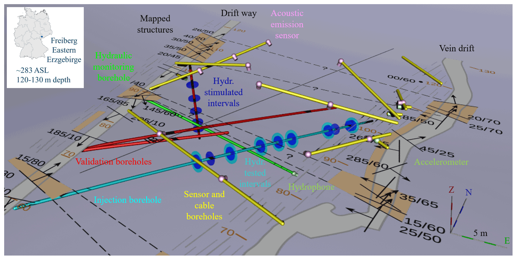
Figure 1Overview of the borehole network and mapped structures along the galleries at the STIMTEC site in the Reiche Zeche mine. The eastern gallery is the curved vein drift; the western gallery is the straight driftway, which is oriented almost north–south. Deformation zones (brown zones) are marked along the galleries and assumed to belong to connected systems between the galleries based on the orientations of mapped structures identified in the pre-characterisation phase of the experiment. The monitoring system comprises 12 acoustic emission piezo sensors (purple) located in horizontal or upward-going seismic monitoring boreholes (yellow). Three accelerometers (light green) are collocated with AE sensors. A broadband sensor was moved from a short horizontal borehole off the vein drift to the vertical validation borehole (red) in driftway during the course of the experiment. An AE hydrophone was placed at the bottom of the hydraulic monitoring borehole (green) for the last hydraulic testing phase of the experiment. Stimulation intervals (dark blue) in the injection borehole (cyan) and the vertical validation borehole (red) are shown together with hydraulically tested intervals (light blue). Inset shows the regional setting of the mine in Freiberg, Germany.
The monitored rock volume at the STIMTEC site has dimensions of 40 m × 50 m × 30 m and is situated between two galleries: the straight driftway and the curved vein drift that tracks the mined ore lode “Wilhelm Stehender” (Fig. 1), a major mineralised fault zone with a thickness of up to 2 m that strikes north and dips westward beneath the site. Large ore lodes at Reiche Zeche are generally considered normal faults and trend predominantly north–south to northeast–southwest. The galleries have a square cross section (width/height of approximately 2 m) and were excavated in 1903 (vein drift) and 1950 (driftway).
In total, 17 boreholes with uniform radius (76 mm) were drilled in two phases. The 11 seismic monitoring boreholes were completed with a range of orientations and lengths, extending horizontally or upwards from the galleries (Fig. 1). The 63 m long injection borehole was drilled with a strike of N31∘E and dip of 15∘ downwards to maximise the inclination angle between the subhorizontal foliation and the injection borehole while fulfilling seismic monitoring requirements (possible recording ranges to upwards directed boreholes, placed outside of damage zones). A more steeply inclined (dipping 36∘, striking N66∘ E) hydraulic monitoring borehole was drilled, extending below the central part of the injection borehole with a minimum distance of 2.5 m between the borehole depth 18.4 m in the hydraulic monitoring borehole and 33.9 m in the injection borehole. One cable borehole, connecting the two galleries, was drilled for cable as well as seismic sensor installations. The validation phase comprised mine-back drilling of two inclined validation boreholes of 19.3 and 45.8 m length, running subparallel to the injection borehole and targeting seismically active and inactive volumes, as well as a vertical borehole for evaluation of the stress field (Fig. 1). The short validation borehole dips ∼ 12∘ and ends 3.5 m above the injection interval 28.1 m in the injection borehole, while the long inclined validation boreholes dips ∼ 15∘, terminating 4.4 m sideways of the injection interval at 56.6 m. The 15.6 m long vertical validation borehole (dip angle of ∼ 89∘) is located in the driftway and spans the same absolute depth range as the injection borehole.
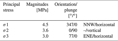
The STIMTEC site is located 180 m south of the GFZ underground laboratory (Giese and Jaksch, 2016), where extensive site investigations and exploration monitoring in the 10–3000 Hz frequency range have been performed over the last 20 years to characterise the rock mass. The excavation damage zone (EDZ) of the galleries at the GFZ lab may extend up to 10 m into the rock volume with an estimated 7 % reduction in P-wave velocity (Krauß et al., 2014). A continuous east–west-trending damage zone was seismically imaged, showing an approximately 13 % P-wave velocity reduction compared to the surrounding rock mass (Krauß et al., 2014). Predominantly east–west-trending structures are likely relicts given their orientation with respect to the current regional stress field. The stress field was measured at 140 m depth in the mine, a few hundred metres from the STIMTEC site using an overcoring technique (Table 1; Mjakischew, 1987), suggesting a strike-slip regime with maximum horizontal compressive stress orientation directed NNW–SSE, which is typical for SE Germany.
Table 1Results of stress measurements through overcoring by Mjakischew (1987) at 140 m depth in the Reiche Zeche mine.
2.3 Structural analyses
Geological structures within the STIMTEC rock volume were identified through mapping of the access galleries, acoustic televiewer images of the injection, hydraulic monitoring and validation boreholes, and from inspection of the recovered core material. This aimed at the detection of possibly continuous fracture systems or damage zones, which could affect the recording of high-frequency acoustic emission events. The foliation was mapped at 34 positions and determined to be subhorizontal to shallowly dipping in a southeast direction. At least two east–west-trending, steeply dipping deformation zones were identified in both galleries that occasionally serve as water conduits as indicated by oxidation and Fe2O3 deposition in the otherwise intact rock mass. These are referred to as the northern and southern deformation zones. A third zone, the “middle deformation zone”, was predominantly seen in the vein drift. Drilling and coring of the injection and validation wells allowed us to check whether these deformation zones actually crossed the entire STIMTEC volume (question marks in Fig. 1). The density of open fractures identified from acoustic logs is highest (with 20 fractures per metre) at the bottom of the injection and long inclined validation boreholes, compared to typical values of five open fractures per metre elsewhere (Adero, 2020). Several prominent structures (at 60 and 62 m) with a range of orientations were identified in the logs from the injection borehole (Fig. 2), where the core becomes severely fractured and was not fully recovered. This zone is considered the continuation of the northern deformation zone at depth within the rock volume. Its location and depth are consistent with the orientation of mapped structures in both galleries (Fig. 1).
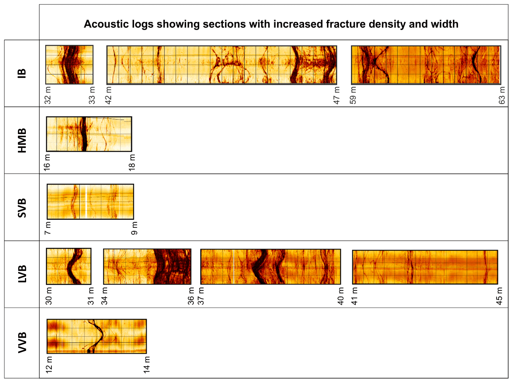
Figure 2Acoustic borehole televiewer logs indicating sections along the boreholes with increased fracture density and width, intercepted by the injection borehole (IB), hydraulic monitoring borehole (HMB), short inclined borehole (SVB), long inclined borehole (LVB) and vertical validation (VVB) borehole. Modified from Adero (2020).
A connection of the middle damage zone between the driftway and the vein drift is not well constrained. A prominent single fracture is mapped at 32.5 m depth in the injection borehole, also seen at 17 m in the hydraulic monitoring borehole and at 19.8 m in the long, inclined validation borehole (Fig. 2). However, this notable structure was not observed in the short, inclined validation borehole. Its interpreted orientation does not match the interpolated position of the middle damage zone based on mapping in the galleries. Ultrasonic transmission measurements from the cable borehole, connecting the two tunnels, indicate that the mapped deformation zone seen in vein drift extends several metres into the rock volume but does not connect to the driftway.
Between 33–41 m depth in the injection borehole, the number of healed fractures identified from the core is largest. Two prominent structures are seen at 46 and 47 m depth, located in a section of the injection borehole (42–50 m) that contains more fractures on average (Fig. 2). The same two structures are likely seen at 38–39 m depth in the long validation borehole.
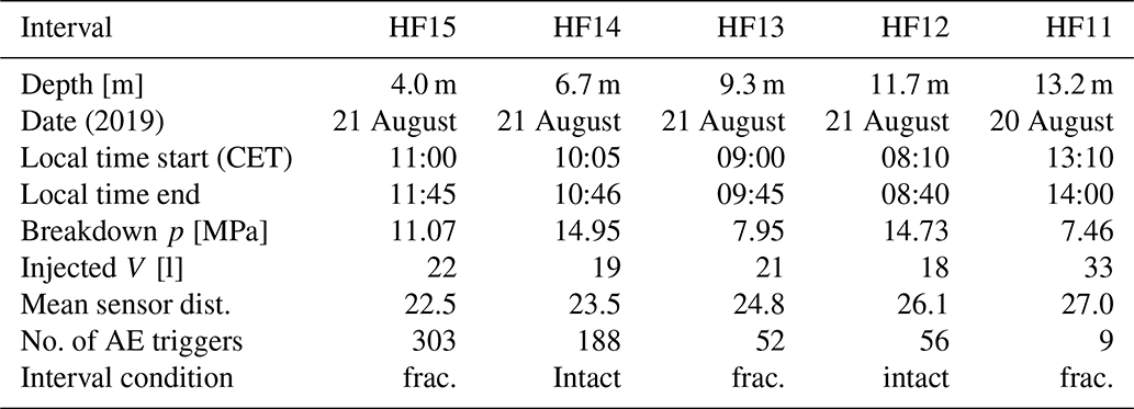
Based on the distribution of fractures obtained from core analyses and acoustic image logs as well as hydraulic pre-characterisation results, 10 stimulation intervals of 0.75 m length each were selected for stimulation in the injection borehole. Intact intervals were located at borehole depths of 22.4, 24.6, 28.1, 33.9 and 37.6 m (depths reference to the position of the middle of the double-packer probe), while intervals with pre-existing fractures were located at 40.6, 49.7, 51.6, 55.7 and 56.5 m depths (Table 2). Four intact sections and one test interval with a pre-existing fracture were selected for stimulation in the vertical validation borehole, corresponding to 4.0, 6.7, 9.3, 11.7 and 13.2 m depths (Fig. 1 and Table 3).
Table 2Overview of stimulation details for the 10 stimulated intervals of the injection borehole. The total injected volume and number of AE events are given for the whole stimulation sequence as shown in Fig. 4. The stimulation intervals were chosen to contain as few pre-existing structures as possible based on cores and acoustic logs. The interval condition was reassessed based on the stimulation results as either intact where hydrofracs were created or pre-fractured, meaning that hydroshearing occurred.
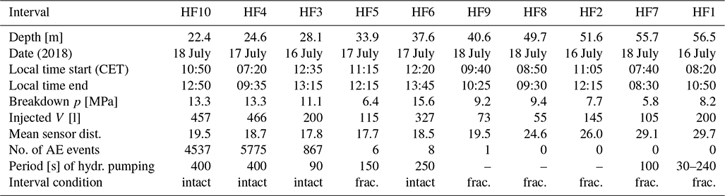
Table 3Minifrac measurement interval details for the vertical validation borehole. See Table 2 for explanation.
2.4 Hydraulic injection scheme
All selected intervals in the injection and vertical validation borehole were stimulated with a uniform fluid-injection scheme: first, a pulse test was performed in the packed-off interval. The test interval was pressurised to assess the performance of the packers and to assess the presence or absence of pre-existing open conductive fractures. Hydraulic properties were obtained from the time that it takes the pressure to decay from the initial pressure to a certain level (Bredehoeft and Papadopulos, 1980; Cooper et al., 1967). Secondly, fluid was injected into the packed-off interval, maintaining a constant flow rate and thereby raising the interval pressure until breakdown to create a hydraulic fracture. Once the breakdown pressure was reached the injection was shut in. Thirdly, three refrac tests were performed at the same flow rate as applied during the initial hydrofrac test to determine fracture reopening pressures, to propagate the fracture and to monitor the evolution of shut-in pressures after each refrac. Subsequently, a step-rate test was performed, comprising stepwise increases of the injected fluid to determine the jacking pressure, when the created fractures changed their state from mechanically closed to mechanically opened. Optionally, a periodic pumping test sequence was performed to derive hydraulic properties, consisting of phases of alternating flow rates between two levels, ranging from to L min−1, for periods varying between 20 and 900 s (∼ 15 min; Table 2).
2.5 Seismic monitoring network and data acquisition
The seismic monitoring network consisted of 16 sensors, installed in boreholes of 1.5 to 20 m length to reach as far as possible into or beyond the tunnel excavation damage zone. This sensor network was used for both active seismic measurements and passive seismic monitoring. We used 12 GMuG1 MA BLw-7-70-75 AE side-view single-component in situ AE sensors that provided high sensitivity in the frequency range 1–100 kHz, allowing us to detect AE events with rupture plane dimensions in the centimetre-to-decimetre scale (cf. Kwiatek et al., 2011, 2018). The AE sensors were placed in upwards-pointing boreholes located above the injection well, reducing the risk of sensor failure due to water intrusion. AE sensors were pneumatically clamped to the borehole wall using grease to improve coupling. Minimum sensor distances to the stimulation intervals in the injection borehole were 5.3–19.7 m (Fig. 1; cf. Table 2 for average distances). The spatial coverage of the sensors was optimised for event detection, determination of hypocentres and focal mechanisms (cf. Plenkers et al., 2010; Kwiatek and Ben-Zion, 2016), based on results obtained from an active seismic survey performed in the pre-stimulation characterisation phase. This survey showed a strong influence of deformation zones on the amplitude and frequency content recorded by the AE sensors and placed constraints on maximum recording distances. Given the limitations regarding the number of monitoring stations and expected strong damping of elastic waves, we realised that not all parts of the injection borehole could be equally well monitored. We therefore focused the seismic monitoring on the intermediate-depth range (25–35 m depth) of the injection borehole. However, we decided to drill two monitoring boreholes longer than required for the preferred network design to allow for fine tuning of sensor placement, if necessary. In addition, one channel of the data logger was left available for flexible use and testing on site.
Three AE sensors were co-located with uniaxial Wilcoxon 736T accelerometers with sensitivity between 0.05–25 kHz for the in situ calibration of the AE sensors (cf. Plenkers et al., 2010; Kwiatek et al., 2011, 2018). The accelerometers were installed at the maximum possible depth of 1.5 m. They were screwed onto a brass coupling plate glued to the polished borehole face. In addition, a six-component ASIR2 A-SiA-ULN-G4.5-GS-70 broadband sensor was installed in a borehole to extend the range of recorded signals to low frequencies. It consists of a three-component 4.5 Hz geophone and a three-component ultra-low-noise optical accelerometer with sensitivity in the range 0.01–100 Hz. To increase coupling of this sensor in the horizontal borehole, we used a tile adhesive to fill the space between the sensor and the borehole wall. This borehole sensor is noisier in the frequency band 0.01–10 Hz but less noisy for 10–100 Hz compared to the Trillium Compact 120 s broadband sensors installed in the AHRL tunnels, which recorded low-frequency signals associated with the hydrofrac and subsequent refracs (Zang et al., 2017). One component of the sensor was simultaneously recorded on the high-frequency AE system data logger (using the one channel available for flexible use during pre-stimulation and stimulation phases) and by a low-frequency six-channel broadband system data logger (during all experimental phases) for synchronous timing and data matching. The broadband sensor was first installed in a 1.5 m long subhorizontal borehole in the vein drift but was then removed and modified for installation in the 15 m deep vertical validation borehole in the driftway. By placing the sensor closer and at a comparable absolute depth to the deepest stimulation intervals in the injection borehole, we wanted to test if it recorded signals associated with stimulation and hydraulic testing of these intervals.
A GMuG HAE40k sensor was installed in the down-going hydraulic monitoring borehole for the final hydraulic testing phase and connected to the available channel for flexible use. We refer to this sensor hereafter as an AE hydrophone, because of its qualitative characteristics somewhat similar to a hydrophone and suitability for in-water installation. This piezoelectric AE sensor is sensitive to pressure changes in the frequency range 1–40 kHz and was added to the network to provide a high-sensitivity sensor in close proximity (6–17 m) to the intermediate and deep stimulation intervals.
Seismic waveforms were recorded with the GMuG AE System data logger, a 16-channel, 16 bit acquisition system that allowed recording both in trigger mode with a sampling frequency of 1 MHz as well as in continuous mode with sampling frequency of either 200 or 500 kHz. The acquisition system imposes an internal gain of 10 dB on recorded signals, which is inverted by a −10 dB pre-amplifier for the accelerometers and augmented by an additional 30 dB pre-amplifier for the AE sensors and the hydrophone. The accelerometers were operated with analogue 50 Hz high-pass filters and a dynamic range of 1 V input, while all other sensors had 1 kHz high-pass filters and a dynamic range of 10 V input. The six-channel, high-gain Reftek130 data logger of the broadband system recorded continuously at 125 Hz during the initial stimulation and hydraulic testing and 1000 Hz during the final hydraulic tests. By using a continuous and a triggered seismic monitoring system simultaneously, data redundancy and different data accuracy were obtained. The two seismic monitoring modes can be easily switched from one to the other, allowing for flexible use for active (up to 32 channels, in triggered mode) and passive seismic monitoring (16 channels, both modes).
2.6 Active seismic measurements
For active measurements, three different sources, capable of generating high-frequency signals in the kHz range, were used. A survey, comprising sledgehammer hits at 84 fixed positions in the vein drift recorded by four AE sensors located in the driftway, was performed during the pre-stimulation characterisation phase. Each hit was also recorded by a sensor fixed to the hammer, providing the origin time. These recordings were used to test the transmission of elastic waves across the test volume and to obtain an estimate of the influence of deformation zones on the amplitude and frequency content recorded by the AE sensors at varying recording distances. Together with the structural analysis at the site, these measurements were used to determine final sensor placements of the seismic monitoring system, omitting high-attenuation and deformation zones.
Similar active measurements were repeatedly performed at 24 fixed points in the vein drift and the driftway before, during and after all other phases of the experiment (Fig. 3) using sledgehammer and centre punch tools. To obtain origin times for some of these hits, an additional accelerometer was installed next to the hit point. Centre punch tools generate a more repeatable signal than the sledgehammer, with a defined impact force controlled by the internal springs. We used three different centre punches with spring forces adjusted to 50, 130 and 250 N. The spectra of the generated impulse signals partially overlap with the spectra of AE events, containing higher frequencies compared to the hammer impulse (Fig. S1 in the Supplement). The hits of the intermediate and largest centre punch as well as those of the hammer were recorded by all AE sensors and all accelerometers, forming an extensive dataset for AE sensor calibration and site attenuation and are a pre-requisite for estimating magnitudes of the AE events (Kwiatek et al., 2011).
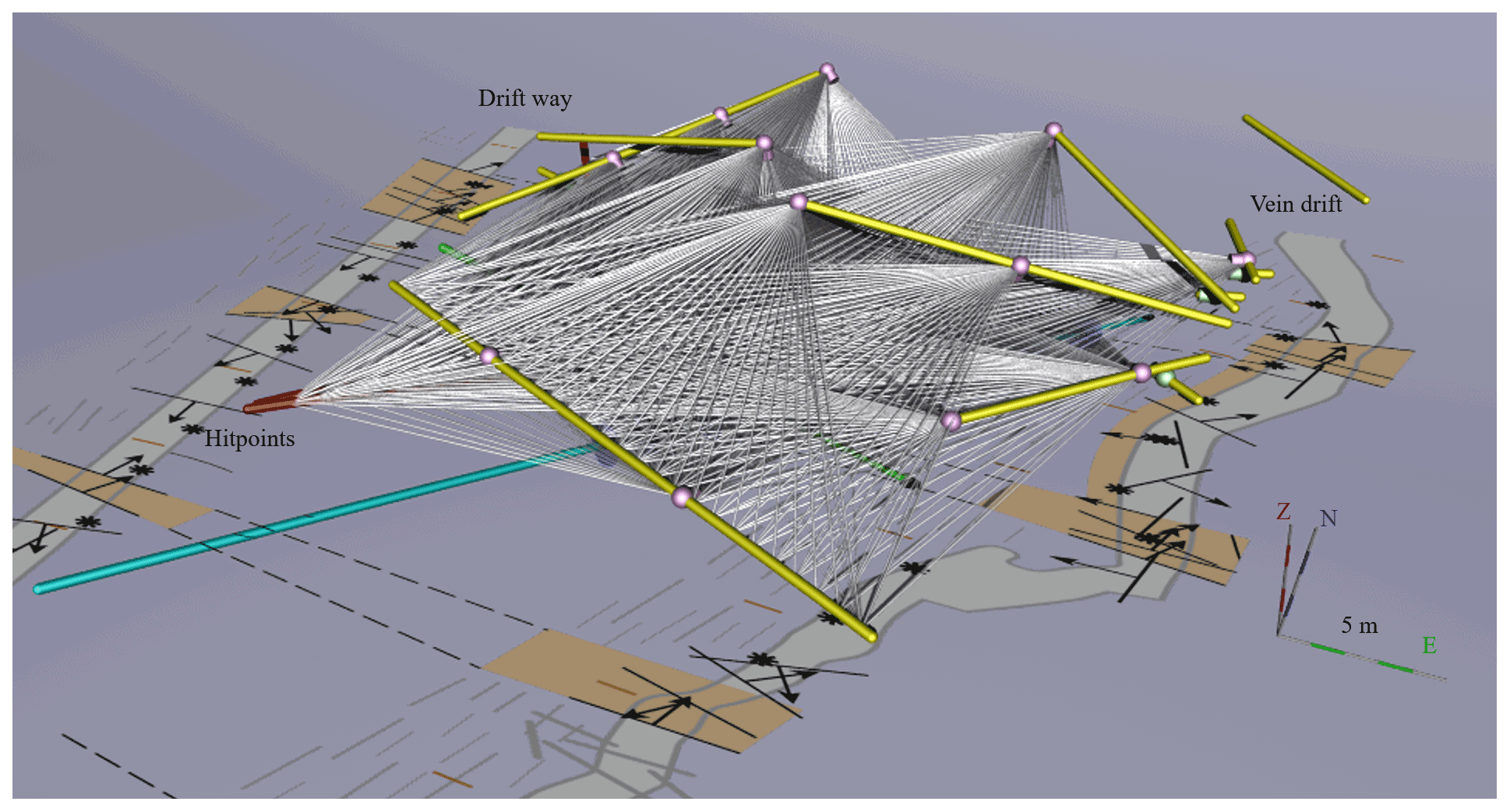
Figure 3Overview of active seismic measurements within the STIMTEC volume; ray paths show coverage achieved using UT measurements from boreholes to sensors. See Fig. S3 for different 3-D views. Hit points (black stars) along the galleries mark positions of repeated active hammer and centre punch measurements.
Sledgehammer hits also served as a simple reference signal to mark critical monitoring periods during all phases of the experiment: three hammer hits before the start and three to six hits at the end of each hydraulic pumping operation allowed us to calibrate timing of the seismic and hydraulic observation systems, made different groups on site (located in different galleries during the stimulation) aware of operations and helped to distinguish working noise from the target AE signals.
In addition to the active surveys along the tunnel walls, >300 ultrasonic transmission (UT) measurements were performed in the hydraulic monitoring, injection, validation and cable boreholes for velocity model estimation. The single ultrasonic transmitter (central frequency ∼ 15 kHz) is charged slowly and then discharged rapidly, producing a delta pulse. At each measurement point, a total of 1024 of these pulses were automatically stacked on each sensor channel to improve the signal-to-noise ratio (SNR). The resulting signal generally contains more high-frequency energy than common AE signals (>30 kHz, Fig. S1). UT measurements in the injection borehole, with sources placed every metre along most of its length, were performed for velocity measurements before and after the stimulation. The side-view ultrasonic transmitter was pneumatically coupled to the borehole wall in three different orientations before the stimulation and at one orientation after the stimulation. By using different orientations, the maximum amplitude of the source radiation pattern was directed towards the AE sensor locations near driftway, directly above the injection borehole and along vein drift, respectively. As the UT source signal was generally recorded throughout the STIMTEC rock volume, only one orientation was adopted subsequently. The vertical validation borehole was sounded before and after stimulation, while the remaining validation and cable boreholes were sounded once at the end of the validation phase or the final hydraulic testing phase of the experiment, respectively (Fig. 3).
2.7 Passive seismic monitoring
To monitor injection-induced fracture processes and associated small-scale brittle rock failure, we focused passive seismic monitoring on small-magnitude (), high-frequency (fc≥300 Hz) AE events with expected fracture sizes ranging from a few centimetres to the metre scale (Bohnhoff et al., 2010). Similar monitoring was previously successfully applied (see review by Manthei and Plenkers, 2018; Kwiatek et al., 2018; Villiger et al., 2020).
Passive seismic (continuous and triggered) data were recorded during all injection operations. Triggering levels were adjusted during hydraulic pumping operations and tuned for each stimulation interval to minimise false triggers that lead to a dead time in the triggered recording system. Noisy channels were switched off to facilitate monitoring of many partly overlapping AE events in real time on site and to identify larger events. AE events detected in trigger mode were automatically picked and located in near-real time on site to obtain a preliminary catalogue and control the experiment. Outside of stimulation campaigns, the continuous-mode system was operated between 29 June and 14 August 2018 (with some data gaps; see Table S1 in the Supplement) and 5 November to 4 December 2019 (no gaps) to measure post-stimulation processes and to characterise potential background seismicity. We recorded >72 TB of seismic data by the end of the field experiment.
3.1 Data processing
The different phases of the STIMTEC experiment were accompanied by varying in situ noise conditions that affected predominantly the high-sensitivity AE sensors. Passive seismic data often showed contamination with transient electronic noise and noise generated by the hydraulic pumps during stimulation. To address this problem, we applied filtering using the continuous wavelet transformation. We first identified the wavelet coefficients related to transient noise signals by comparing continuous seismic data with and without noises. By removing the identified wavelet coefficients from the recorded wavelet spectrum, the unperturbed AE signal could be retrieved efficiently. This was possible because the AE signal and noise overlapped only partially in frequency content (Fig. S2).
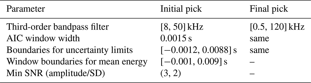
For post-processing of the triggered AE event data, we apply the automatic phase identification algorithm by Wollin et al. (2018), which is based on the two-step approach by Küperkoch et al. (2010) to first determine a preliminary arrival time, which is then refined by suppressing noise and using a wider causal bandpass filter. The waveforms are first filtered using a third-order Butterworth bandpass filter before a rolling higher-order-statistics kurtosis filter is applied to determine a preliminary onset time. Then, by systematically calculating suites of Akaike information criterion (AIC) functions on rolling and nested time windows of wavelet portions containing the phase onset, the variability of the global minima is used to estimate the final pick as well as an asymmetric pick uncertainty. Parameter settings are given in Table 4. The same procedure is applied for P and S arrivals. However, given the single-component data and the AE sensor's typical post-pulse oscillations, automatically picked S arrivals are considered uncertain in this study. We observed that the amount of automatically picked S arrivals is significantly larger than for a reference dataset of manually picked S arrivals. The reference dataset, comprising 300 events with 2286 manual P picks and 1021 S picks, was used to tune the automatic picking algorithm.
3.2 Velocity model
We used the active seismic UT measurements to derive a velocity model. UT data were manually inspected, and arrival times of the P and S waves, as well as the origin time of the UT source pulse, were identified. We distinguished between impulsive, high signal-to-noise ratio P-wave arrivals and more emergent, low signal-to-noise ratio P onsets. Given the known origin time and location of each UT measurement point, travel times to the seismic sensors were calculated assuming straight ray paths (Figs. 3 and S3). Uncertainties of the obtained velocities were assessed from repeated measurements from each point in the injection borehole.
The Freiberg gneiss displays a prominent subhorizontal foliation and was expected to show transverse isotropic elastic properties as seen from core measurements (Adero, 2020) typically showing high P-wave velocities parallel to the foliation and low P-wave velocities perpendicular to it. To describe the observed anisotropy of the obtained velocity values, we applied the exact phase velocity equations for transverse isotropy (Thomsen, 1986, Eqs. 10a–d):
where ε and γ describe the strength of anisotropy for P waves and for S waves, respectively, vP0 or vS0 are velocities along the symmetry axis, and θ is the phase angle. The parameter D* is defined as
with
The angular dependence of the velocity is given by the shape factor δ.
Using the full description is significantly more complex than the weak anisotropy approximation:
which was derived by Thomsen (1986) for weak-to-moderate strength of anisotropy (). This approximation is commonly applied and describes the actual transverse isotropy accurately along and perpendicular to the symmetry axis but not at intermediate angles.
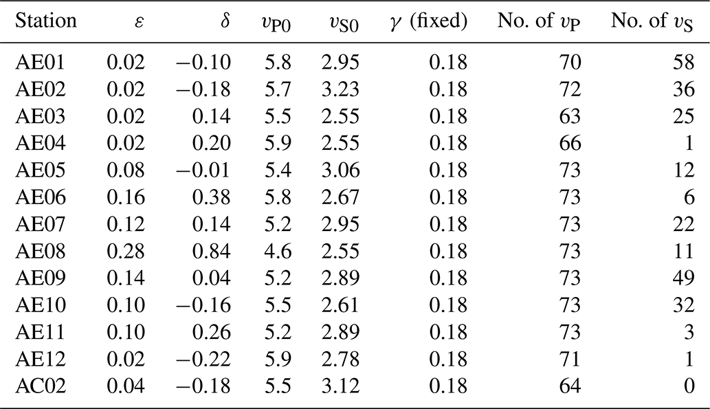
We determined Thomson's anisotropy parameters for P waves () for each seismic station assuming full transverse isotropy with a vertical symmetry axis. There was no angular asymmetry observed in the measured velocities that would indicate a tilt of the symmetry axis. We assume that the recorded wave velocities represent phase velocities rather than group velocities. We first calculated all wave velocities by systematically varying ε, δ in steps of 2 % and vP0 in 100 m s−1 steps. Then, the residual between computed and measured P-wave velocities were computed in a comprehensive grid search over the sampled parameter ranges. Due to the scarcity of S-wave observations in the UT data, the ratio of P- to S-wave velocities () along the vertical symmetry axis and the S-wave velocity anisotropy parameter γ were fixed to 1.77 and 18 %, respectively. These estimates were based on Wadati (1933) plots for near-vertical ray paths and sonic logs from a 70 m long, vertical borehole of the GFZ lab (Giese and Jaksch, 2016). This sonic log shows the average value at shallow and deep depths but a large deviation for intermediate depths. The value is slightly larger than the average value obtained from the sonic log in the (15∘-inclined from horizontal) injection borehole. Both logs exhibit large scatter (±0.15). To determine the set of best-fitting Thomsen parameters per station (Table 5), we compared the parameter ranges for the best 10 and 100 models. This velocity model was referred to as the best transverse isotropic velocity model per station. It was compared to an isotropic velocity model (vP=5600 m s−1, ) and a single transverse isotropic velocity model for all stations (vP0=5300 m s−1, ε=11.3 %, δ=0, ).
Table 5Thomsen parameters (ε, δ and γ) characterising elastic anisotropy of the rock mass derived from fitting all active seismic UT measurements per seismic station. The last two columns give the numbers of measurement points for vP and vS, from which the parameters were derived.
To clarify limits on the detection ranges as a function of distance, attenuation and anisotropy at the decametre scale, we investigate attenuation characteristics of the rock. Attenuation estimates of the elastic waves travelling in the fast anisotropy direction parallel to the foliation were obtained using hammer and centre punch hits.
We assume that the amplitude A of the wave decays with distance d from the active source according to
where A0 is the amplitude at the source, G is the gain factor of the recording sensor, and γ is the anelastic attenuation coefficient. This neglects the effect of scattering. By multiplying the measured (assumed S-wave) amplitude by the distance, taking the natural logarithm and dividing by the distance, we see that γ can be obtained. We fit the data of the logarithm of the normalised amplitudes of sensors with the same gain against the distance from the source, with a regression line, where the slope m is proportional to the attenuation coefficient of the medium.
For each of the 10 hammer hits at each hit point along the galleries, an 8 ms time window starting at the P arrival was chosen, from which the maximum amplitude value was extracted for each AE sensor. Then, the dominant frequency of the signal was determined for each AE sensor from the maximum amplitude in the frequency range containing 99 % of the energy of the signal. The average of the dominant frequency from all sensors fdom together with the slope of the regression line m and the average S-wave velocity vS90 in the horizontal direction were used to estimate the quality factor Q, according to
Similarly, attenuation estimates were obtained by comparing waveforms of centre punch hits recorded by accelerometers located in opposite galleries with one sensor next to the hit point. Spectral amplitude ratios were analysed to obtain an estimate of the quality factor.
3.3 Hypocentre locations and velocity model uncertainty
During post-processing, hypocentre locations were determined using the equal differential time (EDT) method by Zhou (1994) combined with a downhill simplex optimisation algorithm (Nelder and Mead, 1965) applying the developed transverse isotropic velocity model derived for each station. The EDT method has the advantage that the inversion of the hypocentre location is based on the relative arrival times of pairs of P- and S-wave arrivals at the same station or pairs of P arrivals at different stations. The origin time is not specifically inverted for but obtained as a byproduct. Gischig et al. (2018) demonstrated how the inversion for origin time, hypocentre location and station corrections are affected by anisotropy. Applying the weak anisotropy approximation, these authors calculated the velocity-dependent derivatives required for the inversion. We did not specifically account for anisotropy in the location procedure, because the non-linear EDT method can handle 3-D heterogeneous velocity models. Instead, we used the anisotropic velocities in the forward computation of the calculated travel-time grids, from which the EDT surfaces were determined. We tested the method by relocating the known UT measurement points using the manually identified P-arrival times with the derived velocity model per station.
To locate the AE events, we derived an initial hypocentre location based on P-wave arrivals only and a final location including only those S arrivals consistent with the initially derived hypocentre. To be included in the location procedure, the root-mean-squared (rms) residual for an S arrival needed to be less than 1.5 times the rms of the P arrivals for the initially derived hypocentre ensuring that inaccurately autopicked S arrivals were discarded. The rms is defined as
where ti are calculated and observed travel times for i stations and wi is the weight. Phase weighting for autopicked P arrivals was implemented, based on the SNR, with SNR ≥ 6 obtaining full weight, 6 > SNR ≥ 3 half weight and SNR < 3 of the full weight. S arrivals were weighted with of the full weight if included in the hypocentre estimation. We consider only events with a minimum of five phase arrivals and display those hypocentre locations with rms travel-time residuals below a selected limit of 2 ms. We also applied station residuals obtained as average P-wave travel-time residuals per station.
To assess the influence of the applied velocity model on the hypocentre locations, we compared the median rms travel-time residuals of all AE event hypocentres obtained using different velocity models as well as the location uncertainty of the relocated UT measurement points. By comparing the relocation error from the isotropic velocity model with the transverse isotropy model and the best transverse isotropic velocity model per station, we provide estimates for the location uncertainty associated with inaccurate velocity models.
4.1 Constraints on velocity models and location uncertainty
Using a transverse isotropic velocity model per station, we obtained more accurate locations (lower rms travel-time residuals, Table 6) and reduced the uncertainties determined from re-locating the known UT measurement points (using the manually identified arrival times and the derived vP and vS velocities, Fig. 4) compared to using an isotropic velocity model or a single transverse isotropic velocity model for all stations. The latter was determined from the averaged Thomsen parameters of all stations (Table 5). The network geometry influences the direction, while the velocity misfit determines the location uncertainty (length of the black bars in Fig. 4a). The best velocity model per station results in an average relocation error of 0.26±0.06 m for the active seismic UT measurement points in the range 22–31 m borehole depth in the injection borehole (Fig. 4b), along which the majority of AE events were observed, compared to 2.6±0.20 m for isotropic and 0.49±0.12 m for the single transverse isotropic velocity model. Relocation of the UT measurement points was based on using only P-arrival times. Adding the S-wave arrivals did not further reduce the location errors. This is likely because there are only few S picks (on average, three per measurement point for the injection borehole and five for the vertical validation borehole, compared to on average 12 and 13 P picks, respectively) identifiable in the UT data. Note that the S-wave velocity model is not well constrained, but the few S arrivals observed in the active UT dataset are consistent with the assumed S-anisotropy parameters (vS0,γ).
Table 6Comparison of root-mean-square residual and number of obtained event locations in the injection (IB) and vertical validation borehole (VVB) obtained using different velocity models. For location accuracy assessment, the average relocation error of the known UT measurement points outside of identified damage zones is provided, which represents an average of all values shown in Fig. 4b.
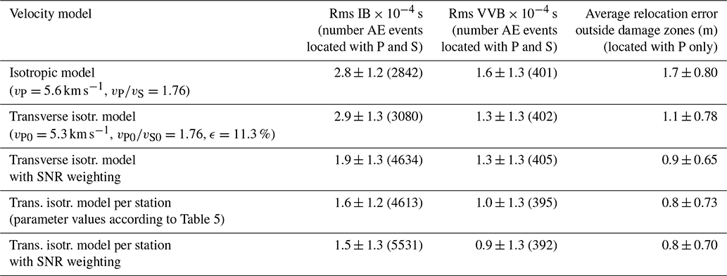
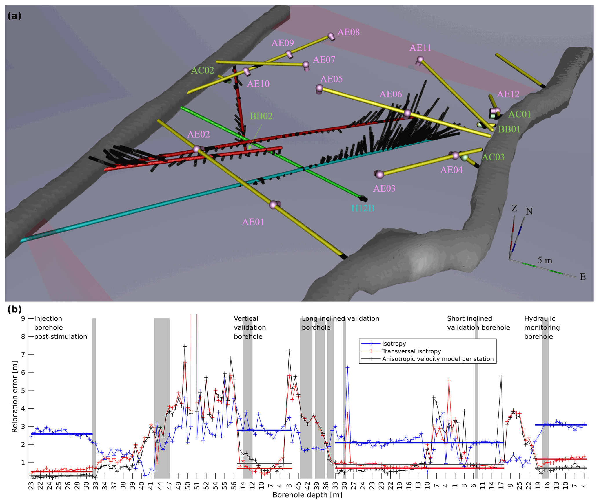
Figure 4(a) Overview of location uncertainty estimates (black lines) along the injection, vertical and horizontal validation boreholes as estimated from locating known UT measurement positions (see Fig. 3) with the derived best transverse isotropic velocity model per seismic sensor. Note that the location error becomes larger than 1 m, where the injection (cyan) and long inclined validation borehole (red) show higher numbers of fractures and more prominent ones (cf. Fig. 2). As shown in more detail in Fig. S4, the estimated location uncertainty is systematically directed upwards, likely a result of the station distribution. Labels refer to AE sensors (pink), accelerometers or broadband sensor (green, with the broadband sensor being moved to a new position during the experiment) and AE hydrophone (blue). Deformation zones (pink zones) that transverse the rock volume between the galleries are also shown. (b) Comparison of location error of known active UT measurement points in the injection, vertical and horizontal validation boreholes as well as the hydraulic monitoring borehole for different velocity models. Relocation errors in black are obtained using the best transverse isotropic velocity model per station, in red from the single transverse isotropic velocity model and in blue from the isotropic velocity model. Coloured horizontal lines represent average relocation errors for the given depth range. Note that the anisotropic velocity model per station minimises the location uncertainties over most depth ranges in all boreholes, except for the vertical validation borehole, where the single transverse isotropy model performs slightly better. The isotropic velocity model performs better at larger borehole depths (where no AE events were observed) and in the wider fracture zones of the injection and long validation boreholes (as indicated by the vertical grey bars, which correspond to the sections shown in Fig. 2).
The best transverse isotropic velocity model per station also provided the lowest relocation error on average along the injection borehole outside the damage zone (borehole depths < 40 m), where the resolution accuracy is decreased by 70 % for the isotropic model and 29 % for the single transverse isotropic model (Table 6), respectively. We note that the best velocity model per station is tuned to the injection borehole because its number of measurement points is largest. This effectively provided a 4 times higher weight for measurement points along the injection borehole (compared to double weight for the vertical validation borehole and single weight for all other boreholes). For relocating the known UT measurement points in the vertical validation borehole, relocations obtained using the single transverse isotropic model (average relocation error of 0.69 ± 0.53 m, Fig. 4b) are more accurate than for the best velocity model per station (average error 0.95 ± 0.46 m). For all other inclined boreholes, the best velocity model per station results in the lowest relocation uncertainties compared to the other velocity models (Fig. 4b). The isotropic velocity model performs best in relocating the known UT measurements in the wider deformation zones in the injection and long inclined validation borehole based on the relocation error, compared to the anisotropic velocity models. Within the deformation zones, all models show a systematic mislocation upwards above the injection borehole (Figs. 4a and S4), reflecting predominantly the seismic network geometry.
4.2 Structural heterogeneity, velocity and attenuation
We investigated the influence of the various geological structures in the rock volume on the seismic wave propagation and on the velocity model. The background anisotropy caused by the strong foliation of the host rock is overprinted by structural heterogeneity on site. We observed significant velocity reductions of 1 %–4 % per station over several UT measurement points (Fig. 8a) associated with a prominent fault, identified at 32.5 m in the injection well (Fig. 2). For most stations, this vP drop is larger than the velocity uncertainties obtained from three to six repeated measurements from in total 48 points, predominantly in the injection borehole. The standard deviations for these repeated velocity measurements at all stations range between 1 and 145 m s−1 with mean values of 35 m s−1.
We also see significant misfit between the velocities predicted by the anisotropic velocity model and the observed velocities for deformation zones at borehole depths >42 m in the injection borehole and >32 m in the long validation borehole (Fig. 4). At these depths, the logged structures and elevated fracture densities likely affect seismic wave propagation by strong attenuation and deviating ray paths. This suggests that the velocity models fitting the anisotropic reservoir rocks are inadequate for prominent faults and surrounding damage zones.
Close to the prominent fault at 32.5 m depth, we observe an amplitude reduction of the stacked UT signal by up to 50 % compared to the values of neighbouring measurement points. This value was determined as the difference between the actual value and the value expected for these depths from linear regression of three neighbouring amplitude measurements at shallower and deeper depths. Still, ambiguity prevails as other factors such as UT source coupling and resonances at the receivers can also affect the recorded amplitudes. In general, we do not observe a systematic velocity or amplitude reduction from UT measurements in the injection borehole after stimulation as compared to before. Attenuation estimates of the elastic waves travelling in the fast anisotropy direction parallel to the foliation obtained from hammer and centre punch hits result in QP∼50 near the galleries and QP∼150 in the centre of the rock mass.
We observed good SNR ratios for UT measurements in the records of the three accelerometers for distances ≤ 15–18 m. For both accelerometers located off vein drift, we observed clipping of active centre punch hits generated at 10–15 m distance with incidence angles around 90∘ to the accelerometer axis. This likely reflects resonances and/or coupling issues. UT measurements are not recorded beyond distance of 31 to 33 m by the AE sensors. The AE hydrophone recorded UT signals with good SNR for distances smaller than 17 m (cf. Boese et al., 2021a). This reduced recording range compared to the AE sensors is likely related to the impedance contrast of the water-filled borehole and the rock. For this reason, AE hydrophones need to be placed as close as possible to stimulated intervals or, alternatively, installed permanently by cementation, which reduced the impedance and increases the sensitivity.
4.3 Seismic monitoring and network sensitivity improvements
The hydraulic stimulation campaign started in the deepest part of the 63 m long injection borehole with an intended progression of stimulation from deep to shallow intervals (Fig. 1). No AE activity was observed during stimulation of the two deep intervals at 56.5 and 51.6 m borehole depths, closest to the highly fractured damage zone encountered at the bottom of the borehole. These intervals are located furthest from the seismic monitoring network (HF1 and HF2; Table 2). To test detection limits and the seismic monitoring equipment under the given noise conditions, we changed the intended order of the stimulated intervals, so that two shallow intervals (at borehole depth smaller than 30 m: HF3 and HF4) were stimulated next, followed by two intermediate-depth intervals (borehole depth between 30 and 45 m: HF5 and HF6) before returning to the deep intervals (borehole depth greater than 45 m: HF7 and HF8). We observed significant AE activity (several thousand events, Table 2, Figs. 5 and 6a) for the shallow stimulation intervals (22.4, 24.6 and 28.1 m) and high breakdown pressures (11–13 MPa). Seismic activity was not identified before the start of the stimulation and stopped shortly after shut-in. Few AE events were recorded during injection into intermediate-depth intervals (33.9, 37.6 and 40.6 m depths, Table 2). These events occurred diffusely throughout the pumping sequence (Fig. 6b). For the interval at 33.9 m the second lowest breakdown pressure (6.4 MPa) of all tests was observed, whereas the adjacent interval at 37.6 m exhibited the highest observed value (15.8 MPa), pointing towards significant spatial complexity. The breakdown pressure of interval 40.6 m (9.4 MPa) is comparable to those in the deep intervals at 49.7, 51.6, 55.7, 56.5 m, which show intermediate-to-low values (5.8–9.4 MPa, Table 2) and no AE events, neither during the stimulation nor during subsequent hydraulic testing phases of the experiment.
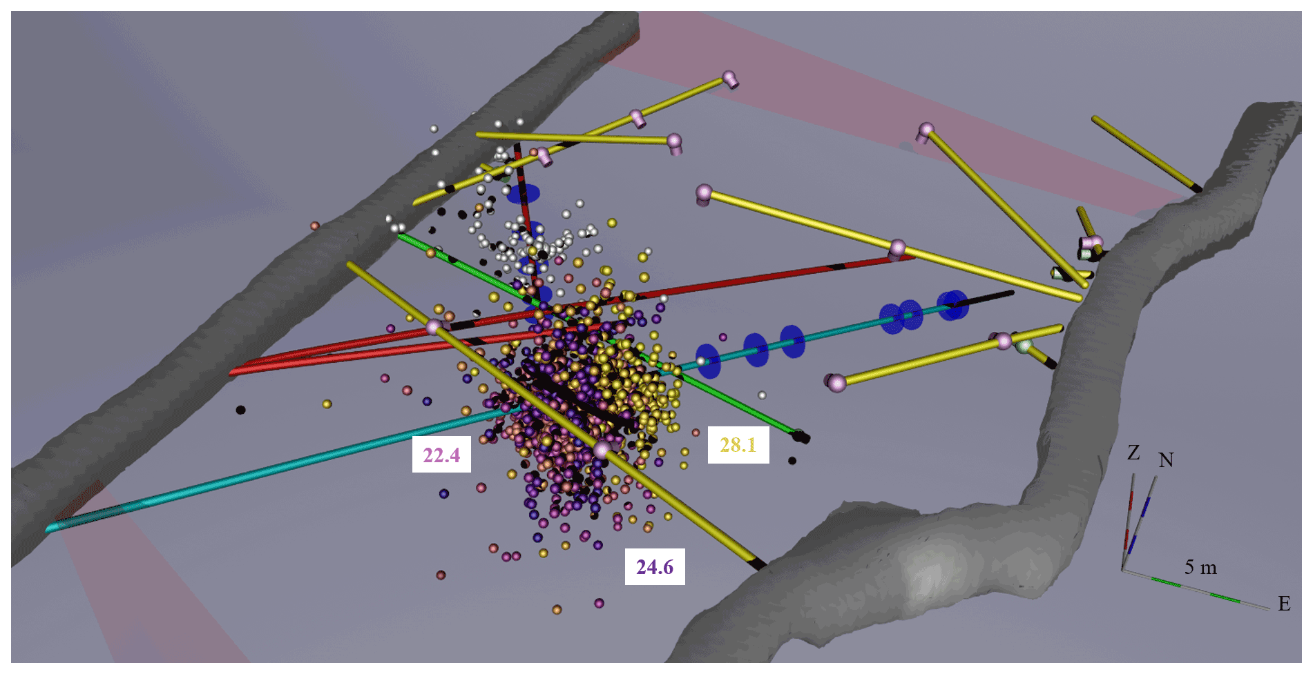
Figure 5AE locations obtained for stimulations in the injection borehole (coloured dots according to stimulated interval as marked) and the vertical validation borehole (white dots). See Fig. S5 for different 3-D views. Note that the intermediate-depth and deep stimulated intervals in the injection borehole produced little to no AE activity.
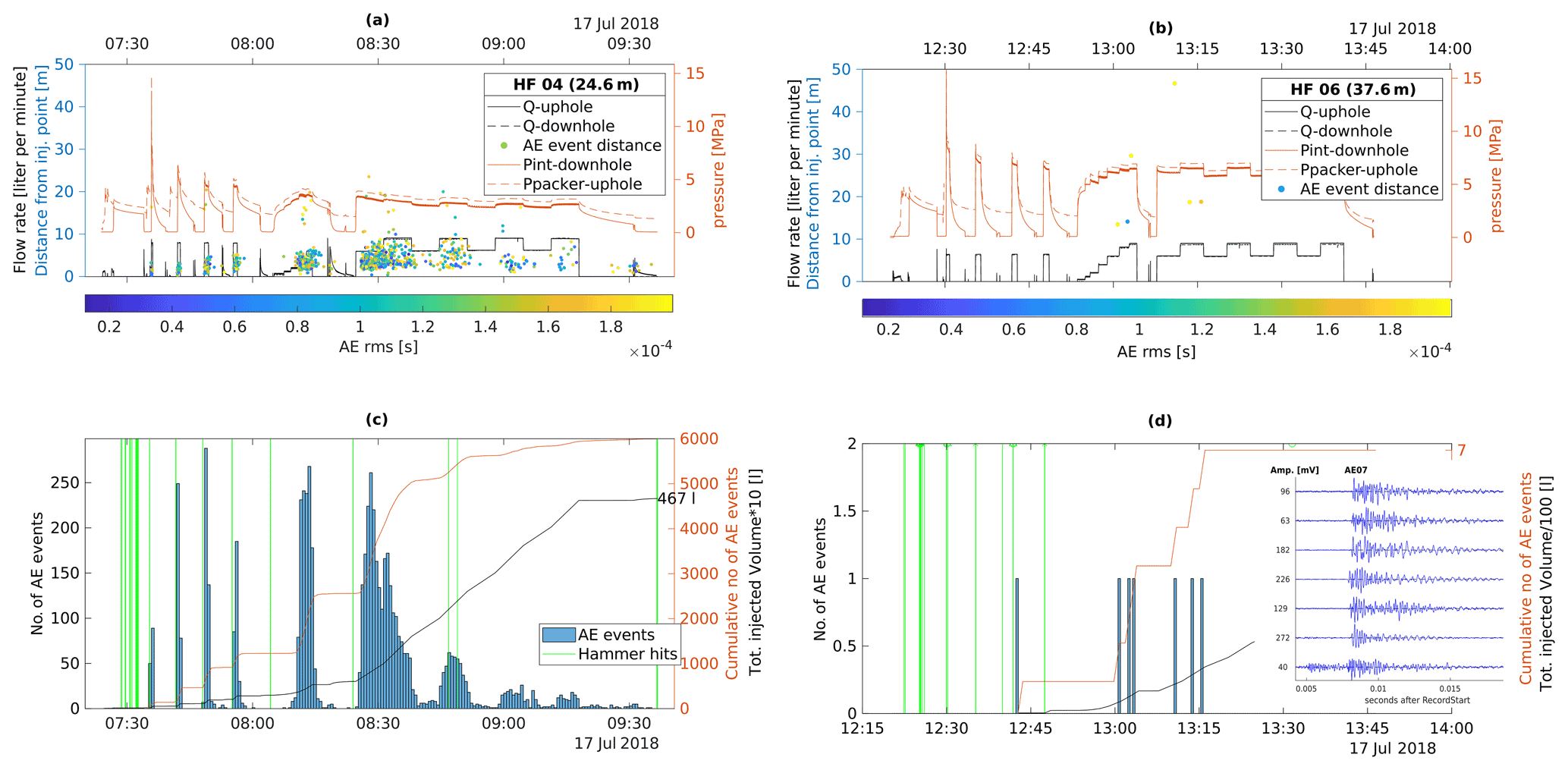
Figure 6Stimulation sequence consisting of a frac, three refracs, step-rate pump test and periodic pumping test for the intervals at 24.6 and 37.6 m borehole depths in the injection borehole. Panels (a) and (b) show flow rate (black) and pressure records (orange) measured in the intact intervals downhole and at the wellhead uphole as well as the AE activity plotted with distance from the centre of the injection interval (coloured dots). Panels (c) and (d) show an AE event histogram (blue), the cumulative number (orange) of located AE events and the cumulative injected volume (black). Active hammer hits (green lines) were used as marker signals throughout the injection sequence. An example of all the AE events observed during stimulation of interval 37.6 m as recorded by sensor AE07 is shown as an inset.
For stimulations of the seismically active intervals in the injection borehole (HF3, HF4, HF10; Table 2) and in the vertical validation borehole (HF12-15; Table 3, Fig. 5), we observed a general correlation between AE activity, fluid-injection cycles and volumes, when the injection pressure exceeded the fracture opening pressure. A small number of AE events occurred during the frac and refrac sequences (5–70 AEs per sequence), whereas significantly more events were observed during subsequent step-rate tests (75–180 AEs above jacking pressure) and during periodic pumping tests (30–240 AEs per cycle, Fig. 6). We observed a progressive growth of the seismic clusters which extend about 5 m radially from the injection interval (Figs. 5 and 6). The subhorizontal foliation does not seem to noticeably influence event propagation and seismic cloud growth. Note that the seismic clusters from the injection and vertical validation borehole are spatially distinct (see also Fig. S5).
The highly variable seismic response to stimulation prompted us to relocate two of the 16 seismic monitoring sensors (Fig. 1) to test if the absence of AE activity results from limitations in network sensitivity or site characteristics. We placed one AE hydrophone at the bottom of the hydraulic monitoring borehole to verify AE detection levels for intermediate-depth and deep stimulated intervals in the injection borehole. The AE hydrophone recorded few AE events during further hydraulic testing and accidental re-stimulation of the intervals 37.6 and 40.6 m (at 6–8 m hydrophone-interval distance), respectively, but no activity was observed for intervals 49.7 and 56.5 m (at 10 and 17 m distance), confirming previous observations of no AE activity in the deep stimulation intervals and recording ranges for AE events of ∼ 30 m for AE sensors at the STIMTEC site. The borehole broadband sensor was moved to the bottom of the vertical validation borehole for the last phase of the experiment, so that it located at a comparable absolute depth as the deepest stimulated intervals in the injection borehole. This was considered beneficial because of indications that seismic wave attenuation perpendicular to the foliation may be larger than parallel to the foliation (Adero, 2020). Overall, the broadband sensor recorded characteristic signals during hydraulic stimulations of all intervals in the injection borehole on 16–18 July 2018 (Figs. 7 and S7) that appear to respond to the flow rate rather than the injection pressure (Table S2 and Fig. S6). These signals were not recorded by the only other nearby broadband sensor, FBE (SX Net, distance 438 m SE of STIMTEC site; University of Leipzig, 2001). The observed signals vary in amplitude and period and are best observed on bandpass filtered (0.001–1 Hz) daily seismograms on the second horizontal component of the ASIR sensor, likely aligned parallel to vein drift (perpendicular to the borehole). There are also spike signals observed that may indicate rapid tilting and recalibration of the sensor (see also Fig. S7), based on shake table calibration after the experiment. They occur during operations at the site and their interpretation currently remains unclear.
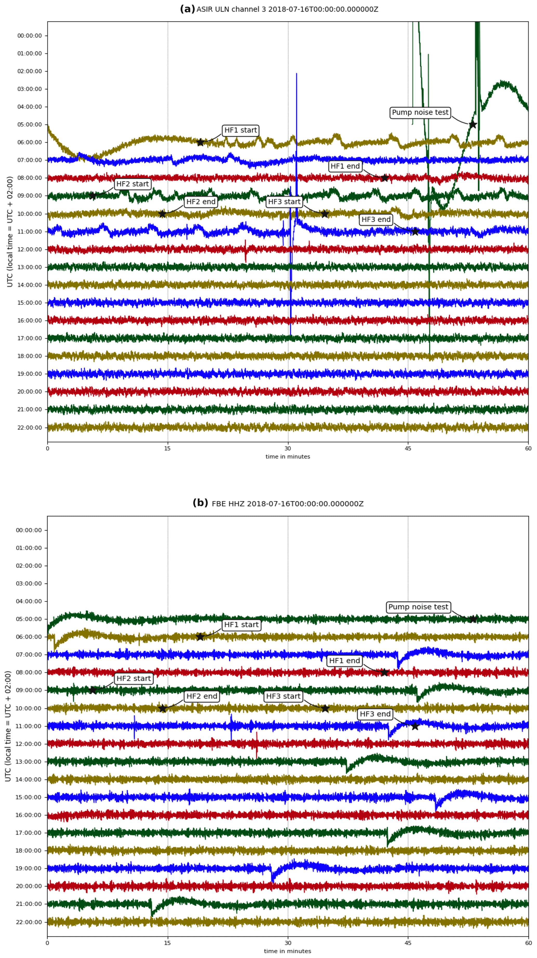
Figure 7Daily records of the horizontal channel of the ASIR and vertical channel FBE broadband sensor located at Reiche Zeche mine for the first day of stimulation on 16 July 2018. The distance between both sensors is approximately 440 m. Hydrofrac start and end times are marked (by stars) as listed in Table 2. Note that long period swings in the records result from bandpass filtering (0.001–1 Hz) in combination with data gaps as seen for the beginning of the records for the ASIR sensor and throughout the day for FBE. Some local quarry blasts are seen on both sensors, whereas stimulation related signals are only visible on the ASIR broadband sensor deployed at the STIMTEC site. Note that the two largest drops seen for the ASIR sensor are likely associated with sensor self-centring as determined on a shake table at GFZ lab after the experiment. See Fig. S7 for the other stimulation intervals during the following 2 d of stimulation.
5.1 Seismic monitoring network
Using a seismic monitoring system consisting of AE hydrophones, AE sensors, accelerometers and broadband sensors bears several advantages. The AE hydrophone can be attached on hydraulic tubing and therefore installed in combination with hydraulic equipment. This places it much closer to the stimulated intervals and as a consequence, AE hydrophones can enlarge the 3-D density of sensors and their coverage in the volume of interest, thus improving location accuracy and focal mechanism determination. This comes at the cost of reduced recording ranges and frequency bandwidth compared to common AE sensors (and reduced S-wave sensitivity; cf. Boese et al., 2021a).
All dedicated seismic monitoring boreholes were located above the stimulated volume to ensure that water entering into the boreholes can drain during the experiment. This posed the general problem of increased location uncertainty in the vertical direction. However, with this setup we achieved the desired monitoring quality without needing an extra monitoring borehole placed close to the stimulation borehole. During the EGS Collab and GTS experiments, the intersection of growing fractures with nearby monitoring boreholes caused immediate pressure release, inhibiting or deflecting fracture growth (Schoenball et al., 2020; Fu et al., 2021). This illustrates the problem that monitoring boreholes may impinge on the stimulation. Therefore, high-sensitivity AE sensors placed at some distance (20–30 m, considering the site characteristics of the STIMTEC experiment) to the stimulated intervals combined with AE hydrophones placed close to the stimulated interval in the stimulation borehole (above the double packer) likely offer the best solution for high-resolution seismic monitoring during hydraulic stimulation in URLs. However, preservation of the high-frequency content of seismic waves is site dependent and a prerequisite for the analysis of source properties of AE events with expected fracture sizes at the decimetre scale (e.g. Kwiatek et al., 2011). Empirical results of Plenkers et al. (2010) provide upper bounds for detection limits of AE events in low-attenuating hard rocks at ∼ 3 km depth. In the more general case, we refer to the modelling of detection limits for high-frequency energy of microseismic events by Kwiatek and Ben-Zion (2016).
Adapting the stimulation on site by changing the stimulation order in the injection borehole allowed for testing the sensitivity of the monitoring system and site conditions but also resulted in the stimulation of the most seismically active intervals (HF3, HF4, HF10; Table 2, Fig. 5) on three subsequent days. This adaption was possible because of the near-real-time processing and visualisation of AE events on site. It allowed us to separate the temporal distribution of the AE events in the spatially overlapping seismicity clouds (Fig. 5).
5.2 Seismic response to stimulation
We observed significantly different seismic and hydraulic responses of intervals separated by only a few metres in heterogeneous, metamorphic rock (Figs. 5 and 6). This generally agrees with observations from the AHRL, GTS and EGS Collab experiments, which also highlighted the influence of the rock type, the pre-existing fracture zones and stress heterogeneity on seismic responses to hydraulic stimulation. Although it is not yet clear what causes the large variability in deformation behaviour at the STIMTEC site, we verified that it is not primarily the result of detection capabilities of the seismic monitoring network along the injection borehole. We posit that deformation in response to stimulation in the deepest part of the injection borehole is predominantly aseismic (in the frequency band 1–40 kHz, corresponding to length scales in the centimetre-to-decimetre range). This observation is based on the absence of AE events and a strong long-period signal recorded by the broadband sensor. We suspect the observed variability in seismic response to stimulation is likely caused by rock-mass heterogeneity and the response of pre-existing fractures. In addition, injection boreholes not aligned with one of the principal stress orientations show complex fracture initiation (Rummel, 1987; Haimson and Cornet, 2003), likely controlled by small-scale material heterogeneities at the borehole wall, as also observed in lab experiments (Masuda et al., 1993). Reorientation of fractures with growth away from the injection interval has been observed previously in boreholes misoriented with respect to the principal stress axes, for example, by mine-back in soft volcanic rock (Warren and Smith, 1985) and by AE event cluster orientations in crystalline rocks (Gischig et al., 2018; Schoenball et al., 2020) and salt rock (Manthei et al., 2001). Re-orientation of AE event clouds has not yet been identified during the STIMTEC experiment. We note, however, that unexpected (based on stress modelling), strong, local variations of the stress magnitudes in the experimental volume were observed from stress measurements in the injection and vertical validation boreholes (Adero, 2020). The variability of shut-in pressures (with the largest deviations from the average values observed in the adjacent stimulation intervals at 33.9 and 37.6 m depths in the injection borehole) and orientations of induced fractures suggest overall small-scale stress heterogeneity at the STIMTEC site (Adero, 2020).
The observed low-frequency broadband recordings are similar to the broadband records observed by Zang et al. (2017, their Fig. 11) at the AHRL. In particular, we obtained strong signals from stimulations that did not yield high-frequency AE events. We also observed transient low-frequency signals recorded shortly before the start of the stimulation (Fig. S6). In particular, they correlate with the flow record associated with the installation of the hydraulic equipment, and we assume that these signals result from packer setting and flushing, causing transient low-frequency amplitude signals. These observations require further investigation to determine what causes the low-frequency broadband signals. Nevertheless, our observations suggest that borehole sensors sensitive in the frequency range 0.01–100 Hz positioned at distances of 19.6–26.6 m are adequate to monitor low-frequency deformation signals associated with hydraulic stimulations.
5.3 The role of anisotropy and heterogeneity for mine- and lab-scale experiments
Laboratory and active seismic measurements from the STIMTEC experiment show moderate to strong elastic wave anisotropy controlled by the pronounced foliation of the gneiss. We compare the here-obtained Thomsen parameters to those values determined in a range of laboratory tests on cylindrical Freiberger gneiss samples at different confining pressures (≤30 MPa) and orientations at room temperature (Adero, 2020). P-wave velocity measurements on samples in the laboratory exhibit similar mean values and ranges for wave propagation in different orientations with respect to the foliation as observed in field measurements. In laboratory tests, P-wave velocities for ray paths parallel to the foliation are slightly larger, about 20 % higher compared to the direction normal to the foliation (Fig. 8). This is irrespective of the significant differences in frequency bands of UT sources in the laboratory (500 to 800 kHz) and in the mine (5 to 60 kHz). Uncertainties of the obtained velocities in the field range between 1 and 145 m s−1 with mean values of 35 m s−1 for all stations, corresponding to 0.1 %–4.2 %.
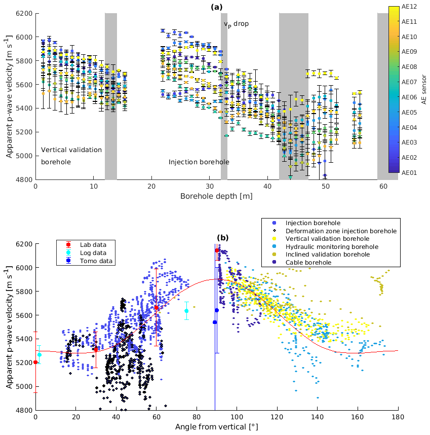
Figure 8Apparent velocities obtained from the source–receiver distance divided by the travel time from UT measurements used for calibration of the transverse isotropic P-wave velocity model. (a) Average apparent velocities with uncertainty estimate (<145 m s−1) against measurement depth in the borehole and (b) velocity against the angle relative to the vertical symmetry axis. The red line shows the theoretical P-wave velocities with incidence angle as determined using the Thomsen parameters derived from the laboratory measurements on Freiberg gneiss samples (α=5300 m s−1, δ=0.12, ). Measurement ranges obtained from sonic logs (cyan) from the vertical borehole in the GFZ lab and from the 15∘-inclined STIMTEC injection borehole are shown, as well as from P-wave tomography parallel to the foliation direction in the GFZ lab (blue). Velocity estimates obtained in the deformation zone in the injection borehole as shown in Fig. 2 are marked by grey bars in panel (a) and black points in panel (b). See also Fig. S8 for the other inclined boreholes.
At the STIMTEC site, P-wave velocities for ray paths parallel to the foliation are on average 12 % higher than perpendicular to the foliation for UT data. A large number of active UT field measurements were needed to cover the range of incidence angles necessary to determine the degree of P-wave velocity anisotropy and the symmetry axis of the metamorphic rock (Figs. 3 and S8). Near-vertical ray paths (parallel to and at acute angles to the symmetry axis) were difficult to obtain due to geometrical constraints limiting sensor positioning. In general, we observed a trade-off between the obtained P-wave velocity along the symmetry axis vP0 and the P-wave anisotropy parameter ε for the UT data (Fig. S9). This is likely an effect of missing constraints near the symmetry axis because of few near-vertical ray paths for the majority of stations. The two stations located furthest above the injection borehole with the highest number of near-vertical incidence angles display intermediate ε values of 8 %–12 % and vP0 = 5200–5400 m s−1. The average velocities of vP0=5275 m s−1 and vS0=2980 m s−1 from a sonic log for comparable depths in the vertical borehole of the nearby GFZ lab is consistent with the obtained velocity models. The average horizontal velocities of vP90=5650 m s−1 and vS90=3260 m s−1 from sonic logs in the injection borehole at the STIMTEC site are lower than the average velocities obtained for near-horizontal wave propagation from the UT data (Fig. 8). These sonic log velocities are more consistent with P-wave velocities derived for foliation-parallel wave propagation at the GFZ lab. We interpret the lower values to reflect the effect of dispersion, given the frequency content of the measurement (4–30 kHz for sonic log, 0.15–3 kHz for tomography at the GFZ lab versus 5–60 kHz for active UT at the STIMTEC site).
Anisotropy complicates the analysis of all measurements in the STIMTEC test volume, especially regarding velocity model calibration and AE event location. In retrospect, we estimate that approximately one-third of all active UT measurements in combination with the lab measurements, sonic logging and other available information (Krauß et al., 2014) would have been sufficient to characterise the single transverse isotropic velocity model, which captures the general features of the background anisotropy on site. This implies that the effect of dispersion is insignificant. However, to resolve the best-possible velocity model for each station and to obtain high-accuracy AE event locations required a transverse isotropic velocity model per station, derived from a large amount of active in situ velocity measurements covering a range of incidence angles. The best velocity model per station allowed for a significant location improvement of AE events from the injection and vertical validation borehole as shown by comparing the rms travel-time residuals for different velocity models as well as the relocation error of known active UT measurement points along the boreholes (Table 6). Neglecting anisotropy would lead to significant and systematic location bias by up to 2.6 m (Fig. 4b). The average P-wave anisotropy for the STIMTEC site is larger than observed for the granite and granodiorite host rocks at the GTS (∼ 7 %) and AHRL but comparable to the phyllites at SURF (Gao et al., 2020). Gischig et al. (2018) showed that at the GTS similar but slightly more scattered AE event clouds could be obtained using the joint hypocentre determination method with an isotropic velocity model and station corrections for AE event locations compared to using the anisotropic velocity model. Their approach is based on the weak anisotropy approximation, but it suggests that the effect of anisotropy can be mitigated this way. However, 32 seismic stations were installed at the GTS and structural heterogeneity is not as pronounced there as at the STIMTEC site, because the shear zones are similar in orientation compared to the foliation causing anisotropy in the rock volume. Our work demonstrates that high-resolution AE event locations (average rms of 0.00015 s) can be obtained in heterogeneous rocks with pronounced anisotropy, if an accurate velocity model can be derived. This requires numerous UT calibration measurements from various angles, which is achievable for URL experiments, some computational effort to derive the velocity model and a smart event location procedure. This demonstrates that hydraulic stimulation in complex rock such as anisotropic and heterogeneous metamorphic gneiss is possible and can be monitored (with additional effort), so future in situ experiments do not need to consider homogeneous rocks only.
Lab experiments also documented a strong influence of the foliation on the mechanical strength and therefore on fracture propagation and length (cf. Adero, 2020; Vervoort et al., 2014). The shallow depth of the STIMTEC site results in low absolute stress magnitudes (1–6 MPa) and lower differential stress conditions compared to URL sites elsewhere. To limit the effect of the foliation on the stimulation, the injection borehole was drilled at a 15∘ angle to the foliation. Despite the low absolute stress magnitudes, neither impression packer marks nor AE cluster orientations indicated that the foliation determined fracture propagation in the injection borehole. This was also found at SURF, where hydrofractures did not follow the strong foliation but the inclined maximum principal stress over tens of metres in the injection borehole (Oldenburg et al., 2016).
We observed significant velocity reductions (1 %–4 %) associated with prominent pre-existing structures, in particular in the deformation zones crossing the injection and long inclined validation boreholes (Fig. 8). In general, we do not observe a systematic velocity or amplitude reduction from UT measurements in the injection borehole after stimulation as compared to before. We conclude that only prominent pre-existing structures identified in logs have a significant effect (velocity drop larger than the average measurement uncertainty) on velocity and attenuation. Whether transient fluid pressure variations during the stimulation have a measurable effect on velocity (Doetsch et al., 2018) and/or attenuation at the STIMTEC site remains the subject of further investigations, which will be attempted using relative travel times from centre punch measurements as opposed to absolute travel times from UT measurements. P-wave attenuation factors determined here for the fast anisotropy direction are generally consistent with the values obtained for the GFZ lab (Krauß et al., 2014). Laboratory measurements revealed that attenuation perpendicular to the foliation is stronger than parallel to the foliation (Adero, 2020), but this has not yet been investigated from the obtained field data.
5.4 Implications for monitoring field-scale hydraulic stimulation experiments
In field-scale projects, sensor placement is significantly more limited and constrained than in mine-scale settings, where due to the 3-D placement of sensors in close vicinity of the injection a close to ideal situation for monitoring of a hydraulic stimulation experiment is achieved (similar to the laboratory scale). By avoiding permanent installations and temporarily removing seismic sensors, we could use the existing boreholes for different purposes throughout the STIMTEC experiment (e.g. for hydraulic monitoring, for passive seismic monitoring using different sensors, for stress measurements, repeating measurements to verify impression packer marks and for repeated active seismic measurements). Accessible boreholes provided us with more flexibility, especially as more boreholes became available during the course of the experiment. Adapting the monitoring (by implementing, testing and assessing a new AE hydrophone and a broadband borehole sensor) and modifying the order of stimulations proved successful to achieve the monitoring goals of STIMTEC. During a recent geothermal stimulation in Finland, adapting the stimulation procedure in response to high-quality real-time monitoring observations was critical for controlling fluid-induced seismicity (Kwiatek et al., 2019). Maintaining flexibility during experiments at the mine and field scale, which have less controlled conditions as compared to lab experiments, is a key element to address surprises and unexpected challenges, which seem inevitable given the higher degree of reservoir complexity observed at these scales. Flexibility requires good on-site communication between the various groups involved in the experiment, time and budget to allow for changes, as well as practical and integrated approaches to manage, exchange, visualise and interpret large 3-D datasets of different formats during the experiment.
Another observation of fundamental importance was that approximately half of the stimulated intervals were not accompanied by any AE activity, despite appropriate monitoring in place. Villiger et al. (2020) estimated the amount of aseismic deformation during hydroshear experiments at the GTS and compared this to the amount of seismic deformation, showing that aseismic deformation was dominant for both brittle and brittle–ductile structures. This estimation was based on the total moment, calculated from borehole dislocations of mapped fractures, compared to cumulative seismic moment of AE events and observed cloud extents. Guglielmi et al. (2015), De Barros et al. (2019) and Cornet (2016, and references therein) also showed that deformation is mainly aseismic during stimulations in softer rocks (shales, limestone) at the intermediate scale and sedimentary rocks at the field scale. To simultaneously capture fast and slow deformation processes, which are currently often categorised as either seismic or aseismic due to the limitations of current monitoring systems, requires better high-sensitivity instrumentation with a wider bandwidth. Alternatively, the combination of sensors with different sensitivity and frequency ranges (e.g. AE sensors, broadband, tilt, fibre-optic-based strain sensors) is necessary but requires time synchronisation and amplitude calibration, which can pose sophisticated technical problems (cf. Zang et al., 2017). To address these, marker signals and regular active seismic measurements proved valuable during the STIMTEC experiment. The mine scale has the advantage that new tools and/or different configurations (numerous sensor arrays) can be more easily tested, and maybe regular high-resolution laser-scan tunnel mapping (Grehl et al., 2015) can be applied as an equivalent tool to Interferometric Synthetic Aperture Radar (InSAR), which was successful in monitoring larger-scale slow deformation processes at the reservoir scale.
Mesoscale experiments currently provide the most-detailed in situ information to further understanding of hydromechanical processes associated with hydraulic stimulation and allow for validation of inferred results. In the here-presented STIMTEC experiment, conducted in the Reiche Zeche mine URL at 130 m depth, we used a high-resolution seismic monitoring network comprising 12 in situ AE sensors (for high-sensitivity monitoring of induced AE activity and the recording of active source signals), three accelerometers (for sensor cross-calibration purposes), one broadband sensor (to extend monitoring to the low-frequency range) and an AE hydrophone (to improve the network sensitivity in the deeper rock volume of the experiment). We relocated two monitoring stations and tested new sensors during the course of the experiment to optimise passive and active seismic monitoring. In contrast to other similar experiments, we stimulated strongly foliated rock with pronounced anisotropy during STIMTEC. We acquired a large quantity of active UT measurements for characterising the anisotropy and heterogeneity of the host rock. We monitored in near-real-time small-scale rock failure and friction processes associated with hydraulic stimulation and tracked the spatiotemporal distribution of AE events.
The key observations from the experiment are as follows: (1) we demonstrated that high-frequency (up to 100 kHz) seismic monitoring in complex rock volumes with pronounced anisotropy is possible, if measures are taken to accurately quantify the 3-D anisotropic velocity structure. (2) We applied Thomsen's exact phase velocity equations to deduce a transverse isotropic velocity model per station that accurately locates known active ultrasonic measurement points in the stimulated boreholes. Estimates of the uncertainties related to simplifications of the velocity structure and neglecting anisotropy significantly affect resolution and range between 0.5 and 2.6 m in our experiment. (3) We obtained average Thomsen parameters (P-wave anisotropy of 12 %) in agreement with those derived from laboratory and sonic logging data. (4) We observed that rock-mass heterogeneity as seen in high-fracture density zones overprints the anisotropy of the host rock and has a significant influence on velocity and attenuation. (5) We observed seismic responses to hydraulic stimulation in 10 intervals in the injection borehole, performed with similar injection protocols, ranged from abundant AE activity to no AE activity and are unrelated to monitoring limitations. We attribute the observed variability in deformation to the small-scale rock-mass and stress field heterogeneity observed in the injection borehole.
Our observations indicate that stimulation of strongly foliated and fractured rock mass, such as the Freiberg gneiss, results in activation of a complex fracture network. We infer that most of the induced deformation of the reservoir remains aseismic given the high number of stimulated intervals with little or without AE activity and the observed low-frequency signals recorded by the borehole broadband sensor. Aseismic deformation may be related to injection into open pre-existing fractures in the injection interval; yet, borehole logs do not systematically show pre-existing fractures present in “quiet” stimulated borehole intervals.
All active UT transmission data used in this study, sensor coordinates, measurement recording times and positions, as well as manually identified phase arrivals are available from the GFZ data server (https://doi.org/10.5880/GFZ.4.2.2021.002, Boese et al., 2021b).
The supplement related to this article is available online at: https://doi.org/10.5194/se-13-323-2022-supplement.
GD conceptualised the experiment and acquired funding for it; GD, GK and KP planned the experiment and its instrumentation; CMB, TF, KP, FB and CJ conducted fieldwork; JS and FB helped CMB with data curation. CB administered the project, formally analysed the seismic data and led the investigations. CMB wrote the manuscript with feedback and reviews by GD, GK and KP.
The authors (except Thomas Fischer, Katrin Plenkers and Felix Blümle) state that they are currently employed at the same institution as the journal's chief executive editor Charlotte Krawczyk.
Publisher’s note: Copernicus Publications remains neutral with regard to jurisdictional claims in published maps and institutional affiliations.
We thank LfLUG for providing fault surface data created on a small scale, a mine layout of the Reiche Zeche mine complex and surrounding mines and a digital elevation model. Staff from GMuG, Bad Nauheim, Mesy SolExperts, Bochum, and LIAG, Hannover, are thanked for their field measurement contributions to this project. Support by Frank Reuter and his team of miners at Reiche Zeche is gratefully acknowledged. Discussions with Joerg Renner and Marco Bohnhoff substantially improved the manuscript. We thank Chet Hopp and an anonymous reviewer for their detailed reviews.
This research has been supported by the Bundesministerium für Bildung und Forschung (grant no. 03G0874C).
The article processing charges for this open-access publication were covered by the Helmholtz Centre Potsdam – GFZ German Research Centre for Geosciences.
This paper was edited by Ulrike Werban and reviewed by Chet Hopp and one anonymous referee.
Adero, B.: Experimental investigations of mechanical anisotropy of Freiberg gneiss: implications for hydraulic stimulation, PhD thesis, Ruhr-Universität Bochum, https://doi.org/10.13154/294-7755, 2020.
Amann, F., Gischig, V., Evans, K., Doetsch, J., Jalali, R., Valley, B., Krietsch, H., Dutler, N., Villiger, L., Brixel, B., Klepikova, M., Kittilä, A., Madonna, C., Wiemer, S., Saar, M. O., Loew, S., Driesner, T., Maurer, H., and Giardini, D.: The seismo-hydromechanical behavior during deep geothermal reservoir stimulations: open questions tackled in a decameter-scale in situ stimulation experiment, Solid Earth, 9, 115–137, https://doi.org/10.5194/se-9-115-2018, 2018.
Bayer, M.: Die Himmelfahrt Fundgrube: ein Führer durch das Lehr- und Besucherbergwerk der TU Bergakademie Freiberg, TU Bergakademie, Verlag druckspecht, 1999.
Boese, C., Kwiatek, G., Fischer, T., Renner, J., and Dresen, G.: AE-type hydrophone performance during the STIMTEC and STIMTEC-X hydraulic stimulation campaigns at Reiche Zeche Mine, Germany, in: 55th US Rock Mechanics/Geomechanics Symposium, Houston, Texas, USA, 20–23 June, American Rock Mechanics Association, ARMA-2021-1724, https://onepetro.org/ARMAUSRMS/proceedings-pdf/ARMA21/All-ARMA21/ARMA-2021-1724/2482144/arma-2021-1724.pdf (last access: January 2022), 2021a.
Boese, C. M., Kwiatek, G., Fischer, T., Plenkers, K., Starke, J., Blümle, F., Dresen, G., and Janssen, C.: Ultrasonic transmission measurements from six boreholes from the STIMTEC experiment, Reiche Zeche Mine, Freiberg (Saxony, Germany), GFZ Data Services [data set], https://doi.org/10.5880/GFZ.4.2.2021.002, 2021b.
Bohnhoff, M., Dresen, G., Ellsworth, W., and Ito, H.: Passive Seismic Monitoring of Natural and Induced Earthquakes: Case Studies, Future Directions and Socio-Economic Relevance, in: International Year of Planet Earth: New Frontiers in Integrated Solid Earth Sciences, edited by: Cloetingh, S. and Negendank, J., https://doi.org/10.1007/978-90-481-2737-5_7, p. 414, Springer, Dordrecht, 2010.
Bredehoeft, J. D. and Papadopulos, S. S.: A method for determining the hydraulic properties of tight formations, Water Resour. Res., 16, 233–238, 1980.
Cooper Jr., H. H., Bredehoeft, J. D., and Papadopulos, I. S.: Response of a finite-diameter well to an instantaneous charge of water, Water Resour. Res., 3, 263–269, 1967.
Cornet, F. H.: Seismic and aseismic motions generated by fluid injections, Geomechanics for Energy and the Environment, 5, 42–54, 2016.
Dahm, T., Manthei, G., and Eisenblätter, J.: Automated moment tensor inversion to estimate source mechanisms of hydraulically induced micro-seismicity in salt rock, Tectonophysics, 306, 1–17, 1999.
De Barros, L., Cappa, F., Guglielmi, Y., Duboeuf, L., and Grasso, J.-R.: Energy of injection-induced seismicity predicted from in-situ experiments, Sci. Rep.-UK, 9, 1–11, https://doi.org/10.1038/s41598-019-41306-x, 2019.
Doetsch, J., Gischig, V. S., Villiger, L., Krietsch, H., Nejati, M., Amann, F., Jalali, M., Madonna, C., Maurer, H., Wiemer, S., Driesner, T., and Giardini, D.: Subsurface fluid pressure and rock deformation monitoring using seismic velocity observations, Geophys. Res. Lett., 45, 10–389, 2018.
Dutler, N., Valley, B., Gischig, V., Villiger, L., Krietsch, H., Doetsch, J., Brixel, B., Jalali, M., and Amann, F.: Hydraulic fracture propagation in a heterogeneous stress field in a crystalline rock mass, Solid Earth, 10, 1877–1904, https://doi.org/10.5194/se-10-1877-2019, 2019.
Feng, X.-T., Young, R., Reyes-Montes, J., Aydan, Ö., Ishida, T., Liu, J.-P., and Liu, H.-J.: ISRM suggested method for in situ acoustic emission monitoring of the fracturing process in rock masses, Rock Mech. Rock Eng., 52, 1395–1414, 2019.
Fu, P., Schoenball, M., Ajo-Franklin, J. B., Chai, C., Maceira, M., Morris, J. P., Wu, H., Knox, H., Schwering, P. C., White, M. D., Burghardt, J. A., Strickland, C. E., Johnson, T. C., Vermeul, V. R., Sprinkle, P., Roberts, B., Ulrich, C., Guglielmi, Y., Cook, P. J., Dobson, P. F., Wood, T., Frash, L. P., Huang, L., Ingraham, M. D., Pope, J. S., Smith, M. M., Neupane, G., Doe, T. W., Roggenthen, W. M., Horne, R., Singh, A., Zoback, M. D., Wang, H., Condon, K., Ghassemi, A., Chen, H., McClure, M. W., Vandine, G., Blankenship, D., Kneafsey, T. J., and EGS Collab Team: Close observation of hydraulic fracturing at egs collab experiment 1: Fracture trajectory, microseismic interpretations, and the role of natural fractures, J. Geophys. Res.-Sol. Ea., 126, e2020JB020, https://doi.org/10.1029/2020JB020840, 2021.
Gao, K., Huang, L., Knox, H., Schwering, P. C., Hoots, C., Ajo-Franklin, J., and Kneafsey, T.: Anisotropic Elastic Properties of the First EGS Collab Testbed Revealed from the Campaign Cross-Borehole Seismic Data, Proceedings 45th Workshop on Geothermal Reservoir Engineering, Stanford University, SGP-TR-216, preprint, https://pangea.stanford.edu/ERE/db/GeoConf/papers/SGW/2020/Gao1.pdf (last access: January 2022), 2020.
Giese, R. and Jaksch, K.: GFZ Underground Laboratory in the Research and Education Mine “Reiche Zeche” Freiberg, Journal of large-scale research facilities, 2, A68, https://doi.org/10.17815/jlsrf-2-131, 2016.
Gischig, V., Hertrich, M., Krietsch, H., Villiger, L., Doetsch, J., Ma, X., and Doonechaly, N.: Hydraulic Stimulation and Fluid Circulation Experiments in Underground Laboratories: Stepping up the Scale towards Engineered Geothermal Systems, Geomechanics for Energy and Environment, 24, 100175, https://doi.org/10.1016/j.gete.2019.100175, 2019.
Gischig, V. S., Doetsch, J., Maurer, H., Krietsch, H., Amann, F., Evans, K. F., Nejati, M., Jalali, M., Valley, B., Obermann, A. C., Wiemer, S., and Giardini, D.: On the link between stress field and small-scale hydraulic fracture growth in anisotropic rock derived from microseismicity, Solid Earth, 9, 39–61, https://doi.org/10.5194/se-9-39-2018, 2018.
Grehl, S., Sastuba, M., Donner, M., Ferber, M., Schreiter, F., Mischo, H., and Jung, B.: Towards virtualization of underground mines using mobile robots–from 3D scans to virtual mines, in: Proceedings of the 23rd International Symposium on Mine Planning & Equipment Selection, 11–13 November 2015, Johannesburg, South Africa, Vol. 9, 2015.
Guglielmi, Y., Cappa, F., Avouac, J.-P., Henry, P., and Elsworth, D.: Seismicity triggered by fluid injection–induced aseismic slip, Science, 348, 1224–1226, 2015.
Haimson, B. and Cornet, F.: ISRM suggested methods for rock stress estimation – part 3: hydraulic fracturing (HF) and/or hydraulic testing of pre-existing fractures (HTPF), Int. J. Rock Mech. Min., 40, 1011–1020, 2003.
Kneafsey, T. and the EGS Collab Team: The EGS Collab Project: An intermediate-scale field test to address enhanced geothermal system challenges, E3S Web Conf., 205, 01002, https://doi.org/10.1051/e3sconf/202020501002, 2020.
Kneafsey, T. J., Dobson, P., Blankenship, D., Morris, J., Knox, H., Schwering, P., White, M., Doe, T., Roggenthen, W., Mattson, E., Podgorney, R., Johnson, T. C., Ajo-Franklin, J. B., Valladao, C., and the EGS Collab team: An overview of the EGS Collab project: field validation of coupled process modeling of fracturing and fluid flow at the Sanford Underground Research Facility, Lead, SD, in: 43rd Workshop on Geothermal Reservoir Engineering, 12–14 February 2018, Stanford University, paper SGP-TR-213, available at: https://pangea.stanford.edu/ERE/pdf/IGAstandard/SGW/2018/Kneafsey.pdf (last access: January 2022), 2018.
Kneafsey, T. J., Blankenship, D., Knox, H. A., Johnson, T. C., Ajo-Franklin, J. B., Schwering, P. C., Dobson, P. F., Morris, J. P., White, M. D., Podgorney, R., Huang, L., Johnston, B., Roggenthen, W., Doe, T., Mattson, E., Ghassemi, A., Valladao, C., and the EGS Collab team: EGS Collab project: Status and progress, in: Proceedings 44th Workshop on Geothermal Reservoir Engineering, 11–13 February 2019, Stanford University, SGP-TR-214, preprint, https://pangea.stanford.edu/ERE/pdf/IGAstandard/SGW/2019/Kneafsey.pdf (last access: January 2022), 2019.
Krauß, F., Giese, R., Alexandrakis, C., and Buske, S.: Seismic travel-time and attenuation tomography to characterize the excavation damaged zone and the surrounding rock mass of a newly excavated ramp and chamber, Int. J. Rock Mech. Min. Sci., 70, 524–532, 2014.
Krietsch, H., Gischig, V., Evans, K., Doetsch, J., Dutler, N. O., Valley, B., and Amann, F.: Stress measurements for an in situ stimulation experiment in crystalline rock: integration of induced seismicity, stress relief and hydraulic methods, Rock Mech. Rock Eng., 52, 517–542, 2019.
Küperkoch, L., Meier, T., Lee, J., Friederich, W., and Group, E. W.: Automated determination of P-phase arrival times at regional and local distances using higher order statistics, Geophys. J. Int., 181, 1159–1170, 2010.
Kwiatek, G. and Ben-Zion, Y.: Theoretical limits on detection and analysis of small earthquakes, J. Geophys. Res.-Sol. Ea., 121, 5898–5916, 2016.
Kwiatek, G., Plenkers, K., and Dresen, G.: Source Parameters of Picoseismicity Recorded at Mponeng Deep Gold Mine, South Africa: Implications for Scaling Relations, B. Seismol. Soc. Am., 101, 2592–2608, https://doi.org/10.1785/0120110094, 2011.
Kwiatek, G., Martínez-Garzón, P., Plenkers, K., Leonhardt, M., Zang, A., von Specht, S., Dresen, G., and Bohnhoff, M.: Insights Into Complex Subdecimeter Fracturing Processes Occurring During a Water Injection Experiment at Depth in Äspö Hard Rock Laboratory, Sweden, J. Geophys. Res.-Sol. Ea., 123, 6616–6635, https://doi.org/10.1029/2017JB014715, 2018.
Kwiatek, G., Saarno, T., Ader, T., Bluemle, F., Bohnhoff, M., Chendorain, M., Dresen, G., Heikkinen, P., Kukkonen, I., Leary, P., Leonhardt, M., Malin, P., Martínez-Garzón, P., Passmore, K., Passmore, P., Valenzuela, S., and Wollin, C.: Controlling fluid-induced seismicity during a 6.1-km-deep geother mal stimulation in Finland, Sci. Adv., 5, https://doi.org/10.1126/sciadv.aav7224, 2019.
Manthei, G. and Plenkers, K.: Review on in situ acoustic emission monitoring in the context of structural health monitoring in mines, Appl. Sci., 8, 1595, https://doi.org/10.3390/app8091595, 2018.
Manthei, G., Eisenblätter, J., and Dahm, T.: Moment tensor evaluation of acoustic emission sources in salt rock, Constr. Build. Mater., 15, 297–309, 2001.
Masuda, K., Nishizawa, O., Kusunose, K., and Satoh, T.: Laboratory study of effects of in situ stress state and strength on fluid-induced seismicity, in: International journal of rock mechanics and mining sciences, edited by: Hudson, J. and Spencer, D., Geomechanics abstracts, Vol. 30, 1–10, Elsevier, https://doi.org/10.1016/0148-9062(93)90171-9, 1993.
Mendecki, A., Van Aswegen, G., and Mountfort, P.: A guide to routine seismic monitoring in mines, edited by: Jager, A. J. and Ryder, J. A., Vol. 46, 287–309, Creda Communications, Cape Town, 1999.
Mjakischew, V.: Untersuchung des Gebirgsspannungszustandes im Südostteil der DDR, in: Freiberger Forschungshefte A740, Beiträge zur Gebirgsmechanik, 740, 7–47, VEB Deutscher Verlag für Grundstoffndustrie, Leipzig, Germany, 1987.
Nelder, J. and Mead, R.: A Simplex method for function minimization, Comput. J., 7, 308–313, 1965.
Niemz, P., Cesca, S., Heimann, S., Grigoli, F., von Specht, S., Hammer, C., Zang, A., and Dahm, T.: Full-waveform-based characterization of acoustic emission activity in a mine-scale experiment: a comparison of conventional and advanced hydraulic fracturing schemes, Geophys. J. Int., 222, 189–206, 2020.
Ohtsu, M.: Simplified moment tensor analysis and unified decomposition of acoustic emission source: application to in situ hydrofracturing test, J. Geophys. Res.-Sol. Ea., 96, 6211–6221, 1991.
Oldenburg, C., Dobson, P., Wu, Y., Cook, P., Kneafsey, T., Nakagawa, S., Ulrich, C., Siler, D., Guglielmi, Y., Ajo-Franklin, J., Rutqvist, J., Daley, T. M., Birkholzer, J. T., Wang, H. F., Lord, N. E., Haimson, B. C., Sone, H., Vigilante, P., Roggenthen, W. M., Doe, T. W., Lee, M. Y., Ingraham, M., Huang, H., Mattson, E. D., Zhou, J., Johnson, T. J., Morris, J. P., White, J. A., Johnson, P. A., Coblentz, D. D., Heise, J., and Zoback, M. D.: Intermediate-scale hydraulic fracturing in a deep mine-kISMET project summary 2016, Tech. rep., Lawrence Berkeley National Lab. (LBNL), Berkeley, CA (United States), https://doi.org/10.2172/1338937, 2016.
Plenkers, K., Kwiatek, G., Nakatani, M., Dresen, G., and JAGUARS Research Group: Observation of seismic events with frequencies f>25 kHz at Mponeng Deep Gold Mine, South Africa, Seismol. Res. Lett., 81, 467–478, https://doi.org/10.1785/gssrl.81.3.467, 2010.
Plenkers, K., Schorlemmer, D., Kwiatek, G., and JAGUARS Research Group: On the probability of detecting picoseismicity, B. Seismol. Soc. Am., 101, 2579–2591, 2011.
Plenkers, K., Ritter, J. R., and Schindler, M.: Low signal-to-noise event detection based on waveform stacking and cross-correlation: Application to a stimulation experiment, J. Seismol., 17, 27–49, 2013.
Renner, J. and STIMTEC-Team: STIMTEC – A mine-scale hydraulic stimulation experiment of anisotropic metamorphic rock with evaluation by mine-back drilling, in: Introduction to the Special Issue: Deep Underground Laboratories (DUL), edited by: Ma, X., ARMA Newsletter Winter 2021, 2–4, ARMA Publications Committee, https://www.armarocks.org/wp-content/uploads/2021/01/2021_issue_30_winter.pdf (last access: January 2022), 2021.
Rivet, D., De Barros, L., Guglielmi, Y., Cappa, F., Castilla, R., and Henry, P.: Seismic velocity changes associated with aseismic deformations of a fault stimulated by fluid injection, Geophys. Res. Lett., 43, 9563–9572, https://doi.org/10.1002/2016GL070410, 2016.
Rummel, F.: Fracture mechanics approach to hydraulic fracturing stress measurements, Fracture mechanics of rock, edited by: Atkinson, B. K., 217–240, Academic press, London, https://doi.org/10.1016/B978-0-12-066266-1.50011-9, 1987.
Schoenball, M., Ajo-Franklin, J. B., Blankenship, D., Chai, C., Chakravarty, A., Dobson, P., Hopp, C., Kneafsey, T., Knox, H. A., Maceira, M., Robertson, M. C., Sprinkle, P., Strickland, C., Templeton, D., Schwering, P. C., Ulrich, C., Wood, T., and EGS Collab Team: Creation of a mixed-mode fracture network at meso-scale through hydraulic fracturing and shear stimulation, J. Geophys. Res.-Sol. Ea., e2020JB019807, 2020.
Schopper, F., Doetsch, J., Villiger, L., Krietsch, H., Gischig, V. S., Jalali, M., Amann, F., Dutler, N., and Maurer, H.: On the variability of pressure propagation during hydraulic stimulation based on seismic velocity observations, J. Geophys. Res.-Sol. Ea., 125, e2019JB018801, https://doi.org/10.1029/2019JB018801, 2020.
Sebastian, U.: Die Geologie des Erzgebirges, Springer Spektrum, Berlin-Heidelberg, https://doi.org/10.1007/978-3-8274-2977-3, 2013.
Seifert, T. and Sandmann, D.: Mineralogy and geochemistry of indium-bearing polymetallic vein-type deposits: Implications for host minerals from the Freiberg district, Eastern Erzgebirge, Germany, Ore Geol. Rev., 28, 1–31, https://doi.org/10.1016/j.oregeorev.2005.04.005, 2006.
Stanchits, S. A., Lockner, D. A., and Ponomarev, A. V.: Anisotropic Changes in P-Wave Velocity and Attenuation during Deformation and Fluid Infiltration of Granite, B. Seismol. Soc. Am., 93, 1803–1822, 2003.
Thomsen, L.: Weak elastic anisotropy, Geophysics, 51, 1954–1966, 1986.
Tichomirowa, M., Berger, H.-J., Koch, E., Belyatski, B., Götze, J., Kempe, U., Nasdala, L., and Schaltegger, U.: Zircon ages of high-grade gneisses in the Eastern Erzgebirge (Central European Variscides) – constraints on origin of the rocks and Precambrian to Ordovician magmatic events in the Variscan foldbelt, Lithos, 56, 303–332, 2001.
University of Leipzig: SXNET Saxon Seismic Network, University of Leipzig [data set], https://doi.org/10.7914/SN/SX, 2001.
Van Der Baan, M., Eaton, D., and Dusseault, M.: Microseismic monitoring developments in hydraulic fracture stimulation, in: ISRM International Conference for Effective and Sustainable Hydraulic Fracturing, International Society for Rock Mechanics and Rock Engineering, 20–22 May 2013, Brisbane, https://doi.org/10.5772/56444, 2013.
Vervoort, A., Min, K.-B., Konietzky, H., Cho, J.-W., Debecker, B., Dinh, Q.-D., Frühwirt, T., and Tavallali, A.: Failure of transversely isotropic rock under Brazilian test conditions, Int. J. Rock Mech. Min. Sci., 70, 343–352, 2014.
Villiger, L., Gischig, V. S., Doetsch, J., Krietsch, H., Dutler, N. O., Jalali, M., Valley, B., Selvadurai, P. A., Mignan, A., Plenkers, K., Giardini, D., Amann, F., and Wiemer, S.: Influence of reservoir geology on seismic response during decameter-scale hydraulic stimulations in crystalline rock, Solid Earth, 11, 627–655, https://doi.org/10.5194/se-11-627-2020, 2020.
Warren, W. E. and Smith, C. W.: In situ stress estimates from hydraulic fracturing and direct observation of crack orientation, J. Geophys. Res.-Sol. Ea., 90, 6829–6839, https://doi.org/10.1029/JB090iB08p06829, 1985.
Wadati, K.: On the travel time of earthquake waves. (Part II), Geophys. Mag., 7, 101–111, 1933.
Wollin, C., Bohnhoff, M., Martínez-Garzón, P., Küperkoch, L., and Raub, C.: A unified earthquake catalogue for the Sea of Marmara Region, Turkey, based on automatized phase picking and travel-time inversion: Seismotectonic implications, Tectonophysics, 747, 416–444, 2018.
Young, R. P., Hazzard, J. F., and Pettitt, W. S.: Seismic and micromechanical studies of rock fracture, Geophys. Res. Lett., 27, 1767–1770, 2000.
Zang, A., Yoon, J. S., Stephansson, O., and Heidbach, O.: Fatigue hydraulic fracturing by cyclic reservoir treatment enhances permeability and reduces induced seismicity, Geophys. J. Int., 195, 1282–1287, 2013.
Zang, A., Stephansson, O., Stenberg, L., Plenkers, K., Specht, S., Milkereit, C., Schill, E., Kwiatek, G., Dresen, G., Zimmermann, G., Dahm, T., and Weber, M.: Hydraulic fracture monitoring in hard rock at 410 m depth with an advanced fluid-injection protocol and extensive sensor array, Geophys. J. Int., 208, 790–813, 2017.
Zhou, H.-W.: Rapid three-dimensional hypocentral determination using a master station method, J. Geophys. Res.-Sol. Ea., 99, 15439–15455, 1994.
Gesellschaft für Materialprüfung und Geophysik (http://www.gmugmbh.de, last access: December 2021).
Advanced Seismic Instrumentation and Research LLC (https://www.asirseismic.com, last access: December 2021)