the Creative Commons Attribution 4.0 License.
the Creative Commons Attribution 4.0 License.
 | 01 Mar 2022
Surface-wave tomography for mineral exploration: a successful combination of passive and active data (Siilinjärvi phosphorus mine, Finland)
Chiara Colombero
Myrto Papadopoulou
Tuomas Kauti
Pietari Skyttä
Emilia Koivisto
Mikko Savolainen
Laura Valentina Socco
Surface wave (SW) methods offer promising options for an effective and sustainable development of seismic exploration, but they still remain under-exploited in hard rock sites. We present a successful application of active and passive surface wave tomography for the characterization of the southern continuation of the Siilinjärvi phosphate deposit (Finland). A semi-automatic workflow for the extraction of the path-average dispersion curves (DCs) from ambient seismic noise data is proposed, including identification of time windows with strong coherent SW signal, azimuth analysis and two-station method for DC picking. DCs retrieved from passive data are compared with active SW tomography results recently obtained at the site. Passive data are found to carry information at longer wavelengths, thus extending the investigation depth. Active and passive DCs are consequently inverted together to retrieve a deep pseudo-3D shear-wave velocity model for the site, with improved resolution. The southern continuation of the mineralization, its contacts with the host rocks and different sets of cross-cutting diabase dikes are well imaged in the final velocity model. The seismic results are compared with the latest available geological models to both validate the proposed workflow and improve the interpretation of the geometry and extent of the mineralization. Important large-scale geological boundaries and structural discontinuities are recognized from the results, demonstrating the effectiveness and advantages of the methods for mineral exploration perspectives.
- Article
(9791 KB) - Full-text XML
- BibTeX
- EndNote


Exploitation of deep mineral resources and within the proximity of existing mine infrastructures poses challenges in technical capabilities, environmental impacts and safety concerns (Decrée and Robb, 2019). These challenges also affect the exploration stage. To be successful, modern mineral exploration methods should progress technologically to ensure improved efficiency, economic viability and environmental sustainability. In this framework, high-resolution seismic velocity models can assist the construction of high-quality, reliable geological models. These models carry information about the composition and structural geometry of the bedrock, which are both crucial for successful exploration. However, mineral exploration sites are typically characterized by intricate hard rock geology, inherently related to complex wave propagation and challenging seismic prospection (Eaton et al., 2003), exploiting both body waves (BWs) and surface waves (SWs). The sensitivity of SWs to near-surface properties and lateral variations (Colombero et al., 2019), their high energy in seismic recordings and lower attenuation with respect to BWs make them attractive for subsurface geological reconstruction in mining areas (Papadopoulou et al., 2020). In addition, the high-velocity field expected at hard rock sites makes them suitable for high-resolution deep mineral exploration. In both active and passive SW tomography (SWT), dispersion curves (DCs) can be retrieved between pairs of receivers and then inverted in a tomographic approach to estimate 2D/3D (depending on the receiver geometry) shear-wave velocity distributions at several grid points (Kennett and Yoshizawa, 2002). Depending on the spatial and wavelength coverage, high resolution can be achieved (Yin et al., 2016). SWT is even more attractive with the use of passive data, since ambient seismic noise recorded at mining sites is typically dominated by these waves. The SW signal contained in ambient noise is usually of lower frequency (i.e., longer wavelength), with respect to the one produced by the active-seismic explosive or mechanical sources, potentially meaning higher investigation depths (Park et al., 2005).
However, the use of SWs remains under-exploited in hard rock sites, while in other fields of applications, such as global seismology, passive SWT is widely used to map the laterally varying structure of the Earth's crust and mantle exploiting ambient seismic noise or earthquakes (e.g., Ritzwoller and Levshin, 1998; Kennett and Yoshizawa, 2002; Shapiro et al., 2005; Sabra et al., 2005).
The extraction of DCs from active data is generally undertaken converting a common shot gather of traces recorded by a receiver array (space–time domain) into a different domain (e.g., frequency–wavenumber or frequency–phase velocity/slowness). In the spectral domain, the DC can be easily identified and picked as the coordinates of the spectral maxima thanks to the high-energy and characteristic dispersive pattern of SWs (Socco and Strobbia, 2004).
Compared to active SWT, the extraction of high-quality DCs from passive-source data is not straightforward. Indeed, the direction of propagation of SWs with respect to the receivers' location is unknown and likely variable over time. To ensure that useful SW information is contained in the data, the field measurements are usually performed over long time periods, leading to large data sets which are difficult to process, especially when the processing scheme is not automated. Finally, ambient noise usually lacks high-frequency SW information, impeding the retrieval of accurate velocity estimates at shallow depths.
In the field of natural-resource exploration, SWT is consequently mainly used for the characterization of deep geothermal reservoirs (e.g., Lehujeur et al., 2017; Martins et al., 2020; Planès et al., 2020). Promising examples, though, have shown its potential to be used as a low-cost and environmentally friendly investigation method also in hydrocarbon (e.g., Bussat and Kugler, 2009) and mineral (Hollis et al., 2018; Lynch et al., 2019; Da Col et al., 2020) exploration.
We present a successful integration of active and passive SWT for the characterization of the southern tail of the Siilinjärvi phosphate deposit (Laukansalo, Siilinjärvi, Finland), which can be the target of future mining activities. The main aim of the study is the deep imaging of the southern continuation of the mineralization and of its contacts with the host rocks or other geological bodies and structures that may significantly influence the mining perspectives. Data acquisition, processing and methodological implementation were carried out within H2020 Smart Exploration project (grant agreement no. 775971), to envisage innovative and environmentally friendly methods for the sustainable exploration of mineral resources. We designed and tested a semi-automatic workflow for the extraction of coherent SW signal from ambient seismic noise recordings, azimuth analysis and picking of DCs for the tomographic inversion. Active SWT results from the same area of investigation, down to a depth of approximately 210 m, display a low-velocity area compatible with the presence of the carbonatite complex and high-velocity anomalies matching the position of known diabase dikes (Da Col et al., 2020). In this work, we exploit the lower frequencies contained within the passive data to improve the azimuthal coverage and investigation depth. Active and passive DCs are then inverted together to retrieve a high-resolution shear-wave velocity (VS) model down to a depth of 480 m, able to depict the southern continuation of the mineralization, its contacts with host rocks and different sets of cross-cutting diabase dikes. We finally compare the results with the overall structural framework of the site, the latest geological models of the owning company (Yara) and the available diamond drill holes (DDHs), typically extending to the depth of 200 m below the ground level. The results of this investigation comprise the following: (i) improved understanding of the structural patterns of the site, including the contacts of the mineralization, (ii) validation of surface wave tomography (SWT) as a reliable, effective and sustainable tool for mineral exploration, and (iii) guidelines for future mine planning at the site.
Siilinjärvi phosphorus mine, located in the municipality of Siilinjärvi, 20 km north of the city of Kuopio (Finland, Fig. 1a), is the only operating mine producing phosphorus within the EU. The phosphorus-bearing mineral is apatite, currently extracted from two open pits exploiting one of the oldest carbonatites on Earth (2.61 Ga; e.g., Tichomirowa et al., 2006; O'Brien et al., 2015). The ore occurs as a sub-vertically dipping, N–S trending sheeted body measuring approximately 1 km in width and 15 km in length (Fig. 1b), continuing south of the current exploitation area (Fig. 1c). The ore body is known to extend down to 800 m depth (Malehmir et al., 2017).
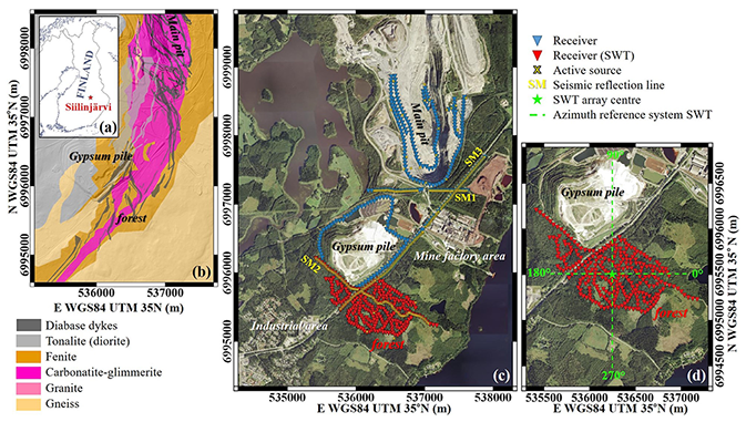
Figure 1Siilinjärvi mine: (a) geographical location; (b) geological map (Yara); (c) active and passive seismic surveys acquired in 2018; (d) zoom on the passive seismic array in the southern area, used for passive surface-wave tomography (SWT). The reference system for azimuth analysis is highlighted in green. Orthophotos available from QGIS plugin QuickMapServices (Kapsi – ortoilmakuva TMS).
The Siilinjärvi deposit is comprised of carbonatite–glimmerite rocks intruded into Archean granitic and gneissic host rocks. An alkali metasomatised fenite halo encircles the carbonatite–glimmerite ore zone. Evenly spaced, predominantly NW–SE- to N–S-striking diabase (i.e., waste rock) dikes crosscut the entire ore body. The thickness of the dikes varies within a range of a few centimeters to several tens of meters (Puustinen, 1971), and most of the known dikes show steep dips, but a significant group of moderately to gently dipping dikes is also known to exist (Mattsson et al., 2019). The dikes intersect each another creating a complex structural pattern, which is later disrupted by N–S-trending shearing along the ore boundaries and by Proterozoic (1.89 Ga) dioritic–tonalitic intrusion in the SW border of the deposit (e.g., Lukkarinen, 2008; Fig. 1b). For future mine planning, besides the more complete characterization of the intricate geostructural setting, further identification and location of sub-horizontally oriented diabase dikes at depth would be crucial. As their locations and extent cannot be reliably predicted based on surface and borehole geological observations, geophysical methods are needed to aid the mapping.
Active and passive seismic data were acquired at Siilinjärvi phosphorus mine in 2018, with a 3D array of randomly distributed stations (Fig. 1c). The deployment design was chosen to respect site and instrumentation logistical constraints and to optimize subsurface illumination (in terms of wavelength and azimuth coverage) in the areas of interest, as further described in Da Col et al. (2020). The seismic array consisted of 578 vertical geophones (10 Hz) connected to wireless stations and almost continuously recorded for 13 d (24 September–6 October). Without any a priori information on the ambient seismic noise spatiotemporal distribution on site, a long acquisition time was selected to maximize the possibility of recording a large variety of useful noise sources. Data gaps occurred mainly during night hours, due to battery discharge. Passive data from all stations were recorded with a sampling rate of 2 ms and stored in 1 min SEGY files. Approximately 800 Gb of seismic traces was acquired. Beside the seismic reflection lines (SM1 to SM3 in Fig. 1b), remaining seismic stations were deployed in three main areas, including the main pit to the north, the gypsum pile located SW, and the southern forest area (Fig. 1c). The latter (Laukansalo, Siilinjärvi) is of crucial importance for future mining activities, since it is known that the mineralization extends to the south from the current main pit. In this area, the 3D random array included 273 stations (in red in Fig. 1c and d) covering approximately 0.8 km2, with an average distance of 50 m between the stations. Passive data recorded in this area were processed to increase depth and resolution of the shear-wave velocity model retrieved for the southern continuation of the mineralization by active SWT (Da Col et al., 2020).
The processing workflow adopted for passive SWT is summarized in Fig. 2. Before the tomographic inversion, a two-step semi-automatic workflow was designed to extract the path-average DCs from the passive data.
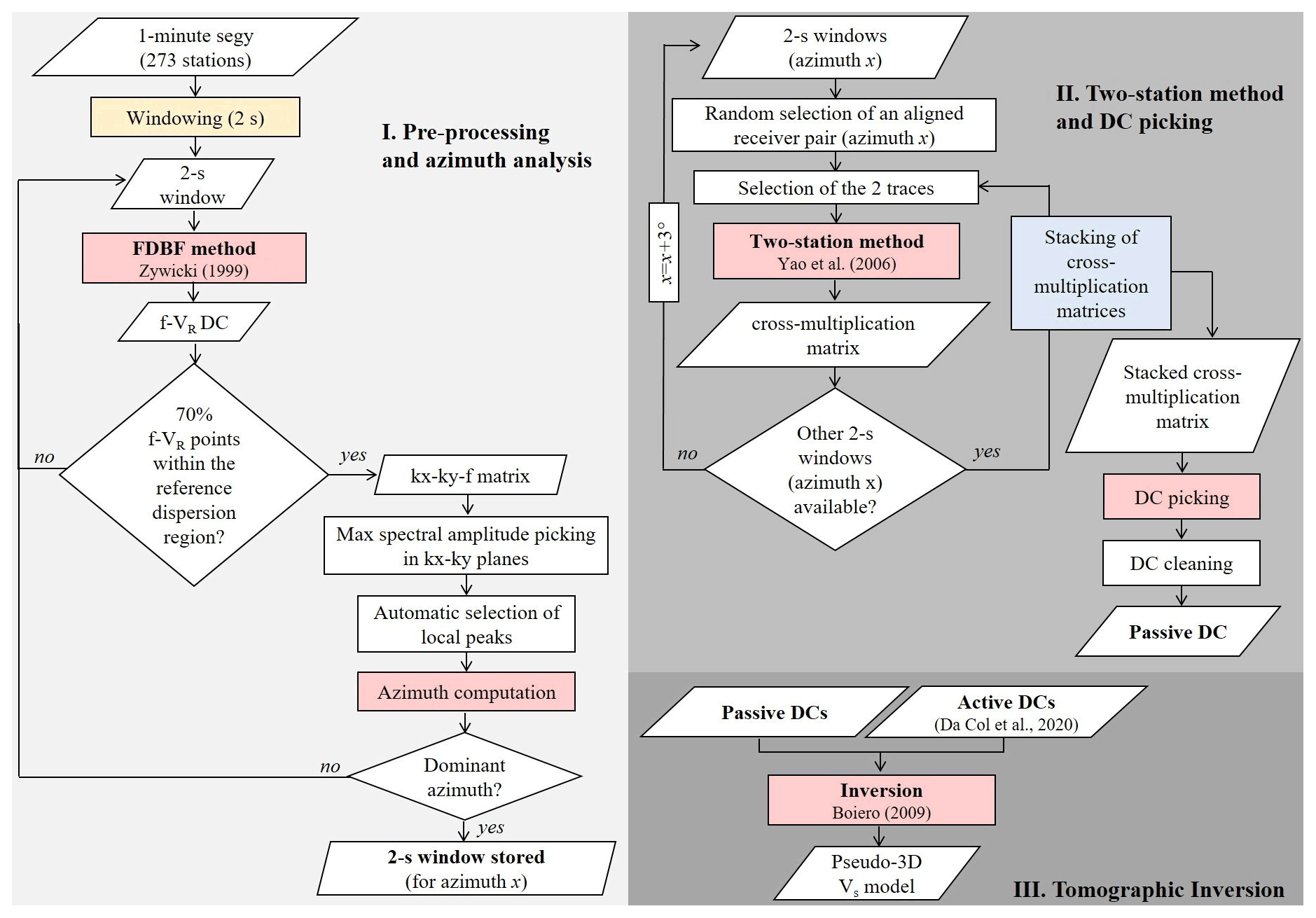
In the pre-processing step (I in Fig. 2), each 1 min SEGY file is windowed in 2 s segments. On each window, the frequency domain beamforming (FDBF) method (Zywicki, 1999) is applied to retrieve frequency–wavenumber (f–kx, ky) power spectral density functions, used to identify dispersive events in the recordings and their direction of propagation. The result is a 3D matrix having kx–ky spectra as planes at the different investigated frequencies (3–20 Hz). This frequency band was chosen to lower the frequency content retrieved from active DCs, generally in the range 7–48 Hz (Da Col et al., 2020). The position of the spectral maximum in each kx–ky plane provides wavenumbers and azimuth of the dominant SWs propagating at that frequency during the 2 s window (Foti et al., 2007). Once the wavenumber modulus is retrieved from kx and ky values, the phase-velocity (VR) of the DC is computed following
where is simply
Further pre-processing steps are summarized in Fig. 3. The DC retrieved from the FDBF method is compared with a reference dispersion region (Fig. 3a), defined on the basis of the velocity ranges of active dispersion curves at the lowest frequencies. If a significant number of DC points are located within the dispersion region, data quality is considered sufficient to continue the computations; otherwise, the time window is rejected. The threshold for window acceptance was chosen by visual inspection of the FDBF DCs retrieved from the 2 s windows of the first day of recording. Considering that all the computed DCs showed phase velocities higher than the active dispersion region at the lowest frequencies and additional noisy points may exist at higher frequencies (e.g., Fig. 3a), 70 % of points within the dispersion region were selected as a good compromise to accept the window for further processing. This threshold is strictly depending on the selection of the active dispersion region, the DC pattern at the lowest frequencies, the analyzed frequency band and the overall data quality, so it may be highly site-dependent and an initial training on the data is recommended for future applications.
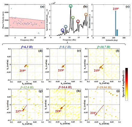
Figure 3Example of frequency-domain beamforming (FDBF) computation on a 2 s window. (a) DC from the FDBF method compared to the reference dispersion region (in red, from active dispersion data, Da Col et al., 2020). (b) Spectral amplitude of the maxima in the kx–ky planes (related to different frequencies). Colored circles refer to the peaks whose kx–ky planes are shown in (d) to (i). (c) Histogram of the azimuth occurrences in the analyzed kx–ky planes. (d–i) kx–ky planes at different frequencies with azimuth computations (degrees counterclockwise from E, green reference system in Fig. 1d).
For the high-quality time windows, the maxima of the kx–ky planes are automatically picked (Fig. 3b). For an automatic random selection of peaks, the azimuth is computed based on its location in the related kx–ky plane (Fig. 3d to i; Okada, 2003; Foti et al., 2007). If there is a dominant azimuth, i.e., consistent among the different frequencies (Fig. 3c), the SW event is considered coherent and the time window is stored in a folder associated to that azimuth value.
This pre-processing procedure is automatically repeated for all the available records. Figure 4a shows the entire recorded data set of 1 min SEGY files analyzed with the pre-processing step. Data gaps occurred predominantly during night hours due to battery discharge. The average amplitude of the ambient seismic noise recorded at the site is variable over time, with higher amplitude in the morning hours of each day, potentially meaning a higher number of SW events recorded by the entire network in these time windows. The number of extracted 2 s time windows containing strong and coherent SW signal is shown in Fig. 4b, with the related azimuth distribution (Fig. 4c). Approximately 7.6 % of the recorded 2 s windows showed a strong SW signal (Fig. 4b). To be consistent with the kx–ky plane orientation, the azimuth distribution is shown in the reference system of Fig. 1d. Nearly 8000 SW events originated at an azimuth around 219∘ (Fig. 4c). More in general, a first cluster of events is located between 200 and 240∘, probably related to the workshop activities located towards W–SW, where industrial machineries are produced and tested (Fig. 1c). A second cluster of events is centered around 50∘, likely related to the factory area located to the NE of the forest, where apatite concentrate is processed on site to produce phosphoric acid and fertilizers (Fig. 1c).
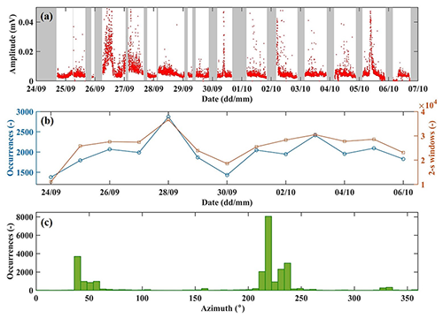
Figure 4(a) Average amplitude of the recorded 1 min ambient seismic noise recordings with indication of data gaps, in grey. (b) Number of 2 s windows with strong SW content (in blue) and total number of 2 s windows recorded during each day of the survey (in orange). (c) Histogram of the azimuthal directions of the selected windows retrieved from the FDBF method (degrees counterclockwise from E, green reference system in Fig. 1d).
In the second processing step (II in Fig. 2), for each azimuth (Fig. 4c), receiver pairs aligned along this direction, with a tolerance of 1∘, are chosen randomly to maximize path length and consequently wavelength distribution. A modified version of the two-station method (as implemented by Yao et al., 2006) is applied to each receiver pair (e.g., Fig. 5a). The receiver traces are cross-correlated frequency by frequency to extract cross-multiplication matrices. This procedure is repeated for the same receiver pair in all the available time windows having the same dominant azimuth. Individual cross-multiplication matrices are then stacked to increase the signal-to-noise ratio. DCs are automatically extracted as the amplitude maxima of the stacked cross-multiplication matrices (Fig. 5b), using the reference dispersion region of active data to guide the picking at the highest frequencies (>10 Hz) and a constant sampling interval equal to 0.5 Hz.

Figure 5Example of DCs obtained by the two-station method. (a) Network geometry and considered receiver pair (green triangles). (b) Stacked cross-multiplication matrix and picked passive DC (black dots). (c) Comparison between passive and active DCs for the same receiver couple.
The comparisons between active and passive DCs for the same receiver pairs (e.g., Fig. 5c) showed matching phase–velocity trend and values in the overlapping frequency/wavelength range. The global passive DC set (1025 curves) retrieved from the picking of the stacked cross-multiplication matrices is shown in Fig. 6 in comparison with the active DCs (433 curves; Da Col et al., 2020). The alignments of passive DC points with different slope, clearly visible at the longer wavelengths (Fig. 6b), are due to the fact that the passive curves were automatically picked at constant frequency intervals (0.5 Hz). The passive curves are generally characterized by wavelengths longer than the active ones, thus enlarging the depth of investigation. The maximum wavelength of the passive DCs (approximately 1200 m) is nearly double the one of the active curves, even though the frequency content in the passive DCs was not significantly lower than the frequencies of the active curves (Fig. 6a). Thanks to the high seismic velocities characterizing the site, even the few additional lower-frequency components present in some of the passive curves resulted in significantly large wavelength increases. The two DC sets were therefore merged to improve the inversion results.
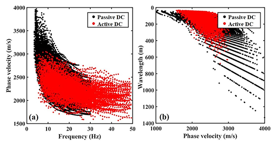
Figure 6Passive (black) and active (red) dispersion curves. (a) Frequency–phase velocity domain. (b) Wavelength-phase velocity domain.
The distribution of the path length and azimuths of all the DCs is shown in Fig. 7. Although we observed peaks in the estimated azimuths around 200–240 and 42–60∘ (Fig. 4c) for the passive data, this did not translate to corresponding peaks in the global DC azimuth coverage. Instead, the distribution of DC azimuths is rather homogeneous, apart from a peak in the 150 and 330∘ direction. This was due to the fact that the cross-correlation matrices, computed for the same receiver pair and different time windows, were stacked, and only one DC was extracted for each receiver pair. Moreover, due to the random geometry of the receivers, several receiver pairs with different path lengths existed at the same azimuth (Fig. 7a) and, therefore, a wide range of path lengths was included in the DC set.
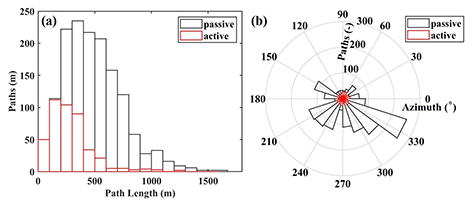
Table 1Discretization and properties of the initial model of the tomographic inversion.

The spatial coverage obtained by adding the passive DCs to the active data set is shown for different depth ranges (assuming a pseudodepth of investigation = half wavelength; Abbiss, 1981). DC coverage is dense in the whole forest area and wavelengths and apparent phase velocities show consistent lateral variability at each wavelength. In the active data only, coverage was lower and limited to a depth of approximately 210 m (Da Col et al., 2020), while acceptable coverage is now retrieved until a depth of approximately 400–500 m.
For the tomographic inversion of the merged data set (III in Fig. 2), the same approach applied to active DCs was followed to retrieve a pseudo three-dimensional shear-wave velocity (VS) model, as described in Boiero (2009); 1D profiles beneath grid points are estimated using damped weighted least square inversion. Horizontal and vertical constraints between neighboring models are set in the regularization matrix to connect VS and thickness information from one model to the surrounding ones. For the spatial discretization, we assumed 420 uniformly distributed grid points, at 44 m from each other. After testing different vertical-discretization dimensions, we concluded that the best DC fitting was achieved assuming seven layers, reaching a maximum depth of 480 m. The adopted initial model is reported in Table 1. A lateral VS constraint of 150 m s−1 for the first four layers and of 500 m s−1 for layers 5–7 was imposed. These were found to be the strongest constraints which did not increase the inversion misfit.
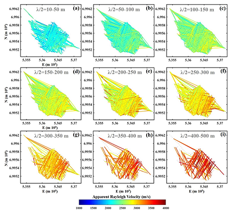
Figure 8Tomographic pseudoslices at selected half-wavelength (pseudodepth) intervals. (a) 10–50 m, (b) 50–100 m, (c) 100–150 m, (d) 150–200 m, (e) 200–250 m, (f) 250–300 m, (g) 300–350 m, (h) 350–400 m, (i) 400–500 m.
The final VS model, obtained after 12 iterations, is shown in Fig. 9 as slices at different depths. In the shallow subsurface (30 m, Fig. 9a), low velocity values (2000–2800 m s−1) are almost homogeneously displayed. Deeper, down to 240 m, the model presents a clear mapping of the carbonatites, characterized by shear-wave velocity values lower than the surrounding rock types, due to their petrophysical properties and fracturing conditions (Da Col et al., 2020). In the same slices, the results highlight several local high-velocity anomalies, which have been earlier interpreted, depending on their location, as the intrusions of diabase dikes within the Siilinjärvi deposit or as the host rock (Fig. 9b to d). These interpretations were already supported by the available surface geological mapping, drilling logs and geological model. The layers between 330 and 480 m (Fig. 9e to g) present a greater extent of high-velocity zones (3300–4000 m s−1) and lower lateral variability.
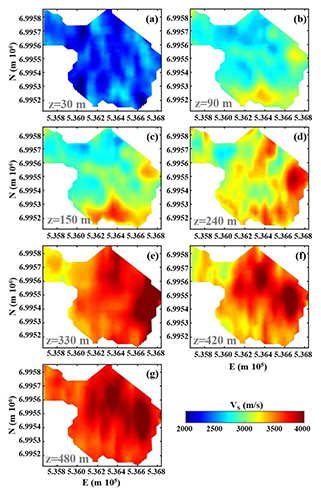
Figure 9Final shear-wave velocity model obtained from active + passive SWT. Model slices at increasing depth: (a) 30 m, (b) 90 m, (c) 150 m, (d) 240 m, (e) 330 m, (f) 420 m, (g) 480 m.
A comprehensive geological interpretation of the final VS model is given in the Discussion section.
The histogram of Fig. 10a shows the misfit between the experimental and theoretical (computed for the inverted model) DC points. The normalized root mean square deviation of the DCs along the analyzed two-station paths is shown in Fig. 10b. The misfit is lower than 12.5 % for more than 75 % of the data points, and there are no zones over the investigated area with concentration of high misfits. The results are therefore acceptable and the estimated DCs are well fitting the experimental ones.
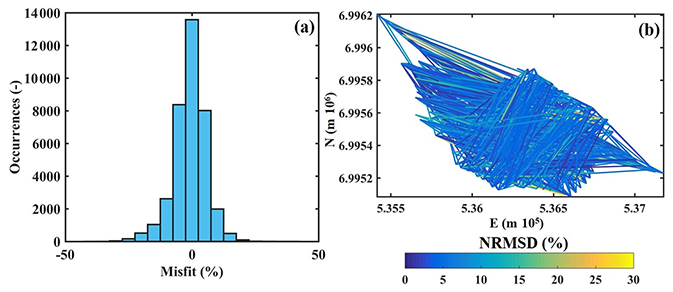
Figure 10Misfit of the active + passive final inversion model. (a) Misfit (in percentage) for each experimentally calculated DC data point. (b) Map of the normalized root mean square deviation of the DCs along the analyzed two-station paths.
To evaluate the resolution of the final model, a checkerboard test was performed. The initial model velocities (Table 1) were perturbed positively and negatively (±8 %) according to the regular pattern of Fig. 11a (squares of 200×200 m). The VS perturbations obtained after the inversion are presented in Fig. 11b. Velocity perturbations at depths 30–330 m are well reconstructed, apart from the south-western portion of the slice at 90 m depth (red box in Fig. 11). Apparently, no reduction in data coverage is depicted in this position (Fig. 8b). This is likely a marginal effect due to the small portion of the square with negative perturbation included within the area covered by the array, as also observable at 240 m depth. At depths 330–480 m, the quality of the inverted checkerboard model reduces, especially at 330 m depth, where the perturbations in the southern portion of the model appear smoothened (blue box in Fig. 11). This can be partially related to a coverage reduction (e.g., Fig. 8h). Nevertheless, the dimensions of the rest of the perturbation blocks in all the other layers are clearly identified in the inverted checkerboard model. Therefore, it can be concluded that the resolution of the experimentally retrieved VS model of Fig. 9 equals, at least, the size of the perturbation blocks of Fig. 11, except for the two zones indicated by the colored boxes.
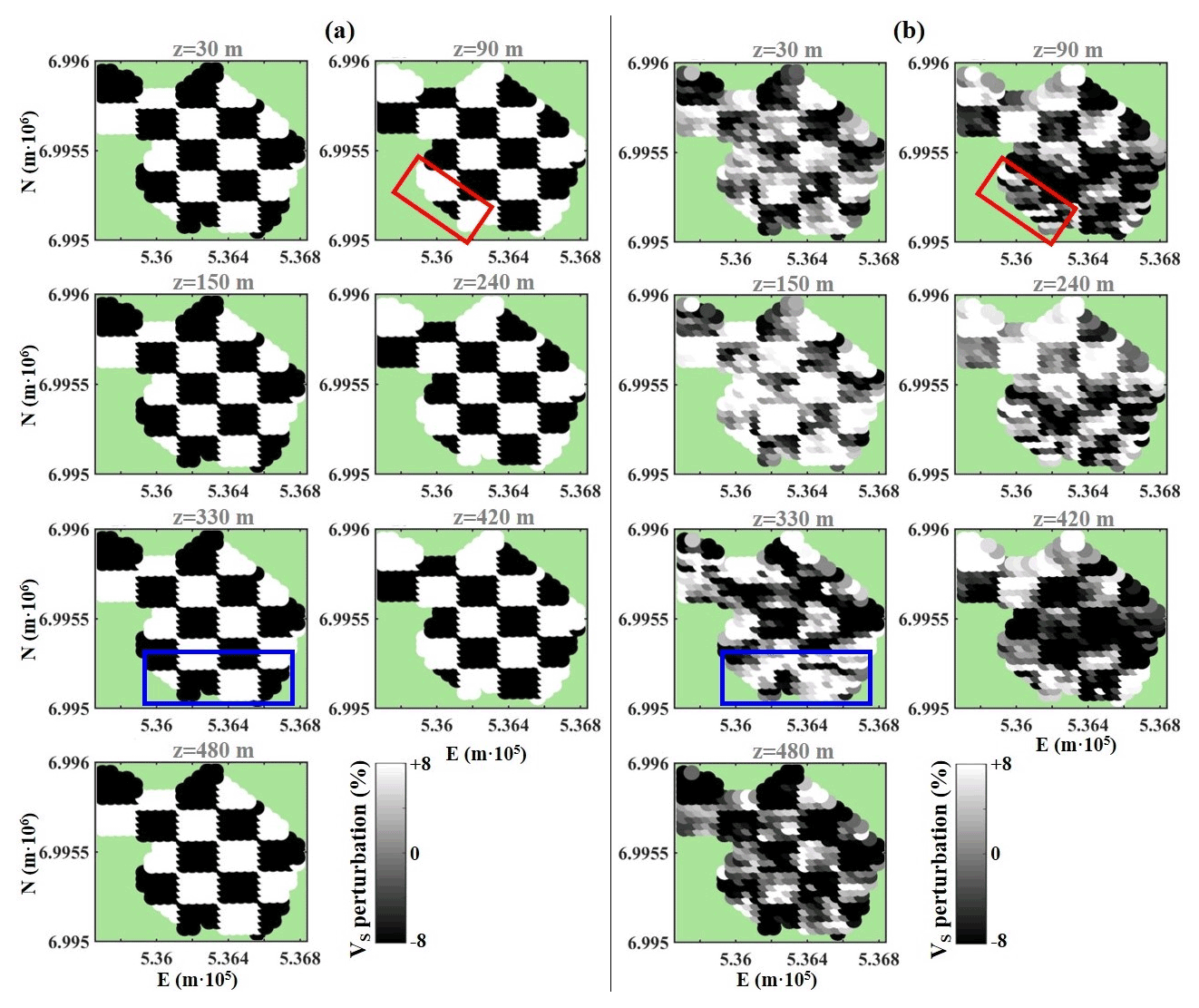
Figure 11(a) True and (b) inverted checkerboard velocity perturbation. The boxes indicate velocity perturbations which could not be accurately recovered.
The combined use of active and passive data led to the reconstruction of a deeper VS model for the area south of the current Siilinjärvi phosphorus mine where a new open pit is planned. Compared to active SWT only, the final model (Fig. 9) highlighted more continuous features which geological interpretation may offer a valuable support for the characterization of the mineralization and future mining plans.
The carbonatite–glimmerite bodies show generally low-velocity signatures as already found in Da Col et al. (2020), but the final velocity distribution now better highlights the general NNE–SSW orientation of the mineralization down to the 240 m depth (Fig. 12b to d). Also the fenite bodies are found to be associated with low-velocity signatures, while surrounding granite and gneiss show the highest VS values at shallow depths (<240 m). No sharp velocity contacts are depicted at the boundaries of the mineralization, but relatively clear arrays of NNE–SSW discontinuities coincide with diabase dikes and shear zones as modeled by Yara (Fig. 12a) and can be used to delineate the margins of the mineralization (I in Fig. 12c). In particular, the western contact is visible at all depths, and it is more distinct than the eastern margin. The contrasting character of the margins is in line with the observations on DDH data, where the eastern contact is found to be gradational and defined by alternating layers of carbonatite-glimmerite, fenite and tonalite. In the eastern area of investigation, the NNE–SSW discontinuities and transitions in the seismic velocity signatures can be used to improve the delineation of the contacts between fenite and granite–gneiss (IV). Some structural embayments along the fenite–granite/gneiss contact are possible, as highlighted by the different dashed pattern along line IV at the depth of 150 m (Fig. 12c). Such geometry is compatible with the overall irregular thickness of the fenite within the ground surface level geological maps (Fig. 1b). A sharp increase in velocity is seen from the depth of 240 m downwards, but with no direct linkage to known geological features. The increasing velocities are likely consistent with a reduction in weathering and fracturing from the shallow subsurface downwards. However, this also matches the fabric of stronger reflectivity segments on the 2D reflection seismic sections (SM1 and SM2 in Fig. 1c), possibly originating from contacts to diabase dikes.
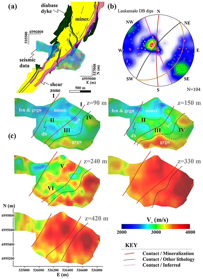
Figure 12Geological interpretation of the final S-wave velocity model. (a) Overview of the area of the seismic investigation and the geological model of the site (from Yara). (b) Lower hemisphere stereographic projection of poles to the diabase contacts available from oriented diamond drill hole data. The great circles represent mean orientations of the four recognized diabase dike sets. (c) Level images of the seismic data with geological interpretation of the main lithological boundaries. miner. – carbonatite–glimmerite mineralization, fen – fenite, db – diabase and grgn – granite–gneiss.
In the model slices 90–240 m, discontinuous higher-velocity areas within the mineralization, and to a lesser degree in fenite, loosely define a structural network that we infer to represent diabase dikes (II, III, V and VI). In particular, feature II does not directly correlate with any known diabase dike set but could result from the interplay of different dike sets, comprising also the strictly horizontal dikes presently included in the gently ESE-dipping set (orange in Fig. 12b). Feature III may correlate with the sub-vertical NNW–SSE trending dike set (magenta in Fig. 12b). The orientation of thin diabase dikes found in some DDH is compatible with V and VI at 240 m depth, as well as with the larger dikes bounding the mineralization.
At deeper levels, the NNE–SSW-trending western margin of the high-velocity material remains the most visible feature, in agreement with the regional trend and the dominant population of diabase dikes, while no internal structures can be recognized in the mineralization from the seismic results. A parallel (NNE–SSW) but less distinct seismic “low” coincides with the fenite bounding the mineralization to the E.
In general, decametric geostructural features, with a size compatible with the checkerboard perturbations of Fig. 11, are clearly observable in the SWT results. Smaller-scale individual dikes and other local geological features shown by DDH data and observations in the Siilinjärvi main pit, further in the north, are below the expected resolution.
The application of combined active and passive SWT provided a high-resolution deep seismic velocity model for the southern continuation of the Siilinjärvi phosphate deposit, on which new mining activities can be potentially focused in the future. We proposed a semi-automatic workflow for the extraction of the path-average DCs from ambient noise data recorded on site in 2018. The pre-processing steps allow the extraction of the time windows containing sufficient SW energy, minimizing the time and computational costs of the subsequent processing steps. The distribution of azimuths provides information about the noise sources and allows for the application of the two-station method, which requires the receivers to be in-line with the source. The method is almost fully automatic, apart from an initial calibration of the pre-processing criteria (i.e., thresholds to compare passive DC points and the reference active dispersion region and to declare that a dominant azimuth is present in the window) and a quality control of the picked DCs on a training data set. However, due to the large size of the data set (almost 800 Gb), the pre-processing computations required around 3 weeks, running in parallel on a 10-core workstation. Including only the accepted time windows, the data set was downsized to approximately 61.5 Gb. The DCs obtained by the proposed workflow are comparable to the ones obtained from active data in the overlapping frequency range, thus supporting the reliability of the results. Moreover, it was shown that passive data contain more information about the deeper subsurface portions, increasing the investigation depth and, therefore, opening the possibility of mapping the target at depth. Combined with the active DCs, they provided high-resolution SWT results down to 480 m depth. The time required for the two-station processing, stacking and semi-automatic DC picking was approximately 1 week, while the tomographic inversion required approximately 6.5 h on the same 10-core workstation. The final velocity model was validated through interpretation of the main seismic signatures in comparison with the available geostructural data. Results confirm the southern extension of the carbonatite–glimmerite deposits and help in constraining the geometry of the mineralization and in unraveling the intricate relationships with the host rocks and the major intruding dikes. This model can be used to guide future drilling efforts for a detailed characterization of the mineralization in the area.
This successful application has proven that the use of passive data within SWT is a promising, cost-effective and sustainable tool for deep mineral exploration, overcoming the need for active seismic sources.
Code and data were developed and acquired within the EU H2020 project Smart Exploration (grant agreement no. 775971) and may be available by contacting the corresponding author.
CC and MP worked on SW passive data processing, with coordination and supervision of LVS. TK, PS, EK and MS worked on the geological interpretation of the seismic results. MP and EK contributed to seismic data acquisition. CC wrote the original paper draft, with contributions from all the authors.
The contact author has declared that neither they nor their co-authors have any competing interests.
Publisher’s note: Copernicus Publications remains neutral with regard to jurisdictional claims in published maps and institutional affiliations.
This article is part of the special issue “State of the art in mineral exploration”. It is a result of the EGU General Assembly 2020, 3–8 May 2020.
We thank Yara Suomi Oy for the access to geological models and their overall hospitality. The data were acquired using combined seismic equipment of Uppsala University and Geopartner Sp. z.o.o., for which we are thankful. We thank everyone who participated in the survey, especially the master and PhD students, whose support was vital during the fieldwork. We are grateful to Federico Da Col for starting this work and whose results on the active data provided solid basis for the continuation of the study.
Smart Exploration has received funding from the European Union's Horizon 2020 research and innovation programme under grant agreement no. 775971.
This paper was edited by Juan Alcalde and reviewed by two anonymous referees.
Abbiss, C. P.: Shear wave measurements of the elasticity of the ground, Geotechnique, 31, 91–104, https://doi.org/10.1680/geot.1981.31.1.91, 1981.
Boiero, D.: Surface wave analysis for building shear wave velocity models, PhD Thesis, Politecnico di Torino, Torino, Italy, 2009.
Bussat, S. and Kugler, S.: Recording noise – Estimating shear-wave velocities: Feasibility of offshore ambient-noise surface-wave tomography (answt) on a reservoir scale, SEG Technical Program Expanded Abstracts 2009, 1627–1631, https://doi.org/10.1190/1.3255161, 2009.
Colombero, C., Comina, C., and Socco, L. V.: Imaging near-surface sharp lateral variations with surface-wave methods – Part 1: Detection and location, Geophysics, 84, EN93–EN111, https://doi.org/10.1190/geo2019-0149.1, 2019.
Da Col, F., Papadopoulou, M., Koivisto, E., Sito, Ł., Savolainen, M., and Socco, L. V.: Application of surface-wave tomography to mineral exploration: A case study from Siilinjärvi, Finland, Geophys. Prospect., 68, 254–269, https://doi.org/10.1111/1365-2478.12903, 2020.
Decrée, S. and Robb, L.: Developments in the Continuing Search for New Mineral Deposits, Eos, 100, https://doi.org/10.1029/2019EO128347, 2019.
Eaton, D. W., Milkereit, B., and Salisbury, M. H. (Eds.): Hardrock Seismic Exploration, Society of Exploration Geophysicists, Tulsa, USA, https://doi.org/10.1190/1.9781560802396, 2003.
Foti, S., Comina, C., and Boiero, D.: Reliability of combined active and passive surface wave methods, Rivista Italiana di Geotecnica, 41, 39–47, 2007.
Hollis, D., McBride, J., Good, D., Arndt, N., Brenguier, F., and Olivier, G.: Use of ambient noise surface wave tomography in mineral resource exploration and evaluation, SEG Technical Program Expanded Abstracts 2018, 1937–1940, https://doi.org/10.1190/segam2018-2998476.1, 2018.
Kennett, B. L. N. and Yoshizawa, K.: A reappraisal of regional surface wave tomography, Geophys. J. Int., 150, 37–44, https://doi.org/10.1046/j.1365-246X.2002.01682.x, 2002.
Lehujeur, M., Vergne, J., Maggi, A., and Schmittbuhl, J.: Ambient noise tomography with non-uniform noise sources and low aperture networks: Case study of deep geothermal reservoirs in northern Alsace, France, Geophys. J. Int., 208, 193–210, https://doi.org/10.1093/gji/ggw373, 2017.
Lukkarinen, H.: Pre-Quaternary rocks of the Siilinjärvi and Kuopio map-sheet areas, Geological map of Finland 1 : 100 000, Explanation to the maps of Pre-Quaternary rocks, Sheets 3331 Siilinjärvi and 3242 Kuopio, Espoo, 2008.
Lynch, R., Hollis, D., McBride, J., Arndt, N., Brenguier, F., Mordret, A., Boué, P., Beaupretre, S., Santaguida, F., and Chisolm, D.: Passive seismic ambient noise surface wave tomography applied to two exploration targets in Ontario, Canada, SEG Technical Program Expanded Abstracts 2019, 5390–5392, https://doi.org/10.1080/22020586.2019.12073192, 2019.
Malehmir, A., Heinonen, S., Dehghannejad, M., Heino, P., Maries, G., Karell, F., Suikkanen, M., and Salo, A.: Landstreamer seismics and physical property measurements in the Siilinjärvi open-pit apatite (phosphate) mine, central Finland, Geophysics, 82, B29–B48, https://doi.org/10.1190/geo2016-0443.1, 2017.
Martins, J. E., Weemstra, C., Ruigrok, E., Verdel, A., Jousset, P., and Hersir, G. P.: 3D S-wave velocity imaging of Reykjanes Peninsula high-enthalpy geothermal fields with ambient-noise tomography, J. Volcanol. Geoth. Res., 391, 106685, https://doi.org/10.1016/j.jvolgeores.2019.106685, 2020.
Mattsson, H. B., Högdahl, K., Carlsson, M., and Malehmir, A.: The role of mafic dykes in the petrogenesis of the Archean Siilinjärvi carbonatite complex, east-central Finland, Lithos, 342, 468–479, https://doi.org/10.1016/j.lithos.2019.06.011, 2019.
O'Brien, H., Heilimo, E., and Heino, P.: The Archean Siilinjärvi carbonatite complex, edited by: Maier, W. D., Lahtinen, R., and O'Brien, H., Mineral Deposits of Finland, Elsevier, 327–343, https://doi.org/10.1016/B978-0-12-410438-9.00013-3, 2015.
Okada, H.: The microtremor survey method, Geophysical monograph series, 12, SEG, Tulsa, USA, https://doi.org/10.1190/1.9781560801740, 2003.
Papadopoulou, M., Da Col, F., Mi, B., Bäckström, E., Marsden, P., Brodic, B., Malehmir, A., and Socco, L. V.: Surface-wave analysis for static corrections in mineral exploration: A case study from central Sweden, Geophys. Prospect., 68, 214–231, https://doi.org/10.1111/1365-2478.12895, 2020.
Park, C. B., Miller, R. D., Ryden, N., Xia, J., and Ivanov, J.: Combined use of active and passive surface waves, J. Environ. Eng. Geoph., 10, 323–334, https://doi.org/10.2113/JEEG10.3.323, 2005.
Planès, T., Obermann, A., Antunes, V., and Lupi, M.: Ambient-noise tomography of the Greater Geneva Basin in a geothermal exploration context, Geophys. J. Int., 220, 370–383, https://doi.org/10.1093/gji/ggz457, 2020.
Puustinen, K.: Geology of the Siilinjärvi carbonatite complex, eastern Finland, Geological Survey of Finland, Bulletin de la Commission Géologique de Finlande, 249, 43 pp., 1971.
Ritzwoller, M. H. and Levshin, A. L.: Eurasian surface wave tomography: Group velocities, J. Geophys. Res.-Sol. Ea., 103, 4839–4878, 1998.
Sabra, K. G., Gerstoft, P., Roux, P., Kuperman, W., and Fehler, M. C.: Surface wave tomography from microseisms in Southern California, Geophys. Res. Lett., 32, L14311, https://doi.org/10.1029/2005GL023155, 2005.
Shapiro, N. M., Campillo, M., Stehly, L., and Ritzwoller, M. H.: High-resolution surface-wave tomography from ambient seismic noise, Science, 307, 1615–1618, 2005.
Socco, L. V. and Strobbia, C.: Surface-wave method for near-surface characterization: a tutorial, Near Surf. Geophys., 2, 165–185, https://doi.org/10.3997/1873-0604.2004015, 2004.
Tichomirowa, M., Grosche, G., Götze, J., Belyatsk, B. V., Savva, E. V., Keller, J., and Todt, W.: The mineral isotope composition of two Precambrian carbonatite complexes from the Kola Alkaline Province–Alteration versus primary magmatic signatures, Lithos, 91, 229–249, 2006.
Yao, H., van der Hilst, R. D., and De Hoop, M. V.: Surface-wave array tomography in SE Tibet from ambient seismic noise and two-station analysis – I. Phase velocity maps, Geophys. J. Int., 166, 732–744, https://doi.org/10.1111/j.1365-246X.2006.03028.x, 2006.
Yin, X., Xu, H., Wang, L., Hu, Y., Shen, C., and Sun, S.: Improving horizontal resolution of high-frequency surface-wave methods using travel-time tomography, J. Appl. Geophys., 126, 42–51, https://doi.org/10.1016/j.jappgeo.2016.01.007, 2016.
Zywicki, D. J.: Advanced signal processing methods applied to engineering analysis of seismic surface waves, PhD Dissertation, Georgia Institute of Technology, Atlanta, USA, 1999.