Reference seismic crustal model of the Dinarides

Continental collision zones are structurally one of the most heterogeneous areas intermixing various different units within a relatively small space. A good example of this is the Dinarides, a mountain chain situated in the central Mediterranean, where thick carbonates cover older crystalline basement units and remnants of subducted oceanic crust. This is further complicated by the highly variable crustal thickness ranging from 20 to almost 50 km. In terms of spatial extension, this area is relatively small but covers tectonically differentiated domains making, any seismic or geological analysis complex, with significant challenges in areas that lack seismic information on crustal structure.

Presently there is no comprehensive 3D crustal model of the Dinarides (and surrounding areas). Using the compilations of previous studies and employing kriging interpolation, we created a vertically and laterally varying crustal model defined on a regular grid for the wider area of the Dinarides, also covering parts of Adriatic Sea and the SW part of the Pannonian Basin. The model is divided by three interfaces, Neogene deposit bottom, carbonate rock complex bottom and Moho discontinuity, with seismic velocities (P and S waves) and density defined at each grid point. To validate the newly derived model, we calculated travel times for an earthquake recorded on several seismic stations in the Dinarides area. The calculated travel times show significant improvement when compared to the simple 1D model used for routine earthquake location in Croatia.

The model derived in this work represents the first step towards improving our knowledge of the crustal structure in the complex area of the Dinarides. We hope that the newly assembled model will be useful for all forthcoming studies (e.g., as a starting model for seismic tomography, as a model for earthquake simulations) which require knowledge of the crustal structure.

1 Introduction

The first seismic investigation done in the wider Dinarides region can be traced to Andrija Mohorovičić's famous discovery of the boundary between the Earth's crust and mantle (Mohorovičić, 1910). The earliest deep seismic sounding experiments investigating the crustal structure beneath the Dinarides were conducted in the 1960s (Dragašević and Andrić, 1975; Aljinović, 1983; Aljinović et al., 1987). The most important results from those early investigations were about the thickness of the upper crust (Aljinović, 1983). In more recent times, there was another set of active seismic experiments. The ALP 2002 (Brückl et al., 2007) focused on the investigation of the eastern Alps but also covered the northernmost part of the Dinarides and the Pannonian Basin. As part of the same international experiment, Šumanovac et al. (2009) modeled velocities in the crust and uppermost mantle from the measurements taken along the Alp07 profile located at the crossing between the NW Dinarides and SW margin of the Pannonian Basin. The results from the Alp07 profile were later extended by several studies, including gravimetric modeling, P-wave receiver function analysis and local earthquake tomography (Šumanovac, 2010; Šumanovac et al., 2016; Orešković et al., 2011; Kapuralić et al., 2019), covering only the NW part of the Dinarides and SW part of the Pannonian Basin. These studies reported a two-layer crust in the area of the Dinarides and a one-layer crust in the area of the Pannonian Basin.

The first Moho map of the Dinarides was compiled by Skoko et al. (1987), utilizing gravimetric data from that area. Similarly, Šumanovac (2010) used results from active seismic experiments (Alp07) to calibrate gravimetric data and get a more accurate map of Moho depths in the region. Stipčević et al. (2011) were the first to use direct seismic measurements in the central and southern Dinarides, extending the analysis of Moho depths to that region. For this, they employed the P-wave receiver function (PRF) method and by modeling it found an intra-crustal reflector in the area of the Internal Dinarides. Stipčević et al. (2020) extended the PRF analysis by including significantly more stations and created the map of Moho depths beneath the Dinarides. In that expanded receiver function study, Stipčević et al. (2020) report significantly thicker crust in the area of the southern Dinarides compared to the previous studies.

Complementary to the crustal exploration there have also been some recent investigations of the uppermost mantle. Using the S-wave receiver functions (SRFs) Belinić et al. (2018) mapped the lithosphere–asthenosphere boundary (LAB) under the Dinarides. The most interesting feature of that LAB map is the lack of deep lithospheric root beneath the central Dinarides, which was interpreted as thinning of the lithosphere due to possible lithospheric mantle delamination. Two years later, there was a complementary study by Belinić et al. (2020), using Rayleigh wave tomography in order to obtain an upper-mantle S-wave velocity model for the greater Dinarides area. Similar to their first work, the authors reported a missing deep lithospheric root in the area of the central Dinarides and a high-velocity uppermost mantle anomaly visible in the southern Dinarides.

From this short outline of the main geophysical investigations done in the wider Dinarides area it is obvious that the crustal structure of the region is fairly complex with quite a long history of geophysical exploration. Despite this, there has never been an attempt (as far as we know) to combine these results in order to create an extensive regional 3D crustal model for the Dinarides. The area was covered by the global- and continental-scale models, but the authors of these studies pointed out the lack of available data in the Dinarides area (e.g., Grad et al., 2009; Molinari and Morelli, 2011; Artemieva and Thybo, 2013). Note that those continental-scale models were published prior to some of the investigations whose results were used for derivation of our crustal model. Regional-scale crustal models are an important factor in all seismic studies relying on waveform modeling and seismic wave travel time inversion. This is especially exacerbated in areas with complex crustal structure such as the Dinarides. Therefore, it is necessary to assemble a comprehensive, ready-to-use model based on all the available results.

In this study we focus on the crust and include all the data regarding crustal structure available to us in a 3D model covering the area of the Dinarides. The aim is to create a vertically and laterally varying crustal model defined on a regular grid for the wider area of the Dinarides. This model will be a good starting point for both body and surface wave tomography studies and provide an excellent base model for local and regional physics-based earthquake shaking scenarios. Besides the seismic velocity as the main parameter describing the crustal structure, we also include existing data on the Moho discontinuity depth and the approximate thickness of a carbonate rock layer (the carbonate rock complex, CRC) in the Dinarides. Even though our crustal model is focused on the Dinarides, part of it also covers the SW margin of the Pannonian Basin and Adriatic Sea (Fig. 1).

2 Tectonic and geological setting

The Alpine–Carpathian–Dinaridic–Albanide–Hellenic orogenic system is a part of a circum-Mediterranean orogenic system. Encircling the Neogene Pannonian Basin System (PBS), this orogenic system is constructed of tectonostratigraphic units derived from both the Adriatic microplate and the European plate that were separated by the Neotethys Ocean (Schmid et al., 2008, 2020, and references therein). Tectonic units were amalgamated by fold-and-thrust systems of different polarity facing either the European foreland (e.g., western and eastern Alps and Carpathians) or the Adriatic foreland (e.g., southern Alps, Dinarides, Albanides, Hellenides) as a result of a change in subduction polarity between the European plate and the Adriatic Microplate (Schmid et al., 2008, 2020; Ustaszewski et al., 2008).

The tectonic evolution of these large orogenic systems, i.e., Dinarides sensu lato, started with the Triassic (ca. 220 Ma) opening of the Neotethys oceanic embayment between the African and Eurasian plates. The Neotethys Ocean continued spreading during the Late Triassic and Early to Mid-Jurassic, being interrupted only by intra-oceanic subduction of the western Vardar oceanic domain and ophiolite obduction onto the eastern margin of the Adriatic Microplate (see Schmid et al., 2020, for details). According to Schmid et al. (2008), the Neotethys Ocean, i.e., the eastern Vardar oceanic domain, remained open through the Late Jurassic–Cretaceous period (see Ustaszewski et al., 2009, and references therein).

The final closure of the Neotethys oceanic realm coincided with the collision of the Adria Microplate and the European foreland during the Late Cretaceous–early Paleogene (Schmid et al., 2020, and references therein) that initiated formation of the Dinarides (Środoń et al., 2018). During the middle Eocene–Oligocene, the regional NE–SW-oriented compression caused NE-directed continental subduction and formation of complex fold-and-thrust sheets in the Dinaridic region due to SW-directed thrusting of Adria-derived units, whereas in the internal Dinaridic domains, E–W-oriented compression caused the formation of the W-directed thrusting of the Tisza mega-unit over the internal parts of the Dinarides (e.g., Handy et al., 2019; Schmid et al., 2020; Balling et al., 2021; and references therein). Continuous convergence of the Adria indenter towards the European foreland in the late Oligocene–Early Miocene further contributed to nappe stacking and thrusting in the Alps and Dinarides, but it also accommodated ca. 400 km of E-directed orogen-parallel lateral extrusion of the ALCAPA block (including the eastern Alps, western Carpathians and Transdanubian ranges north of Lake Balaton) and active “back-arc-type” extension in the PBS (Royden and Horváth, 1988; Ratschbacher et al., 1991a, b; Frisch et al., 1998; Fodor et al., 1998; Tari et al., 1999; Csontos and Vörös, 2004; Horváth et al., 2006; Cloetingh et al., 2006; Schmid et al., 2008).

With dimensions 80–200 km wide and nearly 700 km long, the Dinarides are a fold-and-thrust orogenic belt constructed from thrust sheets divided into internal and external tectonic domains (see Fig. 1). The lithological succession in the Internal Dinarides is characterized by units that comprise passive margin ophiolitic successions and pelagic-derived sedimentary rocks, while the External Dinarides are dominated mainly by shallow marine carbonate platform deposits that in places reach 8000 m in thickness (Vlahović et al., 2005). Due to paleogeographic differences and tectonic complexity, the Dinaridic lithological succession is spatially highly varied in its thickness and exposure (Vlahović et al., 2005; Schmid et al., 2020; Balling et al., 2021).

The oldest rocks cropping out in the External Dinarides are Carboniferous to Middle Triassic siliciclastic–carbonate deposits accumulated along the Gondwanian passive continental margin, which due to regional extensional tectonics marked by Middle Triassic volcanism differentiated the area, thus forming isolated shallow marine carbonate platforms (Vlahović et al., 2005). Through the Middle Triassic–Cretaceous time span, carbonate platforms in the region were surrounded by deeper marine areas and characterized by mostly continuous shallow marine carbonate deposition, though the last extensional phase in the Toarcian resulted in a disintegration into several smaller platforms, including the Adriatic Carbonate Platform, Apenninic Carbonate Platform and Apulian Carbonate Platform (Vlahović et al., 2005, and references therein). During the 120 Myr of existence of the Adriatic Carbonate Platform (AdCP), i.e., from the Early Jurassic to the Late Cretaceous (locally even to the early Paleocene; Cvetko Tešović et al., 2020), the thickness of deposited carbonate successions reached between 3500 and 5000 m (Vlahović et al., 2005, and references therein). The AdCP deposition ended due to regional emergence in the Late Cretaceous–Paleogene, which was linked and enhanced by tectonic deformations and continent collision of the Adria Microplate and the European foreland yielding deposition of synorogenic turbiditic deposits (“flysch”) in newly formed foreland basins (Vlahović et al., 2005; Schmid et al., 2008; and references therein). The final uplift of the Dinarides took place from the middle Eocene to Oligocene (Dinaric phase; see Schmid et al., 2008; Balling et al., 2021; and references therein).

3 Modeling approach

Generally, the new model is defined as a one-layered crust with laterally and vertically variable parameters (seismic velocities and density). This was done due to the fact that only information about crustal thickness was available for the whole investigated region. Nevertheless, during data collection and integration within the new model we realized that the Neogene deposits in the Pannonian Basin make up a very thick and distinct layer, and just incorporating it into a one-layered model would be an oversimplification. In light of the Pannonian Basin sedimentary complex being significantly different from the rest of the crust, we included a Neogene deposit layer on top of a laterally and vertically varying crust. The same goes for the Paleozoic–Paleogene carbonates in the Adriatic–Dinarides region as there are numerous studies indicating distinct reflections from the bottom of the CRC in the seismic-reflection studies (Dragašević and Andrić, 1975; Aljinović, 1983; Aljinović et al., 1987). Given that there were no data on any of the parameters in this layer (velocity or density), we only included the CRC bottom depth in our model. The velocity and density of the CRC were not interpolated separately but were interpolated using the same input velocity (and density) data we had available for the rest of the crust. This choice seems reasonable, since each of the profiles used crosses the part of the investigated area covered with carbonates and samples its features, even though none of the studies used explicitly interpreted carbonates as a separate layer.

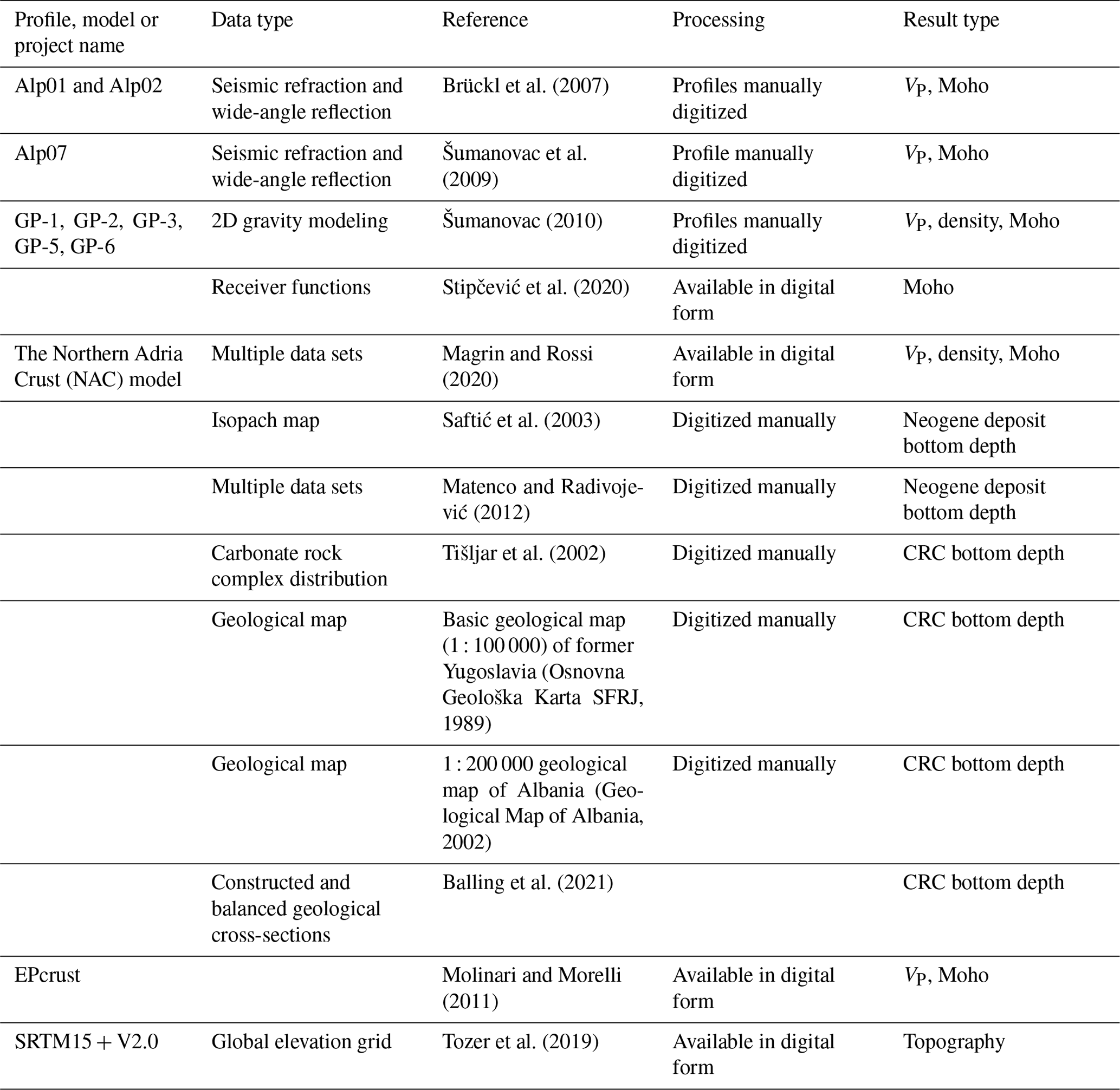
To compile the data for the new crustal model, we used all available and published results on seismic and geologic structure of the crust and uppermost mantle. Some of them were not available in a digital form (mostly the studies published before 2010) and had to be digitized manually. The data sets used are very diverse: two 3D crustal models (one consisting of a two-layered crust with interface depth information, while the other had a single-layered crust), several 2D interface maps (Moho depths and Neogene deposits maps), three seismic-refraction and wide-angle-reflection profiles (which were the basic source for velocity data) and five gravimetric profiles. Coverage of the data sets used to compile the 3D crustal model of the Dinarides is shown in Fig. 1, and details are listed in Table 1. The exact locations of data points used are shown in Appendix B.

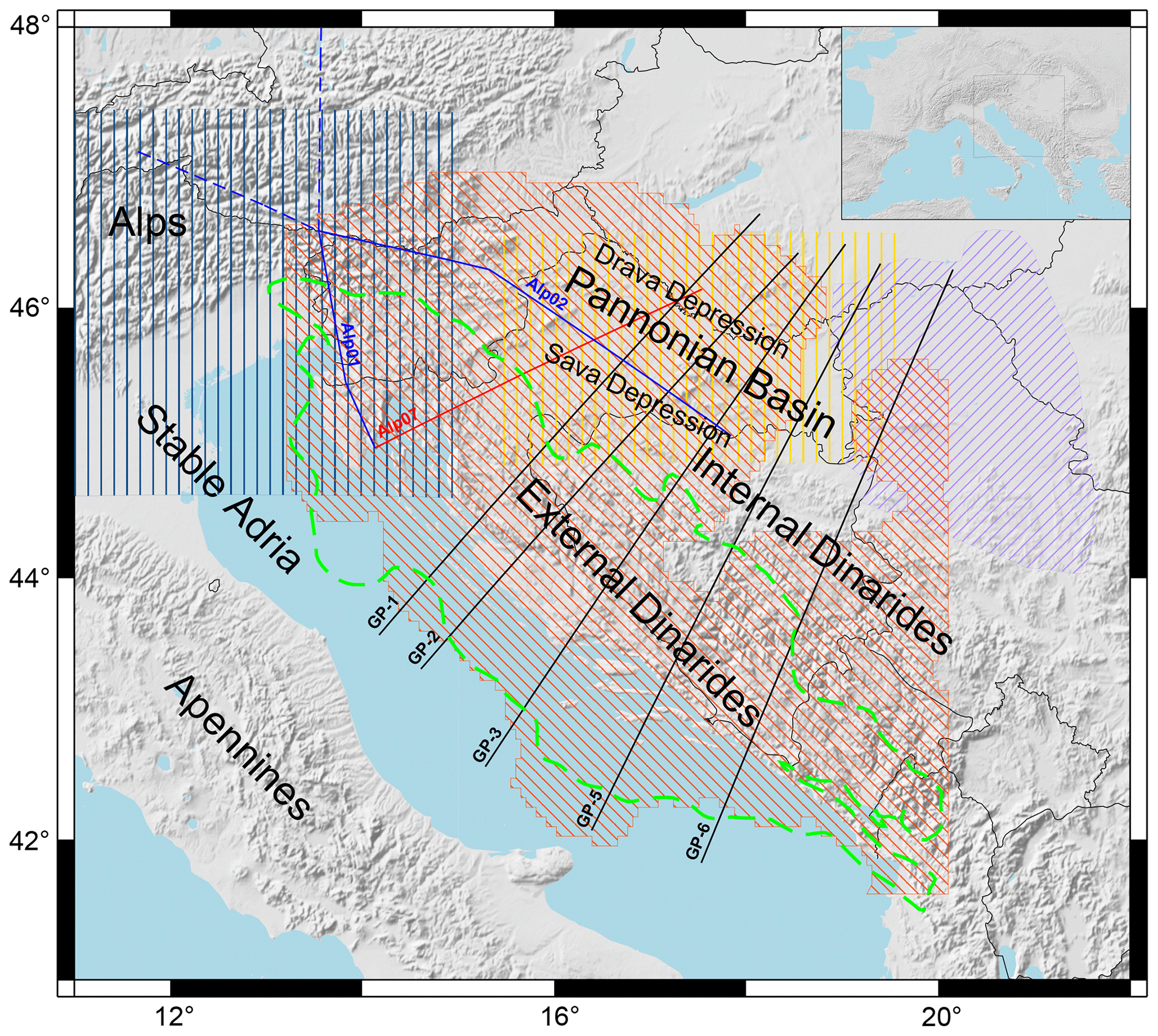
Figure 1 Compilation of data used in this study. Blue lines mark the positions of Alp01 and Alp02 profiles (Brückl et al., 2007); only the full line parts are used in the study. The red line is the position of the Alp07 profile (Šumanovac et al., 2009). Black lines are the positions of gravimetric profiles GP-1 to GP-6 (Šumanovac, 2010). The shaded orange area shows Moho depth data coverage from the receiver function study of Stipčević et al. (2020). The vertically shaded blue area is the NAC model (Magrin and Rossi, 2020). The shaded yellow area shows the extent of Saftić et al. (2003) data on the Pannonian Basin Neogene deposits, and the shaded purple area shows the extent of data on the Pannonian Basin Neogene deposits from Matenco and Radivojević (2012). The dashed green line marks the extension of the AdCP carbonate rocks from Tišljar et al. (2002). The sources of the data shown in this map are listed in Table 1.

Table 1 List of the data sources used for the Dinarides crustal model. V_P: P-wave velocity.

The interpolation of model parameters was done using the kriging method (for details see Appendix C), which is formulated for the estimation of continuous spatial attributes (e.g., depth to Moho interface) at an unknown site, using the limited set of data from sampled sites. Since kriging requires Cartesian coordinates, we transformed the data to the ETRS89-extended and LAEA Europe Cartesian coordinate system (Annoni et al., 2003), which is defined on the entire investigated area. The transformations were done using the pyproj package (Snow et al., 2021). Kriging interpolation was done using the gstat package (Pebesma, 2004). Interface data were interpolated on a regular 5 km × 5 km grid, and the velocity and density were interpolated on a slightly more complex grid: the horizontal grid is the same as for the interfaces (5 km × 5 km), but the vertical spacing changes with depth (in the first 10 km of depth, the spacing is 0.5 km; between depths of 10 and 20 km, vertical spacing is 1 km; and at greater depths, vertical spacing is 2.5 km). This scheme was used to account for better sampling and more heterogeneous upper crust.

Initially, we specified a relatively large area between 10 and 22^∘ E and 39 and 48^∘ N as the starting region of investigation. We performed interpolation in the entire initial region for each interface separately. As some of the areas in the initial region were not covered by data points (see Appendix B) the final model area was reduced based on the Moho discontinuity depth errors in combination with lower-uncertainty areas of the V_P model. The final model covers roughly the area between 13 and 20^∘ E and 42 and 47^∘ N.

Kriging does not allow multiple values at a single point in space (i.e., there is no overlapping), so all overlapping data from various sources were processed before the interpolation. We tried to reduce subjectivity as much as possible and therefore included known and estimated variances into the data processing. In the case of data overlapping, we calculated the value which was used for interpolation (depth for interfaces or velocity and density for layer parameters) at the given point as a weighted mean of multiple values from different sources, with inverse of variances used as weights:

$${\widehat{d}}_{\mathrm{m}}={\displaystyle \frac{\sum _i\frac{\mathrm{1}}{{\mathit{\sigma }}_i^{\mathrm{2}}}{d}_{\mathrm{m},i}}{\sum _i\frac{\mathrm{1}}{{\mathit{\sigma }}_i^{\mathrm{2}}}}},$$

where d_m,i is the value at point i, and ${\mathit{\sigma }}_i^{\mathrm{2}}$ is variance at point i.

We also included error estimates in the final model. To calculate the total error in the model, we followed the procedure applied by Magrin and Rossi (2020) for the derivation of the NAC model. With the assumption of Gaussian distribution of errors, the total variance of the model is the sum of two terms: the variance of the input data and the variance from the interpolation itself. The interpolation variance term was provided by the gstat package along with the interpolated data. In order to calculate the variance at each grid point, we interpolated the input data variances on the same grid as the data themselves.

There are four interfaces defined in the presented model – CRC bottom, Neogene deposit bottom, Mohorovičić discontinuity (Moho) and topography and bathymetry. It should be noted that Neogene and CRC bottom depths are not defined for all locations in the model. The model parameters (seismic velocities and density) are defined on a regular grid and were calculated differently for the Neogene deposit layer and the rest of the crust.

The information about the Moho depth was compiled from a large number of available studies. The main source of Moho data was the receiver function (RF) study of Stipčević et al. (2020). These results are digitally available as the crustal thickness map on a regular 8.3 km × 8.3 km grid (location shown in Fig. 1), and it includes error estimates on the same grid. We also included Moho data from seismic-refraction and wide-angle-reflection profiles (Brückl et al., 2007; Šumanovac et al., 2009; profiles' locations shown in Fig. 1) and from the gravimetric profiles (Šumanovac, 2010; Fig. 1). All profiles (both seismic and gravimetric) are available as figures in digital form, but depth information had to be digitized manually. Each profile was first georeferenced, and the interpreted Moho depths were digitized every 5 km along the profile's length. For the profile data, there are no detailed error estimates, but the authors report that the Moho interface was resolved to at least ±2–3 km for refraction and wide-angle-reflection profiles. As there are no such estimates for the gravimetric profiles, and the reported errors are only general, we decided to include the error estimates as described in Grad et al. (2009). The authors had a similar problem while building the Moho model for the European continent but had much more input data to come up with reasonable error estimates. According to them, the error estimates for Moho obtained from the seismic profiles should be about 6 % of the Moho depth. That estimate fits nicely within the error estimates reported by Brückl et al. (2007) and Šumanovac et al. (2009) for refraction and wide-angle-reflection profiles used in this study. As for error estimates in gravimetric profiles, we used the values from the study of Grad et al. (2009), which reported somewhat higher errors, of about 20 % of the estimated depths. For the NW part of our model, the Moho data from the high-quality and digitally available Northern Adria Crust (NAC) model (Magrin and Rossi, 2020) were also included. NAC interfaces are defined on a regular ∼ 5 km × 5 km grid with error estimations on the same grid (location shown in Fig. 1).

The data for the Neogene deposit base depth came from several geological studies. The largest volumes of the study area covered with unconsolidated Neogene deposits are situated in the SW part of the Pannonian Basin. As the basis for the definition of the Neogene sedimentary cover thickness in this region we used data from Saftić et al. (2003), which cover the southernmost part of the Pannonian Basin (Fig. 1). While preparing the data, we encountered the problem that missing deposit depth information for the eastern part of our study area causes artifacts on the border of our model after the interpolation. To mitigate this, we included data from the study by Matenco and Radivojević (2012). Neogene deposit depth maps from both studies were scanned, and georeferenced isolines were digitized every 5 km. For the error estimation we again turned to the study of Grad et al. (2009), where they estimated that the error for Moho should be about 15 % for manually digitized maps. Since there was no error estimate beforehand, we decided to use the same percentage for Neogene deposit depth estimates. For the NW part of the study area, we included deposit bottom information from the NAC model.

The area of the Dinarides does not contain a significant Neogene soft deposit cover and is mainly overlain by a thick layer of Paleozoic–Paleogene carbonate rock complex (CRC). Therefore, for the area of the Dinarides, we used the CRC distribution described in studies of Tišljar et al. (2002) and Vlahović et al. (2005) and used it as a zero-Neogene deposit thickness area, although there are locally some very restricted Neogene deposits formed within a few intramontane basins. Here, the CRC border was georeferenced and digitized manually (dashed green line in Fig. 1).

The interface with the fewest data available to us was the carbonate rock complex (CRC) bottom depth. The CRC bottom depth was modeled by combining geological and structural data published in the available basic geological map (1 : 100 000) of former Yugoslavia (Osnovna Geološka Karta SFRJ, 1989) with accompanying explanatory notes that cover the entire Dinaridic area; the geological map of Albania at the 1 : 200 000 scale (Geological Map of Albania, 2002); and geological–structural data published in studies of Tišljar et al. (2002), Vlahović et al. (2005) and Balling et al. (2021) (see Table A1 in Appendix A). Based on the collected data, we determined the spatial extent of the Paleozoic–Paleogene CRC. Assessment of CRC thickness was initially performed at each geological map, using thicknesses presented in geological columns on each map. Derived values of CRC thickness were further considered with respect to the deformation styles and large-scale structural relations (e.g., Balling et al., 2021). Several regional carbonate nappe systems in the External Dinarides characterized by extensive folding and thrusting could reach combined stacking thicknesses up to 12 000 m, but thicknesses are not evenly distributed spatially. Significant variability in the CRC total thickness in the Dinarides is caused by a combination of (1) initial differences in thickness due to significant paleogeographic differences along the Adria Microplate passive margin, with a total thickness of the Adriatic Carbonate Platform and thick underlying and thin overlying carbonates being in the range of 4500–8000 m (Tišljar et al., 2002; Velić et al., 2002; Vlahović et al., 2005); (2) structural position of individual nappe systems with respect to the active collision front; and (3) variable strain rates and stress orientations during the Cretaceous–Paleogene Adria–Europe collision. Nappe stacking systems in the central and southern parts of the External Dinarides, where CRC is the thickest, locally incorporate up to four thrust sheets composed of different segments of the entire carbonate succession.

As for the physical characteristics, P-wave velocities were extracted from seismic-refraction and wide-angle-reflection studies (Brückl et al., 2007; Šumanovac et al., 2009), densities from gravimetric profiles (Šumanovac, 2010), and P- and S-wave velocities and densities from the NAC model (Magrin and Rossi, 2020). We consider P-wave velocities to be the best defined layer property, since the number of data sources for this parameter is the largest. As for the S-wave velocity, there were only data from the NAC model, which is just a border area of our model. Therefore, we did not interpolate S-wave velocity separately but estimated it from the P-wave model. The mantle velocity shown was not estimated as part of this model but was taken from Belinić et al. (2020), by calculating it from the V_S model reported there using the standard P- over S-velocity ratio for the upper mantle ($V_{\mathrm{P}}/V_{\mathrm{S}}$ = 1.73).

The NAC model is defined on a regular grid and was easily included in our data set. The interpreted seismic-reflection and seismic-refraction profiles (Brückl et al., 2007; Šumanovac et al., 2009) were digitized manually on a regular grid with a horizontal spacing of 5 km (along the length of each profile) and vertical spacing of 1 km. Since the gravimetric profiles are interpreted in terms of homogeneous layers (density in a layer does not change vertically nor horizontally), we applied a slightly different logic. We used 5 km spacing along the profile, and instead of regularly digitizing the densities in depth, we only picked one point in the middle of each layer representing the entire layer (see Fig. 2).

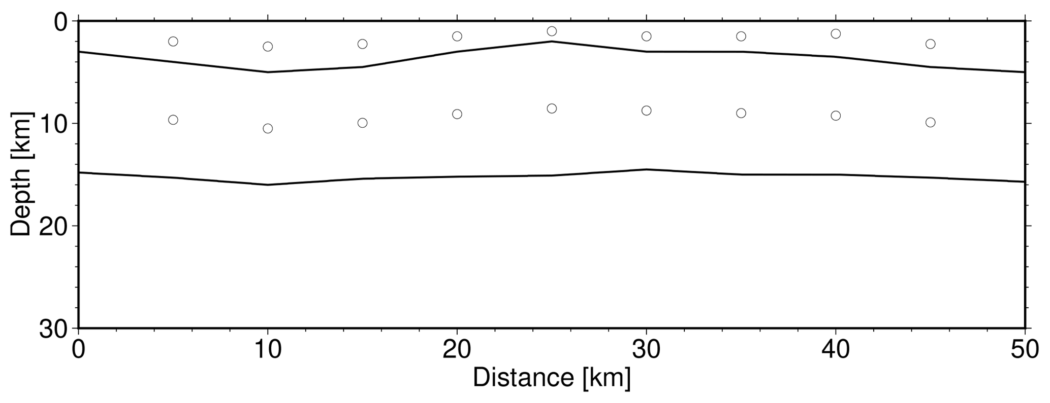
Figure 2 Simplified example of data sampling from one of the gravimetric profiles with two interpreted layers. The dots represent digitized data points used to build our model. See text for details.

The NAC model (Magrin and Rossi, 2020) had reported parameter errors for each grid point and for interfaces, so these were simply included in our data set. Seismic-refraction and wide-angle-reflection profiles (Brückl et al., 2007; Šumanovac et al., 2009) had a general estimate of velocity error of ±0.2 and ±0.1 km s⁻¹, respectively. In those cases, we simply assigned that globally estimated error to each digitized data point. In the case of the density data from the gravimetric measurements there was no error estimate. Therefore, we had to use other results in order to quantify error for that data set. Since the only other source of density data was the NAC model, and since we had no reason to believe that the gravimetric profiles we used (Šumanovac, 2010) are of a lower quality than those included in the NAC model, we assigned the maximum error estimate (to make a conservative estimate) from the NAC model to each of the points from the digitized gravimetric profiles.

The most accurate source of velocity data were refraction and wide-angle seismic-reflection profiles (Brückl et al., 2007; Šumanovac et al., 2009) and the NAC model (Magrin and Rossi, 2020), but as can be seen in Fig. 1 these studies do not cover the central and southern area of the Dinarides. Therefore, we also included velocities calculated using the values of density from gravimetric profiles (Šumanovac, 2010). In order to calculate P-wave velocities from the available densities, we used the empirical equation of Brocher (2005):

$$V_{\mathrm{P}}=\mathrm{39.128}\mathit{\rho }-\mathrm{63.064}{\mathit{\rho }}^{\mathrm{2}}+\mathrm{37.083}{\mathit{\rho }}^{\mathrm{3}}-\mathrm{9.1819}{\mathit{\rho }}^{\mathrm{4}}+\mathrm{0.8228}{\mathit{\rho }}^{\mathrm{5}},$$

where V_P is P-wave velocity in kilometers per second, and ρ is density in grams per cubic centimeter. The equation is valid for densities between 2 and 3.5 g cm⁻³ (with a correlation coefficient of ∼ 0.999), the condition which was satisfied for all the densities in the gravimetric profiles used.

The velocity in the Neogene deposits is poorly known, so it was estimated using the empirical relations of Brocher (2008) (Eqs. 1, 3, 7 and 9 in the original article). These relations account for increasing burden pressure, but not for variations in other factors. Therefore, it is justified to use these relations as a first-order approximation. We used Brocher's Plio-Quaternary relations for the shallowest parts and relations for Paleogene–Neogene sedimentary rocks for the rest of the Neogene deposits. The values obtained ranged from 0.7 km s⁻¹ for deposits close to surface to 5.6 km s⁻¹ at the greatest depth (around 7.5 km below the surface).

We used a regional EPcrust model (Molinari and Morelli, 2011) as the underlying model in order to fill the gaps in the data coverage. The EPcrust model is represented by three layers – sedimentary cover, upper crust and lower crust – with a horizontal resolution of 0.5^∘ × 0.5^∘. Each layer is characterized by laterally varying P- and S-wave velocity and density, and all of the parameters are constant for each grid point. We include EPcrust Moho, Neogene deposit bottom depth and velocity information only in parts with no other sources of data. This was done in order to remove interpolation artifacts in transition areas between the local data described before and the underlying EPcrust model. Therefore, we implemented a condition to include EPcrust data in our data set: each grid point defined in the EPcrust model had to be distanced more than 100 km in each direction from the other data point. That way, the data from the EPcrust model will not have too much influence on more relevant, local data.

For topography the SRTM15 + V2.0 model (Tozer et al., 2019) was used. It is an updated global elevation grid at a spatial sampling of 15 arcsec, and it also includes bathymetry. Since the grid of the SRTM15 + V2.0 model is much more refined than the grid we used for the definition of the model (15 arcsec in the topography model compared to about 3 arcmin in our model), a regridding has been performed by averaging all the values that fall inside one model cell.

After collecting and preparing the data, the next step was interpolation. Ordinary kriging was used to interpolate model interfaces and universal kriging when interpolating the layer properties (V_P velocity, density), as the layer properties are linearly dependent on depth (for details please see Appendix C). After interpolation, we filtered Moho interface and layer properties with a 100 km wide Gaussian filter to smooth the transitions between different data sources. The smoothing in the case of the Neogene deposits and CRC interfaces was omitted because the data used came from similar sources, and smoothing would conceal structures with relatively small spatial dimensions (e.g., Sava and Drava depressions).

Finally, we observed how the smoothing influences crustal velocity, particularly in the area covered only by gravimetric profiles. Given that the gravimetric profiles are interpreted in terms of homogeneous sections and given that the smaller sections interpreted were roughly about 100 km in dimension along the profile, we chose this as the Gaussian width. It was also confirmed by trial and error that below this width we would observe some artifacts in the model. Model uncertainty was estimated as the sum of two components: uncertainty in the input data and uncertainty from the interpolation.

4 Results

Since the model is mostly concentrated on the Dinarides, where the topmost cover is predominantly made of Paleozoic–Eocene CRC, Neogene sedimentary cover is negligible for a large part of the model, but areas to the east and northeast of the Dinarides (i.e., SW Pannonian Basin) have thick Neogene deposits reaching thicknesses of more than 4 km. Here, the most prominent features, clearly seen as two red bands in Fig. 3a, are the Sava and Drava depressions, with the Drava depression being slightly deeper.

The CRC bottom depth model (Fig. 3c) is almost a reverse image of the Neogene deposit bottom model. In the SW Pannonian Basin, where Neogene deposits are the thickest, the underlying carbonate layer is thin, and vice versa: in the Dinarides, where the CRC is the thickest, there are no prominent Neogene deposits. CRC thickness is well over 5 km in the northern part of the External Dinarides, thickening southwards and reaching cumulative thicknesses of almost 15 km in the southern Dinarides. In the Adriatic Sea area, carbonates thin out towards the southwest, but this may be partly caused by lack of available data in that part of the model.

The greatest Moho depths in the investigated region are found in the SE part of the Dinarides, reaching depths of over 45 km (see Fig. 3e). To the NW, along the External Dinarides, the Moho becomes shallower, reaching depths of around 40 km. In the SW part of the Pannonian Basin, the crustal thickness is between 20 and 30 km, becoming even shallower going further east. In the Adriatic Sea (within the part covered with our model), the Moho is shallower than in the Dinarides, but deeper than in the SW Pannonian Basin, with crustal thicknesses between 30 and 35 km. At the transition between the Adriatic Sea and the Dinarides, the Moho depth change is gradual, whereas going towards the SW Pannonian Basin from the Dinarides, the change is rather abrupt.

Given that a significant contribution to the uncertainty value is from the interpolation itself (which is of greater value at grid points further away from the input data points), one can distinctly see the areas with less data coverage as areas with higher uncertainty. Moho depth uncertainty (Fig. 3f) is low in the entire area of interest, i.e., the wider Dinarides region. For the Neogene deposit bottom, the area of lower data coverage is in the eastern part of the Internal Dinarides, where there is less information available on sedimentary thickness (Fig. 3b but see also Fig. 1). On the other hand, that part of the Internal Dinarides is mostly covered by the exposed bedrock largely composed of low-grade metamorphic Paleozoic–Mesozoic formations with a thin cover of Mesozoic CRC (e.g., Schmid et al., 2008), so Neogene deposit thickness values here are mostly negligible. For the CRC thickness, the area of least accuracy is in the NE part of the investigated area (junction zone between Dinarides–Pannonian Basin, southern Alps). Similar to the previous case, here the low accuracy is due to the lack of measurements on CRC thickness as the region is covered by a thick layer of Neogene deposits.

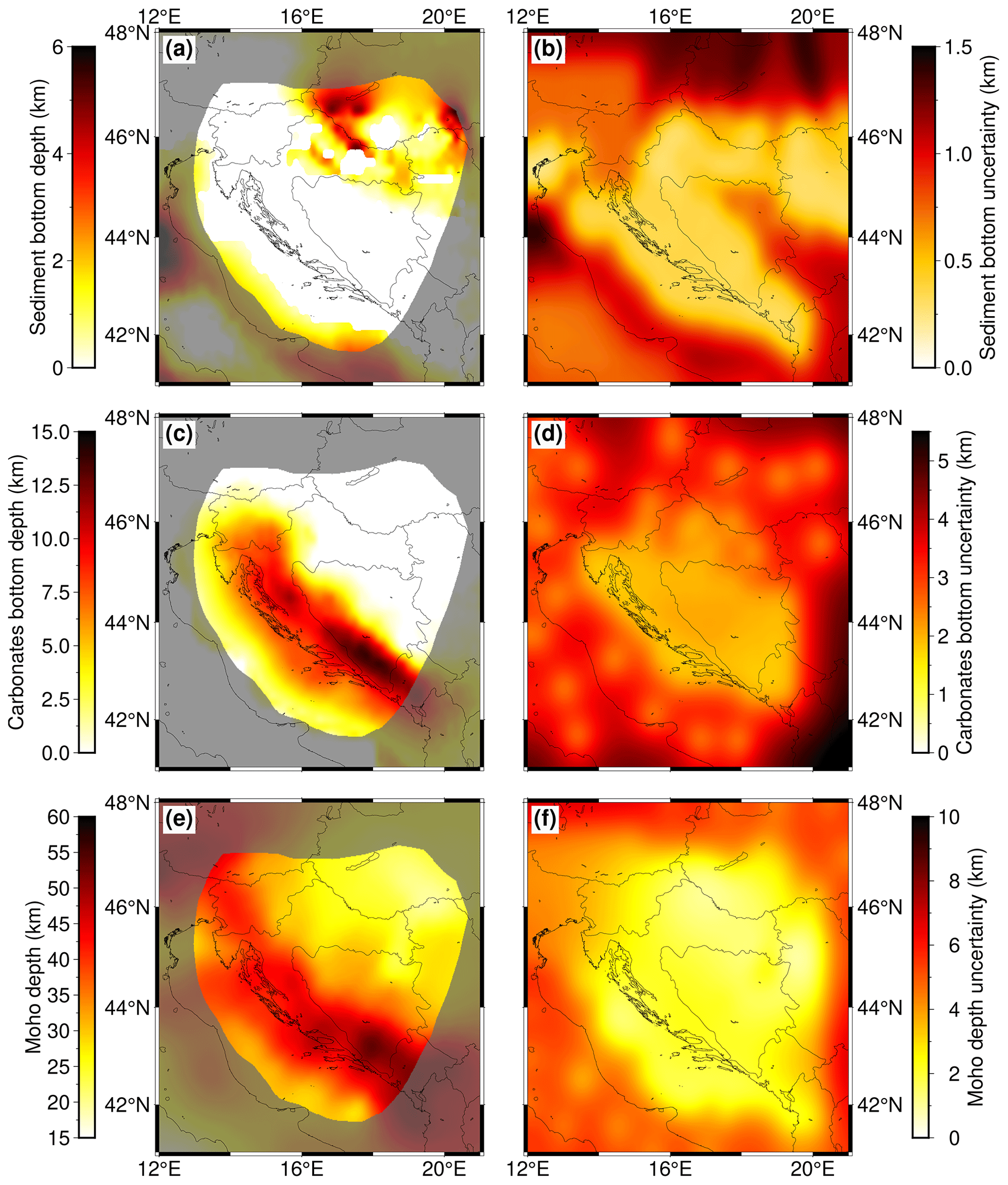
Figure 3 Model interface depths and corresponding uncertainties: (a) Neogene deposit bottom depth, (b) Neogene deposit bottom uncertainty, (c) CRC bottom depth, (d) CRC bottom uncertainty, (e) Moho discontinuity depth and (f) Moho depth uncertainty. Depths are defined as kilometers below sea level, and the areas of lower resolution are shaded.

The seismic velocity distribution within the model is depicted on the left-hand side of Fig. 4 at four depths (5, 10, 20 and 30 km), showing the most prominent features of the model crustal structure. At a depth of 5 km (Fig. 4a), the P-wave velocity in a large part of the External Dinarides is about 6 km s⁻¹. Given that we had no independent estimate for the velocity for the CRC, we cannot discern it as a separate layer just looking at velocity values. Outside the External Dinarides, one can see that the velocity in the SW Pannonian Basin at a depth of 5 km is slightly lower (just below 6 km s⁻¹) than in the rest of the investigated area.

At a depth of 10 km (Fig. 4c) the velocity values in the SW Pannonian Basin are considerably lower than in the rest of the model, with values around 6 km s⁻¹. In the area of the Internal Dinarides, velocity at 10 km depth is slightly higher than in the External Dinarides and beneath the Adriatic Sea. It is hard to discern if this reflects the actual structure or if it is the consequence of the higher uncertainty in that part of the model (the velocity here was estimated from the density values from the gravimetric profiles, given that there were no other data sources available). A similar situation can be seen in Fig. 4e for a depth of 20 km. For this depth the velocities in the SW Pannonian Basin reach values above 6 km s⁻¹, whereas values for the Dinarides are again higher (especially in the internal part) than in the rest of the investigated area, with values above 6.5 km s⁻¹. In the lower part of the crust (Fig. 4g), at a depth of 30 km, in the central part of the Dinarides the P-velocity values reach 7 km s⁻¹.

In the same image the mantle velocity values are shown in grayscale due to the considerable difference between crust and mantle values and the fact that the crustal thickness in the SW Pannonian Basin is mostly less than 25 km. The mantle velocity variations are better seen in profile sections (e.g., Fig. 5f). At the 30 km depth level, the velocity is much higher in the southern External Dinarides and below the Adriatic Sea (at least the part covered with our model) than in the northern External Dinarides.

Figure 4 also shows error estimates for P-wave velocity. It can be seen that the lowest estimates are in the area where we used the NAC model input data (Magrin and Rossi, 2020) and in areas where data from active seismic profiles were available (Brückl et al., 2007; Šumanovac et al., 2009). The distribution of the errors shown in Fig. 4 was expected given the fact that the digital NAC model and the active seismic profiles are of the highest quality and that gravimetric data have higher uncertainty. Estimated uncertainty is highest in the area where gravimetric profiles (Šumanovac, 2010) are the main source of the data used to infer P velocity.

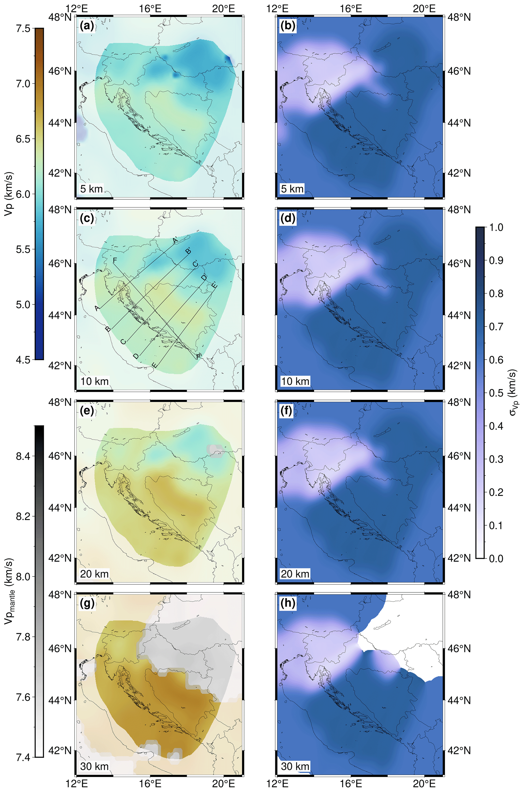
Figure 4 Velocity model depth slices and corresponding uncertainties for 5, 10, 20 and 30 km depth (below sea level) are shown in (a)–(b), (c)–(d), (e)–(f) and (g)–(h). In (c) the positions of the profiles shown in Fig. 5 are marked. The areas of lower resolution are shaded, and the gray color scale corresponds to the mantle velocity (see text for details).

Figure 5 shows depth variations in velocity along five profiles crossing the Dinarides perpendicularly and one profile (FF)^′ running parallel to the main strike of the mountain chain (locations marked in Fig. 4c). Profile AA^′ (Fig. 5a) crosses the Dinarides in their northern part. The maximum Moho depth below the Dinarides in this profile (around 40 km) is the lowest compared to the other profiles. At a distance of ∼ 270 km, the profile reaches the SW Pannonian Basin, which can be clearly seen by a thinning of the crust (between 20 and 30 km) and by the topmost layer of Neogene deposits of lower P velocity. Although the CRC thickness is indicated with the dashed line, one cannot recognize the transition into this unit by looking just at the velocity values. Generally, the velocities in the part of the profile crossing the Dinarides are larger than in the part of the profile crossing the SW Pannonian Basin. The velocity gradually increases with depth, reaching values of about 6.7–7.0 km s⁻¹ in the deepest part of the crust, with the exception of the SW Pannonian Basin, where the velocity just above Moho is lower, about 6.5 km s⁻¹.

The maximum Moho depth seen in profile BB^′ (Fig. 5b) is somewhat greater than in profile AA^′, a little over 40 km in the part of the External Dinarides. It is shallower in the Adriatic area (in the first 50 km of the profile) and in the Internal Dinarides (after about 220 km). At the very end of the profile, where it reaches the SW Pannonian Basin, one can see a similar feature as seen in profile AA^′: thinner crust and slightly lower velocity just above Moho than in the rest of the profile. In the same profile the largest CRC thickness, indicated by the dashed line, coincides with the deepest Moho and closely follows the velocity isoline of about 6.3 km s⁻¹. That feature can also be observed in other profiles (CC^′ and DD^′) at similar locations.

Profile CC^′ (Fig. 5c) crosses the Dinarides in their central part. Here the maximum Moho depth is almost 50 km. The profile reaches the SW Pannonian Basin only in the last 100 km, but it covers much of the Internal Dinarides. The CRC is of uniform thickness along the part of the profile covering the Dinarides (the first 100 km covers the Adriatic Sea area). The crust is thickest beneath the External Dinarides and becomes thinner going towards both the Adriatic Sea and the Internal Dinarides. In this central part of the External Dinarides, there is also relatively higher velocity deeper in the crust, 7.0–7.2 km s⁻¹, just above the Moho. In the Internal Dinarides (between 250 and 300 km from the start of the profile), the velocity just above the Moho is a little lower than in the external part, around 6.7–7.0 km s⁻¹. As noticed in the previous two profiles, the velocity just above Moho in the SW Pannonian Basin is even lower than in the Internal Dinarides. Similar to profile BB^′, the bottom of the CRC coincides with the velocity values of about 6.2–6.3 km s⁻¹, except in the very beginning of the profile (first ∼ 50 km).

Profiles DD^′ and EE^′ (Fig. 5d and e) cross the southernmost part of the Dinarides. Here, the Moho reaches depths of >50 km. Also, the crustal velocity at those depths is larger compared to all the other profiles, reaching almost 7.5 km s⁻¹. Variations in Moho depths and crustal velocity along the mountain chain can be best seen in profile FF^′ (Fig. 5f), running parallel to the Dinarides from northwest to southeast. In this profile, Moho depth increases from around 40 km in the northern part to >50 km in the southern part. Also, the crustal velocity just above Moho changes from just below 7.0 km s⁻¹ in the north to almost 7.5 km s⁻¹ in the south. Similarly, velocity in the mid-crustal zone (∼ 20–25 km depth) is somewhat lower in the northern part of the profile, a little over 6.5 km s⁻¹, but becomes higher in the southeastern part, reaching values of about 7 km s⁻¹.

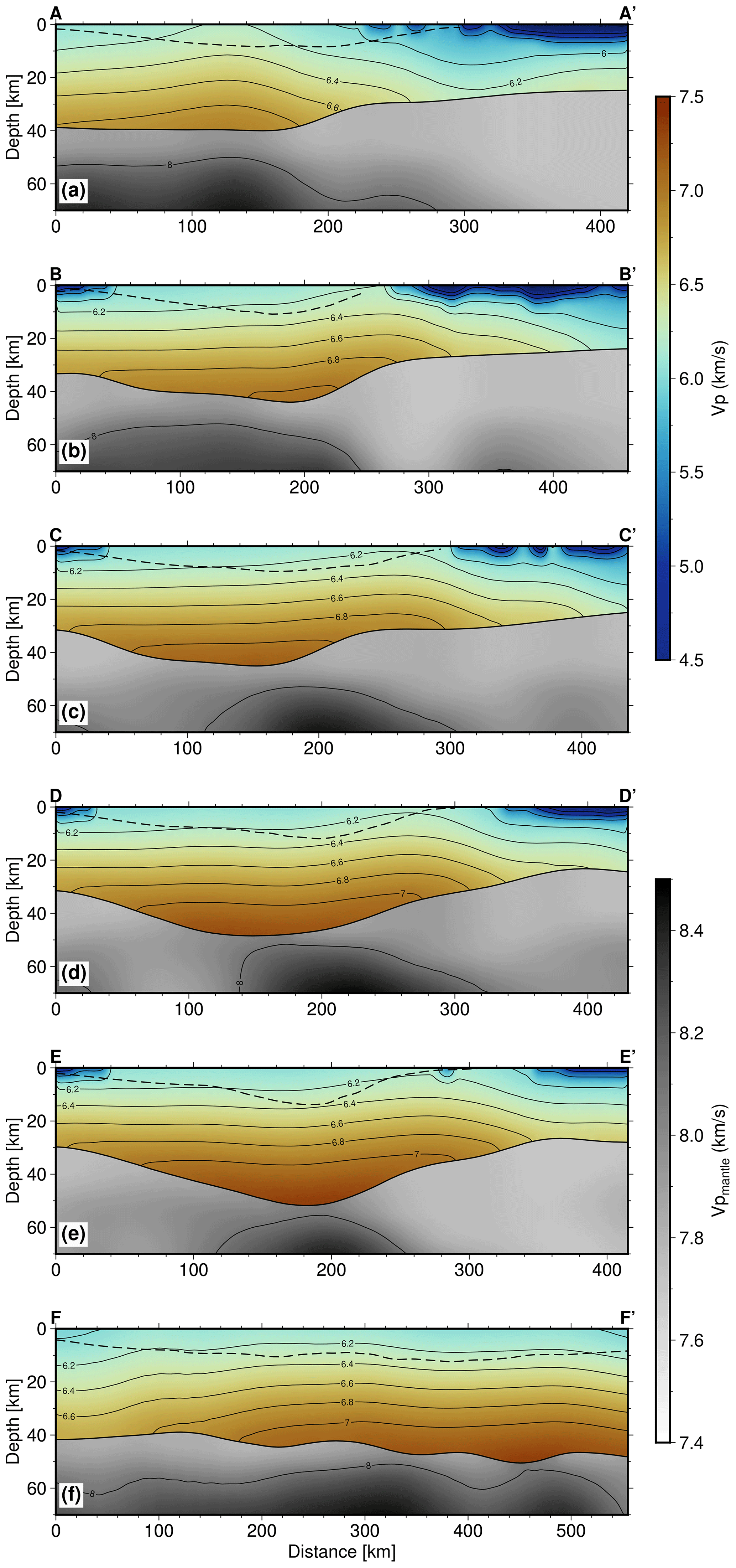
Figure 5 Profiles with locations shown in Fig. 4c: (a) AA^′, (b) BB^′, (c) CC^′, (d) DD^′, (e) EE^′ and (f) FF^′. Full parallel lines running along the profile are the velocity isolines. The depth of the CRC as derived from known geological data is indicated as the dashed line close to the surface.

From the NAC model (Magrin and Rossi, 2020) and the gravimetric profiles (Šumanovac, 2010), we have interpolated the density values for the entire crust (Fig. 6). Keep in mind that for this interpolation there were only two sources of data, one of which had densities defined as layers homogenous in density (Šumanovac, 2010). Therefore, this parameter is much less accurate than P-wave velocity. It can be seen that the density is slightly higher in the area of the Internal Dinarides than in the External Dinarides for all the depths considered here, possibly coinciding with higher-density crystalline crust. In the SW Pannonian Basin, the density has much lower values.

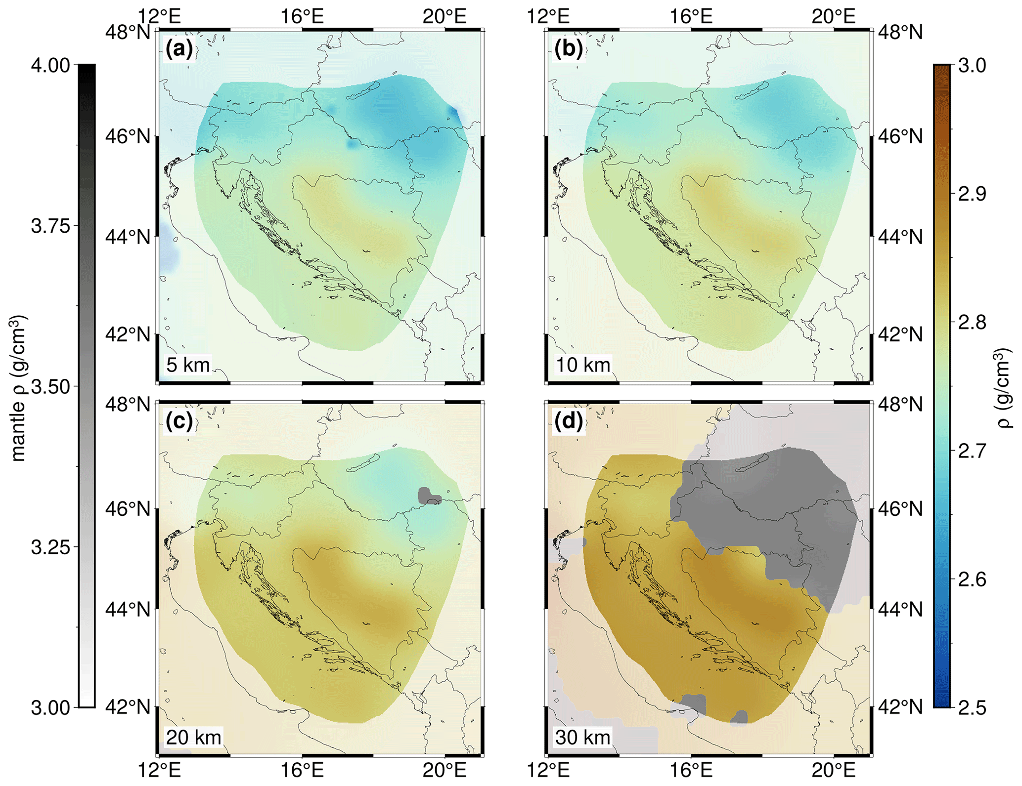
Figure 6 Density model depth slices for (a) 5 km, (b) 10 km, (c) 20 km and (d) 30 km depth. The areas of lower resolution are shaded, and the gray color scale corresponds to the mantle density (see text for details).

In the case of S-wave velocity, there were no measured velocity data (the only available V_S results were from the NAC model, which covers the western corner of our study area), so these values were estimated using the P-wave velocity and another set of empirical relations of Brocher (2005) connecting P- and S-wave velocity (Fig. 7).

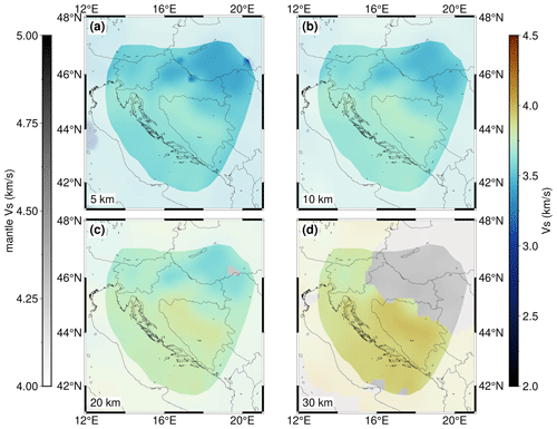
Figure 7 S-wave velocity depth slices for (a) 5 km, (b) 10 km, (c) 20 km and (d) 30 km depth. The areas of lower resolution are shaded, and the gray color scale corresponds to the mantle velocity (see text for details).

5 Model testing

To test how well the newly derived 3D model represents the true structure, we calculated the travel times for a regional earthquake recorded on representative seismic stations in the wider Dinarides area (Fig. 8). We also calculated travel times using the simple 1D model with two isotropic crust layers currently employed for routine earthquake locating in Croatia (B.C.I.S., 1972; Herak et al., 1996). The 1D model's topmost layer is characterized by P velocity of 5.8 km s⁻¹, and the deeper crustal layer has a P-wave velocity of 6.65 km s⁻¹. For the same model the uppermost mantle velocity is 8.0 km s⁻¹. We then compared the travel times from both models with the true measured travel times. We used the Pn and Pg phases of the 2020 Petrinja M_w 6.4 earthquake. The location of the earthquake (42.4188^∘ N, 16.2082^∘ E; 7.57 km) and the stations that recorded the wave onsets are shown in Fig. 8. For travel time calculation we used the fast marching method (de Kool et al., 2006) as implemented within the FMTOMO package (Rawlinson and Urvoy, 2006).

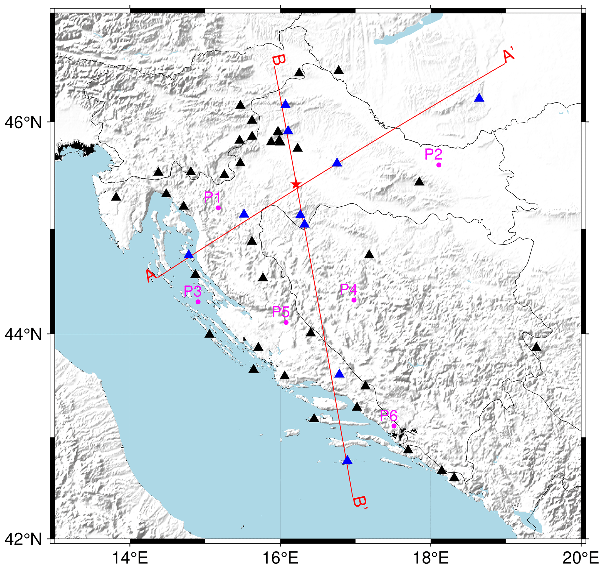
Figure 8 Epicenter of the Petrinja 2020 earthquake sequence mainshock (red star) and stations used for calculation of travel times (black and blue triangles). Travel times for all the stations are shown in Figs. 9 and 10. The red lines mark the positions of the cross-sections shown in Fig. 11 (section AA^′) and Fig. 12 (section BB^′). The stations colored blue are the ones shown in Figs. 11 and 12. The points colored in magenta mark the position of 1D models shown in Fig. 13.

Figures 9 and 10 show the differences in travel times calculated between the models (both 1D and 3D) and observed travel times for Pg and Pn phases, respectively. When looking at Pg phases (Fig. 9), we can see improvement in calculated travel time accuracy when using the 3D model (with respect to the 1D model) for epicentral distances smaller than 50 km and over 100 km. For smaller epicentral distances, the more accurate travel times in the 3D model are connected with better specification of Neogene sedimentary cover with low P-wave velocity. On the other hand, for epicentral distances between 50 and 80 km 1D and 3D model travel times are similarly offset compared to the observed travel times, with times calculated using the 1D model being slightly more accurate. We believe this is due to the less accurate velocity sampling in the upper crust in the transitional zone between the Internal Dinarides and the SW Pannonian Basin and a lack of knowledge about spatial coverage of the CRC in this area. For greater epicentral distances we can see that travel times calculated using the 3D model are much more accurate compared to those calculated using the 1D model. That means that the crustal velocity derived in our 3D model is a considerable improvement of the simple 1D model.

Concerning the Pn phases (Fig. 10), we can see that the travel times calculated using the 3D model are generally closer to the actual observed travel times for all the epicentral distances shown than those calculated using the 1D model. In the case of Pn phases, the uppermost mantle velocity plays a great part in the total travel times, so both the crustal model we derived here and the mantle model from Belinić et al. (2020) show improvement compared to the 1D model. There is still room for improvement in the uppermost mantle velocity since the model of Belinić et al. (2020) we used here is most accurate for greater depths (80–100 km).

Figure 11 shows a cross-section AA^′ (location in Fig. 8) of the newly derived 3D model, with the calculated ray paths using the simple 1D and 3D models. The position of the section was chosen in order to show travel times for both Pg and Pn phases, and we also tried to position it in such a way that it almost perpendicularly crosses the main strike of the Dinarides. There is also another cross-section shown in Fig. 12 (BB^′), oriented approximately north to south. Positions of the stations shown in cross-section BB^′ are also marked in Fig. 8. From both profiles it can be seen that the seismic rays cover completely different paths depending on whether they were calculated using the 1D or the 3D model. For example, the Pg phases, when calculated using the 3D model, travel much deeper than their 1D counterparts. Also, since the Moho in the Pannonian Basin of our 3D model is much shallower than the Moho in the simple 1D model, the calculated rays using either the 1D or 3D model travel on very different paths in the uppermost mantle. That is particularly visible in Fig. 12, in the case of the ray path between the source and the most distant station shown. The ray path calculated for the 3D model reaches depths of almost 60 km, while the same ray path calculated for the 1D model reaches depths of only 40 km. Given all that, it can be concluded that precise knowledge about the crustal model is very important for all seismic applications.

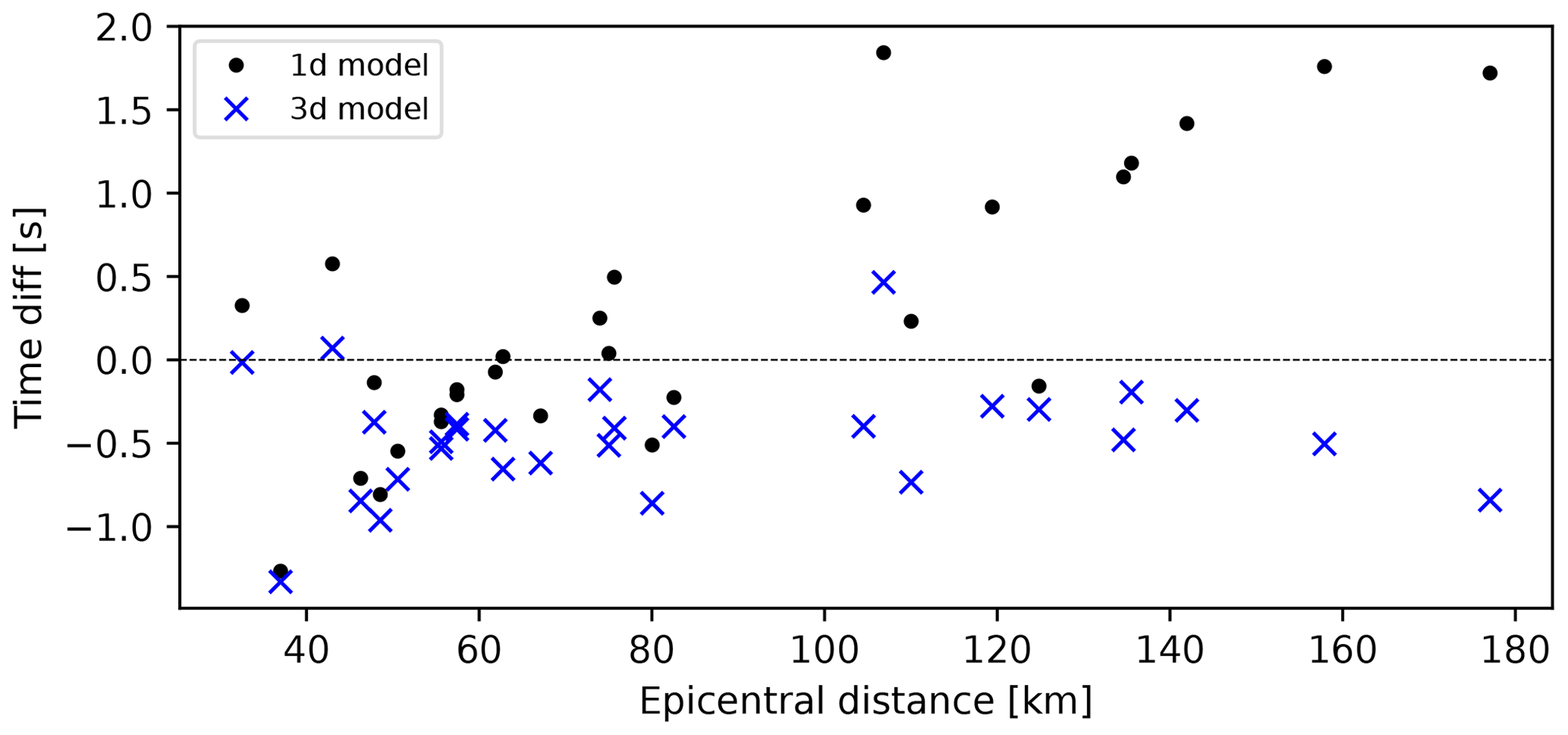
Figure 9 Pg-phase travel times for the 2020 Petrinja earthquake: time difference between 1D model and observed travel times (black dots) and between 3D model and observed travel times (blue crosses).

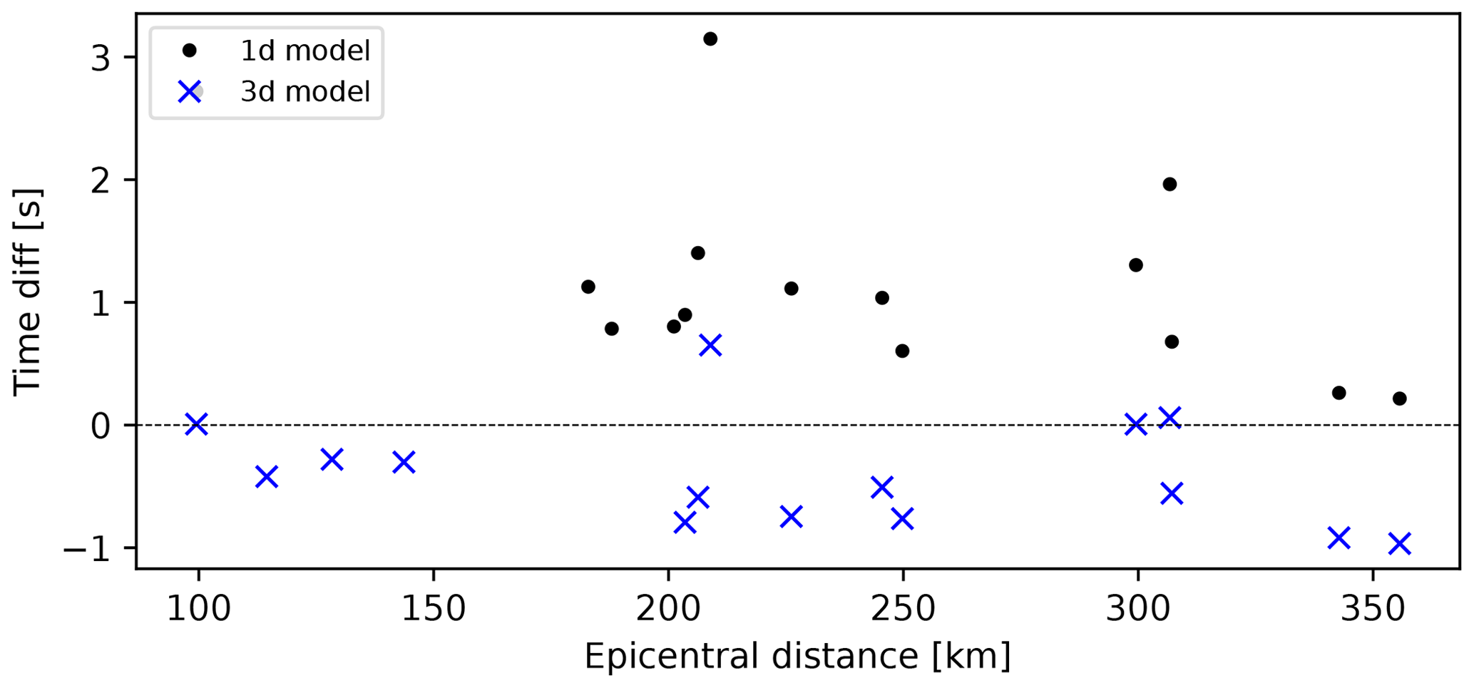
Figure 10 Pn-phase travel times for the 2020 Petrinja earthquake: time difference between 1D model and observed travel times (black dots) and between 3D model and observed travel times (blue crosses).

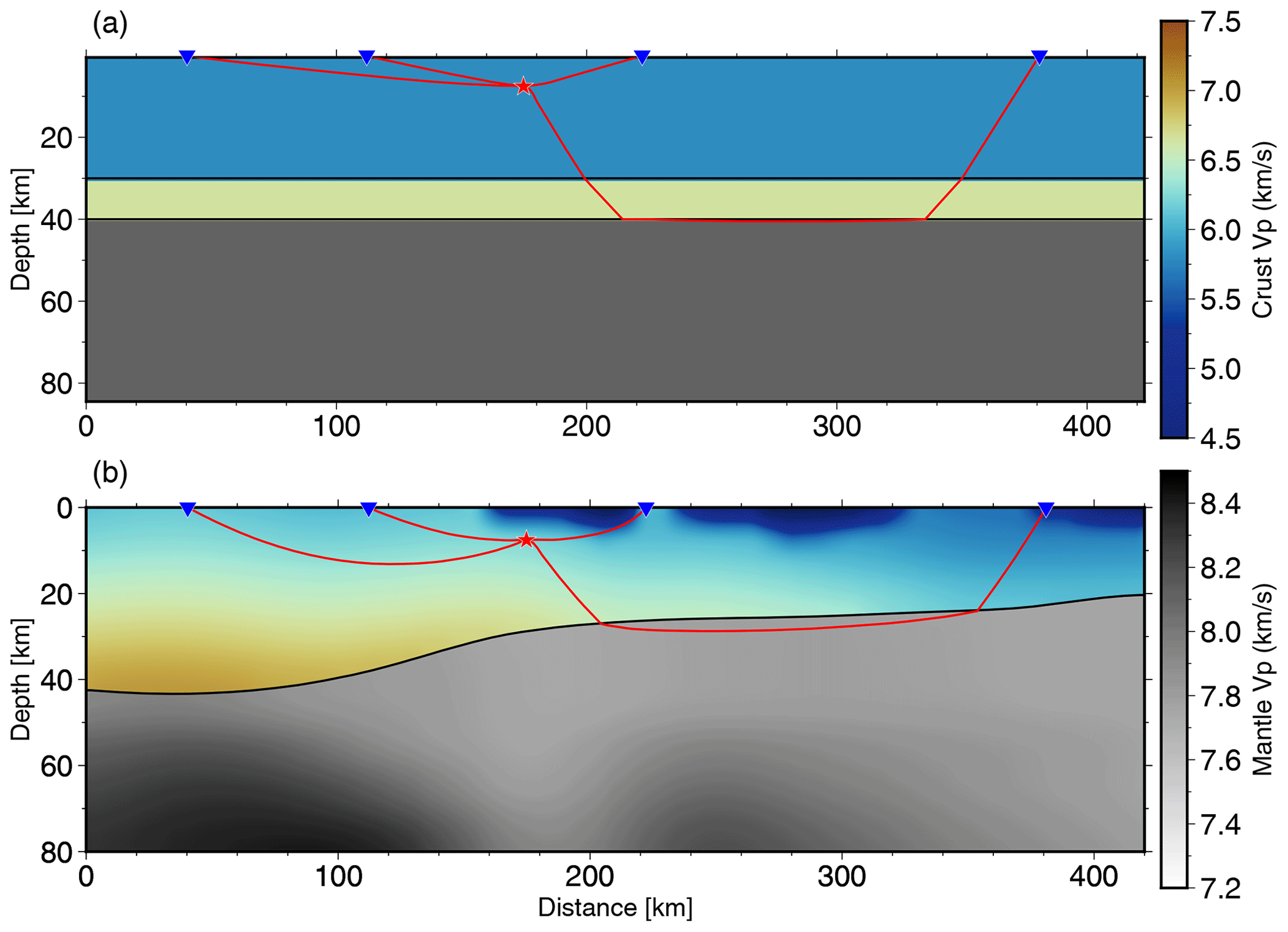
Figure 11 Earthquake ray paths in cross-section AA^′ (for location see Fig. 8) for two models: (a) a simple 1D model with two isotropic crustal layers and (b) our 3D model with one anisotropic crustal layer. Color bars are the same for both panels.

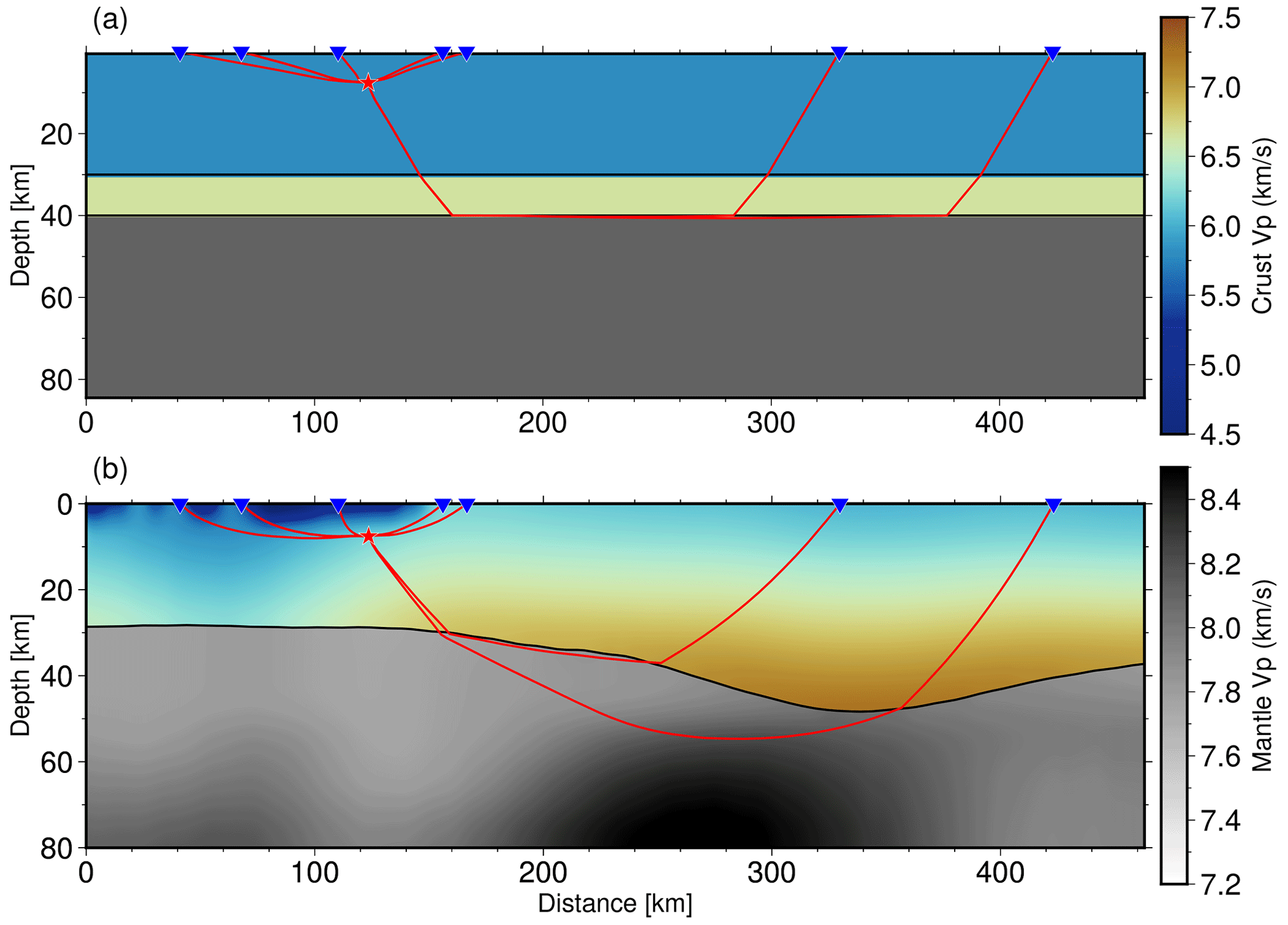
Figure 12 Earthquake ray paths in cross-section BB^′ (for location see Fig. 8) for two models: (a) a simple 1D model with two isotropic crustal layers and (b) our 3D model with one anisotropic crustal layer. Color bars are the same for both panels.

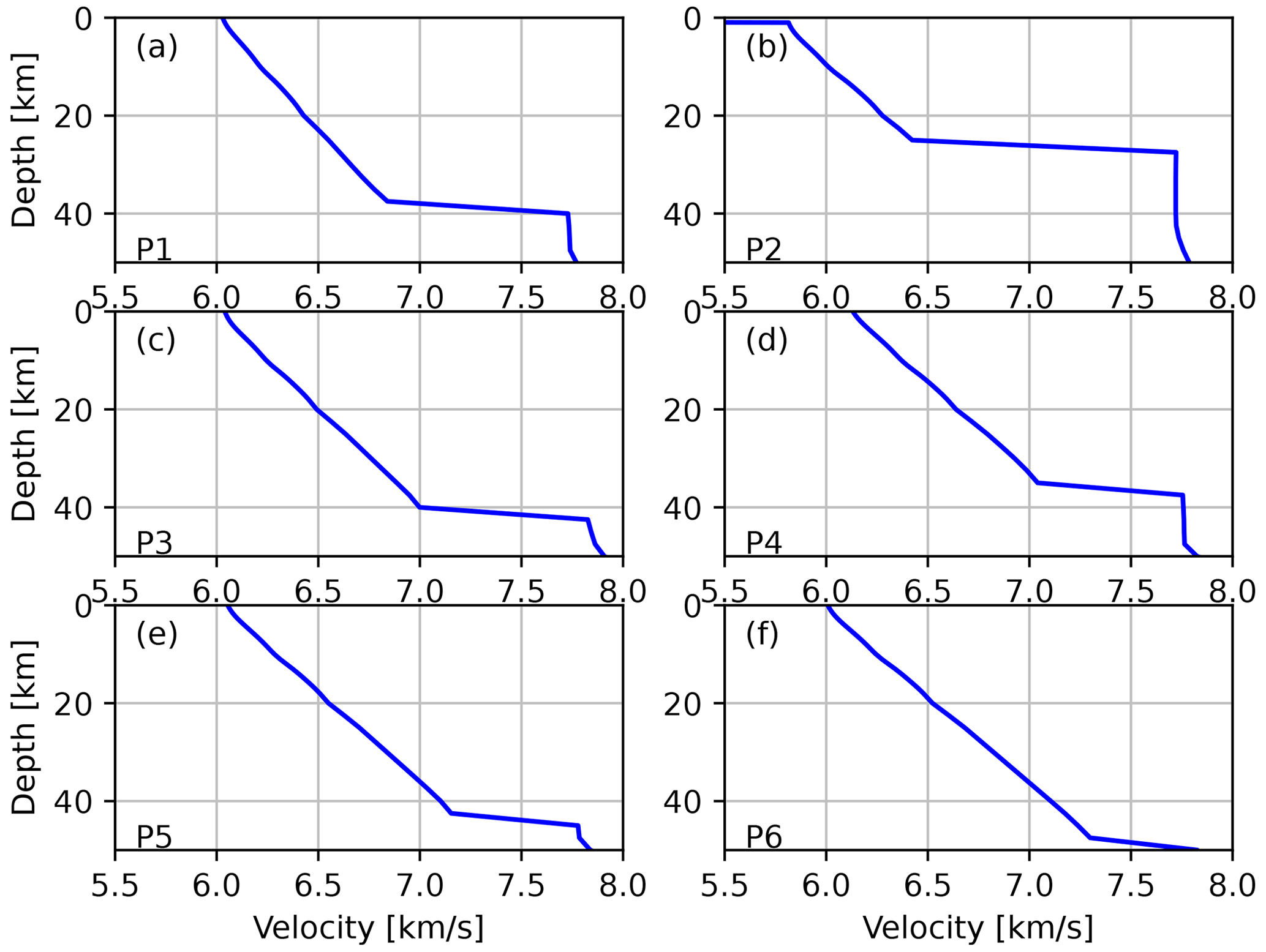
In addition to the profiles shown in Figs. 11 and 12, we also extracted depth velocity curves from the new 3D model for six points marked in Fig. 8 in magenta. Those six points have been chosen to cover different domains of our model (Stable Adria, Internal and External Dinarides, and the SW Pannonian Basin). For example, at the P2 point (see Fig. 13b), which is located in the SW Pannonian Basin, the velocity in the first couple of kilometers is much lower than for the other points because there is a Neogene deposit layer on top. The course of the curve of each model shown in Fig. 13 is generally similar at each point, with obvious differences being Moho depth (see points P2 and P1) and rate of increase in velocity with depth (e.g., compare points P3 and P5).

Figure 13 Velocity changes with depth for six points (P1 to P6; for locations see Fig. 8).

6 Discussion

The creation of the presented model was motivated by the need for a more complete 3D seismic model of the Dinarides. Although there have been previous studies estimating various properties of the crust in the region, a seismic model of the Dinarides crust and upper mantle did not exist until this study. In this work we assembled data from previous investigations to create a first comprehensive model of the crust for the wider Dinarides area. The Moho depth is the best constrained parameter of this model, since there were several good sources of high-quality data regarding this parameter. It confirms what we already know about the Moho in the Dinarides, but now it is presented as a comprehensive, ready-to-use model.

For the Neogene deposit thickness, we used manually digitized maps, therefore having less precise data but which were originally created from a high number of active seismic profiles, thus strengthening our confidence that this parameter was adequately presented in our model. The thickest Neogene sedimentary cover can be found in the area of the Sava and Drava depressions, with thinner cover in the rest of the SW Pannonian Basin and almost non-existent cover in other regions, most notably in the Dinarides, as well as in some hilly areas of the SW Pannonian Basin.

As can be seen in Fig. 1, all the high-quality P-wave velocity data are concentrated in the NW part of the study area. In the southern part, we relied on the inverted gravimetric profile data (Šumanovac, 2010), which is not the ideal data source due to the high uncertainties and lower resolution. Nevertheless, given the lack of other data sources for the southern Dinarides, even the data from the gravimetric profiles proved to be of high value. It seems that the velocity in the Internal Dinarides, where we only had inverted gravimetric profile data available, is slightly higher than in the rest of the model. At this point, we cannot discern if it is an actual feature or some artifact due to lower-quality data. The fact is that this is a separate structural unit originating from different tectonic processes, so it is not impossible that it has different features and lithological properties. If these data were omitted from the interpolation, we would have even worse results because in that case the values would be purely extrapolated. The approach we chose gave at least some constraint to the velocity values in this part of the model.

It is interesting to note that the trend of velocity in the lower part of the crust corresponds to the velocity trends in the uppermost mantle. There is a positive velocity anomaly in the part of the uppermost mantle right below (or slightly offset from) the part of the crust with the deepest Moho. These positive anomalies in the work of Belinić et al. (2020) have been interpreted as a signal of the subducting Adria Microplate. Our model is mere interpolation of what was already known, but perhaps what we see here is part of the Adria crust being dragged along with the uppermost part of the mantle in the subduction below the Dinarides. As can be seen in the profile shown in Fig. 5a, in the SW Pannonian Basin, the crustal velocity is much lower than in the Dinarides, a feature also observed by Šumanovac et al. (2009). Perhaps the lower velocity is a feature of the Pannonian crust, whereas the relatively higher crustal velocity is a feature of the Adria crust. To make a definitive conclusion, more investigation should be performed.

The velocity estimation for the Neogene deposits and the Mesozoic carbonates proved particularly challenging since there are few available data about this parameter. In the case of Neogene deposits, we used the relation of Brocher (2008) for the deposits of similar age. For the CRC we could not derive any velocity–depth relation due to the lack of available data, so in this case, we simply used the same velocity interpolation as for the rest of the crust. It seems, though, that at least in some parts of our new model, the CRC bottom depth coincides with the velocity of around 6.2–6.3 km s⁻¹.

7 Conclusions

Having a 3D model of the crustal structure is a major step forward in the study of the Dinarides and the surrounding areas. The newly derived model is defined on a regular grid for three key parameters (P and S velocity and density) and as such can be readily used by seismologists who need information on crustal structure as input for their studies (earthquake locating, seismic tomography, shaking estimation, seismic hazard etc.). We tested the performance of the model in comparison with the commonly used 1D model and found significant improvements in time travel calculations. The model still has some inherent weaknesses that have been discussed in the previous sections which are mostly connected with the limited existence of measurements in some parts of the region. Nevertheless, the 3D model represents a good first step towards improving the knowledge of the crustal structure in the complex area of the Dinarides.

The model clearly delimits several key areas (Dinarides, Pannonian Basin and Adriatic Sea) as well as distinguishes distinct layers in those regions (i.e., Neogene deposits and CRC). The most robust feature of the model is the depth to Mohorovičić discontinuity, but other parameters are also reasonably well defined. Inclusion of the CRC thickness is, to the best of our knowledge, the first attempt to estimate this parameter for the whole Dinarides region. One of the new insights found during the creation of the model is the relatively high (P-wave) velocity for the lower crust in the southern part of the Dinarides. This feature needs to be confirmed by other studies, given the sparsity of information about velocity for that region. On the other hand, the high-velocity feature fits nicely to the higher velocity of the uppermost mantle found in the same area, thus corroborating the idea of continental subduction (and/or lithospheric delamination) in the southern–central External Dinarides.

In conclusion, the model presented here represents the currently best and most complete crustal model for the wider Dinarides region. The model is assembled from all the available measurements on seismic velocity, density, layer composition and thickness to provide a full representation of the major variations in seismic wave speeds in the regional crust. Hopefully, the new 3D model will help discover some new, previously unknown features of the crust, and in turn, each new study that sheds some light on the crustal structure in this area may improve the 3D model derived here.

Appendix A

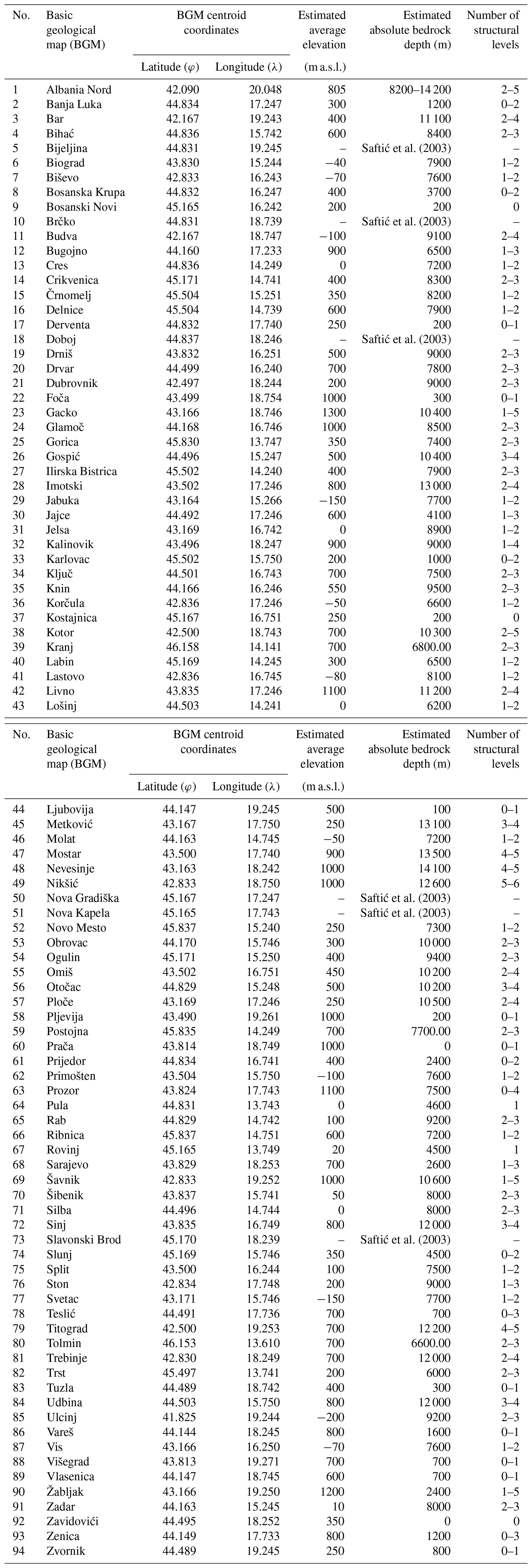
Table A1 Estimation of carbonate rock complex (CRC) bottom depth in Dinarides. CRC bottom depths were estimated based on 93 sheets of the basic geological map (1 : 100 000) of former Yugoslavia (Osnovna Geološka Karta SFRJ, 1989) and 1 : 200 000 geological map of Albania (Geological Map of Albania, 2002). The CRC bottom depth values were estimated for each map centroid with respect to External Dinarides structural relations and deformation styles that incorporate thrusting, folding (e.g., Balling et al., 2021) and thicknesses of deposits on individual maps. Regional nappe systems in the External Dinarides incorporate up to six individual structural levels composed of thrust sheets of laterally and/or vertically variable thicknesses, enabling estimated combined absolute CRC depth up to 14 200 m.

Appendix B: Input data point locations

The following figure shows the exact location of data points used for interpolation of model interfaces and parameters. Data points used for each interface and parameter are shown in a separate figure panel.

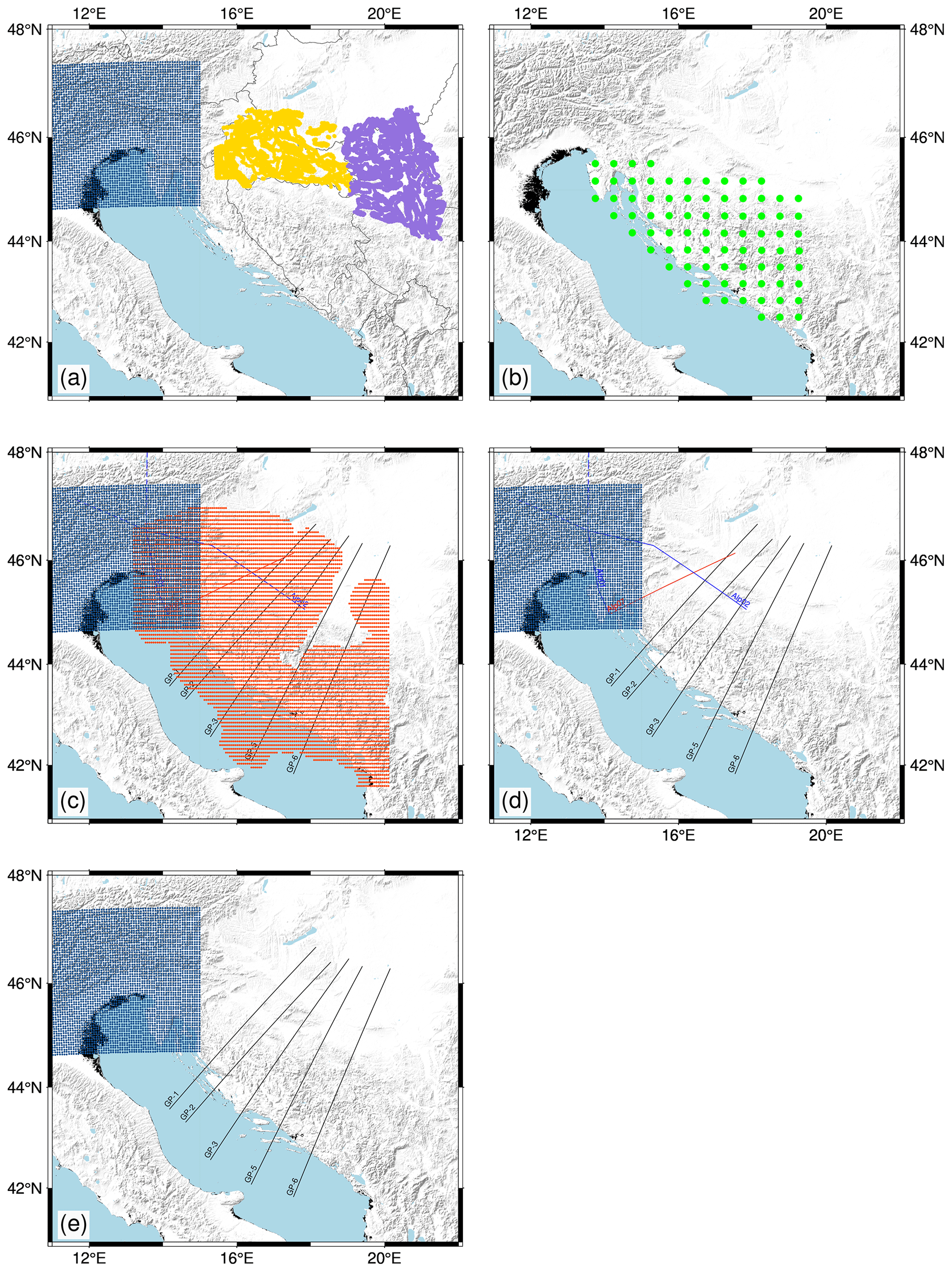
Figure B1 Point locations of data used for interpolation of (a) sediment bottom depth, (b) CRC depth, (c) Moho depth, (d) P-wave velocity and (e) density. Yellow points mark data from Saftić et al. (2003), purple points mark data from Matenco and Radivojević (2012), green points mark data on CRC depths, blue points mark data from the NAC model (Magrin and Rossi, 2020), orange points mark data from Stipčević et al. (2011), blue lines mark the positions of profiles from Brückl et al. (2007), red lines mark the profile from Šumanovac et al. (2009), and black lines mark the gravimetric profiles from Šumanovac (2010).

Appendix C: Kriging

Kriging is a method of interpolation formulated for the estimation of a continuous spatial attribute (e.g., depth to Moho interface) at an unknown site using a limited set of data from sampled sites. It is a form of generalized linear regression used for the formulation of an optimal estimator in a minimum mean square error sense (Olea, 1999).

Generally, the value at a point of interest is calculated as follows:

$$\widehat{Z}\left(x_{\mathrm{0}}\right)=\sum _{i=\mathrm{1}}^n{\mathit{\lambda }}_{i}Z\left(x_i\right),$$

where $\widehat{Z}\left(x_{\mathrm{0}}\right)$ is value estimation at the point of interest, x₀ and λ_i are weights, and Z(x_i) represents known values at site x_i. The kriging weights are derived from the covariance of the sampled values. The first step in kriging interpolation is estimation of the variogram (also called a semivariogram) – a statistic that assesses the average decrease in similarity between two random variables as the distance between them increases. It is the inverse of covariance; the covariance measures similarity, and the variogram measures dissimilarity. Unlike the other moments (e.g., the mean), the variogram is not a single number, but a continuous function of a variable h, called the lag. The variogram calculated from the sampled points is called the experimental variogram. The experimental variogram is not used in the calculation of kriging weights but is used to fit a theoretical variogram, which in turn is used for calculation of the weights. When fitting, we can use limited types of semivariograms which have acceptable properties needed for solving the system of equations in order to obtain the weights. If we would use the experimental variogram directly, we might end up with an unsolvable system of equations. For example, Fig. A1 shows an experimental and theoretical variogram used for interpolation of Moho interface depth. A variogram, such as the one in Fig. A1, that increases in dissimilarity with distance over short lags and then levels off is called a transitive variogram. The lag at which it reaches a constant value is called the range, and that constant value is called the sill. For the Moho depth interpolation, we had an abundance of data available, and we were able to estimate a theoretical variogram which fits the observed data almost perfectly.

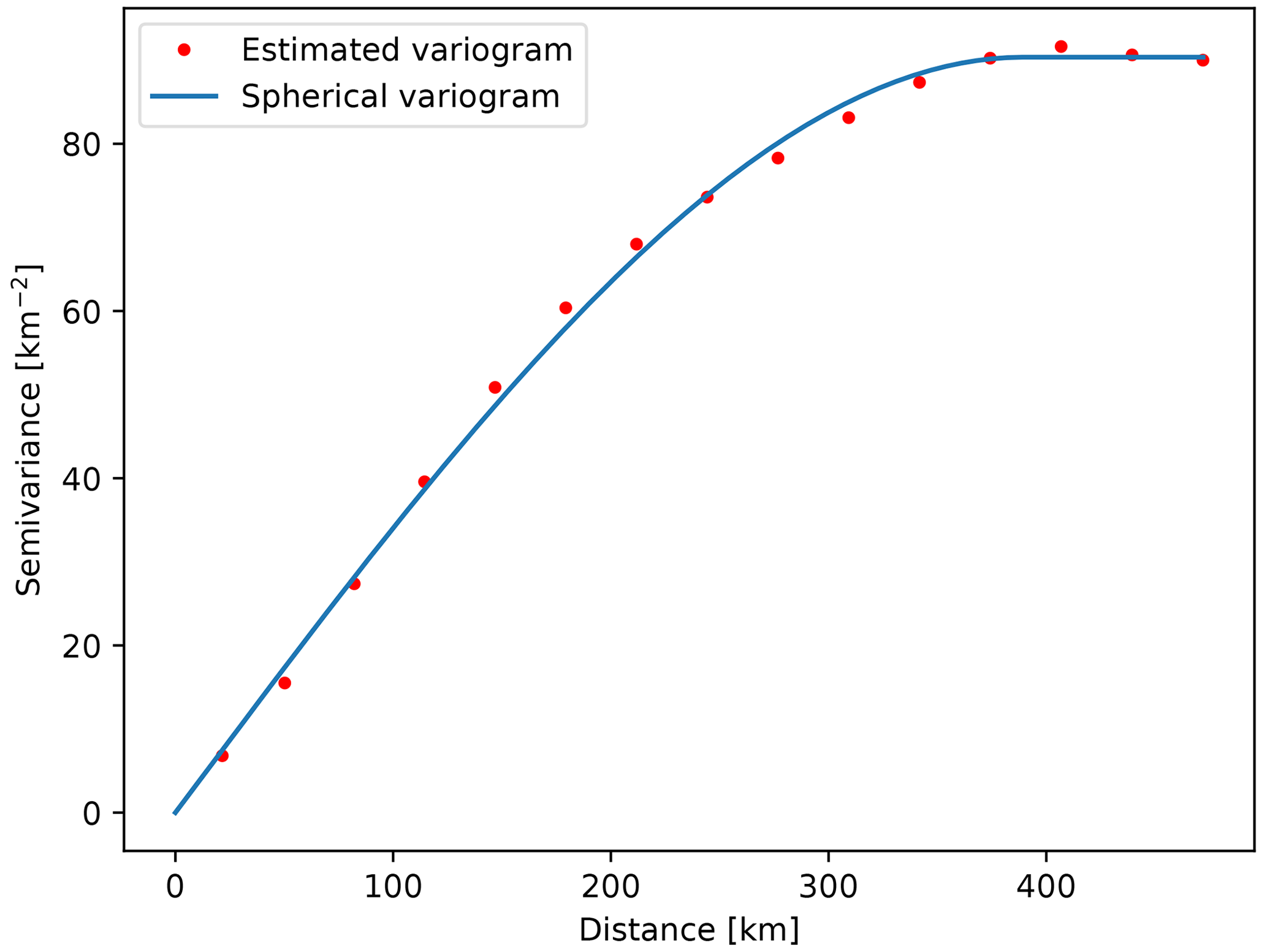
Figure C1 Estimated and theoretical (spherical) variogram used for interpolation of Moho interface depth.

In the case of other model parameters, we did not have such a perfect fit for larger lags. For instance, Fig. C2 shows the variogram used for Neogene deposit bottom interpolation. In this case, the theoretical variogram was not spherical, but exponential. In this case, for the largest lags shown, the theoretical and estimated variograms do not fit. For the calculation of the variogram pairs of measured values are used. Since for greater distances (greater lags) there are fewer numbers of such pairs, the estimates are less accurate for those lags. Fortunately, for practical use in kriging, the variogram closer to the origin requires the most accurate estimation (Olea, 1999), and we had that condition met for all our model parameters.

Figure C2 Neogene deposit bottom estimated and theoretical (exponential) variograms.

Variograms for CRC bottom depth and velocity estimation are shown in Figs. C3 and C4, respectively. The crust velocity variogram shown in Fig. C4 is required to have a constant mean in the sample space in order to be able to estimate a variogram. In the case of a gentle and systematic variation in the mean (called the drift; e.g., velocity increases with depth), it has to be removed prior to the estimation of the variogram. Such a drift was indeed observed and was removed prior to the estimation of the variogram shown in Fig. C4. Besides the drift, we estimated the experimental variogram in several directions, in order to check if it was dependent on the direction (i.e., if there was anisotropy), but we have not observed any anisotropy.

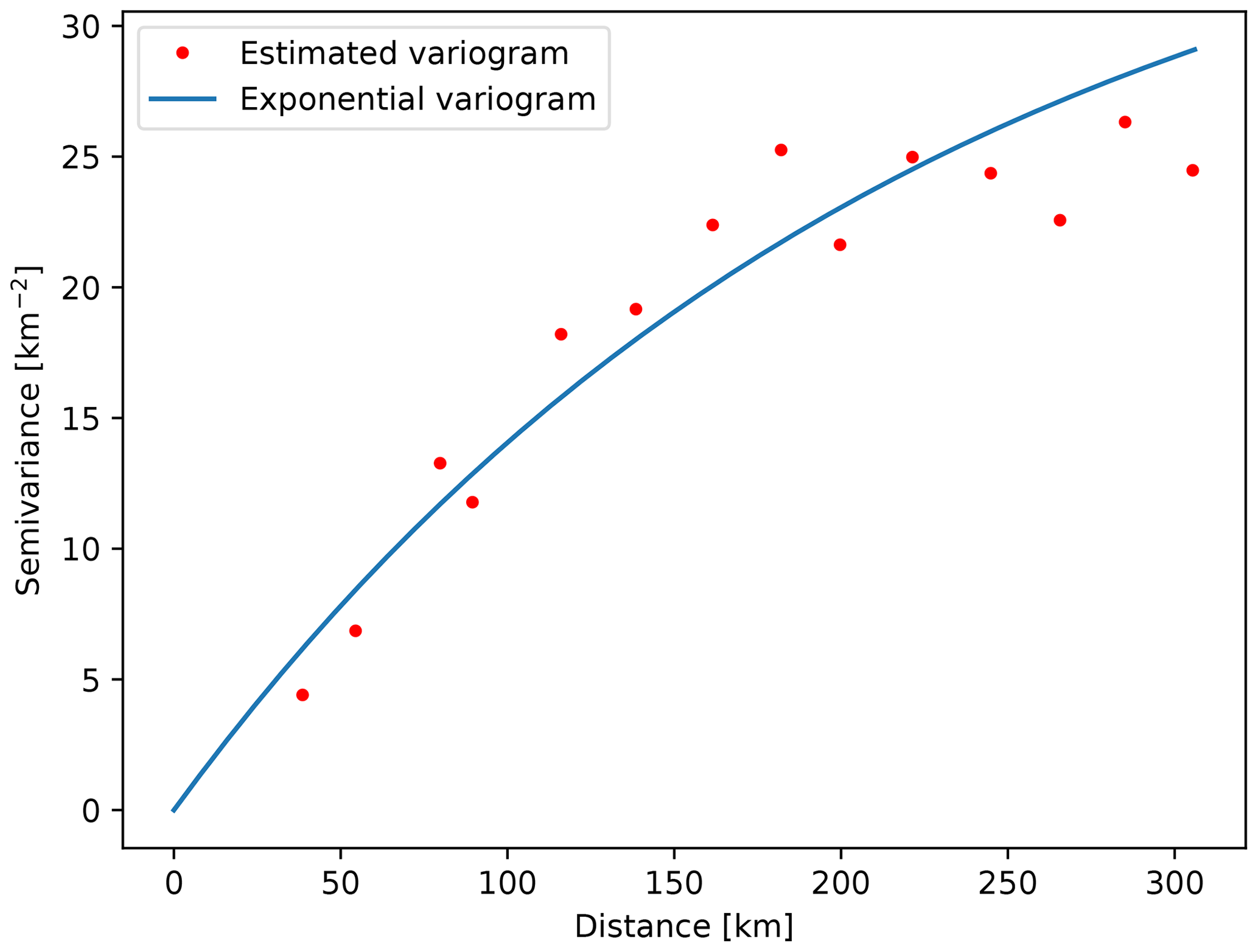
Figure C3 Carbonate rock complex (CRC) bottom estimated and theoretical (exponential) variogram.

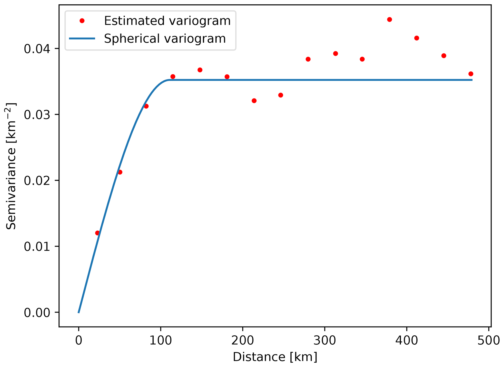
Figure C4 Estimated and theoretical (spherical) variogram used for interpolation of the crustal velocity (V_P).

Once we had variograms estimated, we were able to obtain the weights and calculate the values of parameters (Moho, Neogene deposit bottom, CRC bottom, velocity) for each point in our grid. All of the operations, both variogram estimation and the interpolation itself, were done using the gstat package (Pebesma, 2004). Alongside the interpolated values, the package also returns the variance estimates for each point in the grid.

The interface parameters (Moho, Neogene deposit bottom and CRC bottom depth) were interpolated using ordinary kriging. Ordinary kriging assumes that the mean of the value is unknown, but constant. For interpolation of the velocity, we had to use a more general type of kriging – the universal kriging. It relaxes the condition on the mean; it is no longer assumed constant. The other properties of kriging are shared between both types used. They are both minimum square error estimates. The estimation is not limited to the data interval (it is possible to extrapolate, although it is less accurate). They have so-called declustering ability; the measurements that are spatially clustered have lower weights than isolated points. They are exact interpolators with zero kriging variance, meaning that if, for instance, we try to calculate the value exactly at a sampled point, kriging will return the exact value and assign zero variance to it. It can be nicely seen in Fig. 5, showing the velocity variances. Since the variance at sampled sites is zero it is possible to discern the profiles that were sampled for data. Kriging is not able to handle duplicate points; it causes the insolvable systems of equations for the kriging weights. Therefore we had to handle such points. It is also worth mentioning that the variance returned by the kriging software does not depend on variance or values of individual observations, but only on the sampling pattern. Therefore, we added the (estimated or available) data variance to the variance obtained from the kriging and called it the total variance.

Appendix D: Comparison of the new model to existing regional models

Compared to existing regional models, Moho depth is considerably greater in the new model, especially in the southern part of the Dinarides.

The EPcrust model has sediment bottom depth defined. In our model, we discern CRC bottom and Neogene sediment bottom, which is not defined separately in the (regional) EPcrust model. Therefore, we put both of them in Fig. D2.

The horizontal variations in sediment and CRC bottom depths are much more pronounced than in the regional EPcrust model.

In the EPcrust model, the velocity is defined as two layers (upper and lower crust) with a constant velocity value (for a given grid point, it does not vary with depth; it varies horizontally, though). Therefore, we have picked two depths in our model, since we defined velocity as varying in all three dimensions. Even though we do not define crust as two layers (lower or upper crust), we have picked velocity at a depth of 15 km to compare with EPcrust upper crust and velocity at a depth of 25 km to compare with EPcrust lower crust. The comparison is shown in Fig. D3.

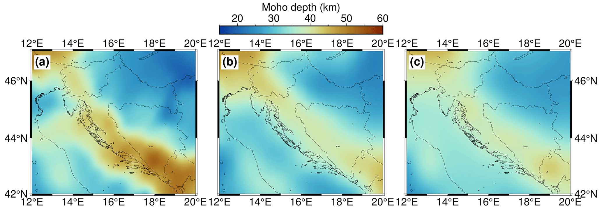
Figure D1 Comparison of Moho depths among (a) our newly derived model, (b) the Grad et al. (2009) European Moho model and (c) the EPcrust model (Molinari and Morelli, 2011).

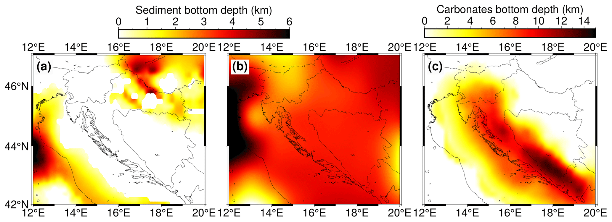
Figure D2 Comparison of sediment bottom depth as defined as (a) Neogene sediment bottom depth in our model, (b) sediment bottom in the EPcrust model and (c) CRC bottom depth in our model.

There is noticeable horizontal variation in velocity values in our model compared to the velocities defined in the EPcrust model, due to inclusion of data from refraction and gravimetric profiles.

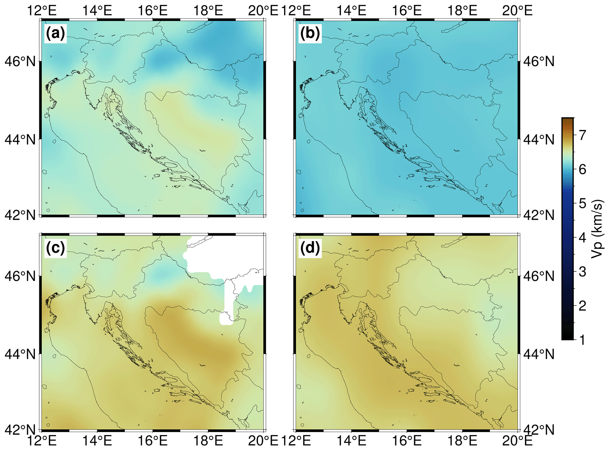
Figure D3 Comparison of P-wave velocity: (a) our model at 15 km depth, (b) EPcrust upper crust, (c) our model at 25 km depth, (d) EPcrust lower crust.