the Creative Commons Attribution 4.0 License.
the Creative Commons Attribution 4.0 License.
 | 01 Mar 2023
Ocean bottom seismometer (OBS) noise reduction from horizontal and vertical components using harmonic–percussive separation algorithms
Theresa Rein
Frank Krüger
Matthias Ohrnberger
Frank Scherbaum
Records from ocean bottom seismometers (OBSs) are highly contaminated by noise, which is much stronger compared to data from most land stations, especially on the horizontal components. As a consequence, the high energy of the oceanic noise at frequencies below 1 Hz considerably complicates the analysis of the teleseismic earthquake signals recorded by OBSs.
Previous studies suggested different approaches to remove low-frequency noises from OBS recordings but mainly focused on the vertical component. The records of horizontal components, which are crucial for the application of many methods in passive seismological analysis of body and surface waves, could not be much improved in the teleseismic frequency band. Here we introduce a noise reduction method, which is derived from the harmonic–percussive separation algorithms used in Zali et al. (2021), in order to separate long-lasting narrowband signals from broadband transients in the OBS signal. This leads to significant noise reduction of OBS records on both the vertical and horizontal components and increases the earthquake signal-to-noise ratio (SNR) without distortion of the broadband earthquake waveforms. This is demonstrated through tests with synthetic data. Both SNR and cross-correlation coefficients showed significant improvements for different realistic noise realizations. The application of denoised signals in surface wave analysis and receiver functions is discussed through tests with synthetic and real data.
- Article
(9093 KB) - Full-text XML
-
Supplement
(10224 KB) - BibTeX
- EndNote


Ocean bottom seismometer recordings are generally difficult to analyze because the noise level is usually much higher compared to land stations. At frequencies below 1 Hz, the effect of the ocean noise often dominates the data and hinders the seismological analysis (e.g., Webb et al., 1991; Crawford, 1994). Signals of interest, i.e., transient signals, especially from teleseismic events, can be masked by the oceanic noise. Here, the horizontal components are most strongly contaminated by low-frequency noise. To illustrate the noise on OBS data, we exemplary show the records of the station D10 of the DOCTAR array (see Figs. 1 and S1 in the Supplement). Various studies have tried to identify and characterize the different sources of noise recorded at the ocean bottom (e.g., Webb, 1998; Crawford and Webb, 2000; Corela, 2014; Stähler et al., 2018; Essing et al., 2021; An et al., 2021). In our study, we focus on noise sources that especially affect teleseismic horizontal recordings in the frequency band of 0.02–2 Hz. Generally, the dominant natural noise signals in the oceanic environment are secondary oceanic microseisms (Rayleigh–Scholte waves at the ocean bottom) caused by the interaction of wind-generated water waves, infragravity waves (compliance noise), and tilt noise; the latter originates from the turbulent interaction between currents and the instrument (e.g., Crawford et al., 1998; Corela, 2014). Primary oceanic microseism originates from the interaction of water waves incident at steep coastlines and/or rough seafloor (Hasselmann, 1963; Webb, 1998; Bell et al., 2015). Its spectral peak is around 0.07 Hz (Friedrich et al., 1998) in the northern Atlantic. The secondary microseism has frequencies above 0.1–0.25 Hz, with the highest spectral peak around 0.14 Hz (Friedrich et al., 1998, Fig. 1). It is caused by wind or swell waves propagating in opposite directions. The primary and secondary microseisms affect both the vertical and horizontal seismometer components, whereas the compliance noise is solely observed on the vertical component and the hydrophone. Compliance noise, which is dominant in the frequency band of 0.01–0.04 Hz, is only significant if its wavelength exceeds the water depth (Crawford et al., 1998; Crawford and Webb, 2000; Bell et al., 2015).
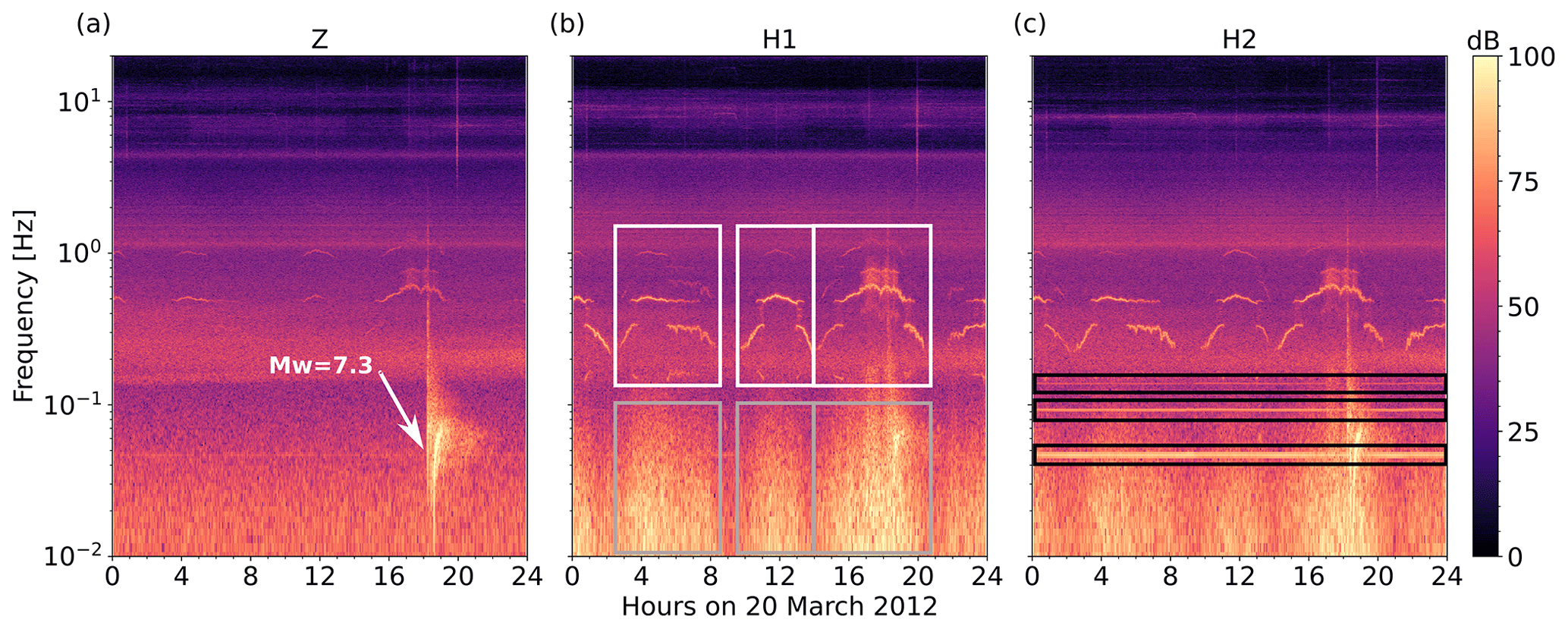
Figure 1Spectrogram of a 1 d OBS signal showing ocean bottom noise on Z (a), H1 (b), and H2 (c) components. The data were recorded by the station D10 of the DOCTAR array with a sampling frequency of 100 Hz. The spectrograms were calculated using a window length of 216 samples and an overlap of 75 %. The signal of an earthquake (Mw=7.3) on 20 March 2012 at around 18:00 at the station D10 is shown in (a). The tidal cycle of the current-induced noise is clearly visible during the high-tilt-noise episodes (gray box in b). The white box in (b) highlights the tremor episodes caused by the head buoy strumming. On H2 (c) we see instrument-related, presumably electronic noise (black boxes). The high energy of the secondary microseism band at around 0.2 Hz is visible on all components.
Below frequencies of 0.01 and 0.1 Hz, the vertical and especially the horizontal components are highly contaminated by tilt noise generated by ocean bottom currents (Webb, 1998; Crawford and Webb, 2000; Stähler et al., 2018, Fig. 1). The tilt noise level increases with signal period (see Fig. 1). The ocean bottom currents in many regions of the oceans are mostly driven by tidal force and often create a signal with the strongest amplitudes below 1 Hz, appearing every 6–12 h (e.g., Brink, 1995; Crawford and Webb, 2000; Ramakrushana Reddy et al., 2020; Essing et al., 2021). The ocean bottom currents passing the instrument create local eddy currents, deform the seafloor beneath the sensor, and tilt the whole instrument frame, to which the seismometer is fixed (e.g., Duennebier and Sutton, 1995; Webb, 1998; Romanowicz et al., 1998; Crawford and Webb, 2000; Corela, 2014; Stähler et al., 2018). Since the noise sources often act at frequencies of teleseismic earthquakes, it is crucial to improve the signal-to-noise ratio (SNR) on OBS recordings for the analysis of the Earth's crustal and mantle structure. Various studies discussed the improvement of OBS recordings through different approaches, either by suggesting a better OBS instrument design (Stähler et al., 2018; Corela, 2014; Essing et al., 2021) or by removing significant amounts of noise from the contaminated data by signal processing (Crawford and Webb, 2000; Bell et al., 2015; Janiszewski et al., 2019). Our study follows the latter approach.
Crawford and Webb (2000) developed a method to remove noise from the vertical OBS component. Calculating the linear transfer function between the horizontal and the vertical component allows estimating the tilt noise, which can then be subtracted from the vertical component. Pressure data measured in parallel to the seismometer recordings allow reducing the influence of infragravity waves on the vertical seismometer component recordings. For better results, Bell et al. (2015) propose first rotating the horizontal components in the direction of the highest coherence between the horizontal and vertical component before calculating the linear transfer functions. The mentioned methods solely improve the SNR on the vertical component, whereas the noise contamination on horizontal components is often larger. Other recent studies have also attempted to reduce noise on the horizontal components (Mousavi and Langston, 2017; Zhu et al., 2019; An et al., 2021; Negi et al., 2021). An et al. (2021) tried to reduce the noise on the horizontal components by applying the reversed procedure of Bell et al. (2015). Rotation of one horizontal component in the direction of the principle noise indeed results in an improvement of the orthogonal horizontal component, but the other horizontal component became noisier (An et al., 2021). Results of a recent study applying a polarization filter to reduce the noise on all components show strong changes in the broadband waveforms (Negi et al., 2021). The automatic noise attenuation method developed by Mousavi and Langston (2017) is a time–frequency denoising algorithm using the wavelet transform and synchrosqueezing. It can be used to keep the signal and remove the noise or vice versa. The decomposition method DeepDenoise from Zhu et al. (2019) is based on a deep neural network. DeepDenoise decomposes the waveform into signal and noise in the time–frequency domain. The latter methods both improve the SNR but mainly focus on local and regional earthquake detection. They result in changes in the waveform shape if the noise amplitude directly ahead of the signal is significant in comparison to the signal amplitude in a specific frequency. However, the analysis of undistorted broadband waveforms on the horizontal components is crucial for many passive seismological structure analysis methods, e.g., the calculation of receiver functions or surface wave dispersion and polarization analysis.
Here we introduce a method inspired from music information retrieval (MIR) research, which is adapted to seismological data and used for noise reduction on both the vertical and the horizontal components.
Seismic waveforms and acoustic signals generated by musical instruments are similar in some respects (Schlindwein et al., 1995; Johnson and Watson, 2019). The extensive research in the field of music information retrieval has resulted in advances (e.g., Müller, 2015) that may be useful in seismic signal processing as well. Exploiting the idea of harmonic–percussive separation (HPS) in MIR, Zali et al. (2021) developed an algorithm to separate harmonic volcanic tremor from earthquakes in seismic waveforms. In the present study we use this algorithm after some modifications in order to separate “harmonic” (long-lasting narrowband signals) and “percussive” (broadband transients) components of an OBS data set aiming at noise reduction and retrieval of clearer broadband earthquake waveforms. Throughout this study we will make use of the term noise for any signal other than earthquake signal in the data set. In the context of OBS noise reduction using HPS algorithms, percussive components correspond to earthquake signals and harmonic components correspond to noise signals. Long-duration OBS noise signals that last a few hours to days (depending on the noise type) with a restricted frequency range contrast with transient seismic signals such as earthquakes with a wider range of frequencies.
The algorithm introduced in Zali et al. (2021) is a combination of two HPS approaches that leads to the desired signal separation. Here we also use the two approaches in sequence in order to separate different types of noise signals from the earthquake signals. In the first step we use a similarity matrix (Rafii and Pardo, 2012; Rafii et al., 2014) to separate monochromatic and harmonic noises. In the second step we use median filtering (FitzGerald, 2012) in order to separate the remaining narrowband signals. With this two-step approach we can separate and remove much of the OBS noise contamination from the earthquake signals.
In this study, we discuss the noise recorded by a LOBSTER (Long-term OBS for Tsunami and Earthquake Research) OBS instrument from the DEPAS pool, which is equipped with a Güralp CMG-40T seismometer and an MCS (marine compact seismic) recorder (for technical specification see Stähler et al., 2018). We show data recorded during the DOCTAR deployment using DEPAS LOBSTERs located around the Gloria Fault in the northern Atlantic. A total of 12 DEPAS LOBSTERs form the array; they were deployed between 2011 and 2012 and recorded data with a sampling frequency of 100 Hz (Hannemann et al., 2016, 2017).
We observed a continuous harmonic signal at a frequency of 0.04 Hz, partially with one or two overtones on a subset of the array (see Fig. 1). This signal was observed at 30 % of the stations from the DOCTAR project (e.g., Hannemann et al., 2016, 2017) and at 43 % of the stations from the KNIPAS project (Schlindwein et al., 2018), both using the mentioned DEPAS LOBSTER design. We cannot identify the source of this signal yet, but based on its continuity, we assume an electronic source from the instrument itself.
The hydrophone and especially the horizontal components are highly affected by the strumming of the head buoy, which is attached to the DEPAS LOBSTER frame, causing a “current-induced harmonic tremor signal” (Stähler et al., 2018; Essing et al., 2021, Fig. 1). These “tremor events” last over up to 4 h and appear every 6–12 h. These presumably tidal-driven tremor events are harmonic signals with a fundamental period of 0.4–1 s and various overtones (1–10 Hz) (Stähler et al., 2018; Essing et al., 2021, Fig. 1). Regarding the frequency band, tremor events mainly affect the analysis of teleseismic body waves, especially on the horizontal component (Fig. 1).
3.1 Harmonic–percussive separation (HPS)
Harmonic–percussive separation refers to the problem of decomposing a signal into its harmonic and percussive components. This topic has received much attention in recent years (Rafii et al., 2018) and has numerous applications in the field of MIR and musical signal processing.
Within a general context harmonic signals show an overtone structure in the spectral domain. We call overtones one or more clear narrowband frequency peaks that are integer multiples of the fundamental frequency (the first frequency peak in the spectrum). Harmonic signals have relatively stable behavior over time and can be identified in a short-time Fourier transform (STFT) spectrogram by horizontal structures referring to constant frequencies along the time axis.
In contrast, percussive signals form vertical structures in an STFT spectrogram that contain energy in a wide range of frequencies. Therefore, it is a straightforward strategy in most HPS algorithms to try to separate the horizontal structure from the vertical structure in the spectrogram corresponding to harmonic and percussive components, respectively. The horizontal lines in the spectrogram could correspond to either harmonic signals or monochromatic signals.
3.2 HPS using median filtering (MED)
One of the simplest and fastest HPS approaches is median filtering (FitzGerald, 2010). For simplification we name this algorithm MED in this study. Median filters are usually used to remove noise from an image or a signal. Using a median filter a sample will be replaced by the median of neighboring samples within a window of a specific length (the specific length is the kernel size of the median filter). The entire signal is processed using a sliding window analysis. Within the HPS, two median filters are applied to the amplitude of the STFT spectrogram of a signal. One median filter is performed along the time axis of the spectrogram to suppress percussive events and enhance harmonic components. Another median filter is applied along the frequency axis in order to enhance percussive events and suppress harmonic components. The two resulting spectrograms are then subsequently used to create two masks, which are applied to the original signal spectrogram separately to generate two spectrograms of harmonic and percussive components, respectively. For creating the harmonic and percussive signals in the time domain the phase of the original signal is added to each spectrogram, and the time domain signals are reconstructed using the inverse STFT.
3.3 HPS using the similarity matrix (SIM)
Another powerful approach in HPS proposed by Rafii and Pardo (2012) is based on calculating a similarity matrix. We name this algorithm SIM here. This approach is a repetition-based separation, which identifies repeating elements in the spectrogram by looking for similarities by means of a similarity matrix. Within the SIM algorithm, first similar time frames in the spectrogram are identified through a similarity matrix. Then a median filter is applied only to the frames identified as similar to constitute the repeating spectrogram model that corresponds to harmonic components. The non-repeating spectrogram that corresponds to the percussive component of the data is obtained by subtracting the repeating spectrogram from the original spectrogram. For creating repeating and non-repeating signals in the time domain, the phase of the original signal is added to each spectrogram and the time domain signals are reconstructed using the inverse STFT. Details of this approach are discussed in the following section.
3.4 HPS noise reduction algorithm for OBS data
The motivation for using HPS for noise reduction of OBS data stems from the different characteristics of earthquake and OBS noise signals as described in Sect. 2. Earthquakes are broadband transient signals, while the signals of OBS noises are more narrowband compared to earthquakes. We combine two modified HPS algorithms to separate those signals in a two-step procedure. We divide the frequency content of the signal into two frequency ranges: the MED frequency range covers the frequency range between 0.1 and 1 Hz, whereas the SIM frequency range contains the complementary frequency range, i.e., all frequencies except the band between 0.1 and 1 Hz. Then two different algorithms are applied to these ranges. In the first step, we use the SIM algorithm and separate only harmonic or monochromatic signals from the original records in the SIM frequency range. The reason is related to the frequency content of the noise and earthquake signals and how the SIM algorithm separates them. For a better understanding, we first explain how the algorithm works and then present more detail about this selection. In the second step, to reduce noise from MED frequency range we apply MED. There we target harmonic (or monochromatic) as well as narrowband signals with gliding frequencies named current-induced harmonic tremor signal in Sect. 2. The overall schematic diagram of our HPS noise reduction algorithm along with an example is shown in Fig. 2.

Figure 2Method flowchart (a) with an illustration of the processing steps with a real data example. The left panel shows the first step of the method; using the similarity matrix (SIM) in the frequency range below 0.1 Hz and above 1 Hz, we divide the spectrogram (X) of the original signal (SO) into two spectrograms of repeating (R) and non-repeating (NR) patterns. The right panel shows the second step of the method wherein we apply a median filter (MED) to the frequency range of 0.1 to 1 Hz (spectrogram X′) in order to remove noises from this frequency range. It results in the harmonic spectrogram (H). As the interesting frequency range for OBS signals is below 1 Hz, the spectrograms show only this frequency range. Finally, the noise spectrogram (N) is created by summing the separated noises derived from two steps, and the noise signal (NS) is derived using ISTFT. We obtain the noise-reduced signal (HPS) by subtracting the NS from the input OBS signal (SO). STFT: short-time Fourier transform. HPS: harmonic–percussive separation. SIM: similarity matrix. MED: median filtering. ISTFT: inverse short-time Fourier transform. (b) Spectrum of the original signal (SO) and the HPS noise-reduced signal.
The SIM algorithm is explained in the following: from the original OBS record SO (SO represents the original restituted OBS signal) we derive the STFT named X, which is a complex-valued spectrogram.
The complex-valued spectrogram X is separated into its amplitude and phase components using Eq. (1):
where φ is the phase of X, is the amplitude of X, and j is the imaginary unit.
All of the spectrogram modifications will be applied to the amplitude spectrogram V. The cosine similarity (the similarity between two vectors of an inner product space) between the STFT time frames is calculated through the multiplication of the transposed V by V with the normalization of the V. This is shown in Eq. (2):
where S is the similarity matrix. Each point (ka,kb) in S is the cosine similarity between time frame ka and kb of , where m is the number of time frames and n is the number of frequency channels for each time frame. Once the similarity matrix is calculated we use it to determine the time frames most similar to each single time frame. For time frame ka we compare all the values in S(ka,ki) for . We identify similar frames for time frame ka by choosing the upper 2 % of the all time frames with the highest similarities.
Finally, all time frames similar to any frame k in V are stored in a temporary array K. Those similar time frames are used to create a repeating spectrogram model W. The corresponding frame in W is obtained by taking the median of K for each frequency at each time frame k. Those time–frequency bins, which are similar with little deviation between repeating frames, are captured by the median and constitute the repeating spectrogram model. This spectrogram contains only similar and repeating patterns. The time–frequency bins with large deviations between repeating frames would constitute non-repeating transient patterns and would be suppressed by median filtering.
The nonnegative spectrogram V is the sum of two nonnegative spectrograms of repeating and non-repeating patterns; hence, W (the repeating spectrogram model) should always have smaller values or at most be equal compared to V. To ensure this, a repeating spectrogram model is defined by taking the minimum between W and V. The non-repeating spectrogram model is derived by subtracting from V.
We use these two (the repeating and the non-repeating) spectrogram models to create two time–frequency masks for repeating and non-repeating patterns, respectively. Instead of the binary mask, which is used in Rafii and Pardo (2012), we use a soft mask via Wiener filtering (Vaseghi, 1996), which is more flexible and usually leads to a better result. The calculation of the soft masks is shown in the following equations:
in which M1 and M2 are repeating and non-repeating masks, respectively. We multiply the masks with the input amplitude spectrogram V to separate the repeating and non-repeating components. The element-wise multiplication of the masks by the input amplitude spectrogram V is shown in the following equations:
in which R and NR denote repeating and non-repeating amplitude spectrograms, respectively.
The resulting R and NR spectrograms are shown in Fig. 2a for a specific and/or typical example of an OBS recording. As can be observed in the R spectrogram, the low-frequency harmonic or monochromatic signals below 0.1 Hz in particular are well captured. We applied the SIM algorithm only to the frequency band below 0.1 Hz and above 1 Hz. In the frequency band from 0.1 to 1 Hz the signals remain unchanged by this procedure. This is the first constraint we consider for the SIM algorithm. In the field of noise reduction using signal processing techniques, a very important point is to not modify the signals of interest for analysis. P and S waveforms in teleseismic earthquake signals often have frequency content in the range of 0.1 to 1 Hz with a dominant frequency around 0.3 Hz. Oceanic microseism noise, which is usually present in OBS data, has a dominant frequency around 0.1 to 0.3 Hz. As P and S phases have a similar dominant frequency as the microseism noise wave field, superposition of both wave fields could happen in this frequency range. They could interfere constructively or destructively, so the resulting amplitude could be higher or lower compared to the original P- or S-phase amplitudes. Considering these interferences, using the SIM algorithm, may result in creating fake higher amplitude for these phases or losing part of their amplitude in the noise-reduced signal. But this could be problematic only when the amplitude of the noise changes over time. For a noise signal with almost constant amplitude, the SIM algorithm can extract the true amplitude of the noise even in the interference moments. However, the microseism noise has slightly varying amplitude over time.
Before moving to the second step we introduce a second constraint parameter, which we use in the SIM algorithm. Surface waves of teleseismic events usually show a dispersed narrowband signal and correspond to mainly horizontal patterns of short duration (on a daily scale) in the spectrogram. Given the way the HPS separates harmonic from transient signals, the surface wave train may be erroneously recognized as the harmonic component and thus be separated as noise signal. In order to prevent this and preserve the whole frequency content of the earthquake, we define a so-called waiting factor for the similarity calculation, introducing a minimum time distance between two consecutive similar frames. For the problem of retaining teleseismic surface waves we found that a waiting factor of at least 2 h prevents the algorithm from pruning surface waves from the transient signal part. The rationale is that the duration of a teleseismic event is usually less than 2 h, whereas the noise components have a longer duration. Using this waiting factor prevents separating any harmonic component of the earthquake signal as noise component. As a side effect this constraint causes short-duration harmonic–monochromatic noise signals to also not be well captured. However, these types of signals are not common in OBS data (see Sect. 2).
In the second step of our algorithm, to target noise signals in the frequency range of 0.1 to 1 Hz, we use MED as it is described in Sect. 3.2. We apply this second part of the noise removal procedure only to a restricted frequency band of 0.1 to 1 Hz. The dominant noise in the MED frequency range is the current-induced harmonic tremor signal (see Sect. 2).
First we create the X′ spectrogram, which is equal to X in the MED frequency range and is equal to zero outside this band. Then we apply a horizontal median filter to X′ in order to separate harmonic components. This results in the harmonic spectrogram H, which contains nearly horizontal patterns captured by the median filter.
Now we have two separated spectrograms for noise signals: R, which is derived from the first step, and H, which is derived from the second step. Summing these two spectrograms will build the noise spectrogram N. Subtracting N from the input amplitude spectrogram V will construct the transient spectrogram T.
As can be seen in Fig. 2a in step 2, the dominant energy of the narrowband signals with gliding frequencies in the range of 0.1 to 1 Hz (the current-induced harmonic tremor noise as introduced in the Sect. 2) is captured in the noise spectrogram N, but part of it remains in the transient spectrogram T. Signals with changing frequency which do not form complete horizontal lines in the spectrogram are difficult to capture by our HPS algorithm, so some of their energy remains in the final spectrogram.
3.5 Reconstruction of the denoised signal
In order to reconstruct the noise-removed signal in the time domain we must add phase information to the spectrogram. We separated the complex-valued spectrogram X into its amplitude V and its phase component using Eq. (1), and all the further modifications have been applied to the amplitude spectrogram V. The phase of input signal SO is mostly affected by the phase of noise signals as they have the dominant energy in the signal. Therefore, we use the phase information of SO in order to reconstruct the noise signal. We add this phase to the noise spectrogram N using the following equation:
where N′ is the complex-valued noise spectrogram. We reconstruct the noise signal NS from the complex spectrogram N′ using the inverse STFT. Finally, the OBS denoised signal HPS (HPS here represents the SO signal after the HPS processing) is obtained by subtracting the noise signal from the input OBS signal SO using the following equation:
3.6 Parameter selection
Many typical noise signals observed in OBS recordings are harmonic, monochromatic, or narrowband signals with gliding frequencies (see Sect. 2). In order to extract the expected narrowband noise signals from the STFT we require a high-frequency resolution in the spectral domain, therefore making it necessary to use sufficiently long time windows for the spectral analysis. Here we use a fast Fourier transform (FFT) window length of 163.84 s with an overlap of 75 %, corresponding to an FFT size of 16 384 at a sampling frequency of 100 Hz, which corresponds to a frequency resolution of 0.006 Hz.
We use a kernel size of 80 for the median filter in the MED algorithm. The larger the kernel size, the more noise signal would be captured. However, using very large sizes could introduce waveform distortions. As discussed in Driedger et al. (2014), the kernel size is not critical as far as not using extreme values. Our tests show that a kernel size of 80 is the largest size which leads to a safe separation without capturing any energy of the teleseismic signal.
The values of parameters, which we used for this study, are presented in Table 1. These are our recommendations for noise reduction of teleseismic earthquakes. One can tune the parameters based on other specific applications such as denoising local earthquakes or extracting specific signals like microseism signal.

4.1 General results
In this section we aim to demonstrate the reliability of our HPS noise reduction algorithm and evaluate the improvement of the OBS data. We applied the method to synthetic and real teleseismic earthquake data recorded by the OBS station D10 of the DOCTAR array (e.g., Hannemann et al., 2016 2017). The synthetics were calculated for a source–receiver epicentral distance of 40∘ (focal depth: 45 km, focal mechanism: double couple, source duration: 4 s) by using the full wave field software qseis (Wang, 1999) and a modified average ak135 velocity model including a water layer (Kennett et al., 1995). The crustal structure of the velocity model is adapted to the oceanic crust (crustal thickness is 6.6 km) in that area, and the water depth is fixed to 4.9 km. Real oceanic noise of the vertical, radial, transverse (ZRT) components recorded by the station D10 is added to the corresponding components of the synthetic teleseismic signal. We created synthetics for three different noise situations at the beginning (N1), during (N2), and after (N3) tidal currents (Fig. 3), each with a theoretical SNR of 1–10 between noise and P onset on pure synthetic Z. Throughout the whole paper the SNR is defined as the root mean square (rms) of the signal divided by the rms of the noise. For further details of synthetic data creation see Fig. S2. For the comparison with real data, we selected 46 teleseismic events in total with magnitudes Mw>5.6 and epicentral distances of 30–160∘ (see Fig. S1). Here only events for which a P onset could be visually identified were used. The pre-selection of the events is taken from Hannemann et al. (2017) and expanded by some events with low magnitudes (see Table S1 in the Supplement). In the following, we will discuss the improvement of the records by comparing the seismograms and spectrograms of synthetic and real data. We also illustrate the improvement for two seismological applications (teleseismic surface wave group velocity analysis and receiver function analysis). For some observations, e.g., checking the phase arrival of the teleseismic body waves, we rotated the arbitrarily oriented horizontal components of the real data into the ZRT system. The orientation angles are taken from the previous study on the DOCTAR array (Hannemann et al., 2016).
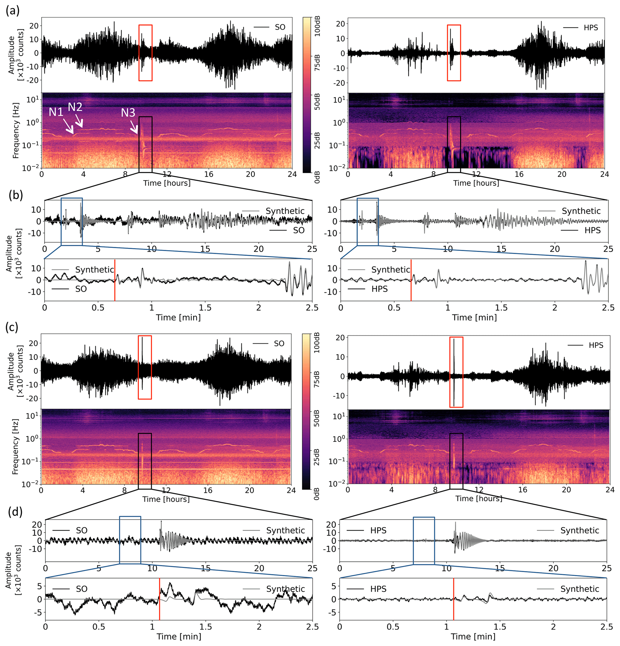
Figure 3Comparison of the synthetic seismograms and spectrograms of the original signal SO and the HPS noise-reduced signal on the R and T components for a synthetic signal with SNR = 1.5 before denoising. Panels (a) and (c) show 1 d seismograms and spectrograms for R and T components, respectively. Squares show the earthquake section. The arrows in (a) show three noise situations (N1–N3). Panels (b) and (d) show seismograms of the earthquake section on SO and HPS signals, with a detailed view of the P arrival (on component R in b) and SH arrival (on component T in d). Red lines show P arrivals in (b) and SH arrival in (d).
Comparing the spectrograms and waveforms of the synthetic example we see a significant improvement of SNR in the HPS processed data set on all components (e.g., Figs. 3 and S3–5 for the real data). The continuous spectral lines of the assumed electronic noise are removed from the data, as are most of the spectral lines related to tremor episodes of head buoy strumming. During the tides, we observe a reduction of the spectral amplitudes for the tilt noise, as well as for the general background noise (Figs. 3 and S3–5) on the horizontal components. The results from the spectrograms are confirmed by the spectra (Fig. 2b), which show the removal of the spectral peaks of the electronic noise (0.05, 0.1, 0.15 Hz) and the tremor episodes (0.5–1 Hz). The amplitude and phase information of the synthetic earthquake is preserved in the HPS signal (see Fig. 3).
To quantify the improvements obtained when using our method, we calculated the cross-correlation of the teleseismic waveform, the SNR of the teleseismic body-wave phases, and the rms of the teleseismic waveform before and after denoising. Because most of the oceanic noise occurs at frequencies below 1 Hz, which is also the most interesting frequency range for the OBS analysis, a 1 Hz low-pass filter is applied to the signals before all result calculations.
We calculated the correlation coefficient for synthetic SO and HPS compared with the synthetic earthquake signal for different SNR and noise realizations and plotted it in Fig. 4a. The high correlation coefficients for HPS and synthetic compared with SO and synthetic in all cases demonstrate a significant noise reduction. Furthermore, they indicate that the HPS denoising preserves the earthquake signal and does not introduce significant waveform distortions since the HPS is more similar to the synthetics compared to SO. In the following we show other measures that confirm the preservation of the earthquake signal.
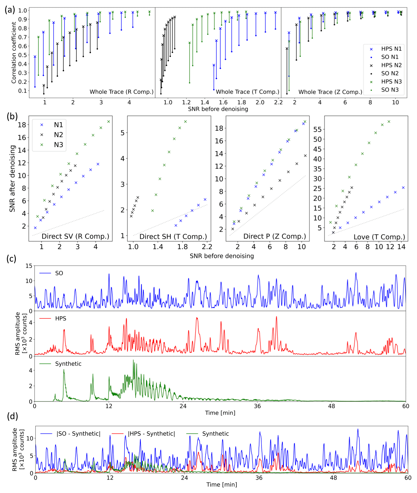
Figure 4Comparison of the synthetic SO and HPS signals (both are low-pass-filtered at 1 Hz). (a) Correlation coefficients (for the whole trace) for different SNRs and three realistic noise realizations for Z, R, and T components (component is abbreviated as Comp.). (b) Improvement of SNR for direct body-wave phases and the Love wave. The gray dotted lines in (b) mark the line with gradient 1 (no improvement of SNR). (c) Comparison of the root mean square (rms) amplitude of one example of the SO, HPS, and synthetic earthquake signals. This signal is the same example shown in Fig. 3 (R component, SNR = 1.5 before denoising). (d) The rms of the original noise (blue trace: | SO – synthetic |) and the remaining noise after denoising (red trace: | HPS – synthetic |) compared to the synthetic earthquake signal.
For the SNR calculation we used a signal window of 30 s starting from the theoretical onset (direct P on Z component, direct S on R and T component, and Love wave on the T component) and a noise window of 60 s starting 70 s before the theoretical onset. For the Love wave, the SV phase (R component), and P phase (Z component) the SNR increased significantly (Fig. 4b). We find that the noise type properties influence the perceived SNR improvement. It appears that there is no SNR improvement on the T component for noise situation N1 (Fig. 4b, the second panel). N1 is taken from the tidal current event's beginning, where there is a significant variation in noise frequencies over time. In this instance, the signal and noise have comparable frequency ranges. Despite the SNR showing no increase, a visual check of the matching trace reveals a definite improvement in the waveform for the SH wave on the T component. The results from the cross-correlation (Fig. 4a) confirm the improvement and preservation of the waveform. The SNR should not be utilized alone to assess the improvement by the HPS noise reduction approach since we are concentrating on the preservation of the waveform and the SNR comparison strongly depends on the noise situation. The improvement of the traces by the HPS noise reduction approach is confirmed by the study of the cross-correlations, rms (which is explained in the following paragraph), and the pure waveforms, even though the SNR does not improve in all instances.
The rms amplitudes of noise-free R-component synthetic, SO, and HPS signals are estimated over 8 s windows with 80 % overlap and plotted in Fig. 4c. Comparing the rms amplitude of the synthetic, SO, and HPS we see that the synthetic and HPS have similar amplitude ranges, while SO has a much higher amplitude. This shows a significant noise reduction in HPS along with preserving the energy of the earthquake and all the phase arrivals. As there is some noise remaining after denoising we see some differences in the overall shapes of the rms amplitude of the synthetic and HPS (especially after minute 24, which is almost at the end of the energy of the synthetic signal). However, HPS shows peaks on the arrival times of seismic phases of the synthetic, which means that the energy of seismic phases is preserved after denoising. The minor changes in seismic phase shapes of the synthetic and HPS are also due to the remaining noise. The seismograms and spectrograms related to this example are presented in Fig. 3. Figure 4d shows a comparison of the rms amplitude of the original noise in SO (blue curve), the remaining noise in HPS after denoising (red curve), and the synthetic earthquake (green curve) signals. Besides a high noise reduction in HPS, the plot shows that the remaining noise is independent of the pattern of the synthetic earthquake, which confirms that the denoising process does not affect the earthquake energy in the HPS signal.
4.2 Applications
By applying our HPS noise reduction algorithm, we aim to improve seismological analyses, especially those involving the analysis of teleseismic body and surface waves. Valuable constraints of the Earth's structure in oceanic regions can be taken from the analysis of the SH wave field like Love waves, which are not influenced by the water column, but often cannot be analyzed due to strong noise on the horizontal components. SV waves are also often masked by noise but are, for instance, important for tomography studies or S and SKS shear wave splitting analysis (e.g., Silver and Chan, 1991). Other techniques using the SV wave field like the Z R ratio of the teleseismic Rayleigh waves (Tanimoto and Rivera, 2008) or receiver functions (RFs) (Langston, 1979) also rely on clear radial component readings. In the following we will show the improvement which was achieved for the SH arrivals and for the group velocity analysis of teleseismic Rayleigh and Love waves, as well as for the receiver function analysis.
4.2.1 SH waves
Since SH waves are weak in energy and displayed on the noise-contaminated transversal horizontal component (T), they are sparsely observable on OBS recordings and are mostly masked by the high noise level. However, on the HPS processed data we see an improvement of the SNR on the T component (see Fig. 4b). In many cases the SH phase is clearly identifiable on the HPS T component (see Fig. 3d for a synthetic data example and Fig. S6 for a real data example).
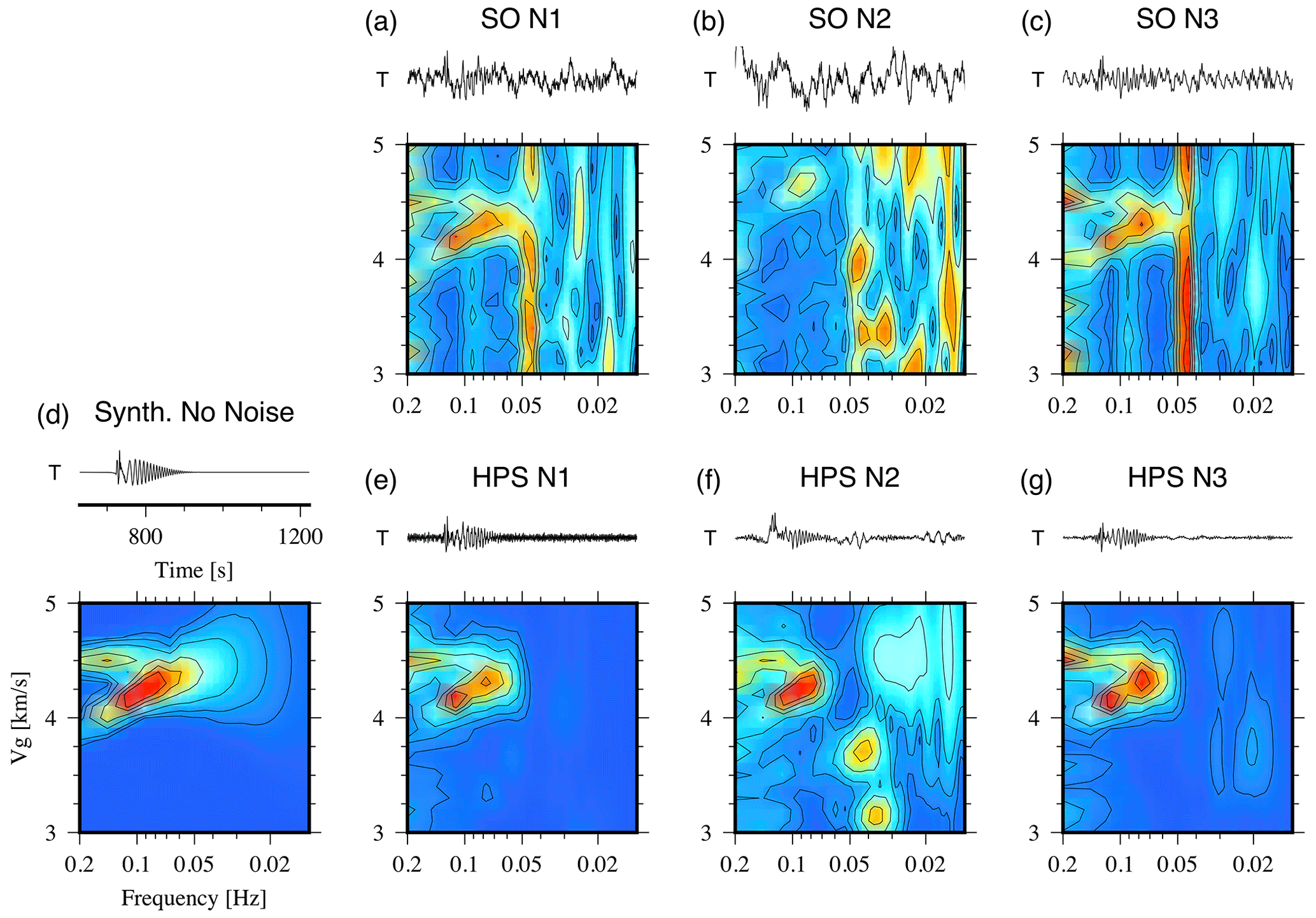
Figure 5Love-wave group velocity analysis for unfiltered and HPS-processed synthetic Love wave trains contaminated by three real-world OBS noise signals (noise situations N1–N3, station D10, DOCTAR experiment, see Sect. 2 for more details). Lower panels in (a)–(c): unfiltered synthetic signal (SO) MFT analysis results. Top panels: seismogram time windows corresponding to the range of group velocities shown on the y axis. (d) Noise-free synthetic case. (e)–(g) HPS-processed input traces for noise situations N1–N3 (lower panel: MFT analysis result, top panel: HPS processed seismogram).
4.2.2 Surface waves
Rayleigh waves in deep oceanic domains are strongly influenced by the water column because most of the wave energy is traveling in the water. This poses a problem if the water depth changes along the travel path. Love waves are not influenced by the water column but are recorded only on horizontal components, and their recordings on OBS systems are therefore more disturbed by strong noise sources like tilt-inducing tidal currents. To test the performance of the HPS noise reduction algorithm in the low-frequency range, we performed a measurement of group velocities of Love and Rayleigh waves with the multiple filter technique (MFT) (Dziewonski et al., 1969). Figure 5 shows group velocity curves for the synthetic Love wave train for the three noise situations N1–N3. For the MFT analysis we used the software mft96 (Herrmann, 2013). The unfiltered seismograms in the top panels (Fig. 5a–c) correspond to the P-wave SNR = 1 scenario. In all three cases the clarity of the dispersion curve is greatly enhanced in the images resulting from the HPS-processed traces (Fig. 5e–g) in comparison to the noise-free image (Fig. 5d). Also, the seismogram traces improved greatly. The dispersion images show how noise energy is successfully removed from the frequency range of 0.05 to 0.2 Hz, which is the event frequency range. The lower-frequency range, which is weakly visible in the noise-free image (Fig. 5d), cannot be recovered. The corresponding results for the Rayleigh wave train on the radial component are shown in Fig. S7. For the N3 case the low-frequency range down to 0.025 Hz can also be successfully denoised.
For an evaluation of the HPS denoising technique on real surface wave data we selected 23 events with magnitudes larger than Mw 6.0 in the distance range between 47.5 and 159.6∘ and added one event with Mw=5.6 at a distance of 37.9∘ (see Fig. S1). Figure S8 shows seismograms and MFT analysis examples for three events with different magnitudes and in different distances. The resulting group velocity dispersion curves for all 24 events for the original and processed data are shown in Fig. S9. For all components we find that the improved signal-to-noise ratio of the processed data allows the analysis of more events and of a broader frequency range than in the original data.
4.2.3 Receiver functions
Receiver functions have been proven to be a valuable tool to observe the Earth's structure using teleseismic events (e.g., Langston, 1979; Ammon et al., 1995; Kind et al., 1995; Rondenay, 2009). Separating the source site from the receiver site by deconvolution allows estimating the Earth's structure beneath the station. Here, we compare the receiver functions calculated from the synthetic examples and from real data before and after denoising (Fig. 6). The synthetics used for the receiver function calculation are pure synthetic signals contaminated by real noise (N1, N2, N3). On the synthetics, the SNR for P ranges between 1 and 10 (for a detailed description of the synthetic creation, see Sect.4.1, Figs. 3 and S2). Receiver function analysis and the observation of the Earth's structure beneath the DOCTAR array were already conducted by Hannemann et al. (2017). Here, we do not aim to estimate the crustal and mantle structures; instead, we aim to compare the P-receiver functions of the radial component calculated from the original synthetic and real data (SO R-RF) with receiver functions of the radial component from the HPS processed synthetic and real data (HPS R-RF). To calculate the receiver functions, we applied the iterative deconvolution in the time domain (Ligorría and Ammon, 1999). We corrected the data for the Ps phase, quality-controlled (e.g., P onset at 0 s on Z of HPS R-RF), stacked, and low-pass-filtered the synthetic data at 2 Hz, and bandpass-filtered the traces between 0.05 and 0.5 Hz for the real data with a zero-phase Butterworth filter. For both the synthetic and real receiver function, the noise level strongly decreased, and we observe a significant decrease in variance on the HPS traces compared to the SO traces (Fig. 6).
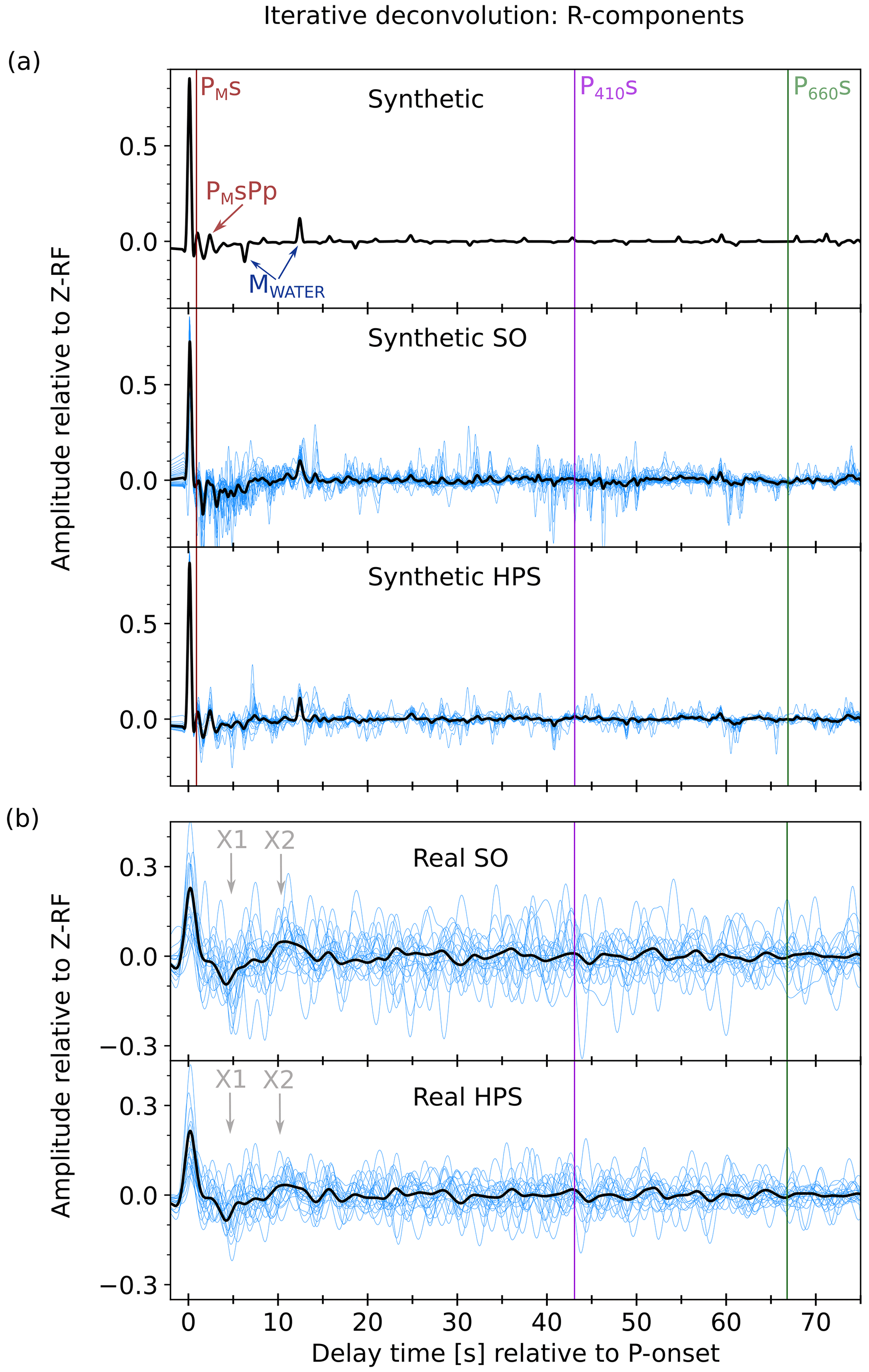
Figure 6R-receiver function comparison of synthetic and real data examples. (a) Comparison of the synthetic data examples, low-pass-filtered at 2 Hz. The pure synthetic R-RF is shown in the uppermost panel, followed by the synthetic SO and the synthetic HPS R-RFs. The black lines show the summed individual R-RFs (blue waveforms). The theoretical onset times for this specific model are marked. Red line: Ps arrival of the Moho (PMs) and its multiple (PMsPp), violet line: Ps arrival of the 410 (P410s), green line: Ps arrival of the 660 (P660s), dark blue arrows: multiples in the water column of 4.9 km (MWATER), repetitive every 6.5 s. (b) Comparison of the real data, bandpass-filtered at 0.05–0.5 Hz. The upper panel shows the R-RFs of the real SO traces and the lowermost panel the R-RFS of the real HPS traces. The individual traces (blue) are shown as a stack (black line), and the theoretical onset times based on the average ak135 velocity model are shown as a violet line (P410s) and green line (P660s). The origin of the phases X1 and X2 (gray) remains unclarified, since their interpretation is beyond the scope of this study.
Our result shows that determination of the crustal and mantle phases is more reliable on the HPS R-RF stack than on the SO R-RF stack for both synthetic and real data (Fig. 6). We observe more distinct Ps-phase arrivals on the HPS R-RF than on the SO R-RF stack. The Ps phases are caused by the P-to-S conversion at the Mohorovičić, 410, and 660 km discontinuity (hereafter referred to as Moho, 410, and 660, respectively; e.g., Deuss, 2009). For the synthetic example, we expect the P-to-S conversion at the Moho at depths of 11.5 km to arrive at 0.8 s, which is better resolved in the synthetic HPS R-RF than in the synthetic SO R-RF; the same is true for its multiple (PMsPp) and the water multiples every 6.5 s (MWATER, Fig. 6a).
Assuming ak135 velocities we would expect the P410s phase (Ps conversion at the 410) to arrive at around 43 s and the P660s phase (Ps conversion at the 660) at around 66.8 s delayed compared to the direct P arrival (see Fig. 6a and b).
Instead of a rather weak peak on the SO R-RF real data stack we observe a strong peak at around 43 s, with a good SNR on the HPS R-RF stack, indicating the sharp velocity contrast at the 410 (Fig. 6b). Comparing SO RF and HPS RF real data stacks, the amplitudes of the P660s phase on the HPS decreased and became a broader peak. This aligns with our expectations from a conversion at a gradual velocity contrast as at the 660. These results are in line with the analysis of the crustal and mantle structure beneath the DOCTAR array presented by Hannemann et al. (2017). The negative phase (X1 in Fig. 6b) arriving at around 5 s is stronger on the HPS R-RF real data stack than on the SO R-RF real data stack and might indicate either the PpSs multiple of the Ps phase at the Moho or the direct P-to-S lithosphere–asthenosphere boundary (LAB). On the HPS R-RF real data stack we observe a strong positive phase (X2) arriving at 12 s (Fig. 6b). This phase was not identified by Hannemann et al. (2017), and a detailed analysis of its origin is beyond the scope of this study, but it might be related to the water multiples.
In this work we have developed a method to separate the signals of teleseismic earthquakes from other signals in OBS recordings, resulting in noise reduction of OBS data. Our method is a combination of two HPS algorithms from the field of music information retrieval (MIR) to separate harmonic and percussive components of OBS data. Earthquake signals as percussive components are separated from noise signals as harmonic components. The noise signal is reconstructed using the phase information of the original signal. Subtracting the noise signal from the original signal derives the noise-reduced signal. Our two-step HPS approach results in a cleaner, noise-reduced signal wherein the teleseismic broadband earthquake waveforms are preserved with their whole frequency content. Our synthetic tests show that the SNR of HPS noise-reduced signal significantly increases in most cases; however, the apparent SNR improvement depends on the noise type characteristics. The types of noise signals, which are eligible for our noise reduction algorithm, contain most of the OBS noise energy.
The extracted noise signal contains some different signals; each can be derived by applying a bandpass filter to the extracted noise signal in a proper frequency band. The derived signal may be used in research related to that signal. For example, the microseism signal can be extracted and used for investigation of the source generation area of microseisms.
From our analysis of the broadband seismograms, we find that the improvement is significant and allows a broader and more reliable analysis of teleseismic earthquake data. Applications like the receiver function technique as well as SH-wave and Love-wave analysis are considerably improved after applying the HPS noise reduction algorithm.
Group velocity analysis of teleseismic surface wave trains showed that application of the HPS noise reduction technique allows analyzing more events and analyzing them in a broader frequency range. More and wider Love-wave dispersion curves could be recovered. The noise reduction algorithm improves the horizontal components significantly, which allows the OBS community to apply a broader range of seismological methodologies, including the horizontal components, to the OBS data.
A Python package named NoiseCut (https://doi.org/10.5281/zenodo.7339552, Zali, 2022) and the code related to the proposed method along with an example of real data are freely available from https://github.com/ZahraZali/NoiseCut (last access: November 2022). The average computation time for this example (1 d OBS signal with a sampling frequency of 100 Hz) is about 7 min on a PC with an Intel core i7 (six-core) processor of 2.2 GHz and 16 GB of RAM. A Jupyter notebook with all the Python codes and parameters related to the proposed method is available as an electronic Supplement. The seafloor seismological data were archived by the Alfred Wegener Institute (AWI), Helmholtz Centre for Polar Research, Bremerhaven, Germany, and are available upon request. The Supplement related to this article contains a list of all earthquakes used in this study and a map showing their location. The illustrations of the semi-synthetic data generation are presented in the Supplement as well. Examples of a three-component seismogram and spectrogram before and after applying the HPS noise reduction algorithm to real data, Rayleigh-wave group velocity analysis for a synthetic example, MFT analysis for three real events, and group velocity curves for some real events are also presented in figures in the Supplement. For building our method, we used Librosa, a Python package for audio and music signal processing (https://doi.org/10.5281/zenodo.7657336, McFee et al., 2023). The data processing was done using obspy (Beyreuther et al., 2010) and pyrocko (Heimann et al., 2017); the receiver functions were calculated using the rf package (Eulenfeld, 2020).
The supplement related to this article is available online at: https://doi.org/10.5194/se-14-181-2023-supplement.
ZZ developed the algorithm and designed the study. TR created the synthetic data, conducted the synthetic tests, and measured the receiver functions. FK conducted the group velocity analysis. ZZ, TR, and FK evaluated the results. ZZ and TR wrote the initial draft. All authors wrote the final paper and discussed the results.
The contact author has declared that none of the authors has any competing interests.
Publisher's note: Copernicus Publications remains neutral with regard to jurisdictional claims in published maps and institutional affiliations.
The seafloor seismological data were archived by the Alfred Wegener Institute (AWI), Helmholtz Centre for Polar Research, Bremerhaven, Germany, and are available upon request. We acknowledge the DEutscher Geräte-Pool für Amphibische Seismologie (DEPAS) (Schmidt-Aursch and Haberland, 2017) that is currently the largest European OBS pool. We acknowledge Sebastian Heimann for helping package the code related to the method. The authors would like to thank the editor Simone Pilia and two anonymous reviewers for their insightful comments.
This research has been supported by the Deutscher Akademischer Austauschdienst (grant no. 91721165) and the Deutsche Forschungsgemeinschaft (grant nos. DFG MU 2686/13-1, SCHE 280/20-1).
This paper was edited by Simone Pilia and reviewed by two anonymous referees.
Ammon, C. J., Randall, G. E., and Zandt, G.: On the nonuniqueness of receiver function inversions, J. Geophys. Res.-Sol. Ea., 95, 15303–15318, https://doi.org/10.1029/JB095iB10p15303, 1990.
An, C., Cai, C., Zhou, L., and Yang, T.: Characteristics of Low-Frequency Horizontal Noise of Ocean-Bottom Seismic Data, Seismol. Res. Lett., 93, 257–267. https://doi.org/10.1785/0220200349, 2021.
Bell, S. W., Forsyth, D. W., and Ruan, Y.: Removing noise from the vertical component records of ocean-bottom seismometers: Results from year one of the Cascadia Initiative, B. Seismol. Soc. Am., 105, 300–313, https://doi.org/10.1785/0120140054, 2015.
Beyreuther, M., Barsch, R., Krischer, L., Megies, T., Behr, Y., and Wassermann, J.: ObsPy: A Python Toolbox for Seismology. Seismol. Res. Lett., 81, 530–533, 2010.
Brink, K. H.: Tidal and lower frequency currents above Fieberling Guyot, J. Geophys. Res.-Oceans, 100, 10817–10832, https://doi.org/10.1029/95JC00998, 1995.
Corela, C.: Ocean bottom seismic noise: applications for the crust knowledge, interaction ocean-atmosphere and instrumental behaviour, PhD thesis, University of Lisbon, 339 pp., http://hdl.handle.net/10451/15805, 2014.
Crawford, W. C.: Determination of oceanic crustal shear velocity structure from seafloor compliance measurements, Doctoral dissertation, University of California, San Diego, https://www.ipgp.fr/~crawford/Homepage/Publis/Crawford1994_Thesis.pdf (last access: July 2002), 1994.
Crawford, W. C. and Webb, S. C.: Identifying and removing tilt noise from low-frequency (< 0.1 Hz) seafloor vertical seismic data, B. Seismol. Soc. Am., 90, 952–963, https://doi.org/10.1785/0119990121, 2000.
Crawford, W. C., Webb, S. C., and Hildebrand, J. A.: Estimating shear velocities in the oceanic crust from compliance measurements by two-dimensional finite difference modeling, J. Geophys. Res.-Sol. Ea., 103, 9895–9916, https://doi.org/10.1029/97JB03532, 1998.
Deuss, A.: Global observations of mantle discontinuities using SS and PP precursors, Surv. Geophys., 30, 301–326, https://doi.org/10.1007/s10712-009-9078-y, 2009.
Driedger, J., Müller, M., and Disch, S.: Extending Harmonic-Percussive Separation of Audio Signals, in: ISMIR, 611–616, https://doi.org/10.5281/zenodo.1415226, 2014.
Duennebier, F. K. and Sutton, G. H.: Fidelity of ocean bottom seismic observations, Oceanographic Literature Review, 10, 996, https://doi.org/10.1007/BF01204343, 1995.
Dziewonski, A., Bloch, S., and Landisman, M.: A technique for the analysis of transient seismic signals, B. Seismol. Soc. Am., 59, 427–444, https://doi.org/10.1785/BSSA0590010427, 1969.
Essing, D., Schlindwein, V., Schmidt-Aursch, M. C., Hadziioannou, C., and Stähler, S. C.: Characteristics of Current-Induced Harmonic Tremor Signals in Ocean-Bottom Seismometer Records, Seismol. Res. Lett., 92, 3100–3112, https://doi.org/10.1785/0220200397, 2021.
Eulenfeld, T.: rf: Receiver function calculation in seismology, J. Open Source Softw., 5, 1808, https://doi.org/10.21105/joss.01808, 2020.
Fitzgerald, D.: Harmonic/percussive separation using median filtering, in: Proceedings of the International Conference on Digital Audio Effects (DAFx), Vol. 13, https://doi.org/10.1049/ic.2012.0225, 2010.
FitzGerald, D.: Vocal separation using nearest neighbours and median filtering, 23rd IET Irish Signals and Systems Conference, Maynooth, 28–29 June 2012, https://doi.org/10.1049/ic.2012.0225, 2012.
Friedrich, A., Krüger, F., and Klinge, K.: Ocean-generated microseismic noise located with the Gräfenberg array, J. Seismol., 2, 47–64, https://doi.org/10.1023/A:1009788904007, 1998.
Hannemann, K., Krüger, F., Dahm, T., and Lange, D.: Oceanic lithospheric S wave velocities from the analysis of P wave polarization at the ocean floor, Geophys. J. Int., 207, 1796–1817, https://doi.org/10.1093/gji/ggw342, 2016.
Hannemann, K., Krüger, F., Dahm, T., and Lange, D.: Structure of the oceanic lithosphere and upper mantle north of the Gloria fault in the eastern mid-Atlantic by receiver function analysis, J. Geophys. Res.-Sol. Ea., 122, 7927–7950, https://doi.org/10.1002/2016JB013582, 2017.
Hasselmann, K.: A statistical analysis of the generation of microseisms, Rev. Geophys., 1, 177–210, https://doi.org/10.1029/RG001i002p00177, 1963.
Heimann, S., Kriegerowski, M., Isken, M., Cesca, S., Daout, S., Grigoli, F., Juretzek, C., Megies, T., Nooshiri, N., Steinberg, A., Sudhaus, H., Vasyura-Bathke, H., Willey, T., and Dahm, T.: Pyrocko – An open-source seismology toolbox and library, V. 0.3, GFZ Data Services [data set], https://doi.org/10.5880/GFZ.2.1.2017.001, 2017.
Herrmann, R. B.: Computer programs in seismology: An evolving tool for instruction and research, Seismol. Res. Lett., 84, 1081–1088, https://doi.org/10.1785/0220110096, 2013.
Janiszewski, H. A., Gaherty, J. B., Abers, G. A., Gao, H., and Eilon, Z. C.: Amphibious surface-wave phase-velocity measurements of the Cascadia subduction zone, Geophys. J. Int., 217, 1929–1948, https://doi.org/10.1093/gji/ggz051, 2019.
Johnson, J. B., and Watson, L. M.: Monitoring volcanic craters with infrasound “music”, Eos, 100, https://doi.org/10.1029/2019EO123979, 2019.
Kennett, B. L., Engdahl, E. R., and Buland, R.: Constraints on seismic velocities in the Earth from traveltimes, Geophys. J. Int., 122, 108–124, https://doi.org/10.1111/j.1365-246X.1995.tb03540.x, 1995.
Kind, R., Kosarev, G. L., and Petersen, N. V.: Receiver functions at the stations of the German Regional Seismic Network (GRSN), Geophys. J. Int., 121, 191–202, https://doi.org/10.1111/j.1365-246X.1995.tb03520.x, 1995.
Langston, C. A.: Structure under Mount Rainier, Washington, inferred from teleseismic body waves, J. Geophys. Res., 84, 4749–4762, https://doi.org/10.1029/JB084iB09p04749, 1979.
Ligorría, J. P. and Ammon, C. J.: Iterative deconvolution and receiver-function estimation, B. Seismol. Soc. Am., 89, 1395–1400, https://doi.org/10.1785/BSSA0890051395, 1999.
McFee, B., McVicar, M., Faronbi, D., et al.: librosa/librosa: 0.10.0 (0.10.0), Zenodo [code], https://doi.org/10.5281/zenodo.7657336, 2023.
Mousavi, S. M. and Langston, C.A.: Automatic noise-removal/signal-removal based on general cross-validation thresholding in synchrosqueezed domain and its application on earthquake data, Geophysics, 82.4, V211–V227, https://doi.org/10.1190/geo2016-0433.1, 2017.
Müller, M.: Fundamentals of music processing: Audio, analysis, algorithms, applications, Cham, Switzerland: Springer International Publishing, https://doi.org/10.1007/978-3-319-21945-5, 2015.
Negi, S. S., Kumar, A., Ningthoujam, L. S., and Pandey, D. K.: An Efficient Approach of Data Adaptive Polarization Filter to Extract Teleseismic Phases from the Ocean-Bottom Seismograms, Seismol. Soc. Am., 92, 528–542, https://doi.org/10.1785/0220200034, 2021.
Rafii, Z. and Pardo, B.: Music/Voice Separation Using the Similarity Matrix, Proc. ISMIR, 583–588, 2012.
Rafii, Z., Liutkus, A., and Pardo, B.: REPET for background/foreground separation in audio, in: Blind Source Separation, Springer, Berlin, Heidelberg, 395-411, https://doi.org/10.1007/978-3-642-55016-4_14, 2014.
Rafii, Z., Liutkus, A., Stöter, F. R., Mimilakis, S. I., FitzGerald, D., and Pardo, B.: An overview of lead and accompaniment separation in music, IEEE T. Audio Speech, 26, 1307–1335, https://doi.org/10.1109/TASLP.2018.2825440, 2018.
Ramakrushana Reddy, T., Dewangan, P., Arya, L., Singha, P., and Kamesh Raju, K. A.: Tidal triggering of the harmonic noise in ocean-bottom seismometers, Seismol. Res. Lett., 91, 803–813, https://doi.org/10.1785/0220190080, 2020.
Rondenay, S.: Upper mantle imaging with array recordings of converted and scattered teleseismic waves, Surv. Geophys., 30, 377–405, https://doi.org/10.1007/s10712-009-9071-5, 2009.
Romanowicz, B., Stakes, D., Montagner, J. P., Tarits, P., Uhrhammer, R., Begnaud, M., Stutzmann, E., Pasyanos, M., Karczewski, J. F., Etchemendy, S., and Neuhauser, D.: MOISE: A pilot experiment towards long term sea-floor geophysical observatories, Earth Planets Space, 50, 927–937, https://doi.org/10.1186/BF03352188, 1998.
Schlindwein, V., Wassermann, J., and Scherbaum, F.: Spectral analysis of harmonic tremor signals at Mt. Semeru volcano, Indonesia, Geophys. Res. Lett., 22, 1685–1688, https://doi.org/10.1029/95GL01433, 1995.
Schlindwein, V., Krüger, F., and Schmidt-Aursch, M.: Project KNIPAS: DEPAS ocean-bottom seismometer operations in the Greenland Sea in 2016-2017, Alfred Wegener Institute, Helmholtz Centre for Polar and Marine Research, Bremerhaven, PANGAEA [data set], https://doi.org/10.1594/PANGAEA.896635, 2018.
Schmidt-Aursch, M. and Haberland, C.: DEPAS (Deutscher Geräte-Pool für amphibische Seismologie): German instrument pool for amphibian seismology, J. Largescale Res. Facil., 3, A122, https://doi.org/10.17815/jlsrf-3-165, 2017.
Silver, P. G. and Chan, W. W.: Shear wave splitting and subcontinental mantle deformation, J. Geophys. Res., 96, 16429–16454, https://doi.org/10.1029/91JB00899, 1991.
Stähler, S. C., Schmidt-Aursch, M. C., Hein, G., and Mars, R.: A self-noise model for the German DEPAS OBS pool, Seismol. Res. Lett., 89, 1838–1845, https://doi.org/10.1785/0220180056, 2018.
Tanimoto, T. and Rivera, L.: The ZH ratio method for long-period seismic data: sensitivity kernels and observational techniques, Geophys. J. Int., 172, 187–198, https://doi.org/10.1111/j.1365-246X.2007.03609.x, 2008.
Vaseghi, S. V.: Advanced signal processing and digital noise reduction, Vieweg + Teubner Verlag, https://doi.org/10.1002/9780470740156, 1996.
Wang, R.: A simple orthonormalization method for stable and efficient computation of Green's functions, B. Seismol. Soc. Am., 89, 733–741, https://doi.org/10.1785/BSSA0890030733, 1999.
Webb, S. C.: Broadband seismology and noise under the ocean, Rev. Geophys., 36, 105–142, https://doi.org/10.1029/97RG02287, 1998.
Webb, S. C., Zhang, X., and Crawford, W.: Infragravity waves in the deep ocean, J. Geophys. Res.-Oceans, 96, 2723–2736, https://doi.org/10.1029/90JC02212, 1991.
Zali, Z.: ZahraZali/NoiseCut: NoiseCut (v1.0.0), Zenodo [code], https://doi.org/10.5281/zenodo.7339552, 2022.
Zali, Z., Ohrnberger, M., Scherbaum, F., Cotton, F., and Eibl, E. P.: Volcanic Tremor Extraction and Earthquake Detection Using Music Information Retrieval Algorithms, Seismol. Res. Lett., 92, 3668–3681, https://doi.org/10.1785/0220210016, 2021.
Zhu, W., Mousavi, S. M., and Beroza, G. C.: Seismic signal denoising and decomposition using deep neural networks, IEEE T. Geosci. Remote., 57, 9476–9488, https://doi.org/10.1109/TGRS.2019.2926772, 2019.