ECOMAN: an open-source package for geodynamic and seismological modelling of mechanical anisotropy

Mechanical anisotropy related to rock fabrics is a proxy for constraining the Earth's deformation patterns. However, the forward and inverse modelling of mechanical anisotropy in 3D large-scale domains has been traditionally hampered by the intensive computational cost and the lack of a dedicated, open-source computational framework. Here we introduce ECOMAN (Exploring the COnsequences of Mechanical ANisotropy), a software package for modelling strain- and stress-induced rock fabrics and testing the effects of the resulting elastic and viscous anisotropy on seismic imaging and mantle convection patterns.

Differently from existing analogous software, ECOMAN can model strain-induced fabrics across all mantle levels and is optimised to run efficiently on multiple CPUs. It also enables modelling of shape preferred orientation (SPO)-related structures that can be superimposed over lattice/crystallographic preferred orientation (LPO/CPO) fabrics, which allows the consideration of the mechanical effects of fluid-filled cracks, foliated and lineated grain-scale fabrics, and rock-scale layering.

One of the most important innovations is the Platform for Seismic Imaging (PSI), a set of programs for performing forward and inverse seismic modelling in isotropic–anisotropic media using real or synthetic seismic datasets. The anisotropic inversion strategy is capable of recovering parameters describing a tilted transversely isotropic (TTI) medium, which is required to reconstruct 3D structures and mantle strain patterns and to validate geodynamic models.

1 Introduction

The study of the Earth's interior has been traditionally based on seismological and geodynamic modelling, the former providing important information about its present-day structure, composition, and state (Chang et al., 2015; French and Romanowicz, 2015; Schaeffer et al., 2016; Debayle et al., 2020) and the latter about its dynamics and compositional evolution (Davies et al., 2012; Crameri and Tackley, 2014; Müller et al., 2022). Seismological modelling and geodynamical modelling are very often conducted independently, which creates mechanical and geometrical inconsistencies across the models, hampers the interpretation of seismic observations in terms of geodynamic processes, and exacerbates the non-uniqueness of geodynamic model predictions. An alternative approach is combining computational seismology and geodynamics with mineral physics, which provides a comprehensive understanding of the Earth's interior processes, seismic behaviour, and material properties. This multidisciplinary methodology has been used in previous studies to post-process geodynamic flow calculations with thermodynamically self-consistent models of mantle mineralogy and convert thermal structure into isotropic elastic parameters. The obtained seismic mantle structure can then be used in simulations of global wave propagation such that specific hypotheses on mantle dynamics can be tested directly against seismic data (Styles et al., 2011; Schuberth et al., 2012; Maguire et al., 2018). The inverse procedure consists of converting seismic anomalies into density anomalies driving mantle flow models and is typically employed to quantify dynamic topography and mantle viscosity structure, as well as to reproduce large-scale mantle flow patterns (e.g. Bunge et al., 2003; Steinberger and Calderwood, 2006; Rudolph et al., 2015). However, isotropic seismic imaging provides limited information regarding local- and regional-scale dynamical processes (Fraters and Billen, 2021), and a better way to couple the geodynamic evolution and seismological structure of the Earth's interior is by accounting for the strain- and stress-induced mechanical anisotropy of crustal and mantle rocks.

Mechanical anisotropy refers to the directional dependence of mechanical properties in a material and is well known to affect both elastic and viscous deformational behaviour. Mechanical anisotropy depends on several factors, including the lattice or crystal preferred orientation (LPO, CPO) of intrinsically anisotropic minerals and extrinsic mechanisms related to the shape preferential orientation (SPO) of melt, fluid, or air-filled fractures and non-spherical pores, as well as grain- or rock-scale compositional layering. Most micro- and macro-scale fabrics are acquired as a function of the cumulative deformation and material mechanical properties, and as such they constitute an important source of information about the Earth's dynamical behaviour.

Elastic anisotropy is directly connected to seismic anisotropy, which is a phenomenon in which the seismic wave speed varies as a function of the propagation direction. It is mainly observed in the crust, mantle boundary layers, and inner core (Almqvist and Mainprice, 2017; Karato, 1998; Kendall, 2000; Long and Becker, 2010; Deuss, 2014). Understanding and modelling seismic anisotropy are crucial for determining long-term deformational patterns and the present-day stress field in the crust, as well as constraining geodynamic modelling predictions (Jadamec and Billen, 2010; Hu et al., 2017; Zhou et al., 2018; Lo Bue et al., 2022). In addition, the ability to account for anisotropic effects can improve the quality of subsurface imaging. Indeed, it has been demonstrated that, because of uneven seismic ray coverage, failing to account for seismic anisotropy may generate strong artefacts that substantially bias our understanding of mantle structures and dynamics in different tectonic settings (Bezada et al., 2016; VanderBeek and Faccenda, 2021; VanderBeek et al., 2023; Faccenda and VanderBeek, 2023). Considering the widespread presence of seismic anisotropy, anisotropic seismic models provide a more realistic representation of the Earth's subsurface compared to isotropic models.

Viscous anisotropy modelling refers to the study and simulation of materials that exhibit varying degrees of viscosity (resistance to viscous deformation) in different directions. Although viscous anisotropy has been traditionally associated with the mechanical behaviour of multi-layered media (Mühlhaus et al., 2002; Kocher et al., 2006), it has been also observed in experimentally deformed mica-rich and olivine crystal aggregates (Shea and Kronenberg, 1993; Hansen et al., 2014). Previous numerical studies demonstrated that viscous anisotropy can potentially stabilise long-wavelength convective patterns (Christensen, 1987; Mühlhaus et al., 2004) and more generally affect processes such as plate motion (Király et al., 2020), post-glacial rebound (Han and Wahr, 1997), lithospheric shear zone reactivation (Tommasi et al., 2009), and dripping (Lev and Hager, 2008a).

Over the last few years a few attempts have been made to integrate micro-mechanical modelling of fabric evolution with large-scale geodynamic models using either directors (Lev and Hager, 2008b; Halter et al., 2022), the CPO model D-REX (Kaminski et al., 2004; Becker et al., 2006; Jadamec and Billen, 2010; Faccenda and Capitanio, 2013; Faccenda, 2014; Ito et al., 2014; Hu et al., 2017; Zhou et al., 2018; Fraters and Billen, 2021), or the CPO model viscoplastic self-consistent (VPSC; Tommasi et al., 2009; Li et al., 2014). However, each of these methodologies has its own limitations mainly associated with the accuracy of the estimates, the large computational burden, or software accessibility, which have impeded a more widespread diffusion in the geodynamic community. At the same time, the recovery of 3D seismic anisotropy patterns has been traditionally considered intractable due to the highly underdetermined nature of the inverse problem, and, although it has been addressed by several previous studies (e.g. Debayle et al., 2005; Panning and Romanowicz, 2006; Abt and Fischer, 2008; Long et al., 2008; Wookey, 2012; Mondal and Long, 2019), only recently have a theoretical background and computational algorithms been developed to simultaneously invert for P- and/or S-wave isotropic velocity anomalies and anisotropy resulting from arbitrarily oriented structures (Munzarova et al., 2018; VanderBeek and Faccenda, 2021; Rappisi et al., 2022; Wang and Zhao, 2021; VanderBeek et al., 2023; Del Piccolo et al., 2024). Yet, to date there is no freely available software capable of modelling seismic anisotropy related to arbitrarily oriented structures.

In this contribution we present the new and open-source software package ECOMAN (Exploring the COnsequences of Mechanical ANisotropy) that enables linking seismology and geodynamics by providing a set of computationally optimised programs for (i) estimating rock mechanical anisotropy as a function of the geodynamic model deformation history and compositional, rheological, stress, pressure, and temperature fields and (ii) solving forward and inverse seismological problems accounting for seismic anisotropy. In the next sections, we first describe the different ECOMAN modules, after which we discuss the advantages and limitations of the software package and the roadmap for future developments.

Table 1 Abbreviations and their description. Units are indicated for dimensional physical properties.

2 Software package structure

ECOMAN includes several programs that are complementary and can be grouped into three main categories (Fig. 1):

1. programs that estimate strain- and stress-induced rock fabrics (LPO and SPO) and their elastic and viscous anisotropic mechanical properties (D-REX_S, D-REX_M, EXEV);

2. programs that post-process the simulated rock fabrics for visualisation of their isotropic–anisotropic mechanical properties and deformational history (VIZTOMO, VIZVISC) and format the elastic tensors generating input files for seismological synthetics (VIZTOMO); and

3. programs that test the elastic response of anisotropic media by performing seismological forward and inverse modelling and, in particular, isotropic and anisotropic seismic tomographies on synthetic and real seismic datasets (SKS-SPLIT, PSI).

Most of the code modules are written in the Fortran programming language, except for the PSI program that is written in Julia. Visualisation of the output is done through the MATLAB MTEX toolbox (Mainprice et al., 2011) for single-aggregate fabrics and ParaView (Ahrens et al., 2005) for 2D and 3D simulations.

Figure 1 ECOMAN structure and flowchart. Coloured boxes denote programs that compute rock fabrics (green); post-process the elastic (C), viscous (η), and deformation gradient (F) tensors for visualisation and/or data formatting for seismological synthetics (orange); and perform seismological forward and inverse modelling on synthetic or real datasets (yellow). Input data are from geodynamic modelling or real seismic datasets (blue). Visualisation of the mechanical properties and LPO can be done with the MTEX MATLAB toolbox for single-crystal aggregates or the software ParaView for large-scale simulations.

2.1 Rock fabric and mechanical property simulations

The evolution of the strain-induced LPO can be simulated with the D-REX model (Kaminski et al., 2004), which has been adapted to reproduce the fabric evolution of single (D-REX_S) or multiple (D-REX_M) two-mineral-phase aggregates representative of the entire Earth's mantle. The accuracy of the D-REX model has been tested against analytical solutions derived by Fraters and Billen (2021) (Appendix A). Five sets of two-mineral-phase mantle aggregates can be defined as a function of depth or density ρ (Fig. 2; see Table 1 for a list of abbreviations and physical properties):

1. olivine + enstatite for the upper mantle (UM: 0–410 km or $\mathrm{3000}<\mathit{\rho }\le \mathrm{3650}$ kg m⁻³);

2. wadsleyite + majoritic garnet for the upper mantle transition zone (UTZ: 410–520 km or $\mathrm{3650}<\mathit{\rho }\le \mathrm{3870}$ kg m⁻³);

3. ringwoodite + majoritic garnet for the lower mantle transition zone (LTZ: 520–660 km or $\mathrm{3870}<\mathit{\rho }\le \mathrm{4150}$ kg m⁻³);

4. bridgmanite + ferropericlase for the lower mantle (LM: 660–2900 km or ρ>4150 kg m⁻³);

5. post-perovskite + ferropericlase for the bottom of the lower mantle according to the parameterised phase boundary $P\left(\mathrm{GPa}\right)=\mathrm{98.7}+T\left(\mathrm{K}\right)\cdot \mathrm{0.00956}$ (Oganov and Ono, 2004).

The strain-induced LPO is computed for the phases in bold, while other major phases such as garnet, ringwoodite, and ferropericlase are considered to be isotropic and their distribution is set to be random. Thus, no LPO is calculated for the LTZ such that (minor) anisotropy arises only when SPO modelling due to compositional layering is active (Sect. 2.1.3; Faccenda et al., 2019). The LPOs of wadsleyite, bridgmanite, and post-perovskite are computed according to the same D-REX methodology originally applied to upper-mantle phases and described in detail in Kaminski and Ribe (2001) and Kaminski et al. (2004) but including additional slip systems as indicated in Table A1. For each of these new phases it is possible to define in the D-REX_S and D-REX_M input files the same free parameters of the D-REX model (the dimensionless grain boundary mobility M^*, nucleation parameter λ^*, threshold volume fraction χ, and in addition the power-law exponent for dislocation creep deformation within the grains) as for upper-mantle aggregates. The full elastic tensor is then calculated according to the crystal orientation, volume fraction, phase abundance, P–T conditions, and bulk rock composition, as well as using Voigt–Reuss–Hill averaging schemes (see Sect. 2.1.2 and Appendix B for more details).

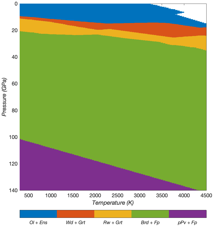
Figure 2 Two-phase aggregates defined by the density crossovers and Brd–pPv phase transition for a pyrolytic mantle composition.

The elastic properties related to strain- and stress-induced SPO fabrics can instead be calculated at the grain or rock scale and for layered or two-phase (matrix-ellipsoidal inclusions) systems using the isotropic elastic moduli of the different (fluid, mineral, rock) components (EXEV).

The elastic properties and density of the aggregates characterised by LPO and/or SPO fabrics are estimated at relevant mantle P–T conditions using the single-crystal elastic moduli and their P–T derivatives for the main mineral phases and compiled from different mineral physics studies, together with lookup tables of the isotropic elastic moduli, density, and mineral-phase volume fraction generated with MMA_EoS (Chust et al., 2017) for five bulk rock compositions (dunite, harzburgite, pyrolite, MORB, pyroxenite) at temperature and pressure ranges of $T=\mathrm{300}:\mathrm{50}:\mathrm{4500}$ K and $P=\mathrm{0}:\mathrm{0.1}:\mathrm{140}$ GPa, respectively (see Appendix B and Tables B1 and B2).

2.1.1 D-REX_S

D-REX_S is a program designed for modelling the evolution of strain-induced LPO fabrics and related elastic properties of a single, two-mineral-phase mantle aggregate as a function of the imposed flow field, amount of strain, crystal plasticity, P–T conditions, and additional effects related to SPO fabrics. It builds on the original D-REX software (Kaminski et al., 2004) for modelling the strain-induced LPO, and it includes MATLAB scripts to generate pole figures of the LPO and isotropic–anisotropic seismic properties with the MTEX software (Mainprice et al., 2011) (Fig. 3a–d), together with the possibility to display the evolving fabric strength (M index, J index) and the fraction of different anisotropy components (obtained via tensor decomposition; Browaeys and Chevrot, 2004; Fig. 3e–h).

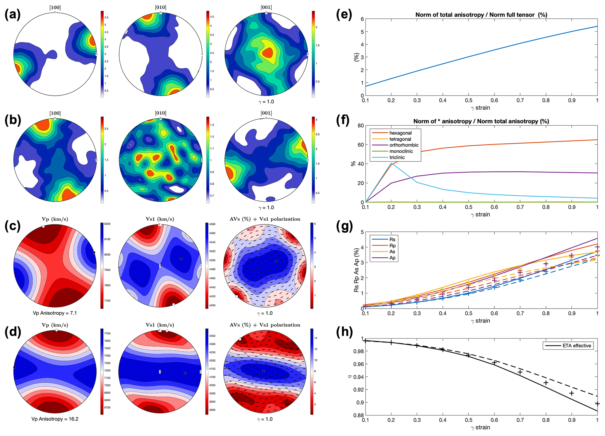
Figure 3 D-REX_S output for an upper-mantle aggregate ($\mathrm{Ol}:\mathrm{Opx}=\mathrm{70}:\mathrm{30}$) subjected to a simple shear deformation of (1) pole figures of the olivine (a) and orthopyroxene (b) crystallographic axes as well as (c) pole figures of V_p, V_s1, and AV_s = 200(V_s1 − V_s2)/(V_s1 + V_s2) with superimposed V_s1 polarisation directions evaluated from the elastic tensor of the two-phase aggregate. (d) Same as (c) but with the superimposed effect of an SPO fabric due to 5 % melt-filled cracks aligned at −30° from the principal stress (i.e. at 15° from the horizontal plane). (e) Fraction of total anisotropy relative to the full elastic tensor and (f) contribution of five anisotropic classes relative to the total anisotropy. (g) P- and S-wave radial and azimuthal anisotropy and (h) η parameter = $F/(A-\mathrm{2}L)$ for the elastic tensors computed with the Voigt (continuous lines), Reuss (dashed lines), and Hill (crosses) averaging schemes, respectively.

D-REX_S is particularly useful for users who are not familiar with LPO modelling and, more in general, anyone interested in performing parameter sensitivity tests on different mantle mineral aggregates before launching large-scale simulations. In addition, the microstructures generated with D-REX_S can be used in the D-REX_M 2D–3D simulations to impose pre-existing (e.g. fossil) fabrics on multiple-crystal aggregates located within a specific subdomain (see Sect. 2.1.2).

As an application and with the aim of debunking the common misconception that the D-REX model can only produce LPO fabrics that are too strong, here we show that with a suitable choice of D-REX free parameters it is possible to reproduce both weak and strong olivine fabrics as recorded in natural samples (Warren et al., 2008) and high-strain laboratory experiments (Hansen et al., 2014; Tasaka et al., 2017) (Fig. 4).

Figure 4 M index (a) and J index (b) for olivine fabrics developing in simple shear deformation as computed with D-REX_S using different parameters and compared with data reported in the literature as indicated in the legend. Fixed parameters are ${\mathit{\lambda }}^{*}=\mathrm{5}$ and olivine $\mathrm{nCRSS}=(\mathrm{1},\mathrm{2},\mathrm{3},\mathrm{\infty })$, and the aggregates have a phase abundance of $\mathrm{Ol}:\mathrm{Ens}=\mathrm{70}:\mathrm{30}$ with 1000 crystals for each phase.

2.1.2 D-REX_M

D-REX_M is a program that computes the evolution of the LPO and related elastic properties of multiple, two-mineral-phase mantle aggregates as a function of the single-crystal plastic and elastic properties and of the flow field, deformation mechanisms, and P–T conditions resulting from 2D–3D geodynamic simulations. It builds on the original D-REX software, which includes routines for estimating the strain-induced LPO and elastic properties (i) for upper-mantle polycrystalline aggregates only, (ii) using single-crystal elastic tensors derived at room P–T conditions and averaged using a Voigt scheme, (iii) in a 2D Cartesian domain, (iv) for a single (steady-state) flow field, and (v) whereby the whole deformation is considered to be accommodated by dislocation creep assisted by grain boundary sliding (Kaminski et al., 2004). D-REX_M additionally models the following.

• Fabrics relevant to the middle and lowermost mantle (Faccenda, 2014), including those with post-perovskite. Phase transitions can be set to occur at predefined depths (e.g. 410, 660 km), density crossovers (which allow modelling the deflection of phase boundaries with non-zero Clapeyron slopes; Fig. 7), and parameterised phase boundaries as for the case of post-perovskite (Oganov and Ono, 2004). When a particle enters the stability field of another anisotropic phase, the LPO can either be reset or retained (which implies axisymmetric topotactical growth).

• Elastic properties and density as a function of the bulk rock composition and local P–T conditions (Faccenda, 2014; Chang et al., 2016; Ferreira et al., 2019; Sturgeon et al., 2019) (Appendix B). The isotropic component of the elastic tensors and density are taken from the lookup tables generated by MMA-EoS for a given mantle lithology (Table A1), as well as the anisotropic component from the mineral single-crystal elastic moduli and their pressure and temperature derivatives listed in Table B2. This strategy ensures a gradual transition of the seismic properties at phase boundaries where phase transformations occur. Voigt–Reuss–Hill averaging schemes of the elastic moduli are included.

• Non-steady-state flows in 2D–3D Cartesian and polar grids (Faccenda and Capitanio, 2012, 2013; Hu et al., 2017; Zhou et al., 2018; Lo Bue et al., 2022; Faccenda and VanderBeek, 2023; Rappisi et al., 2024). In polar coordinates the velocity gradient tensor must be computed in the external Cartesian reference frame, as described in Appendix C. The global-scale models are spatially discretised using so-called Yin–Yang grids (Kageyama and Sato, 2004). Several examples (cookbooks) are provided on how to use the software in different coordinate systems and in steady-state or time-dependent flow conditions.

• Fabric evolution in the presence of multiple creep mechanisms. At any time step, the fraction of deformation accommodated by dislocation creep in a given point of the geodynamic model defines the fraction of time spent for intracrystalline deformation assisted by grain boundary sliding according to the D-REX model. The remaining time is used to apply, when present, fluid deformation rotation to the whole crystal aggregate (e.g. Hedjazian et al., 2017) (Appendix D).

• A pre-existing (fossil) fabric (pre-computed with D-REX_S) within a subdomain, typically the lithosphere. This is often the case for geodynamic models where the lithosphere accretion is not modelled, and its geometry is initially prescribed.

The D-REX_M input files should contain information about the geodynamic model evolution. Critical information includes the components of the velocity vector V field and, for time-dependent flow models, the total elapsed time and time step. These are used to compute the velocity gradient tensor, as well as the LPO evolution and advection of the crystal aggregates. Additional fields defined on the Cartesian–spherical grid that can be included in the input files are the following.

• When the geodynamic model is thermomechanical, the temperature T and total pressure P fields, which can be used to compute the single-crystal elastic tensor and aggregate phase transitions as a function of the local P–T conditions.

• When the rheological model of the geodynamic simulation is based on multiple viscoplastic deformation mechanisms, the fraction of deformation accommodated by dislocation creep $F_{\mathrm{d}}={\mathit{\eta }}_{\mathrm{disl}}/{\mathit{\eta }}_{\mathrm{eff}}$, where $\mathrm{0}\le F_{\mathrm{d}}\le \mathrm{1}$, η_disl is the viscosity calculated with the dislocation creep flow law, and η_eff is the effective viscosity calculated with the harmonic average of each of the viscosities representing a different deformation mechanism.

In summary, the time and the velocity field V are essential pieces of information, while the P, T, and F_d fields are optional and depend on the type of (mechanical vs. thermomechanical) geodynamic and (single vs. multiple viscoplastic deformation mechanisms) rheological models.

While the V, P, T, and F_d fields are defined on the Eulerian grid, the distribution, size, modal composition, and mechanical properties of mantle aggregates are defined on the Lagrangian particles. After initialising the Eulerian grid and Lagrangian particles, the entire run consists of three main steps: (i) backward advection of the particles for a given time span or up to a maximum cumulated strain, (ii) forward advection and update of the LPO and deformation gradient tensor F, and (iii) computation of the full elastic tensor and creation of the output file. This strategy ensures a homogeneous final distribution of the aggregates (coincident with the initial one) which is desired for visualisation of the aggregates' mechanical and physical properties and for running seismological synthetics. The D-REX_M output file includes, for each mineral aggregate, the elastic tensor C, density, and deformation gradient tensor F. These properties can then be processed and visualised with the software VIZTOMO (Sect. 2.2.1).

D-REX_M is parallelised using a hybrid MPI and OpenMP scheme to take advantage of multiple-CPU architectures of modern HPC clusters. Runtime is obviously affected by the number of crystal aggregates, number of crystals per aggregate, number of active slip systems per crystal, and number of time steps (Fig. 5a). The parallel efficiency is 70 %–90 %, and the update of the LPO and F tensor during forward advection is the most time-consuming part of the run (Fig. 5b and c). The small performance degradation is due to the initialisation of the Eulerian–Lagrangian grids and arrays, as well as to I/O operations which are executed serially within each process. As a result, the efficiency of the time-dependent flow models is lower than that of steady-state models, as the latter only require a single velocity (and P, T, and F_d) field to be loaded and processed.

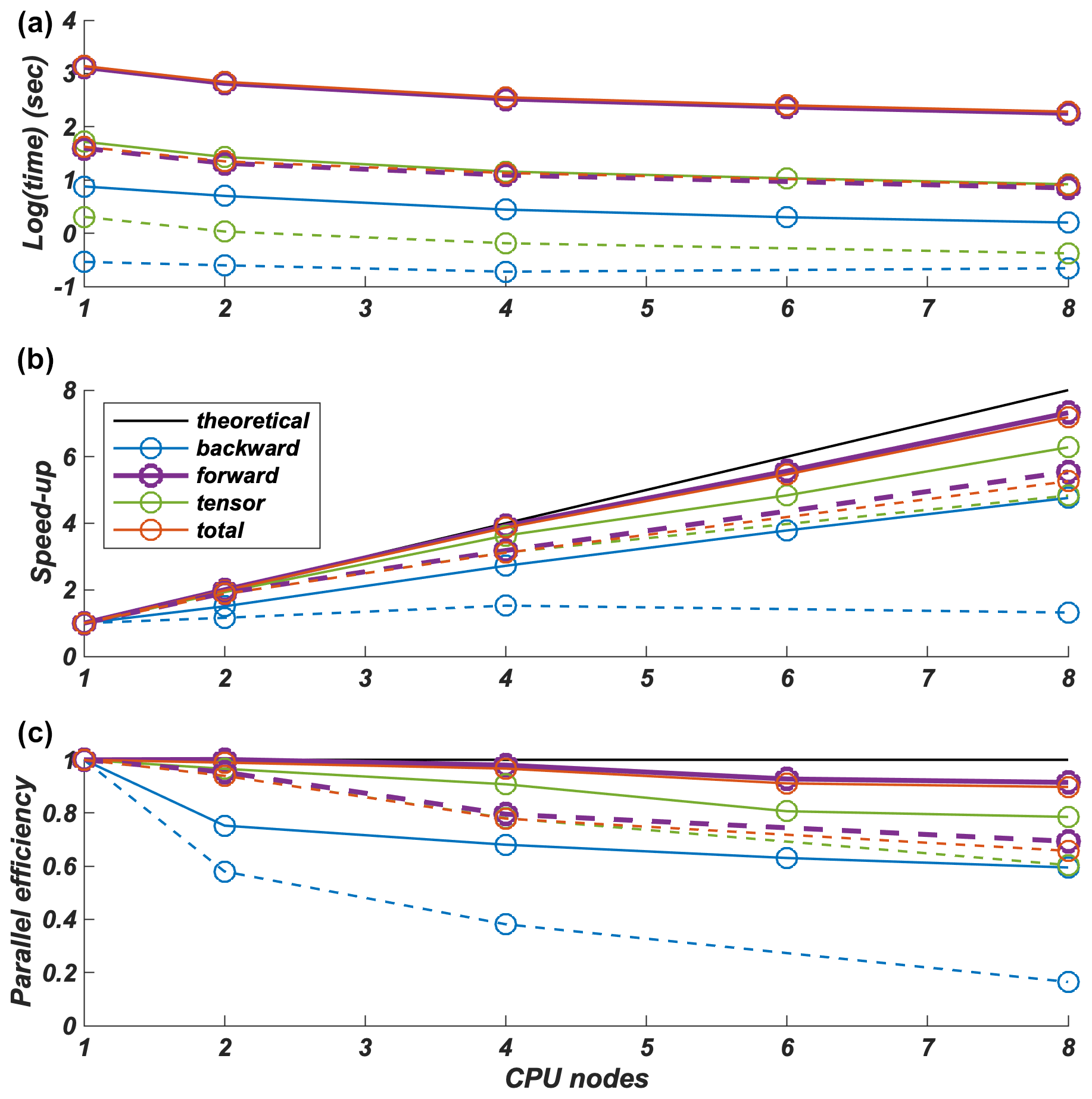
Figure 5 Runtime (a), speedup (b), and parallel efficiency (c) of D-REX_M for initial backward advection of aggregates (“backward”), forward advection and updating of the LPO and F tensor (“forward”), full elastic tensor computation and output file creation (“tensor”), and the entire run (“total”). Results are shown for two models included in the cookbooks: the 3Dspherical_global model (steady-state flow, 96 time steps, 1 327 606 aggregates, LPO computed only for 260 474 upper-mantle aggregates) and the 3Dspherical_sinkingslab model (dashed lines; time-dependent flow, 20 time steps, 38 509 aggregates, LPO computed for 25 177 aggregates in the upper mantle and 6587 in the upper mantle transition zone). Runs performed on an HPE Superdome Flex (eight CPUs, 28 cores Intel Xeon(R) PLATINUM 8180 @ 2.50 GHz) distributing the computational load over up to eight CPU nodes, each one working independently with 28 cores.

2.1.3 EXEV

EXEV includes routines to compute the extrinsic elastic and viscous anisotropy using effective medium theory modelling for a multi-component layered system (smoothed transversely isotropic long-wavelength equivalent, STILWE; Backus, 1962) or a two-component system with similar ellipsoidal inclusions in a uniform background matrix (differential effective medium, DEM; e.g. Mainprice, 1997).

The elastic tensor C due to SPO fabrics can either be estimated independently or, when using the DEM approach, superimposed on that obtained from the strain-induced LPO modelling. SPO fabrics that can be modelled are those related to rock- or grain-scale layering (e.g. Faccenda et al., 2019) or to the presence of preferentially aligned ellipsoidal inclusions (e.g. melt- and/or fluid-filled cracks). The user then needs to specify the following.

• For grain-scale layered fabrics, a dominant ultramafic or mafic lithology. In this case the mineral-phase proportions from the MMa-EoS lookup tables define the mixture for the STILWE model.

• For rock-scale layered fabrics, the relative abundance of the five available ultramafic–mafic lithologies (dunite, harzburgite, pyrolite, basalt, and pyroxenite) defining the mixture for the STILWE model.

• For matrix-inclusion fabrics, the elastic tensors of the two components and the inclusion's shape and volume fraction as required by the DEM modelling. The matrix elastic tensor can be replaced with that from the LPO modelling in order to estimate the combined effect of LPO and SPO fabrics.

The SPO fabrics can then be oriented at any angle relative to the principal finite-strain ellipsoid (FSE) axis or, in the case of cracks, the local principal stress obtained from the “present-day” (i.e. last) velocity field.

Summarising, SPO fabric modelling requires one or more of the following: F and/or C obtained from D-REX_M; P, T, and/or V and/or fluid and melt fraction fields for the “present-day” state of the geodynamic model. Consequently, this modelling is performed when post-processing the D-REX_M output with the software VIZTOMO (see Sect. 2.2.1).

The total or deviatoric component of the viscous tensor η due to SPO fabrics is estimated for two-phase systems with ellipsoidal weak or hard inclusions using the DEM theory, as well as the parameterisation of the viscous tensor evolution and orientation as a function of the cumulated deformation (F) obtained following de Montserrat et al. (2021). Indeed, most, if not all, mantle levels are composed of two main mineral phases that control both the elastic and viscous properties. The case of a multi-component layered medium is not considered because its viscous tensor can either be approximated with flat inclusions or more simply computed using the Voigt and Reuss averages of the layers' isotropic viscosity.

The first modelling phase requires running the subprogram DEMviscous to generate a database of viscous tensors for a range of inclusion shapes and volume fractions, as well as inclusion-matrix viscosity contrasts. The latter implies that the viscous moduli are dimensionless and can therefore be interpreted as scaling factors with respect to an isotropic effective viscosity of the bulk rock or most abundant mineral phase. Subsequently, the database can be exploited by large-scale geodynamic simulations to either (i) return the viscosity tensor η from a lookup table for every point of the computational domain, which can be superimposed on the isotropic effective viscosity computed from flow laws (coupled mechanical simulations), or (ii) estimate η (uncoupled mechanical simulation) and/or visualise its anisotropic viscous properties for the “present-day” state of the geodynamic model with the software VIZVISC (Sect. 2.2.2).

2.2 Visualisation of the mechanical properties and data formatting in preparation for seismological synthetics

2.2.1 VIZTOMO

VIZTOMO processes the D-REX_M output for the visualisation of the aggregates' elastic and deformational history properties. Estimation of extrinsic anisotropy effects via the EXEV routines is possible at this stage. The properties of the C and F tensors can either be determined at the position of the Lagrangian mantle aggregates or, in the case of the elastic properties and density, interpolated to a structured (tomographic) grid. In the latter case the grid can be saved in a format suitable for generating synthetic seismic datasets via the PSI_D package (see Sect. 2.3.2) or for 3D waveform simulations in SPECFEM (Komatitsch and Tromp, 1999).

Several properties of the elastic tensor C can be visualised:

• isotropic or ray-path-dependent velocity anomalies and anisotropic elastic properties of body waves (i.e. P-wave anisotropy and direction of maximum P-wave velocity, direction and magnitude of maximum S-wave splitting delay time, and S-wave radial and azimuthal anisotropy);

• reflection and/or transmission energies resulting from the whole range of P–S conversions occurring at discontinuities (useful for studies based on receiver function analysis);

• the fraction of the elastic tensor anisotropic component relative to the total and relative contributions of five different anisotropy classes (hexagonal, orthorhombic, tetragonal, monoclinic, triclinic) obtained through elastic tensor decomposition (Browaeys and Chevrot, 2004);

• the orientation of the hexagonal symmetry axis (already present in the original D-REX).

The deformation history stored in F can be visualised in terms of the FSE shape and orientation and/or length or orientation of its minimum and maximum semi-axes.

The different fields are saved in specific file formats which can be imported by the open-source ParaView software (Ahrens et al., 2005) for visualisation. Figs. 6–9 display some of these fields computed for different geodynamic models.

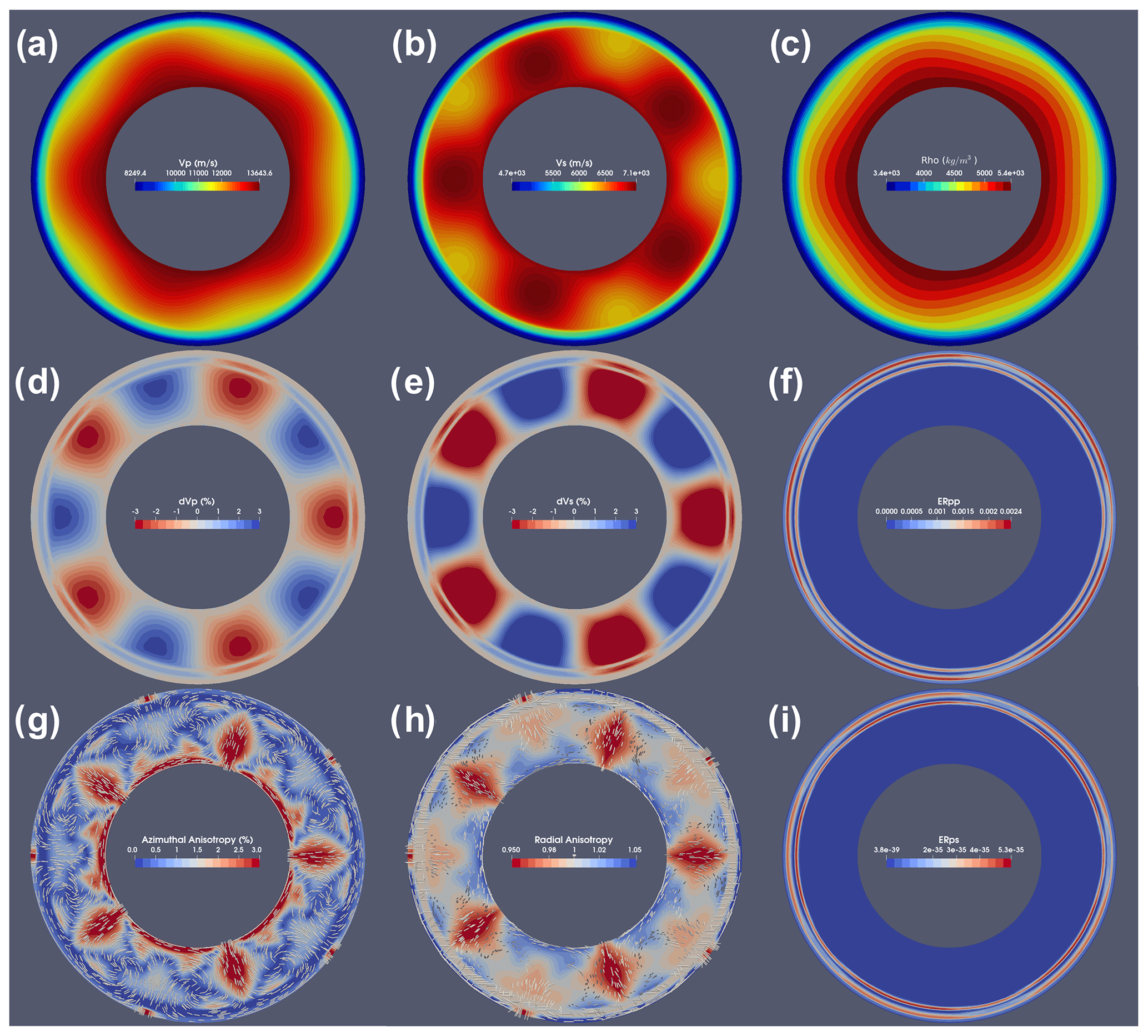
Figure 6 VIZTOMO output for the model 2Dpolar_convection available in the cookbooks. The steady-state 2D incompressible flow field in cylindrical coordinates is the result of the analytical solution shown in Sect. 9.3 of the software manual and coded in the MATLAB script cookbooks/2Dpolar_convection/polarcell.m. (a, b) Isotropic V_p and V_s (m s⁻¹), (c) density, (d, e) isotropic P- and S-wave anomalies, (g) azimuthal anisotropy and FSE semi-axis (white bars), (h) radial anisotropy and TTI axis (white bars), and (f, i) P–P and P–S reflection energy for waves propagating upward.

Figure 7 VIZTOMO output for a 3D model of oceanic plate subduction and roll-back in spherical coordinates. The time-dependent flow field has been computed with the software I3MG modified to account for spherical coordinates (see Faccenda and VanderBeek, 2023). Fabrics are computed with D-REX_M for only upper-mantle aggregates. A fossil A-type olivine fabric with the fast axis parallel to plate motion and computed with D-REX_S is initially defined within the oceanic plate volume. The colour scale indicates radial anisotropy in the upper mantle, and the white bars indicate the SKS splitting computed with SKS-SPLIT. The volume in green encloses material with a +2 % P-wave anomaly (i.e. the oceanic plate). Note the apparently thicker slab portion around the 410 km depth discontinuity due to the upwelling of the olivine–spinel phase transition. The model domain extends from 0–1000 km along the radial direction, 85–115° along longitude, and 70–90° along colatitude.

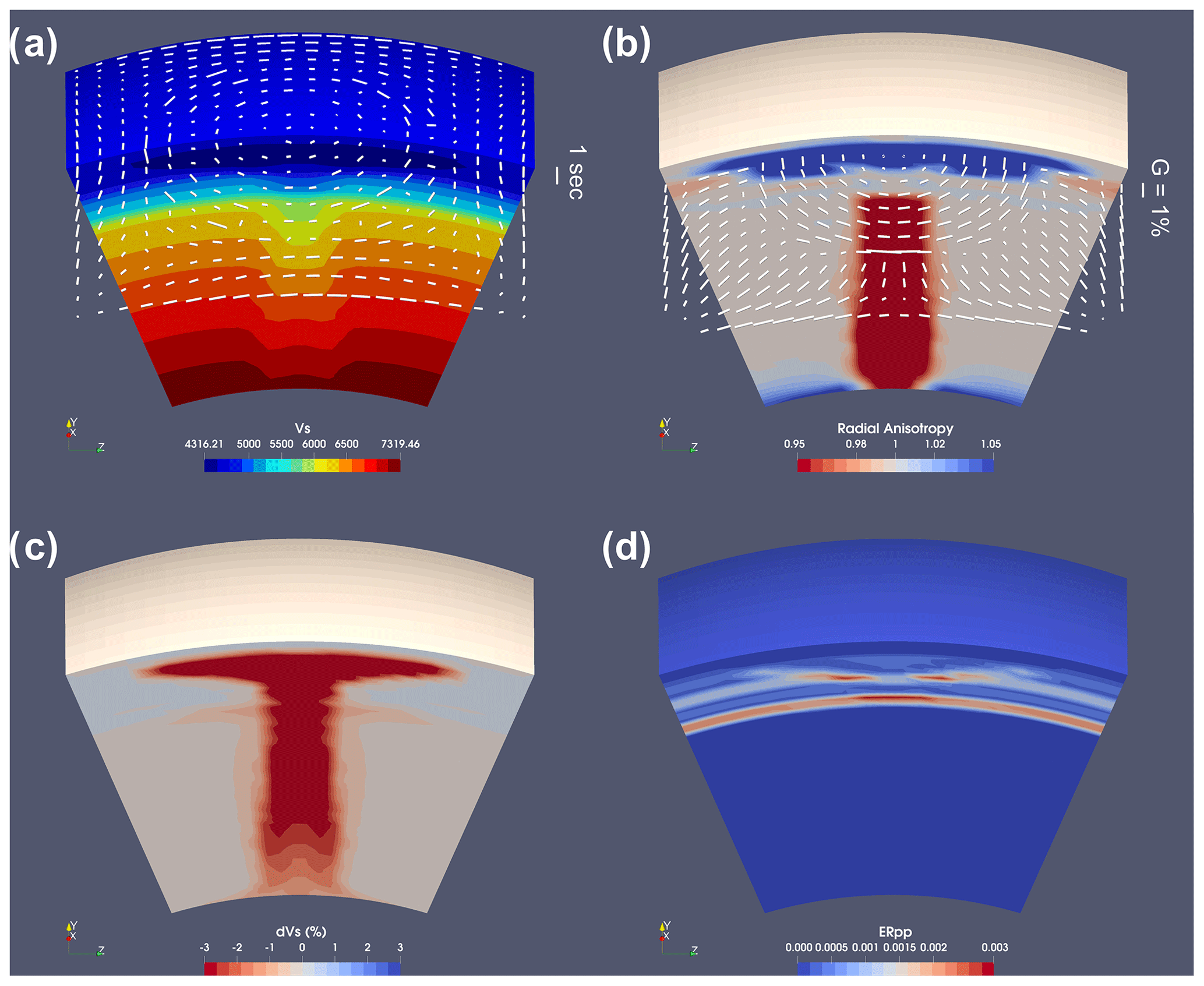
Figure 8 VIZTOMO output for an upwelling plume toy model in spherical coordinates. The time-dependent flow field has been computed with the software I3MG modified to account for spherical coordinates (see Faccenda and VanderBeek, 2023). (a) Absolute V_s (m s⁻¹) and SKS splitting computed with SKS-SPLIT (white bars), (b) radial anisotropy (colour scale) and azimuthal anisotropy at 200 km depth (white bars), (c) isotropic V_s anomaly, and (d) P–P reflection energy for a wave propagating upward. The model domain extends from 0–2900 km along the radial direction, 70–110° along longitude, and 70–110° along colatitude.

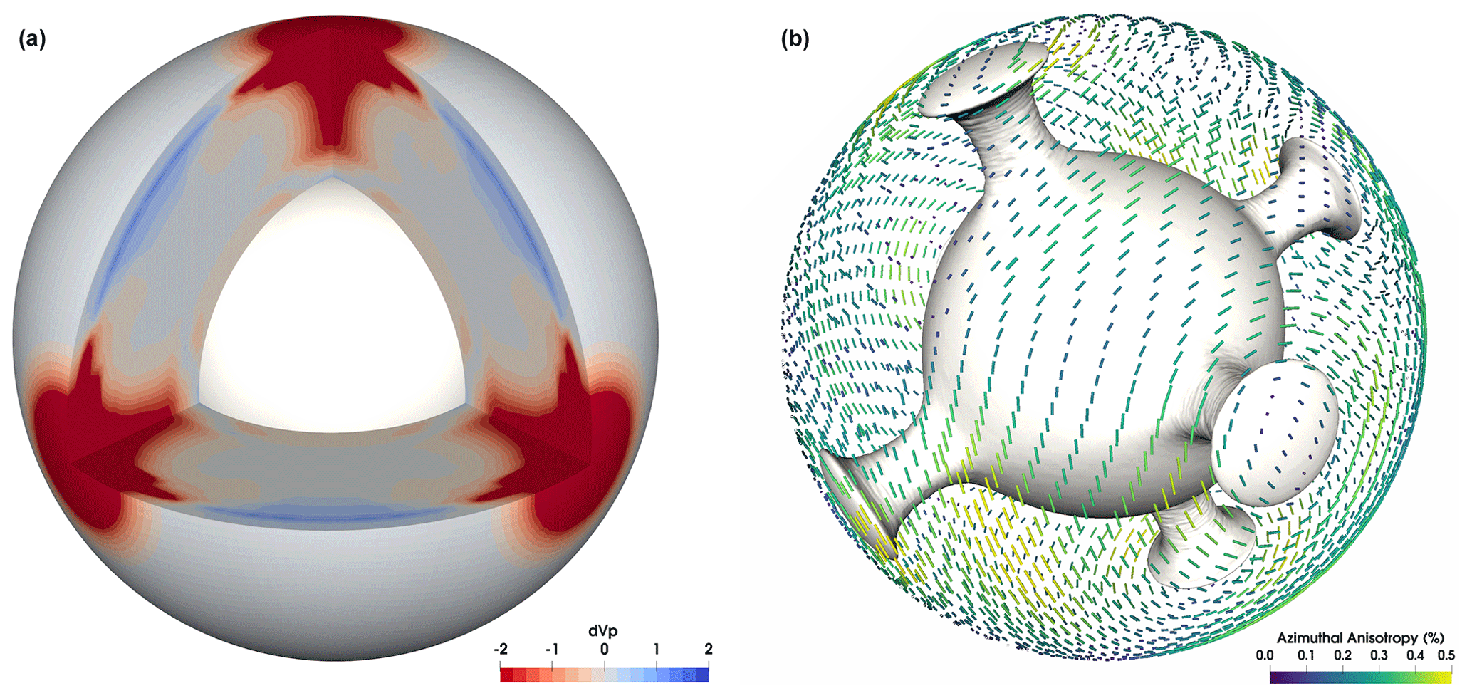
Figure 9 VIZTOMO output for the model 3Dspherical_global available in the cookbooks. The time-dependent flow field has been computed with the software I3MG modified to account for 3D global spherical coordinates using Yin–Yang grids (Kageyama and Sato, 2004). Isotropic P-wave anomaly (a) and azimuthal anisotropy at 200 km depth (b). The grey surface encloses material 0.1 dimensionless units hotter than the average temperature at any depth.

2.2.2 VIZVISC

VIZVISC processes the D-REX_M output for the visualisation of the aggregate properties such as the viscous anisotropy and related deformational history (in terms of the FSE) in ParaView. The deviation from isotropy is evaluated by computing the radial and azimuthal components of viscous anisotropy in a similar way as for the elastic tensor. More in detail, radial viscous anisotropy is defined as $\mathit{\xi }=N/L$, while azimuthal viscous anisotropy is defined by the magnitude $G=\sqrt{G_{\mathrm{c}}^{\mathrm{2}}+G_{\mathrm{s}}^{\mathrm{2}}}$ and azimuth $\mathit{\varphi }={\tan }^{-\mathrm{1}}\left(G_{\mathrm{s}}{G}_{\mathrm{c}}\right)$, where $N=\mathrm{1}/\mathrm{8}({\mathit{\eta }}_{\mathrm{11}}+{\mathit{\eta }}_{\mathrm{22}})-\mathrm{1}/\mathrm{4}{\mathit{\eta }}_{\mathrm{12}}+\mathrm{1}/\mathrm{2}{\mathit{\eta }}_{\mathrm{66}}$, $L=\mathrm{1}/\mathrm{2}({\mathit{\eta }}_{\mathrm{44}}+{\mathit{\eta }}_{\mathrm{55}})$, $G_{\mathrm{c}}=\mathrm{1}/\mathrm{2}({\mathit{\eta }}_{\mathrm{55}}-{\mathit{\eta }}_{\mathrm{44}})$, and G_s=η₄₅. Radial anisotropy and azimuthal viscous anisotropy are evaluated in the FSE (and thus inclusions) reference frame, whereby the minor semi-axis is oriented along the vertical direction, and the intermediate and major semi-axes are in the horizontal plane. As such, radial anisotropy is always ≥1. Figure 10 displays some of these fields computed for a 2D steady-state model of mantle convection with periodic upwellings and downwellings.

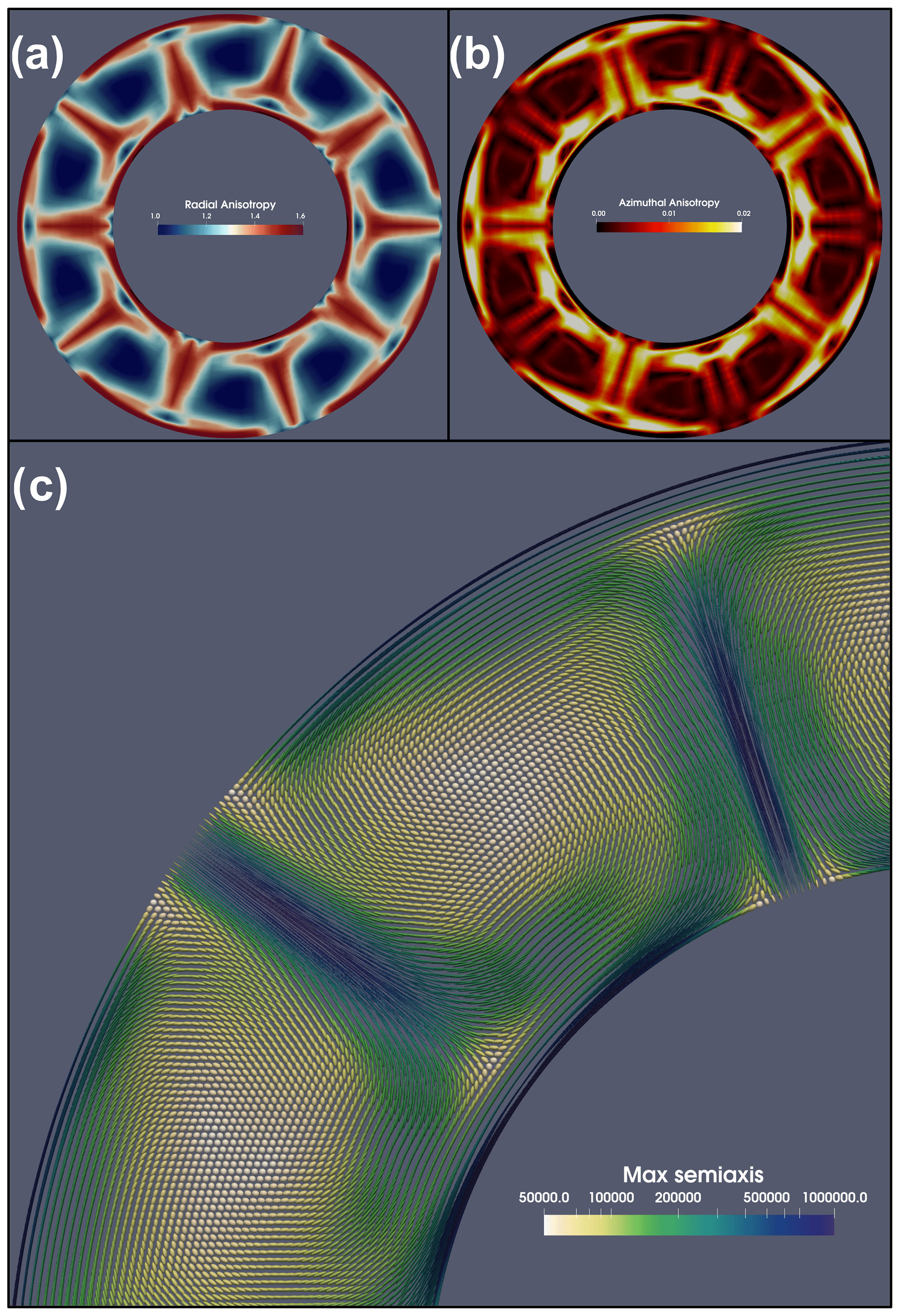
Figure 10 VIZVISC output for the model 2Dpolar_convection available in the cookbooks. The steady-state 2D incompressible flow field in cylindrical coordinates is the result of the analytical solution shown in Sect. 9.3 of the software manual and coded in the MATLAB script cookbooks/2Dpolar_convection/polarcell.m. (a) Radial viscous anisotropy, (b) azimuthal viscous anisotropy, and (c) FSE shape coloured by the length of its major semi-axis upscaled by a factor of 50 km.

2.3 Seismic forward and inverse modelling

2.3.1 SKS-SPLIT

SKS-SPLIT estimates the SKS splitting at a grid of virtual seismic stations placed at the top of the D-REX_M model as a function of the back azimuth using the Fortran routines included in FSTRACK (Schulte-Pelkum and Blackman, 2003; Becker et al., 2006). These routines use the reflectivity method (for details, see Booth and Crampin, 1983; Chapman and Shearer, 1989) to compute synthetic seismograms through layered anisotropic media traversed by an incident plane wave (5° for typical SKS arrivals) over a range of frequencies (0–25 Hz). Bandpass filters from 0.1 to 0.3 Hz are then applied to construct synthetic seismograms in the SKS band (3.3 to 10 s). Successively, the splitting is determined with the cross-correlation method of Menke and Levin (2003). The routines have been adapted to load the D-REX_M output, stack the elastic tensors and densities in an upper-mantle rock column beneath each virtual seismic station (Faccenda and Capitanio, 2013), and run in parallel using MPI. The averaged fast azimuth scaled by the delay time can then be visualised in ParaView as shown in Figs. 7 and 8a.

2.3.2 PSI

PSI (Platform for Seismic Imaging) is a Julia package for performing tomographic inversion of both real and synthetic seismic datasets. In the context of the ECOMAN software, it is a useful tool for exploring how features in high-resolution geodynamic simulations are mapped into lower-resolution seismic tomography models; this is a critical step if one aims to evaluate geodynamic results against existing tomographic images.

PSI can be used to forward-model P and S travel times, splitting intensity (Chevrot, 2000), and shear wave splitting parameters (i.e. the fast-polarisation azimuth and the delay time between the fast- and slow-polarised waveforms). Forward modelling of these seismic observables is supported for three different model parameterisations: (1) isotropic P- and S-wave speeds, (2) hexagonally anisotropic media defined by the five Thomsen parameters and the azimuth and elevation of the symmetry axis, and (3) fully anisotropic models defined by the density-normalised 21-component elastic tensor which can be generated from D-REX_M + VIZTOMO (Sect. 2.1.2 and 2.2.1). Seismic phase velocities are computed following Thomsen (1986) for hexagonally anisotropic models, while the Christoffel equations are solved when the elastic tensor parameterisation is used. Anisotropic travel times and splitting intensities for arbitrarily polarised S-waves are computed following VanderBeek et al. (2023) using a long-wavelength approximation in which the accumulated delay time between fast- and slow-polarised qS waves is less than their dominant period. Lastly, splitting parameters are predicted using the matrix propagation method of Rumpker and Silver (1998). In this initial release of PSI, all predictions are made via integration along ray paths traced through a user-defined 1D reference velocity model using the TauP Toolkit (Crotwell et al., 1999). The 3D model properties are subsequently interpolated to these paths before computing the seismic observables. We anticipate releasing an update to the package that includes both 3D anisotropic ray tracing and finite-frequency kernels that are currently under development.

Travel time and splitting intensity datasets can be inverted individually and jointly either for isotropic (V_p and V_s) or hexagonally anisotropic model parameters. Hexagonal anisotropy is defined by up to five free parameters, the isotropic (1) P and (2) S velocity, (3) anisotropic magnitude, and the (4) azimuth and (5) elevation of the hexagonal symmetry axis. Only a single anisotropic magnitude parameter is required because the strength of P and S anisotropy is strongly correlated (e.g. Becker et al., 2006). Consequently, the ratios between the three Thomsen parameters (ε, δ, γ; Thomsen, 1986) and the inverted anisotropic magnitude parameter must be chosen a priori and can be spatially variable. Source and receiver statics for each observation and seismic phase type may also be included as free parameters. The tomographic model is obtained by iteratively solving a system of linearised equations relating the perturbations in the inversion parameters to the data residuals augmented with damping and smoothing constraints. The solution is obtained via the LSQR algorithm (Paige and Saunders, 1982). Full details on the tomographic method can be found in VanderBeek and Faccenda (2021) and VanderBeek et al. (2023). The final tomographic solution is written to a VTK file to be visualised in ParaView. Tomographic inversions can be run from a workstation. For the problem shown in Fig. 11 consisting of 12 320 observations and 415 044 free parameters, solutions can be obtained within ∼10 min (less for isotropic inversions) using six cores and 1.8 GB peak RAM.

Figure 11 Synthetic tomography results obtained from PSI for the model shown in Fig. 7. (a) Target anisotropic model generated from VIZTOMO. (b) Recovered anisotropic model obtained by inverting synthetic teleseismic P and S (relative) delay times computed from the model in (a). In both panels, the isotropic S-wave velocity perturbations are computed with respect to the far-field 1D velocity profile. Quivers parallel the hexagonal symmetry axis and are scaled and coloured by the anisotropic strength. The top surface shown is located at 200 km depth, while the full model extends from 0–1000 km along the radial direction, 85–115° along longitude, and 0–20° along latitude.

The PSI inversion methodology has been tested on synthetic models of oceanic plate subduction, intra-oceanic upwelling plume, spreading oceanic ridge, and central–eastern Mediterranean subduction (VanderBeek and Faccenda, 2021; Lo Bue et al., 2021, 2022; VanderBeek et al., 2023; Faccenda and VanderBeek, 2023) and applied to the isotropic and anisotropic imaging of the central Mediterranean (Rappisi et al., 2022) and of the Mt. Etna volcanic field (Lo Bue et al., 2024). In Fig. 11, we illustrate results obtained from a synthetic inversion of direct teleseismic P- and S-wave relative travel times computed through the subduction zone shown in Fig. 7. Synthetic data were computed using the full 21-component elastic tensor, while the inversion was performed for the best-fit hexagonal anisotropic parameters. We considered an array of 770 receivers extending from ±7.5° in longitude and ±11.5° in latitude (∼75 km spacing) that recorded 16 events: 8 at 50° and another 8 at 80° from the origin of the subduction zone model and equally distributed in the back azimuth. This example is included in the PSI package.

3 Discussion

3.1 Software advantages

When compared to other similar software, ECOMAN (i) is a more versatile package suitable for any geodynamic simulations (2D and 3D; Cartesian and polar coordinate systems; regional and global settings); (ii) allows for the possibility to account for the time-dependent deformational history of the mantle (which is usually not steady-state, especially close to plate boundaries and hotspot settings); (iii) computes the strain-induced fabric and elastic tensor of different mantle layers (i.e. not only the upper mantle); (iv) includes effective medium theories (STILWE, DEM) and a parameterisation of the fabric evolution of two-phase composites to predict elastic and viscous extrinsic anisotropy; (v) generates realistic grid structure distributions of mantle elastic properties to be used for forward and inverse seismological modelling (e.g. PSI, SPECFEM3D); and (vi) performs synthetic seismic inversions (e.g. P- and S-wave travel time tomographies, S-wave splitting intensities) within the computational domain, which facilitates the comparison with other tomographic models and the estimation of apparent anomalies (artefacts) due to, for example, unaccounted for elastic anisotropy (Bezada et al., 2016; VanderBeek and Faccenda, 2021; VanderBeek et al., 2023) and/or regularisation.

3.2 Software (real or potential) current limitations

D-REX_S and D-REX_M compute the strain-induced LPO for the most abundant and highly anisotropic mineral phases, while assuming random orientation for several secondary phases that instead could contribute substantially to the aggregate anisotropic properties. For example, cubic ferropericlase is relatively abundant (<20 %) and becomes highly anisotropic in the lower half of the lower mantle (Avs = 30 %–50 %) such that it could dominate seismic anisotropy at these depths (Marquardt et al., 2009). Davemaoite (Ca-perovskite) is also a highly anisotropic mineral with cubic symmetry (Avs = 25 %–15 %; Kawai and Tsuchiya, 2015) but its model abundance is quite low (<10 %). Recently, micro-mechanical simulations of strain-induced LPO in aggregates with a pyrolite mantle composition have shown that the bulk aggregate seismic anisotropy is controlled by bridgmanite and post-perovskite, while the cubic secondary phases appear to only slightly reduce the amplitude of anisotropy (Chandler et al., 2021). The latter effect can thus be well approximated by randomising the orientation of the cubic phases as assumed here.

A main limitation of ECOMAN is that it does not yet include the modelling of viscous anisotropy due to the intrinsic mechanical anisotropy of crystals. Tommasi et al. (2009) used VPSC simulations to show that olivine CPO in the lithosphere can control the reactivation of fossil faults misoriented with respect to the stress field. Király et al. (2020) employed the modified director method (MDM) and estimated up to 1 order of magnitude of intrinsic viscous anisotropy in olivine aggregates, which can control the kinematics and dynamics of tectonic plates. Both the VPSC and MDM approaches are computationally expensive and appear to be prohibitive for the number of mantle aggregates required to discretise the mantle domain of large-scale 3D simulations. An alternative approach which minimises the computational time is therefore desired.

Fraters and Billen (2021) released a version of the D-REX model that is embedded into the ASPECT geodynamic modelling software (Bangerth et al., 2020) and that takes into account changes in olivine fabric as a function of the water content and deviatoric stress (Karato et al., 2008). Although at present D-REX_M only allows the definition of a single olivine fabric per run, changes in crystal fabrics can be easily implemented in the future by loading the water content and deviatoric stress field from the geodynamic models and by parameterising the boundaries of the olivine fabric domains.

Tape and Tape (2024) recently reformulated the elastic decomposition method proposed by Browaeys and Chevrot (2004) that they argued is not entirely accurate. Although this will only affect the visualisation of the tensor components as performed by D-REX_S and VIZTOMO, it is planned to replace the existing elastic tensor decomposition methodology with the one proposed by Tape and Tape (2024).

A minor limitation is that the different code modules are based on different programming languages (Fortran, Julia), libraries (OpenMP, MPI, HDF5), and software (MATLAB, ParaView), whose installation on local devices might discourage potential users. There are a few main reasons for this. First of all, the original D-REX software was written in Fortran, and thus its modification in D-REX_S and D-REX_M software was more straightforward by maintaining the same programming language. Fortran has high performance standards on HPC clusters that are often if not always higher than other interpreted programming languages (e.g. MATLAB or Python). Given the large-scale computational power needed for the D-REX_M simulations, especially those with hundreds of thousands or millions of crystal aggregates, and considering that the required compilers and libraries are routinely installed in most (if not all) HPC clusters, the usage of the ECOMAN's Fortran-based applications in high-performance environments is warranted. In contrast, the visualisation of the Fortran-based applications' output in MATLAB and ParaView can be performed on local devices. In particular, the MTEX software is a MATLAB toolbox for visualisation of the LPO and elastic tensor pole figures which should be downloaded (https://mtex-toolbox.github.io/download, last access: 1 October 2024) and installed along with MATLAB only when using D_REX_S. Seismic forward and inverse modelling with PSI can be performed on either an HPC cluster or local devices upon installation of the Julia package. Julia was chosen because it is an open-source and high-level language that offers a number of performance benefits over other popular scientific computing languages such as Python and MATLAB. It is important to stress that for any of these applications the user only needs to modify input text files, and thus no particular prerequisite or computational skill is required.

Finally, running D-REX_M requires allocating ∼160 GB of memory per million crystal aggregates with 1000×2 crystals each. This potential problem can be addressed by distributing the computational and memory load over several nodes, which is possible thanks to the hybrid MPI and OpenMP parallelisation scheme.

4 Conclusions and outlook

ECOMAN is an open-source software package for estimating strain- and stress-induced fabrics in mantle aggregates, their mechanical properties, and how mechanical anisotropy affects the geodynamic evolution and seismic imaging of the Earth's interior. Programs included in ECOMAN are portable across different HPC and local device systems (provided the Julia package and Fortran compilers are available) and are applicable to any 2D–3D geodynamic simulation. Computationally expensive programs such as D-REX_M are parallelised, offering a nearly perfect scaling with an increasing number of cores. As a result, the strain-induced fabrics of millions of mantle aggregates can now be estimated with a reasonable quantity of time and computational resources.

As ongoing developments, we are seeking to include in ECOMAN micro-mechanical modelling methods that are capable of estimating the strain-induced LPO and/or the intrinsic viscous anisotropy at computational speeds that are orders of magnitude faster than current ones. For instance, Ribe et al. (2019) proposed an analytical finite-strain parameterisation for texture evolution in deforming olivine polycrystals that is ≈10⁷ times faster than full homogenisation approaches such as the second-order self-consistent model. When implemented in ECOMAN, preliminary tests indicate that this new method outperforms D-REX by 1–2 orders of magnitude (Ribe et al., 2023).

In addition, in the near future the PSI software will be updated to include trans-dimensional Bayesian Monte Carlo sampling methods that, in contrast to deterministic approaches, address the consequences of underdetermination in seismic imaging by constraining the uncertainty (Del Piccolo et al., 2024). Isotropic and anisotropic seismic imaging with PSI is currently feasible using body wave information such as travel times and S-wave splitting intensity. However, when local deep seismicity is absent, as is the case in warm subduction zones or at spreading ridges and intraplate settings, the retrieved isotropic and anisotropic mantle structures are only partially recovered and often affected by smearing (e.g. Faccenda and VanderBeek, 2023). Consequently, we are planning to complement body wave information with surface wave data to improve the seismic ray coverage and the resolving power of tomographic models. Lastly, to improve the prediction of seismic observables, 3D anisotropic ray tracing and finite-frequency kernels are planned for a future release.

Appendix A: D-REX model vs. analytical solution

We compare the numerical solution of the D-REX model included in D-REX_S and D-REX_M with the analytical solution provided by Fraters and Billen (2021, Supplement) for a test with an upper-mantle aggregate ($Ol:Ens=\mathrm{50}:\mathrm{50})$ composed of five crystals for each phase, $M^{*}=\mathrm{50}$, χ=0.3, and $\mathrm{nCRSS}=(\mathrm{1},\mathrm{2},\mathrm{3},\mathrm{\infty })$ for the four olivine slip systems [100](010), [100](001), [001](010), and [001](100) (Table A1). For the first crystal, the time derivative of the cosine direction matrix (CDM) is $\frac{\mathit{\delta }{a}_{ij}^{\mathrm{v}}}{\mathit{\delta }t}=\mathrm{0}$ and the vorticity matrix is ${\stackrel{\mathrm{‾}}{\mathit{\omega }}}_{ij}^{\mathrm{v}}={\mathit{\epsilon }}_{jki}{\mathit{\omega }}_k^v=\mathrm{0}$, while for the other four crystals

$$\begin{array}{}\text{(A1)}& {\displaystyle \frac{\mathit{\delta }{a}_{ij}^{\mathrm{v}}}{\mathit{\delta }t}}=\left[\begin{array}{ccc}-\mathrm{0.0040153}& -\mathrm{0.0010038}& \mathrm{0.0020076}\\ -\mathrm{0.0085325}& -\mathrm{0.0010038}& \mathrm{0.0065249}\\ -\mathrm{0.0130497}& -\mathrm{0.0010038}& \mathrm{0.0110421},\end{array}\right.\end{array}$$

with a maximum error of $\mathrm{3.1}\times {\mathrm{10}}^{-\mathrm{3}}$ %, which we attribute to truncation errors, and

$$\begin{array}{}\text{(A2)}& {\stackrel{\mathrm{‾}}{\mathit{\omega }}}_{ij}^{\mathrm{v}}=\left[\begin{array}{rrr}\mathrm{0}& \mathrm{0.005019}& \mathrm{0.010038}\\ -\mathrm{0.005019}& \mathrm{0}& \mathrm{0.005019}\\ -\mathrm{0.010038}& -\mathrm{0.005019}& \mathrm{0}.\end{array}\right].\end{array}$$

The changes in volume fractions are $\frac{\mathit{\delta }{f}_{\mathrm{m}}^{\mathrm{v}}}{\mathit{\delta }t}=\mathrm{0.630116863029}$ for grain 1 and $\frac{\mathit{\delta }{f}_{\mathrm{m}}^{\mathrm{v}}}{\mathit{\delta }t}=-\mathrm{0.157529215757}$ for the other four crystals, resulting in a misfit of $\mathrm{6.5244}\times {\mathrm{10}}^{-\mathrm{4}}$ % relative to the analytical solution.

We provide the D-REX_S_test program for reproducing this simple test in the Supplement.

Table A1 Available slip systems of abundant anisotropic mantle phases present in D-REX_S and D-REX_M.

Appendix B: Aggregate elastic stiffness tensor

At any P–T condition, the single-crystal elastic moduli $C_{ij}^{\mathrm{m}}$ are (in Voigt notation)

$$\begin{array}{}\text{(B1)}& \begin{array}{rl}{C}_{ij}^{\mathrm{m}}(P,T)& =C_{ij}^{\mathrm{m}}\left(P_{\mathrm{0}},T_{\mathrm{0}}\right)+\partial C_{ij}^{\mathrm{m}}/\partial P\cdot \mathrm{\Delta }P+\mathrm{0.5}\\ & \cdot {\partial }^{\mathrm{2}}{C}_{ij}^{\mathrm{m}}/\partial P^{\mathrm{2}}\cdot \mathrm{\Delta }{P}^{\mathrm{2}}+\partial C_{ij}^{\mathrm{m}}/\partial T\cdot \mathrm{\Delta }T\\ & +{\partial }^{\mathrm{2}}{C}_{ij}^{\mathrm{m}}/\partial P\partial T\cdot \mathrm{\Delta }P\mathrm{\Delta }T,\end{array}\end{array}$$

where the partial derivatives are listed in Table B2 and ΔP and ΔT are deviations from the room conditions ($P_{\mathrm{0}}={\mathrm{10}}^{-\mathrm{4}}$ GPa, T₀=298 K; Mainprice, 2007). The compliance tensor is the inverse of the stiffness tensor, i.e. ${\mathbf{S}}^{\mathrm{m}}={\mathbf{C}}^{{\mathrm{m}}^{-\mathrm{1}}}$. These tensors can be rotated as

$$\begin{array}{}\text{(B2)}& {\displaystyle }& {\displaystyle }{C}_{ijkl}^{\mathrm{v}}=a_{ip}{a}_{jq}{a}_{kr}{a}_{ls}{C}_{pqrs}^{\mathrm{m}},\text{(B3)}& {\displaystyle }& {\displaystyle }{S}_{ijkl}^{\mathrm{v}}=a_{ip}{a}_{jq}{a}_{kr}{a}_{ls}{S}_{pqrs}^{\mathrm{m}},\end{array}$$

where a is the CDM defining the crystal orientation with respect to the external reference frame. The stiffness and compliance tensors of the crystal aggregate (i.e. rock) are then obtained by arithmetic averaging:

$$\begin{array}{}\text{(B4)}& {\displaystyle }& {\displaystyle }{\mathbf{C}}^{\mathrm{r}}=\sum _{m=\mathrm{1}}^M{X}_{\mathrm{m}}\sum _{v=\mathrm{1}}^N{X}_{\mathrm{v}}{\mathbf{C}}^{\mathrm{v}},\text{(B5)}& {\displaystyle }& {\displaystyle }{\mathbf{S}}^{\mathrm{r}}=\sum _{m=\mathrm{1}}^M{X}_{\mathrm{m}}\sum _{v=\mathrm{1}}^N{X}_{\mathrm{v}}{\mathbf{S}}^{\mathrm{v}},\end{array}$$

where M=2 is the number of minerals in the two-phase mantle aggregates modelled in D-REX_M and D-REX_S, X_m their relative abundance, N the number of crystals of each phase, and X_v the normalised crystal volume fraction ($\sum _{v=\mathrm{1}}^N{X}_{\mathrm{v}}=\mathrm{1}$). C^r and (S^r)⁻¹ correspond to the Voigt and Reuss average stiffness tensor of the rock, i.e. ${\mathbf{C}}_{\mathrm{Voigt}}^{\mathrm{r}}$ and ${\mathbf{C}}_{\mathrm{Reuss}}^{\mathrm{r}}$. More in general, the average stiffness tensor resulting from the linear combination of the two end members is found as

$$\begin{array}{}\text{(B6)}& {\stackrel{\mathrm{‾}}{\mathbf{C}}}^{\mathrm{r}}=X_{\mathrm{Voigt}}{\mathbf{C}}_{\mathrm{Voigt}}^{\mathrm{r}}+\left(\mathrm{1}-X_{\mathrm{Voigt}}\right){\mathbf{C}}_{\mathrm{Reuss}}^{\mathrm{r}},\end{array}$$

where X_Voigt is a free parameter defining the fraction of ${\mathbf{C}}_{\mathrm{Voigt}}^{\mathrm{r}}$ relative to ${\mathbf{C}}_{\mathrm{Reuss}}^{\mathrm{r}}$. It is clear that the Hill average stiffness tensor ${\mathbf{C}}_{\mathrm{Hill}}^{\mathrm{r}}$ is obtained when X_Voigt=0.5.

The isotropic component of the average stiffness tensor ${\stackrel{\mathrm{‾}}{\mathbf{C}}}_{\mathrm{ISO}}^{\mathrm{r}}$ can be assembled as ${\stackrel{\mathrm{‾}}{C}}_{\mathrm{ISO}\mathrm{\_}\mathrm{11}}^{\mathrm{r}}={\stackrel{\mathrm{‾}}{C}}_{\mathrm{ISO}\mathrm{\_}\mathrm{22}}^{\mathrm{r}}={\stackrel{\mathrm{‾}}{C}}_{\mathrm{ISO}\mathrm{\_}\mathrm{33}}^{\mathrm{r}}=K+\frac{\mathrm{4}}{\mathrm{3}}G$, ${\stackrel{\mathrm{‾}}{C}}_{\mathrm{ISO}\mathrm{\_}\mathrm{12}}^{\mathrm{r}}={\stackrel{\mathrm{‾}}{C}}_{\mathrm{ISO}\mathrm{\_}\mathrm{13}}^{\mathrm{r}}={\stackrel{\mathrm{‾}}{C}}_{\mathrm{ISO}\mathrm{\_}\mathrm{23}}^{\mathrm{r}}=K-\frac{\mathrm{2}}{\mathrm{3}}G$, and ${\stackrel{\mathrm{‾}}{C}}_{\mathrm{ISO}\mathrm{\_}\mathrm{44}}^{\mathrm{r}}={\stackrel{\mathrm{‾}}{C}}_{\mathrm{ISO}\mathrm{\_}\mathrm{55}}^{\mathrm{r}}={\stackrel{\mathrm{‾}}{C}}_{\mathrm{ISO}\mathrm{\_}\mathrm{66}}^{\mathrm{r}}=G$, knowing that:=

$$\begin{array}{}\text{(B7)}& {\displaystyle }& {\displaystyle }K={\displaystyle \frac{\left[\left({\stackrel{\mathrm{‾}}{C}}_{\mathrm{11}}^{\mathrm{r}}+{\stackrel{\mathrm{‾}}{C}}_{\mathrm{22}}^{\mathrm{r}}+{\stackrel{\mathrm{‾}}{C}}_{\mathrm{33}}^{\mathrm{r}}\right)+\mathrm{2}\left({\stackrel{\mathrm{‾}}{C}}_{\mathrm{12}}^{\mathrm{r}}+{\stackrel{\mathrm{‾}}{C}}_{\mathrm{13}}^{\mathrm{r}}+{\stackrel{\mathrm{‾}}{C}}_{\mathrm{23}}^{\mathrm{r}}\right)\right]}{\mathrm{9}}},\text{(B8)}& {\displaystyle }& {\displaystyle }G={\displaystyle \frac{\left[\left({\stackrel{\mathrm{‾}}{C}}_{\mathrm{11}}^{\mathrm{r}}+{\stackrel{\mathrm{‾}}{C}}_{\mathrm{22}}^{\mathrm{r}}+{\stackrel{\mathrm{‾}}{C}}_{\mathrm{33}}^{\mathrm{r}}\right)-\left({\stackrel{\mathrm{‾}}{C}}_{\mathrm{12}}^{\mathrm{r}}+{\stackrel{\mathrm{‾}}{C}}_{\mathrm{13}}^{\mathrm{r}}+{\stackrel{\mathrm{‾}}{C}}_{\mathrm{23}}^{\mathrm{r}}\right)+\mathrm{3}\left({\stackrel{\mathrm{‾}}{C}}_{\mathrm{44}}^{\mathrm{r}}+{\stackrel{\mathrm{‾}}{C}}_{\mathrm{55}}^{\mathrm{r}}+{\stackrel{\mathrm{‾}}{C}}_{\mathrm{66}}^{\mathrm{r}}\right)\right]}{\mathrm{15}}}.\end{array}$$

The isotropic component of the aggregate stiffness tensor ${\stackrel{\mathrm{‾}}{\mathbf{C}}}_{\mathrm{ISO}}^{\mathrm{r}}$ is then replaced with the isotropic stiffness tensor ${\mathbf{C}}_{\mathrm{ISO}}^{\mathrm{MMA}\mathrm{EoS}}$ obtained using the bulk and shear moduli from the lookup tables computed with the MMA_EoS software (Chust et al., 2017) as

$$\begin{array}{}\text{(B9)}& {\stackrel{\mathrm{‾}}{\mathbf{C}}}_{\mathrm{MMA}\mathrm{\_}\mathrm{EoS}}^{\mathrm{r}}={\stackrel{\mathrm{‾}}{\mathbf{C}}}^{\mathrm{r}}+{\mathbf{C}}_{\mathrm{ISO}}^{\mathrm{MMA}\mathrm{\_}\mathrm{EoS}}-{\stackrel{\mathrm{‾}}{\mathbf{C}}}_{\mathrm{ISO}}^{\mathrm{r}}.\end{array}$$

Table B1 Composition (in mol %) used in MMA_EoS to compute lookup tables for different mantle and basalt composition.

^* (1) Kelemen and Ghiorso (1986); (2) Chemia et al. (2015); (3) Workman and Hart (2005); (4) Hirschmann et al. (2003).

Table B2 Elastic moduli (GPa) and their P–T derivatives of the mineral phases present in ECOMAN. Temperature derivatives are scaled by 10² GPa K⁻¹ and cross-derivatives by 10⁻³ K⁻¹.

^* (1) Isaak (1992); (2) Zha et al. (1998); (3) Chai et al. (1992); (4) Jackson et al. (2007); (5) Zha et al. (1997); (6) Zhou et al. (2022); (7) Sinogeikin et al. (2003); (8) Chai and Brown (1997); (9) Sinogeikin and Bass (2002); (10) Wentzcovitch et al. (2004). Derivatives at 100 GPa and 300 K: (11) Zhang et al. (2013). Derivatives extrapolated by interpolation: (12) Karki et al. (2000); (13) Zhang et al. (2016). Derivatives extrapolated by interpolation.

Appendix C: Velocity gradient tensor in polar coordinates

In polar grids the velocity field is typically defined by the longitudinal, radial, and (in 3D) colatitudinal components ${\mathit{V}}_{(\mathit{\varphi },\mathrm{r},\mathit{\theta })}=\left(V_{\mathit{\varphi }}{V}_{\mathrm{r}}{V}_{\mathit{\theta }}\right)$. However, the crystals' orientation and their rotation are defined relative to the external Cartesian reference frame. As such, the velocity gradient tensor must be computed in a Cartesian coordinate system. This is done by rotating the velocity field from spherical to Cartesian coordinates as

$$\begin{array}{}\text{(C1)}& \begin{array}{rl}\left[\begin{array}{c}{V}_x\\ V_y\\ V_z\end{array}\right]=& \left[\begin{array}{lll}-\sin \mathit{\varphi }& \sin \mathit{\theta }\cos \mathit{\varphi }& \cos \mathit{\theta }\cos \mathit{\varphi }\\ \cos \mathit{\varphi }& \sin \mathit{\theta }\sin \mathit{\varphi }& \cos \mathit{\theta }\sin \mathit{\varphi }\\ \mathrm{0}& \cos \mathit{\theta }& -\sin \mathit{\theta }\end{array}\right]\\ & \left[\begin{array}{c}{V}_{\mathit{\varphi }}\\ V_{\mathrm{r}}\\ V_{\mathit{\theta }}\end{array}\right].\end{array}\end{array}$$

Using the finite-difference approach, the spatial gradients of the Cartesian velocity components are computed on the spherical grid as

$$\begin{array}{}\text{(C2)}& L_{\frac{(x,y,z)}{(\mathit{\varphi },r,\mathit{\theta })}}={\displaystyle \frac{\partial V_{(x,y,z)}}{\partial (\mathit{\varphi },r,\mathit{\theta })}}=\left[\begin{array}{ccc}\frac{\partial V_x}{\partial \mathit{\varphi }}& \frac{\partial V_x}{\partial r}& \frac{\partial V_x}{\partial \mathit{\theta }}\\ \frac{\partial V_y}{\partial \mathit{\varphi }}& \frac{\partial V_y}{\partial r}& \frac{\partial V_y}{\partial \mathit{\theta }}\\ \frac{\partial V_z}{\partial \mathit{\varphi }}& \frac{\partial Vz}{\partial r}& \frac{\partial V_z}{\partial \mathit{\theta }}\end{array}\right].\end{array}$$

Defining J as the Jacobian matrix,

$$\begin{array}{}\text{(C3)}& \begin{array}{rl}\mathbf{J}& ={\displaystyle \frac{\partial (\mathit{\varphi },r,\mathit{\theta })}{\partial (x,y,z)}}=\left[\begin{array}{ccc}\frac{\partial \mathit{\varphi }}{\partial x}& \frac{\partial \mathit{\varphi }}{\partial y}& \frac{\partial \mathit{\varphi }}{\partial z}\\ \frac{\partial r}{\partial x}& \frac{\partial r}{\partial y}& \frac{\partial r}{\partial z}\\ \frac{\partial \mathit{\theta }}{\partial x}& \frac{\partial \mathit{\theta }}{\partial y}& \frac{\partial \mathit{\theta }}{\partial z}\end{array}\right]\\ & =\left[\begin{array}{lll}-\sin \mathit{\varphi }/(r\cdot \sin \mathit{\theta })& \cos \mathit{\varphi }/(r\cdot \sin \mathit{\theta })& \mathrm{0}\\ \sin \mathit{\theta }\cos \mathit{\varphi }& \sin \mathit{\theta }\sin \mathit{\varphi }& \cos \mathit{\theta }\\ \cos \mathit{\theta }\cos \mathit{\varphi }/r& \cos \mathit{\theta }\sin \mathit{\varphi }/r& -\sin \mathit{\theta }/r\end{array}\right],\end{array}\end{array}$$

the velocity gradient tensor in Cartesian coordinates is $L_{\frac{(x,y,z)}{(x,y,z)}}=L_{\frac{(x,y,z)}{(\mathit{\varphi },r,\mathit{\theta })}}\mathbf{J}$:

$$\begin{array}{}\text{(C4)}& \begin{array}{rl}{L}_{\frac{(x,y,z)}{(x,y,z)}}& ={\displaystyle \frac{\partial V_{(x,y,z)}}{\partial (x,y,z)}}=\left[\begin{array}{ccc}\frac{\partial V_x}{\partial x}& \frac{\partial V_x}{\partial y}& \frac{\partial V_x}{\partial z}\\ \frac{\partial V_y}{\partial x}& \frac{\partial V_y}{\partial y}& \frac{\partial V_y}{\partial z}\\ \frac{\partial V_z}{\partial x}& \frac{\partial V_z}{\partial y}& \frac{\partial V_z}{\partial z}\end{array}\right]\\ & =\left[\begin{array}{ccc}\frac{\partial V_x}{\partial \mathit{\varphi }}& \frac{\partial V_x}{\partial r}& \frac{\partial V_x}{\partial \mathit{\theta }}\\ \frac{\partial V_y}{\partial \mathit{\varphi }}& \frac{\partial V_y}{\partial r}& \frac{\partial V_y}{\partial \mathit{\theta }}\\ \frac{\partial V_z}{\partial \mathit{\varphi }}& \frac{\partial V_z}{\partial r}& \frac{\partial V_z}{\partial \mathit{\theta }}\end{array}\right]\left[\begin{array}{ccc}\frac{\partial \mathit{\varphi }}{\partial x}& \frac{\partial \mathit{\varphi }}{\partial y}& \frac{\partial \mathit{\varphi }}{\partial z}\\ \frac{\partial r}{\partial x}& \frac{\partial r}{\partial y}& \frac{\partial r}{\partial z}\\ \frac{\partial \mathit{\theta }}{\partial x}& \frac{\partial \mathit{\theta }}{\partial y}& \frac{\partial \mathit{\theta }}{\partial z}\end{array}\right].\end{array}\end{array}$$

Appendix D: Aggregate rotation due to fluid body rotation

When multiple creep mechanisms are active, we assume that only the fraction of deformation accommodated by dislocation creep contributes to the LPO development. This fraction of the total deformation is defined as $F_{\mathrm{d}}={\mathit{\eta }}_{\mathrm{eff}}/{\mathit{\eta }}_{\mathrm{disl}}$, where $\mathrm{0}\le F_{\mathrm{d}}\le \mathrm{1}$ is interpolated from the large-scale geodynamic model, η_eff is the effective viscosity resulting from the harmonic average of the viscosities from the flow law of different creep mechanisms, and η_disl is the viscosity from the dislocation creep flow law. At a given time step Δt, crystal rotation according to the D-REX model is applied for the fraction $\mathrm{\Delta }{t}_{\mathrm{disl}}=\mathrm{\Delta }t\cdot F_{\mathrm{d}}$, while for the remaining time $\mathrm{\Delta }{t}_{\mathrm{diff}}=\mathrm{\Delta }t\cdot (\mathrm{1}-F_{\mathrm{d}})$ we follow the numerical study of Hedjazian et al. (2017) and apply fluid body rotation by multiplying the CDM of the aggregates by the rotation of the FSE. In this way, we preserve and do not alter the strength of the LPO.

Given the orthogonal CDMs defining the original and final crystal orientation a^t and ${\mathbf{a}}^{t+\mathrm{\Delta }{t}_{\mathrm{diff}}}$ and those defining the original and final FSE semi-axis orientation v^t and ${\mathit{v}}^{t+\mathrm{\Delta }{t}_{\mathrm{diff}}}$ (i.e. the eigenvectors of, respectively, the left stretch tensor LS^t=F^t(F^t)^T and ${\mathbf{LS}}^{t+\mathrm{\Delta }{t}_{\mathrm{diff}}}={\mathbf{F}}^{t+\mathrm{\Delta }{t}_{\mathrm{diff}}}({\mathbf{F}}^{t+\mathrm{\Delta }{t}_{\mathrm{diff}}}{)}^T$), the following relation implies that after fluid body rotation the orientation of the crystal relative to FSE semi-axes must remain constant:

$$\begin{array}{}\text{(D1)}& {\mathbf{a}}^{t+\mathrm{\Delta }{t}_{\mathrm{diff}}}{\mathit{v}}^{t+\mathrm{\Delta }{t}_{\mathrm{diff}}}={\mathbf{a}}^t{\mathit{v}}^t.\end{array}$$

The new crystal orientation is then

$$\begin{array}{}\text{(D2)}& {\mathbf{a}}^{t+\mathrm{\Delta }{t}_{\mathrm{diff}}}={\mathbf{a}}^t{\mathit{v}}^t{\left({\mathit{v}}^{t+\mathrm{\Delta }{t}_{\mathrm{diff}}}\right)}^{-\mathrm{1}}={\mathbf{a}}^t{\mathit{v}}^t{\left({\mathit{v}}^{t+\mathrm{\Delta }{t}_{\mathrm{diff}}}\right)}^T.\end{array}$$