Revisit of the Fennoscandian Shield along the UPPLAND seismic profile: competitive velocity models

This paper presents a comprehensive re-analysis of seismic data collected along the UPPLAND profile in the Fennoscandian Shield, focusing on the competitive velocity models for P-wave (V_p) and S-wave (V_s) velocities and the $V_{\mathrm{p}}/V_{\mathrm{s}}$ ratio. The initial data collection was conducted in 2017, and the first interpretation was published by Buntin et al. (2021). This study reveals that, while both the previous and current models exhibit similar velocities up to a depth of approximately 35 km, significant discrepancies arise in the lower-crust and upper-mantle velocities and in the depth of the Moho boundary. The preferred model obtained by 2D forward ray-tracing modelling indicates V_p values of approximately 7.05–7.17 km s⁻¹ in the lower crust (LC) and 8.05 km s⁻¹ in the upper mantle (UM), contrasting with the earlier model's values of 7.25–7.4 and 8.0–8.5 km s⁻¹, respectively. The Moho depth varies between 43–50 km in the new model, compared to 45–52 km in the previous one.

In addition, we present two, possibly overlapping, tectonic interpretations to explain the new model. The main crustal structure formed during W-vergent crustal stacking at ca. 1.86 Ga, followed by N–S crustal shortening at 1.82–1.80 Ga. The bulging of the high-velocity upper mantle is either related to extension at 1.89–1.87 Ga in a continental back-arc or was formed during extensional magmatism at 1.6/1.7/1.8 Ga. The findings highlight the complexities in determining lower-crustal and upper-mantle properties from ambiguous seismic data and suggest that the interpretations presented may require a more cautious approach, allowing alternative explanations.

1 Introduction

In 2017, a wide-angle reflection/refraction (WARR) profile named UPPLAND, spanning ∼ 540 km, was carried out in central Sweden. The profile traverses five tectonic domains of this part of the Fennoscandian Shield with the Bergslagen region as its core, bounded by broad deformation belts in the north and south (Fig. 1a and b). The analysis of the data obtained along the profile (Figs. 2 and 3; Figs. A1 and A2 in Appendix A) was presented in the article by Buntin et al. (2021). The velocity model (Fig. A3) was calculated, and advanced tectonic and petrological interpretation was also carried out. The great value of the work is comparative litho-geochemistry and velocity analyses by I. Artemieva for the model of Buntin et al. (2021).

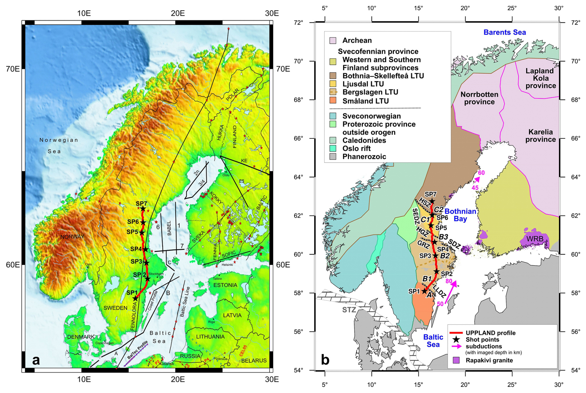
Figure 1 Location of the UPPLAND profile and previous refraction seismic profiles within the study area (a). Seismic profile superimposed on a tectonic sketch map (modified after Buntin et al., 2021) (b). Tectonic units: A – Småland Terrane; B1 – Sörmland Basin; B2 – Uppland Batholith; B3 – major deformation zone; C1 – Ljusdal Batholith; C2 – Bothnian Basin. Magenta lines: dip of Proterozoic subductions imaged seismically. Lithotectonic units (LTUs) after Stephens and Bergman (2020). GRZ – Gävle–Rättvik Zone; HGZ – Hagsta Gneiss Zone; HSZ – Hassela Shear Zone; LLDZ – Linköping–Loftahammar Deformation Zone; SDZ – Singö deformation zone; WRB – Wiborg rapakivi batholith; SEDZ – Storsjön–Edsbyn Deformation Zone; STZ Sorgenfrei–Tornquist Zone. Stars represent shot points, and dots represent receivers.

After the publication of these results, our alternative model can now be presented. The paper presents the re-analysis of seismic data and calculated tests of the competitive models for the V_p and V_s velocities and the $V_{\mathrm{p}}/V_{\mathrm{s}}$ ratio for the UPPLAND profile. From several seismic models of P- and S-wave velocities and $V_{\mathrm{p}}/V_{\mathrm{s}}$ ratio which fit the travel time data, we selected one and present it in Fig. 4 as our best solution. We also discuss tectonic interpretations combining existing geological information with the new model.

2 Fieldwork and seismic data

The UPPLAND profile is ∼ 540 km long (Fig. 1a). There were seven shot points (SPs) located at distances from ∼ 60 to ∼ 135 km and with charges of 360–500 kg of explosive. Seismic energy was recorded by 595 short-period receivers. For more details, see Buntin et al. (2021) and Figs. A1 and A2.

2.1 P wave

The first arrivals of P_g waves are clearly visible at offsets up to approximately ∼ 187–220 km in all recorded seismic sections and in the section for SP7, even up to approximately 260 km (Figs. 2 and 3). Apparent velocities (V_app) vary from ∼ 6 to ∼ 6.75 km s⁻¹.

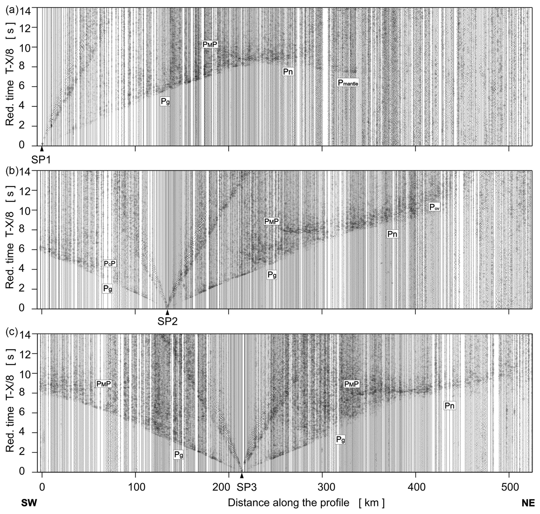
Figure 2 Examples of trace-normalised, vertical-component seismic record sections for P wave, SP1–SP3. Band-pass filters, 2–15 Hz, have been applied. P_g: P refractions from the upper and middle crystalline crust; P_ov: P overcritical crustal phases; P_cP: P reflections from the mid-crustal discontinuities; P_MP: P reflections from the Moho boundary; P_n: P refractions from the sub-Moho upper mantle; P_mantle: lower-lithospheric P phases. The reduction velocity is 8.0 km s⁻¹.

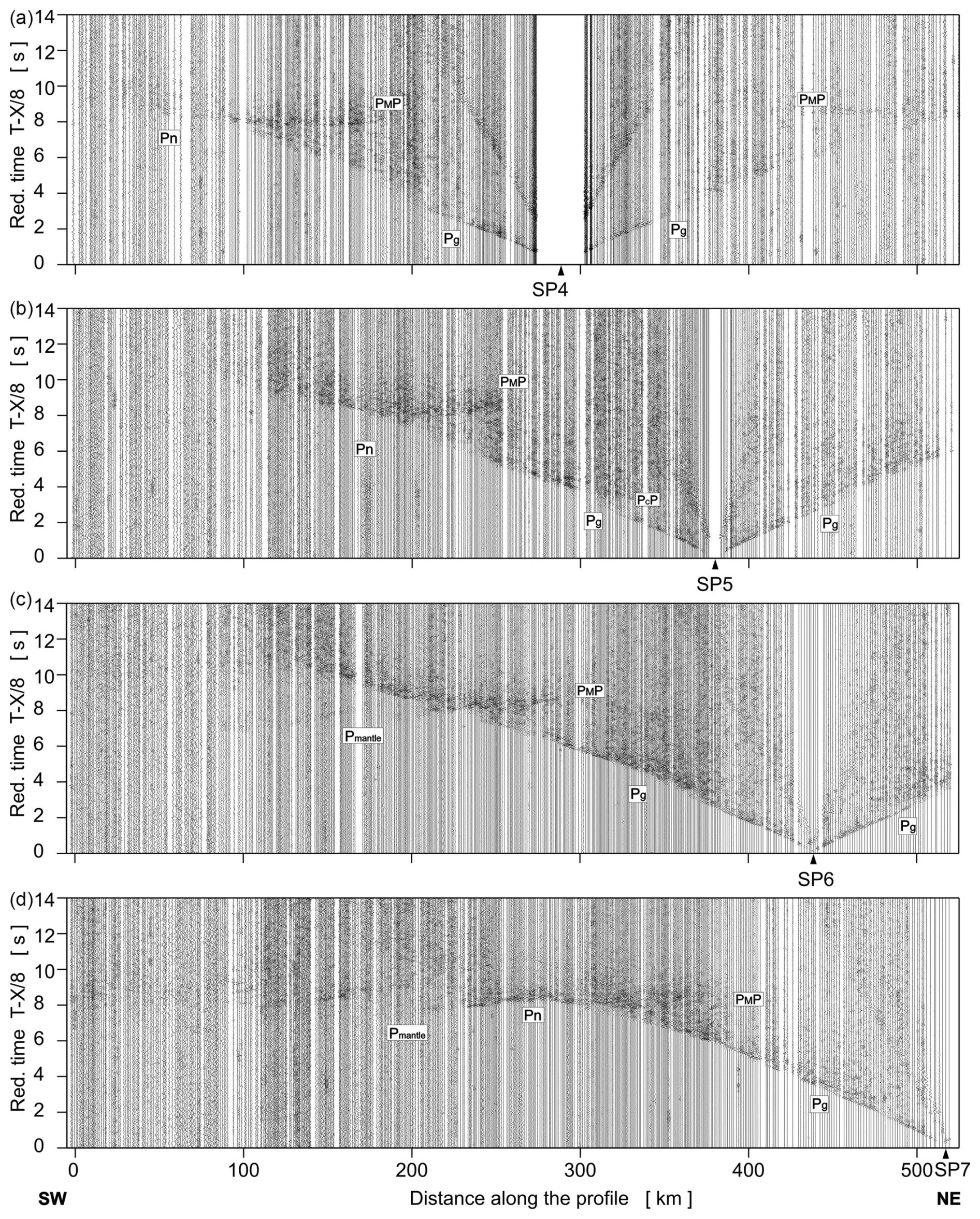
Figure 3 Examples of trace-normalised, vertical-component seismic record sections for P wave, SP4–SP7. Other abbreviations are as in Fig. 2.

In several sections for further offsets, the apparent velocities of the first arrivals V_app>7 km s⁻¹ are observed: SP1 from ∼ 219 to ∼ 235 km, V_app∼7.2 km s⁻¹; SP2 (right) from ∼ 192 to ∼ 267 km, V_app∼7.0–7.1 km s⁻¹; SP4 (right) from ∼ 188 to ∼ 237 km, V_app∼7.3 km s⁻¹; SP5 (left) from ∼ 191 to ∼ 209 km, V_app∼7.1 km s⁻¹. However, due to the relatively high noise, it is not certain whether they really represent first arrivals or if they perhaps represent later arrivals, and the actual first arrivals disappear in the noise.

In several sections (but not in all of them) at large offsets, clear arrivals are visible, which, judging by the apparent velocities, arrive from the upper mantle (UM): SP1 P_n (∼ 235–262 km, V_app∼8 km s⁻¹) and P_mantle (∼ 262–350 km, V_app∼8.75 km s⁻¹); SP3 (right) P_n (∼ 216–253 km, V_app∼7.75 km s⁻¹); SP6 (left) P_mantle (∼ 216–253 km, V_app∼8.75 km s⁻¹); SP7 (left) P_n (∼ 231–254 km, V_app∼8 km s⁻¹) and P_mantle (∼ 254–300 km, V_app∼8.75 km s⁻¹).

2.2 S wave

The S-wave sections also are of good quality (Figs. A1 and A2). However, the first appearances of S_g waves are not clearly visible at offsets up to approximately ∼ 156–257 km, depending on the size of the charges used to excite the energy. Apparent velocities vary from ∼ 3.5 to ∼ 3.75 km s⁻¹.

For the two sections with the highest charges, clear pulses with high apparent velocities are visible, probably coming from the upper mantle: SP1 S_n (∼ 241–261 km, V_app∼4.5 km s⁻¹) and S_mantle (∼ 261–368 km, V_app∼5 km s⁻¹); SP7 S_mantle (∼ 257–283 km, V_app∼5 km s⁻¹).

3 Seismic modelling

3.1 Trial-and-error iterative forward modelling

The modelling of travel times, rays, and synthetic seismograms was performed using the SEIS83 package (Červený and Pšenčík, 1984) with support from the programs MODEL (Komminaho, 1998) and ZPLOT (Zelt, 1994) with modifications by Środa. Our calculated V_p model (Fig. 4) for the upper and middle crust seems quite unambiguous, although, at first glance, it clearly seems different from the model of Buntin et al. (2021) and Fig. A3. Both models, despite quite significant differences in terms of the geometry of the boundaries, present similar velocities V_p and V_s (±0.1 km s⁻¹) down to a depth of ∼ 35 km. The main differences concern the velocities in the lower crust (LC) and the upper mantle and the depth of the Moho boundary. Determining the velocity in the lower crust from seismic sections is often problematic, as the lower-crustal refractions typically show in the seismic section as later arrivals and may easily be obscured by the first arrivals' coda.

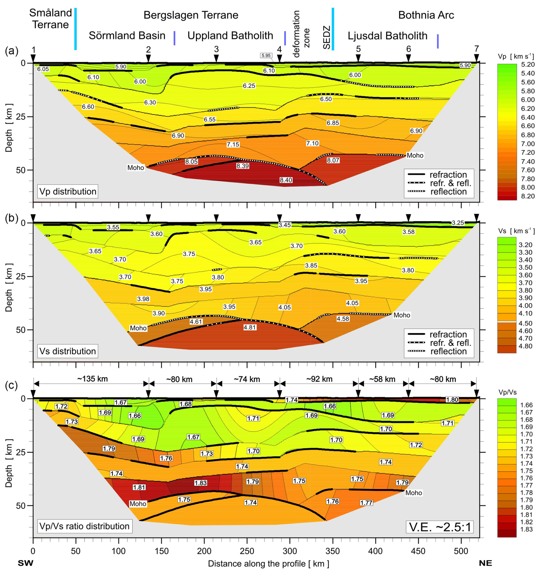
Figure 4 2D models of seismic P- and S-wave velocity in the crust and upper mantle derived by forward ray-tracing modelling using the SEIS83 package (Červený and Pšenčík, 1984) along the UPPLAND profile. (a) P-wave velocity model. Thick black lines represent major velocity discontinuities (interfaces). (b) S-wave velocity model. (c) Model of $V_{\mathrm{p}}/V_{\mathrm{s}}$ ratio distribution. Thick black solid and dashed lines represent major velocity discontinuities (boundaries). Only those parts of the discontinuities that have been constrained by reflected or refracted arrivals of P or S waves are shown: solid line – refraction only; dashed line – refraction and reflection; dotted line – reflection only. Thinner lines represent inferred velocity isolines with values (in km s⁻¹) shown in white boxes. The positions of tectonic units at the surface are indicated. Inverted triangles show the positions of shot points. Vertical exaggeration is ∼ 2.5:1 for the model.

Using the SEIS83 code, several solutions were tested with different velocities for the lower crust and upper mantle. We conducted tests using three models with different velocities in the lower crust (LC) and upper mantle (UM), Figs. A9–A11. Model 1 contained two layers (V_p=7.1–7.15 km s⁻¹ and V_p∼7.25–7.4 km s⁻¹ for LC and V_p∼8.4 km s⁻¹ for UM), closely resembling values from the model of Buntin et al. (2021). Models 2 and 3 had only one layer, V_p∼7.05–7.17 km s⁻¹, for LC and two layers with V_p∼8.05 and V_p∼8.4 km s⁻¹ for UM. Models 2 and 3 differ in their UM velocities, particularly in the central part of the profile. Comparing the theoretical and experimental travel times in the seismic sections for P- and S-wave models enabled us to conclude that all three models fall within the class of models acceptable for the specified task, i.e. satisfying available travel time data. However, Model 3, with the best fit (see tests in Appendix A), is our preferred choice. In this model, the depth of the Moho boundary varies in the range of ∼ 44 km (S), ∼ 50 km (central part), and ∼ 42 km (N). The $V_{\mathrm{p}}/V_{\mathrm{s}}$ values in the LC vary from 1.81 to 1.83 and 1.75 to 1.79 along the profile from S to N, and, for the UM, they range from 1.74 to 1.77. Modelling examples for our Model 3, for both P and S waves, are presented in Figs. 5 and 6 and Figs. A4–A8. In the Appendix, we present all three tested models (Figs. A9–A11) for V_p, V_s, and $V_{\mathrm{p}}/V_{\mathrm{s}}$ distribution, but their calculated residuals are presented in Tables A1 to A6.

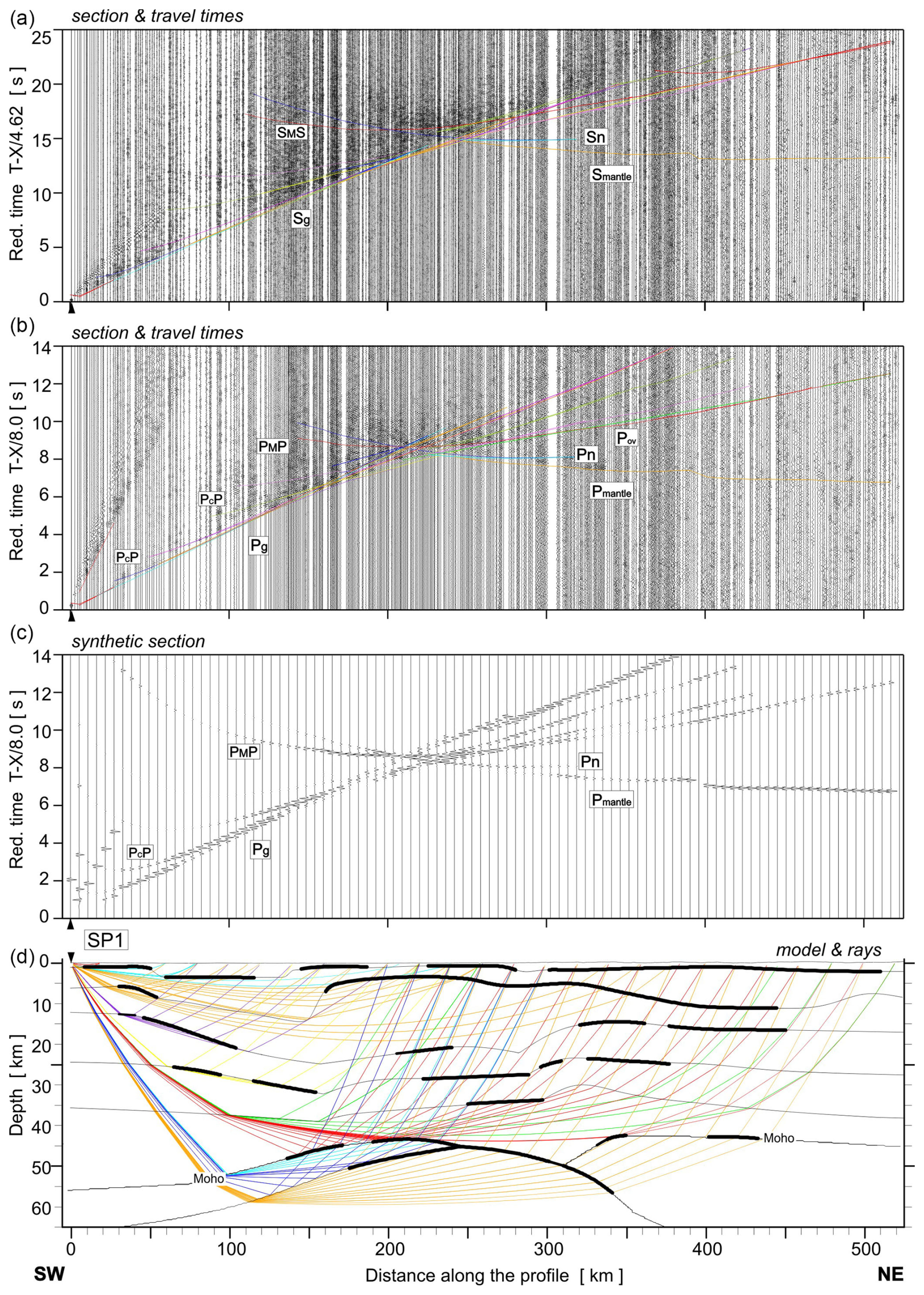
Figure 5 Examples of seismic modelling along the UPPLAND profile for SP1; seismic record sections (amplitude-normalised vertical component) of S and P wave with theoretical travel times calculated using the SEIS83 ray-tracing technique. (a) For S wave, we used the band-pass filter of 1–12 Hz and the reduction velocity of 4.62 km s⁻¹. (b) P-wave data have been filtered using the band-pass filter of 2–15 Hz and displayed using the reduction velocity of 8.0 km s⁻¹ for P wave. (c) Synthetic seismograms and (d) ray diagram of selected rays of P wave. All examples were calculated for the models presented in Fig. 4. Other abbreviations are as in Fig. 2.

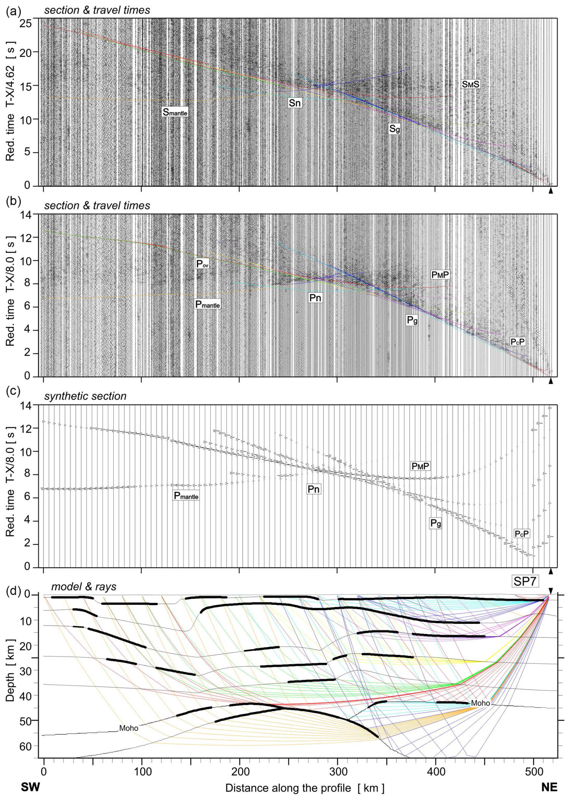
Figure 6 Examples of seismic modelling along the UPPLAND profile, for SP7. Other abbreviations are as in Fig. 5.

3.2 Uncertainty of the trial-and-error model

The fit of the individual phases of P and S waves in Model 3 is shown in Figs. 7 and 8. At the top (part a), we present the differences between theoretical (black points) and observed (coloured points) travel times. In the middle (part b), we present travel time residuals, and, at the bottom (part c), the ray coverage from forward modelling along the profile is shown. We distinguish the P_g arrivals (green points), P_cP arrivals (blue points; reflections in the crust without P_MP phase), P_MP arrivals (red points), and P_n arrivals (brown points). The P_g phase has a good fit along the whole profile in Model 3. The largest residuals are observed for the P_MP phase in the central part of the profile.

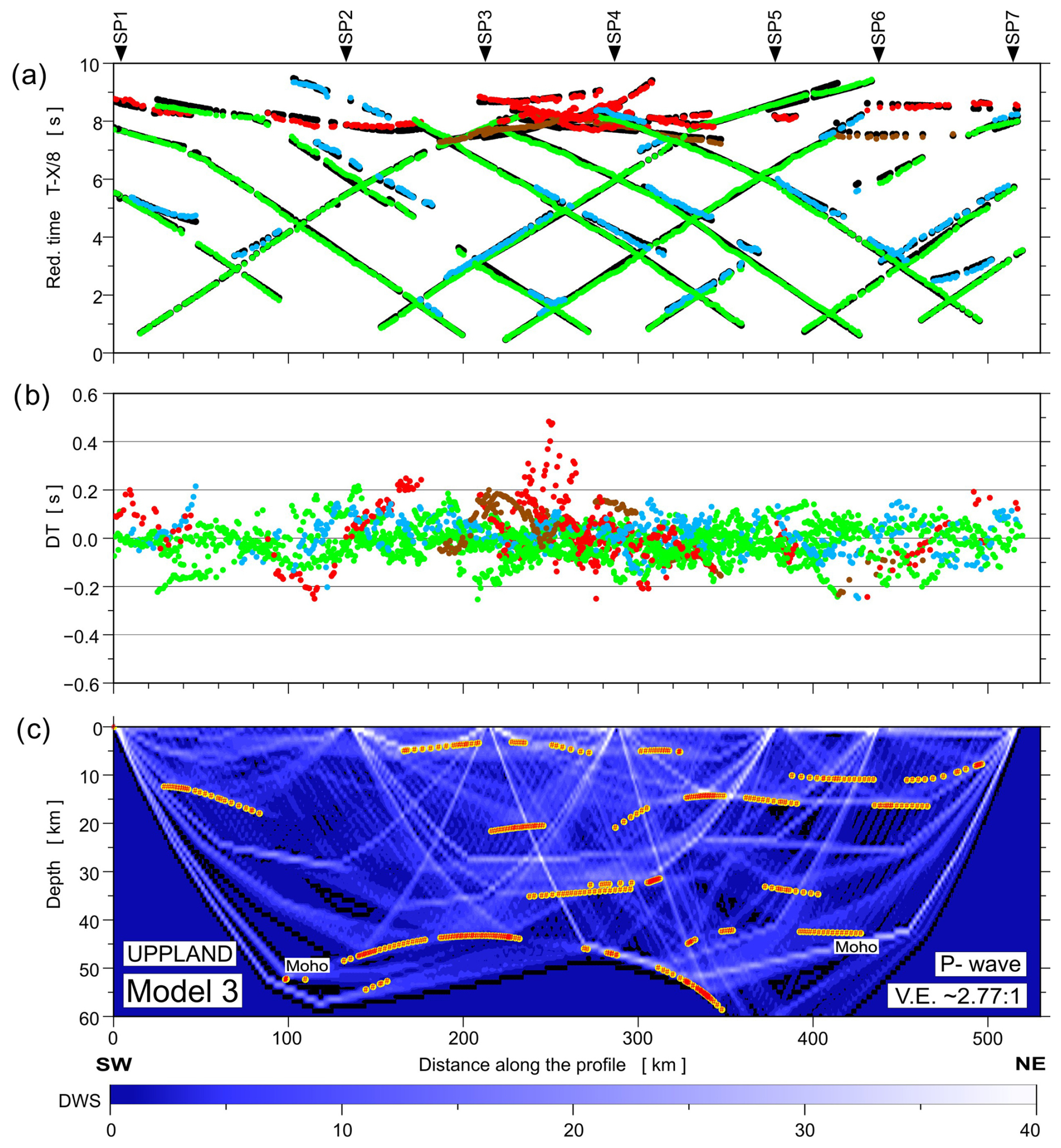
Figure 7 Diagrams showing theoretical and observed travel times (a), travel time residuals (b), and schematic ray coverage (c) from forward modelling along the profile. Green points – P_g arrivals; blue points – P_cP arrivals (reflections in the crust without P_MP); red points – P_MP arrivals; brown points – P_n arrivals; black points – theoretical travel times; yellow lines – schematic fragments of discontinuities constrained by reflected phases for P-wave velocity Model 3. The red points plotted along the interfaces mark the theoretical bottoming points of reflected phases (every third point is plotted), and their density is a measure of the positioning accuracy of the reflectors. DWS – derivative weight sum. The reduction velocity is 8.0 km s⁻¹.

Figure 8 Diagrams showing theoretical and observed travel times (a), travel time residuals (b), and schematic ray coverage (c) from forward modelling along the profile. Green points – S_g arrivals; blue points – S_cS arrivals (reflections in the crust without S_MS); red points – S_MS arrivals; brown points – S_n arrivals; black points – theoretical travel times; yellow lines – schematic fragments of discontinuities constrained by reflected phases for S-wave velocity Model 3. Other abbreviations are as in Fig. 7. The reduction velocity is 4.62 km s⁻¹.

A similar analysis was made for models 1 and 2, as shown in Figs. A12–A15. Here, we have also shown differences between theoretical and observed travel times, travel time residuals, and schematic ray coverage from forward modelling along the profile for each model separately. The P_g phase shows a good fit for all shot points. For other phases, in particular for the P_MP phase, the largest residuals are in the middle part of the profile.

For each model, the RMS values were calculated separately for all P-wave and S-wave phases (in Model 1, the P_n1 phase does not occur). The calculated RMS values for each P and S phase for all analysed models are shown in Tables A1 to A6. The P-wave RMS residuals range from 0.07 (P_g phase) to 0.23 s (P_MP phase) for Model 1, from 0.07 (P_g) to 0.19 s (P_MP) for Model 2, and from 0.07 (P_g) to 0.13 s (P_MP) for Model 3. For S wave, respective residuals are much larger – from 0.28 to 0.39 s for Model 1 and from 0.14 to 0.26 s for Model 2. Model 3 gives the lowest S-wave residuals – 0.14 s for S_g phase and 0.18 s for S_MS phase. Large residuals for S waves are mainly due to high picking uncertainties of S phases.

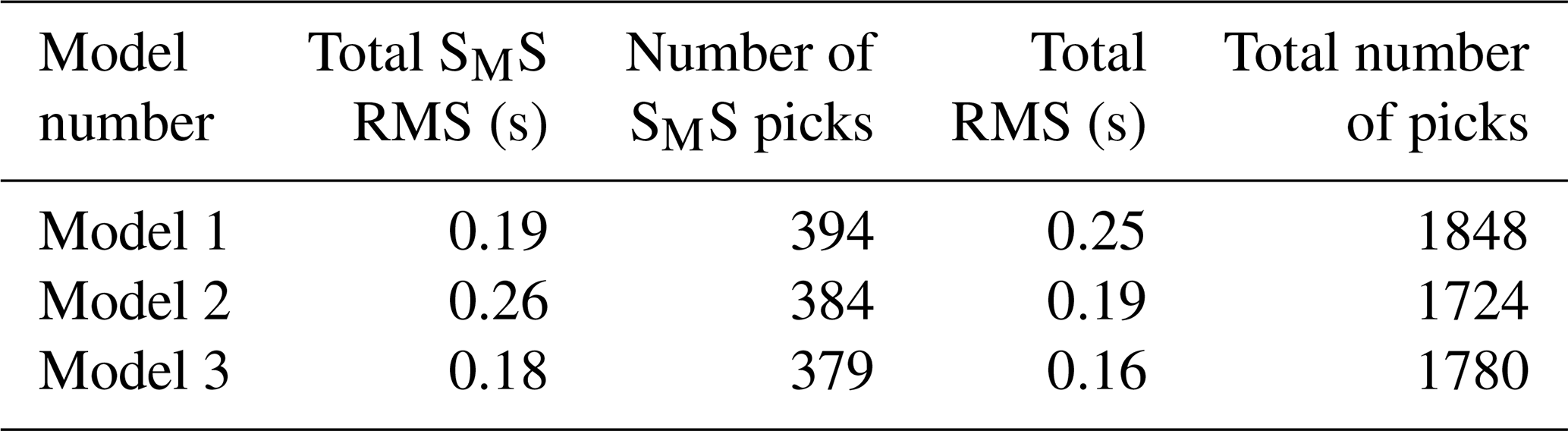
The total RMS residuals for P and S phases for all models are presented in Tables 1 and 2, respectively. Although for different P waves the differences between the models are not significant, for S waves, they are substantial. It can be noted that Model 3 has the best fit to the data, both for P waves and S waves. Additionally, the RMS values for the P_MP and S_MS phases are summarised in Tables 1 and 2, respectively. As before, the RMS differences for the S_MS waves are more significant than for the P_MP waves, and Model 3 shows the best fit to the data.

Table 1 RMS residuals calculated for the analysed models for both P_MP-phase and total values with the respective number of picks.

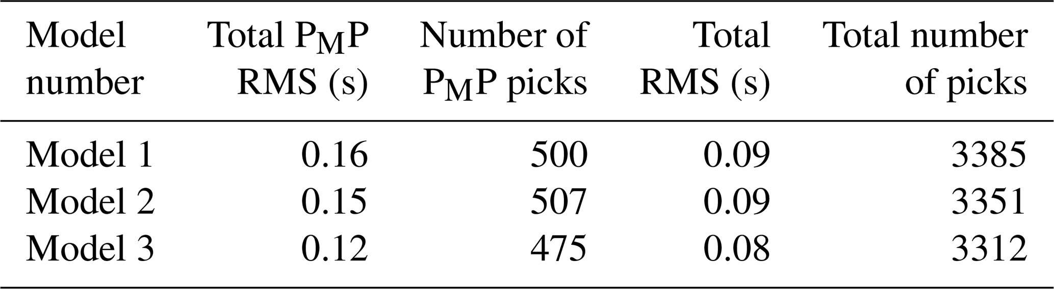
Table 2 RMS residuals calculated for the analysed models for both S_MS-phase and total values with the respective number of picks.

3.3 Refraction travel time tomography

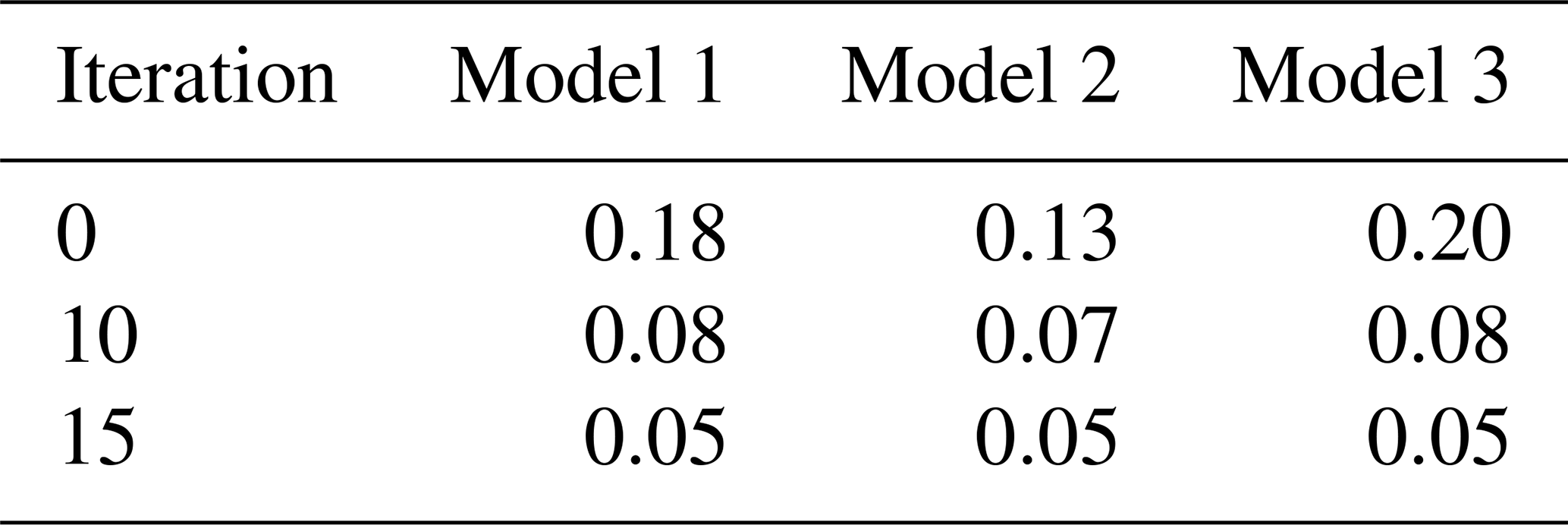
In order to check which velocity model will be obtained using first arrivals (P_g + P_n) only and to get an estimate of the non-uniqueness of such model, a tomographic inversion of the P-wave first arrivals of the UPPLAND profile was conducted using the back-projection method proposed by Hole (1992) with various initial models. A 2D model size of 540×70 km was chosen. For preparation of the initial models for the 2D inversion, firstly, a 1D average-velocity model was calculated using the Wiechert–Herglotz inversion method. The input for the Wiechert–Herglotz method was an average travel time curve obtained from all first-arrival picks. Then, the mantle velocity was changed to produce three variants of the initial models with mantle V_p of 7.4–7.5 km s⁻¹ (Model A), 8.0–8.2 km s⁻¹ (Model B), and 8.2–8.4 km s⁻¹ (Model C). The first inversion steps were carried out for picks up to 60 km offset, and, in subsequent iterations, offsets were increased up to 540 km in five steps in order to gradually increase the penetration depth of the seismic rays. In total, 2270 travel times were used in the inversion process. In each iteration, smoothing filters were applied to the velocity corrections. The size of the filter was decreased with iteration number (three sizes of the smoothing filters were used) in order to gradually increase the resolution. The velocity grid spacing was 1×1 km. For the calculation of the final model, 45 iterations in total were used. The initial models produced RMS residual of 0.17–0.3 s, while the final RMS travel time residual reached for all models was 0.05 s. When considering the estimated picking accuracy to be ∼ 0.1 s, the initial RMS residual for some of the models was low, showing that even the initial models show a relatively good fit to the data. This is most likely due to a lateral homogeneity of most of the crust along the profile. The lateral differentiation of the V_p apparently occurs only at lower-crustal/upper-mantle depths, affecting only a small part of travel times (corresponding to deep P_g rays and P_n rays) and resulting in relatively good overall travel time fit even for 1D initial models. The final models are presented in Fig. A16. It can be seen that, in all three models, the main modification of the V_p velocity field resulting from inversion is the increase of the mantle velocities at a depth of ∼ 45–60 km in the central part of the model, in ∼ 120–340 km distance range, similarly to SEIS83 forward models.

Other variants of the inversion were done with initial models derived from 2D SEIS83 ray-tracing models 1, 2, and 3. This was done in order to verify the travel time fit of these models to first arrivals data and to check which parts of the models will be modified by the inversion. The result is presented in Fig. A17. The RMS residual for these initial models was 0.13–0.20 s (Table A7), close to the estimated picking uncertainty, confirming a good travel time fit for those 2D ray-tracing models. Nevertheless, in the final inversion models, we can observe modifications of the V_p distribution, located mainly in the upper mantle of the central part of the model (200–300 km distance) and in the lower crust in its NE part (320–400 km distance). In the effect of the inversion, the high mantle V_p decreased at ∼ 200 km distance and increased at ∼ 300 km distance, shifting the updomed area of high mantle velocities some 70 km to the NE. Also, the lower-crustal velocities at ∼ 340–400 km distances were increased by the inversion. However, these changes with respect to the SEIS83 models may result from using first arrivals only, and SEIS83 models using all refracted and reflected phases should be considered more reliable. Final RMS residuals after inversion were 0.05 s.

4 Discussion

4.1 Limitations in wide-angle seismic modelling of the lower crust

We try to describe the problems we encounter when constraining the properties of the lower crust (thickness, seismic wave velocity, heterogeneity) and to discuss the potential limitations of the method. Generally, using wide-angle reflection and refraction, the possible sources of information on the lower-crust properties are

• the first arrivals of the P wave refracted in the lower crust;

• the Moho reflections at overcritical distances;

• the ringing character of the P-wave signal reflected from or penetrating the lower crust, which gives hints about the fine structure (e.g. lamination) of this layer;

• S-wave arrivals (if observed) allowing determination of the $V_{\mathrm{p}}/V_{\mathrm{s}}$ ratio distribution.

Depending on the actual crustal structure and the resulting observed wide-angle wavefield, information about the lower crust can be ambiguous or substantially limited. Non-uniqueness of some parts of the wide-angle model is an inherent feature of this method.

The most appropriate information to determine the velocity of the top of the lower crust (LC) is the first arrivals of seismic waves refracted from this boundary. In many cases, the accuracy of the LC modelling can be improved by well-recorded overcritical P_MP waves that penetrate the lower crust. However, waves refracted from the lower crust are rarely observed in the first arrivals. In order for them to show up in the first pulses, a sufficiently large LC thickness is needed, e.g. as it is in the Central Finland Granitoid Complex. Apparent velocities higher than 7 km s⁻¹ are seen in most of the record sections at offsets from 185 up to 290 km of the FENNIA and SVEKA'81 profiles (Janik et al., 2007).

When planning a new wide-angle reflection and refraction profile, the number of shot points must be determined. This depends on the length of the planned profile and the degree of complexity of the crust structure and its expected depth. Considering the high costs of drilling and shooting works, the financial resources available are a major limitation in planning. The optimal distances between adjacent shot points (SPs) should be within the range of $\mathrm{1}/\mathrm{2}$ H–H (where H is the expected crust thickness). Of course, the denser the network of shot points and the better the quality of the recorded sections, the better the final model can represent the complex structure. The distances between SPs on the UPPLAND profile are usually much larger than is optimal, as their average is ∼ 90 km. An additional problem is the deviation of the shot points from the straight line of the profile, e.g. for SP1 (∼ 80 km) and, to a lesser extent, for SP5 (∼ 15 km). With such a profile geometry, it is difficult to achieve high model accuracy.

Data from the UPPLAND profile do not enable us to clearly determine the structure of the lower crust. In cases where there is high ambiguity in the measured data, it seems prudent to explore other solutions, particularly for the lower crust. This ambiguity not only strongly impacts the determination of the Moho boundary's depth but also influences the petrological and tectonic interpretation of the studied area. These problems also affect the interpretations discussed below.

The European Moho depth map (Grad et al., 2009) indicates that UPPLAND profile is located on a Moho slope dipping towards the east. The depth of the Moho boundary presented on the BABEL 6 line (Buntin et al., 2019), 50–60 km, is about 5–10 km greater than on the corresponding fragment of our UPPLAND profile model. One of the reasons may be the use of different mean velocities in the crust during processing. The second reason may be the actual change of depth, which, judging from the European Moho depth map (Grad et al., 2009), tends to increase eastward (by ∼ 3–4 km) from the northern part of the UPPLAND profile to BABEL 6. In any case, we used the information about the Moho surface geometry in our initial interpretation.

4.2 Implications for tectonic evolution

The UPPLAND seismic profile (Figs. 1 and 9) crosscuts 1.9–1.8 Ga cratonic crust in southern central Sweden, Fennoscandia. The profile starts from the Småland lithotectonic unit characterised by 1.83–1.82 Ga volcanic arc (OJB) surrounded by 1.81–1.77 Ga granitoids and volcanic rocks (Wahlgren and Stephens, 2020). The Bergslagen lithotectonic unit (Stephens and Jansson, 2020) includes 1.91–1.88 Ga volcanic arc rocks and, in the northern and southern parts, 1.87–1.84 Ga granitoids. The Ljusdal lithotectonic unit is dominated by 1.87–1.84 Ga granitoids (Högdahl and Bergman, 2020), and the profile ends in the Bothnia–Skellefteå lithotectonic unit, including 1.87–1.84 and 1.81–1.77 Ga granitoids (Skyttä et al., 2020). West of these units occurs a large 1.7 Ga magmatic province, which is in part strongly reworked during the Sveconorwegian orogeny (Ripa and Stephens, 2020a). In northern Bergslagen (close to shot point 4; Fig. 9) occurs an E–W-trending basin of younger 1.6–1.4 Ga magmatism and Mesoproterozoic sedimentary rocks (Bergman et al., 2012). Rapakivi granites, both observed and interpreted (Korja and Heikkinen, 2005; Ripa and Stephens, 2020b), are found east of the UPPLAND profile (Fig. 9a). Younger minor magmatic stages (not shown) are seen as dykes and other hypabyssal rocks at 1.27–1.25 Ga in the northern part of the profile and as NNW–SSE-trending ca. 1.0 Ga dolerites in western and central Bergslagen (Bergman et al., 2012).

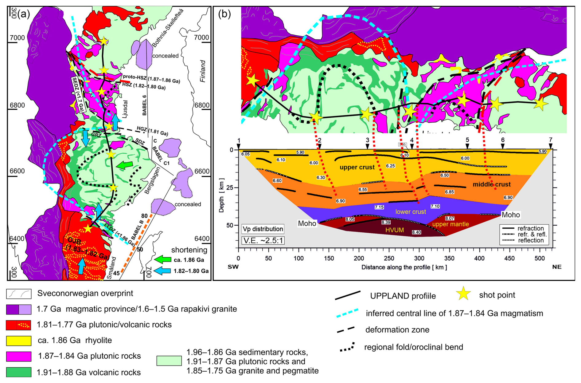
Figure 9 (a) Simplified geological map of the UPPLAND profile and its surroundings based on descriptions by Högdahl and Bergman (2020), Ripa and Stephens (2020a, b), Skyttä et al. (2020), Stephens and Jansson (2020), Wahlgren and Stephens (2020), and Korja and Heikkinen (2005). Rocks younger than 1.6 Ga are not shown here, but ≥1.70 Ga rocks reworked in younger orogens are included. The regional folds are from Stephens (2020) (see Beunk and Kuipers, 2012), and the ca. 1.86 Ga shortening direction is from Stålhös (1981). BABEL profiles (thin lines) and Moho to upper-mantle reflectors (dashed orange line with imaged depth in km) are from Abramovitz et al. (1997). GRZ = Gävle–Rättvik Zone; HGZ = Hagsta Gneiss Zone; HSZ = Hassela Shear Zone; LLDZ = Linköping–Loftahammar Deformation Zone; SDZ = Singö deformation zone; SEDZ = Storsjön–Edsbyn Deformation Zone; OJB = Oskarshamn–Jönköping Belt. (b) Rotated section from the geological map (upper) and modified seismic model along the profile (lower). Dotted red lines show selected geological structures tentatively projected into the seismic model. HVUM = high-velocity upper mantle.

The lithotectonic units are bounded by deformation zones (Fig. 9a), which are zones of gneiss and ductile shear, often kilometres wide, overprinted by localised deformation zones at 1.82–1.80 Ga (for details, see references in Fig. 9). The dextral strike-slip component is dominant, and, locally, ca. 1.86 Ga older shear deformation is observed. The Storsjön–Edsbyn Deformation Zone (SEDZ) is younger and probably related to the 1.7 Ga magmatic province. The main stages of deformation and metamorphism in the Småland, Bergslagen, and Ljusdal lithotectonic units (for references, see above) occurred at ca. 1.86 Ga (1.87–1.85 Ga) and at 1.82–1.80 Ga (1.84–1.80 Ga). The large regional fold in Bergslagen (Fig. 9a; Stephens, 2020) correlates with the Bergslagen orocline of Beunk and Kuipers (2012). Lahtinen et al. (2023) proposed that Ljusdal and the Mid-Baltic belt of Bogdanova et al. (2015), including the southernmost part of the Bergslagen lithotectonic unit, are parts of a single, originally linear belt characterised by 1.87–1.84 Ga arc magmatism (Fig. 9a).

The tectonic evolution at 1.9–1.8 Ga in the study area has been considered to represent an accretionary orogen in which the crust is stacked sequentially, leading to the lateral growth of the orogen towards the southwest (Gorbatschev and Gaál, 1987; Korja and Heikkinen, 2005; Bogdanova et al., 2015; and references therein). Based on the more generic tectonic switching model by Collins (2002), an episodic evolution containing several extension–contraction cycles in SW-retreating, active continental margin at 1.90–1.80 Ga has been proposed (e.g. Hermansson et al., 2008; Stephens, 2020). Thus, either a single subduction system with intervening crustal shortenings due to flat subduction (e.g. Hermansson et al., 2008) or several subduction–collision pairs (e.g. Korja and Heikkinen, 2005; Buntin et al., 2021) are proposed. The occurrence of arc rocks of similar age (1.91–1.89 Ga) in Fennoscandia has been suggested to represent a ≥2000 km long arc system affected by an orocline-forming event (Lahtinen et al., 2014), which may have included the separation of Bergslagen from the linear arc (Lahtinen et al., 2023). The current structural trends in Bergslagen resulted from the late-orogenic major folding (oroclinal bending) of originally NW–SE-oriented structures (Beunk and Kuipers, 2012; Stephens, 2020).

We use the preferred seismic model of this study in our interpretation (Fig. 9b). The proposed palaeosubduction zone (Figs. 1 and 9a) could be related to 1.86 and/or 1.82–1.80 Ga flat subduction stages. The N-dipping structures in the upper and middle crust of the seismic model (Fig. 9b) are correlated with N–S crustal shortening (Fig. 9a). The thick upper crust and bulging of the upper mantle (HVUM in Fig. 9b) under Bergslagen occur below the proposed regional fold and the oroclinal bend of 1.87–1.84 Ga magmatism (Fig. 9b). The latter structure ends to a wide deformation zone composed of the GRZ and HGZ (Fig. 9a and b). The depth of the Moho boundary increases abruptly at the end of the BABEL B profile and continues as such in BABEL C1 (Korja and Heikkinen, 2005), correlating with the UPPLAND model (Fig. 9a and b). The Bergslagen–Ljusdal boundary zone is characterised by an upward-expanding and thickening lower crust and a bulging of the upper mantle (Fig. 9b). Similar thickening of the lower crust in BABEL C is interpreted as due to N-vergent crustal stacking of the lower crust (Korja and Heikkinen, 2005). We propose a viable tectonic model where the mantle bulge and thinning of the lower crust are related to the ca. 1.89–1.87 Ga extension in a back-arc setting of an NW–SE-trending continental arc. Subsequent WSW-directed basin inversion at ca. 1.86 Ga was followed by nearly orthogonal shortening at 1.82–1.80 Ga, leading to oroclinal bending and crustal stacking.

The bulging of the high-velocity upper mantle and two upper-mantle layers and the lack of high-velocity lower crust in the seismic model (Figs. 4 and 9b) are comparable with the seismic structure under the Wiborg rapakivi batholith (Fig. 1b; Janik, 2010; Tiira et al., 2022). The possibility exists that the abovementioned mantle–lowermost crust structure in the UPPLAND profile formed during the 1.8 and/or 1.7 Ga magmatic stage(s) or during the 1.6–1.5 Ga stage (Fig. 9a). IN particular, the 1.7 Ga magmatic province seems to have been a very large province, originally extending to the west and possibly also to the east under Bergslagen and Ljusdal (Fig. 9a). The occurrence of rapakivi granites and related rocks in the N–S array (Fig. 9a) could also fit to large-scale extension, mantle bulging, and melting of lower crust. Based on the European Moho depth map (Grad et al., 2009), the UPPLAND profile is located on a Moho slope dipping towards the east; thus, the bulging of the high-velocity upper mantle, if ≤1.8 Ga in age, is more likely related to processes in the west than in the east.

The main problem in the interpretation of the upper- to middle-crustal structures along the UPPLAND profile is that the ca. 1.86 Ga crustal stacking, preceding the 1.82–1.80 Ga folding and stacking, had vergence towards W, nearly orthogonal to the profile (Fig. 9a). Needed 3D information would require an E–W-oriented seismic profile across Bergslagen. As discussed in this paper, the information about the lower crust and Moho boundary can be ambiguous. Also, the age (1.9, 1.8, 1.7, or 1.6–1.5 Ga or younger) of the lower-crust and upper-mantle structures is unknown. Based on existing geological information and tectonic models, two possible interpretations of the studied area are discussed above. These models could even be a diachronic process where the high-velocity upper mantle–lowermost crust stabilised at 1.7 Ga or 1.6–1.5 Ga and thus >100–300 Ma later than the formation of main parts of the crustal structure at 1.82–1.80 Ga.

A contradictory model of solely northward subduction, including a collision between Bergslagen and Ljusdal, was proposed by Buntin et al. (2021). They interpreted the high-velocity body (HVUM in Fig. 9b) as a mafic lowermost-crustal layer partially transformed into a ca. 150–200 km long and 6–8 km thick eclogite body during Palaeoproterozoic orogeny. Interestingly, the high-velocity upper mantle (V_p∼8.30–8.37 km s⁻¹) under the Wiborg rapakivi batholith is at least 250 km long (Tiira et al., 2022) but is apparently related to the formation of the rapakivi batholith, occurring >150 Ma later than stabilisation of the orogenic crust.

5 Conclusions

Our re-analysis of seismic data and the calculated competitive models for the V_p and V_s velocities and the $V_{\mathrm{p}}/V_{\mathrm{s}}$ ratio for the UPPLAND profile show similar velocities V_p and V_s (±0.1 km s⁻¹) up to a depth of ∼ 35 km as in the model by Buntin et al. (2021). The main differences between these two models include significant differences in terms of the geometry of the boundaries, the velocities in the lower crust and upper mantle, and the depth of the Moho boundary.

Two, possibly overlapping, tectonic interpretations are proposed to explain the new model. The main crustal structure formed during W-vergent crustal stacking at ca. 1.86 Ga followed by N–S shortening at 1.82–1.80 Ga. The bulging of the high-velocity upper mantle is related to extension at 1.89–1.87 Ga in a continental back-arc or to extensional magmatism at 1.6–1.5, 1.7, and/or 1.8 Ga.

Appendix A

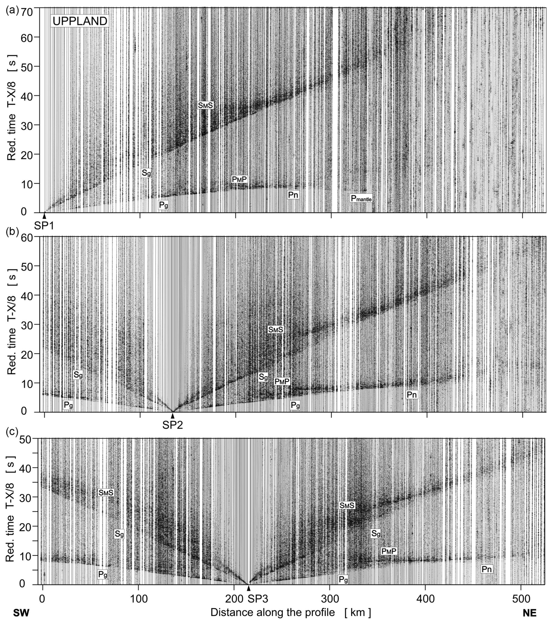
Figure A1 Examples of trace-normalised, vertical-component seismic record sections for P and S wave, SP1–SP3. A band-pass filter of 2–15 Hz has been applied. P_g: P refractions from the upper and middle crystalline crust; P_ov: P overcritical crustal phases; P_cP: P reflections from the mid-crustal discontinuities; P_MP: P reflections from the Moho boundary; P_n: P refractions from the sub-Moho upper mantle; P_mantle: lower-lithospheric P phases. Respective abbreviations have been used for S wave. The reduction velocity is 8.0 km s⁻¹.

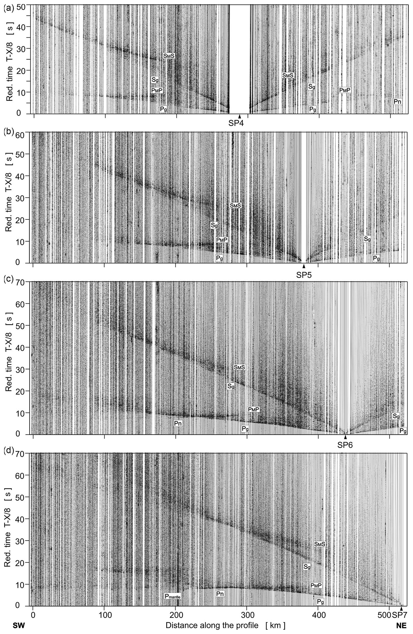
Figure A2 Examples of trace-normalised, vertical-component seismic record sections for P and S wave, SP4–SP7. Other abbreviations are as in Fig. A1.

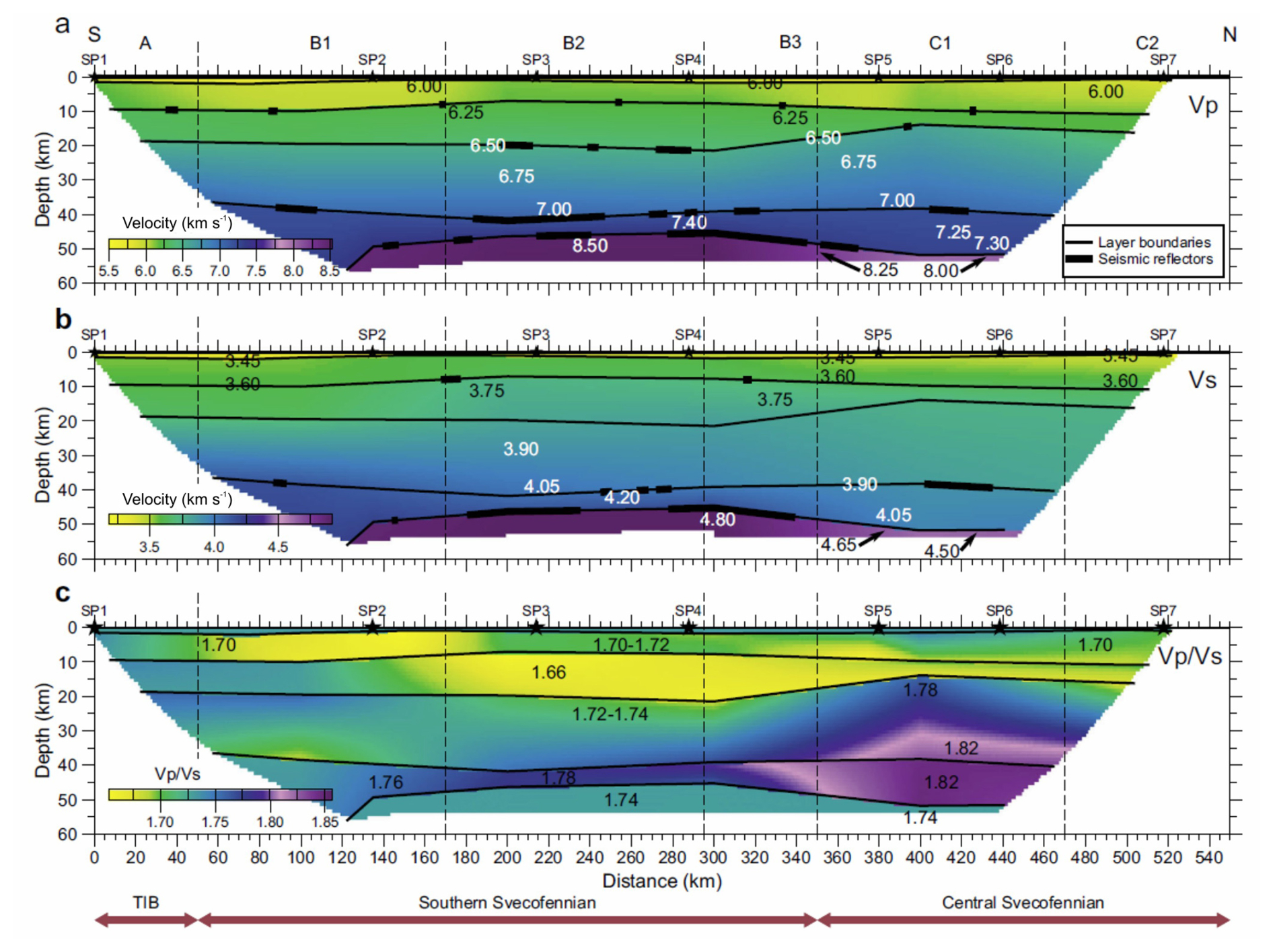
Figure A3 Seismic models along the profile. (a) P- and (b) S-wave velocity and (c) $V_{\mathrm{p}}/V_{\mathrm{s}}$ ratio along the seismic profile (modified after Buntin et al., 2021). Seismic sources (SP1–SP7): black stars; tectonic units as in Fig. 1 (main part). Velocity discontinuities – dashed lines; identified seismic reflections – thick black lines (shown in panels a and b only).

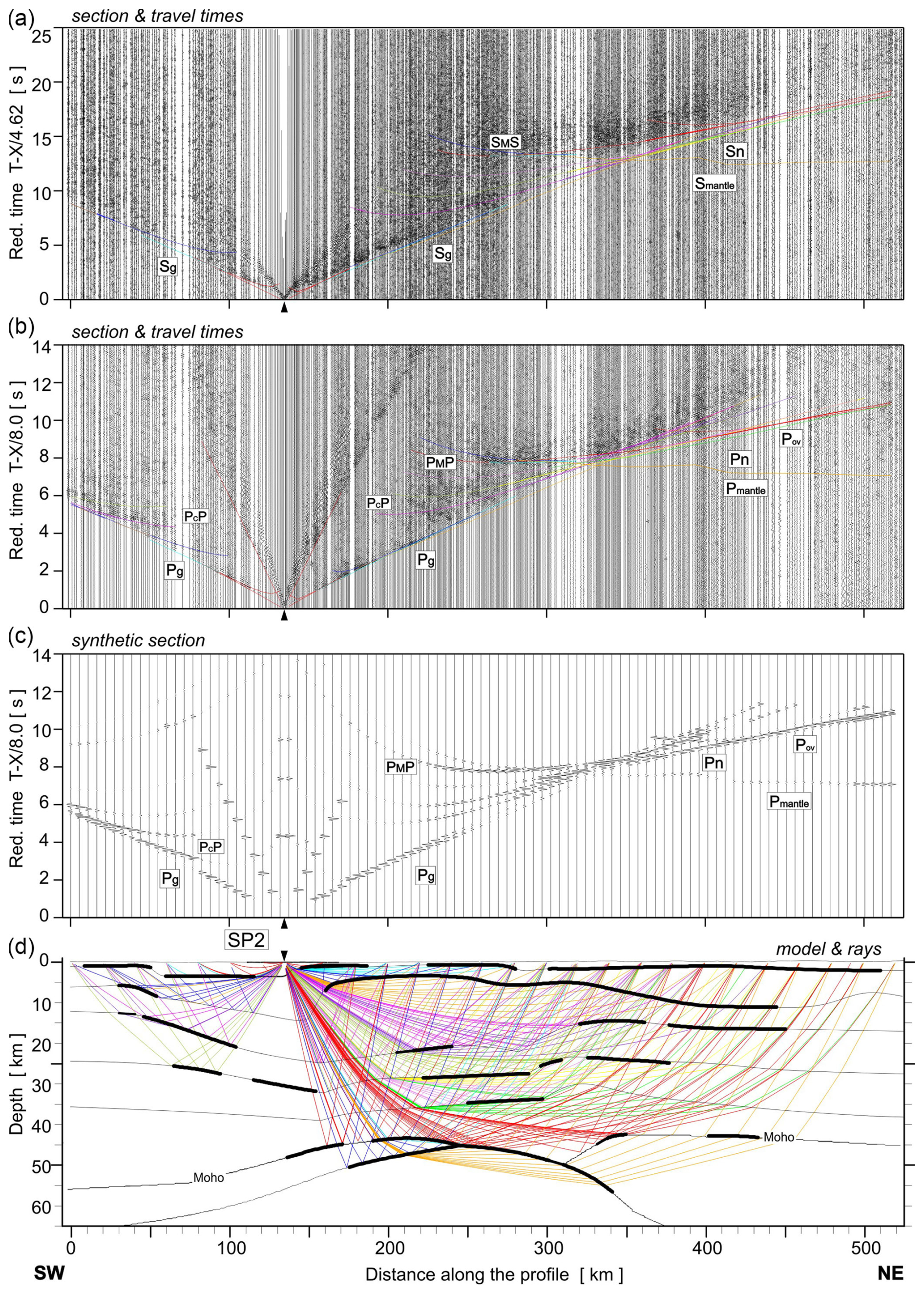
Figure A4 Examples of seismic modelling along the UPPLAND profile, for SP2; seismic record sections (amplitude-normalised vertical component) of S and P wave with theoretical travel times calculated using the SEIS83 ray-tracing technique. (a) For S-wave, we used the band-pass filter of 1–12 Hz and the reduction velocity of 4.62 km s⁻¹. (b) P-wave data have been filtered using the band-pass filter of 2–15 Hz and displayed using the reduction velocity of 8.0 km s⁻¹ for P wave. (c) Synthetic seismograms and (d) ray diagram of selected rays of P wave. All examples were calculated for the models presented in Fig. 4 (main part). Other abbreviations are as in Fig. A1.

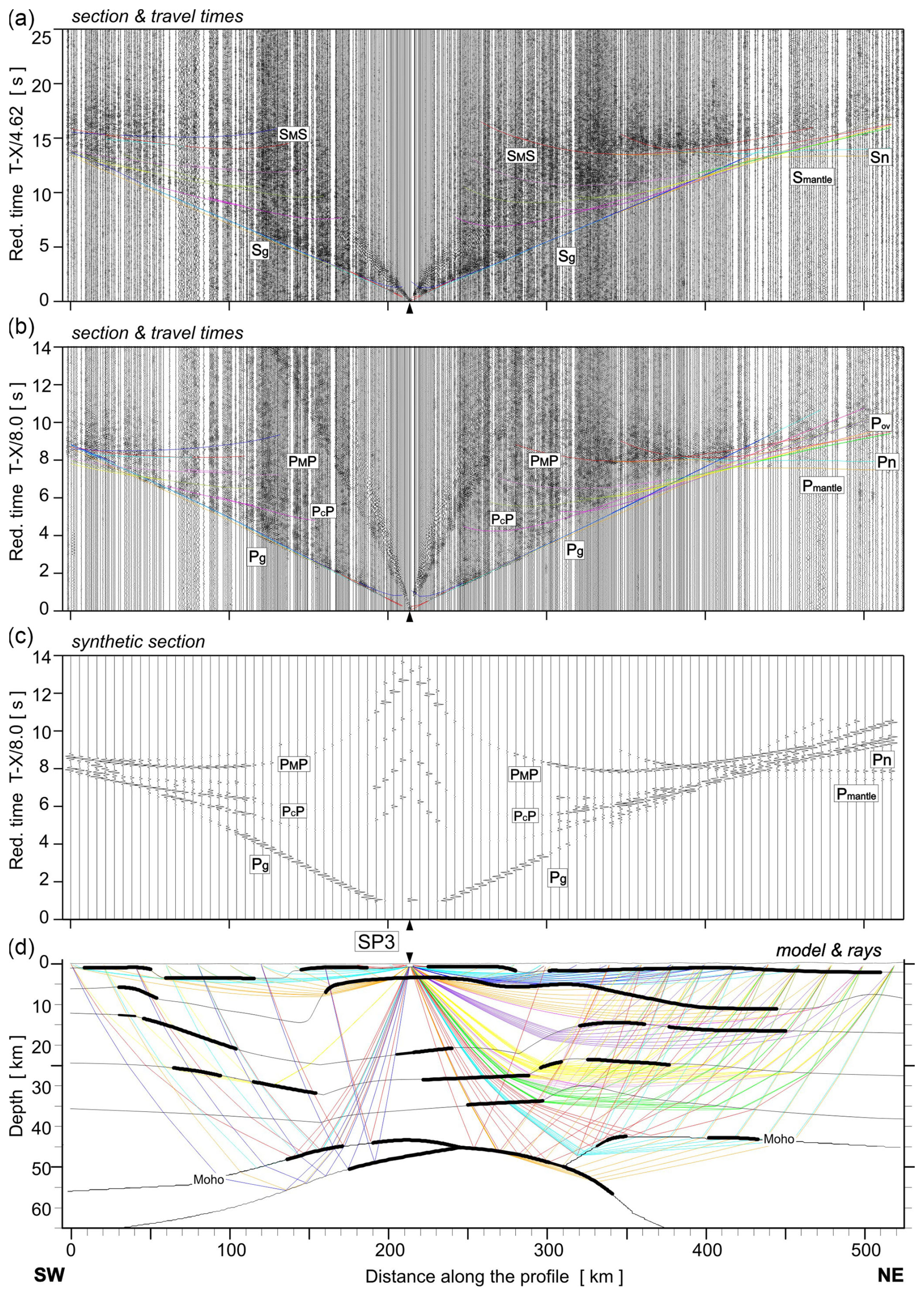
Figure A5 Examples of seismic modelling along the UPPLAND profile, for SP3. Other abbreviations are as in Fig. A4.

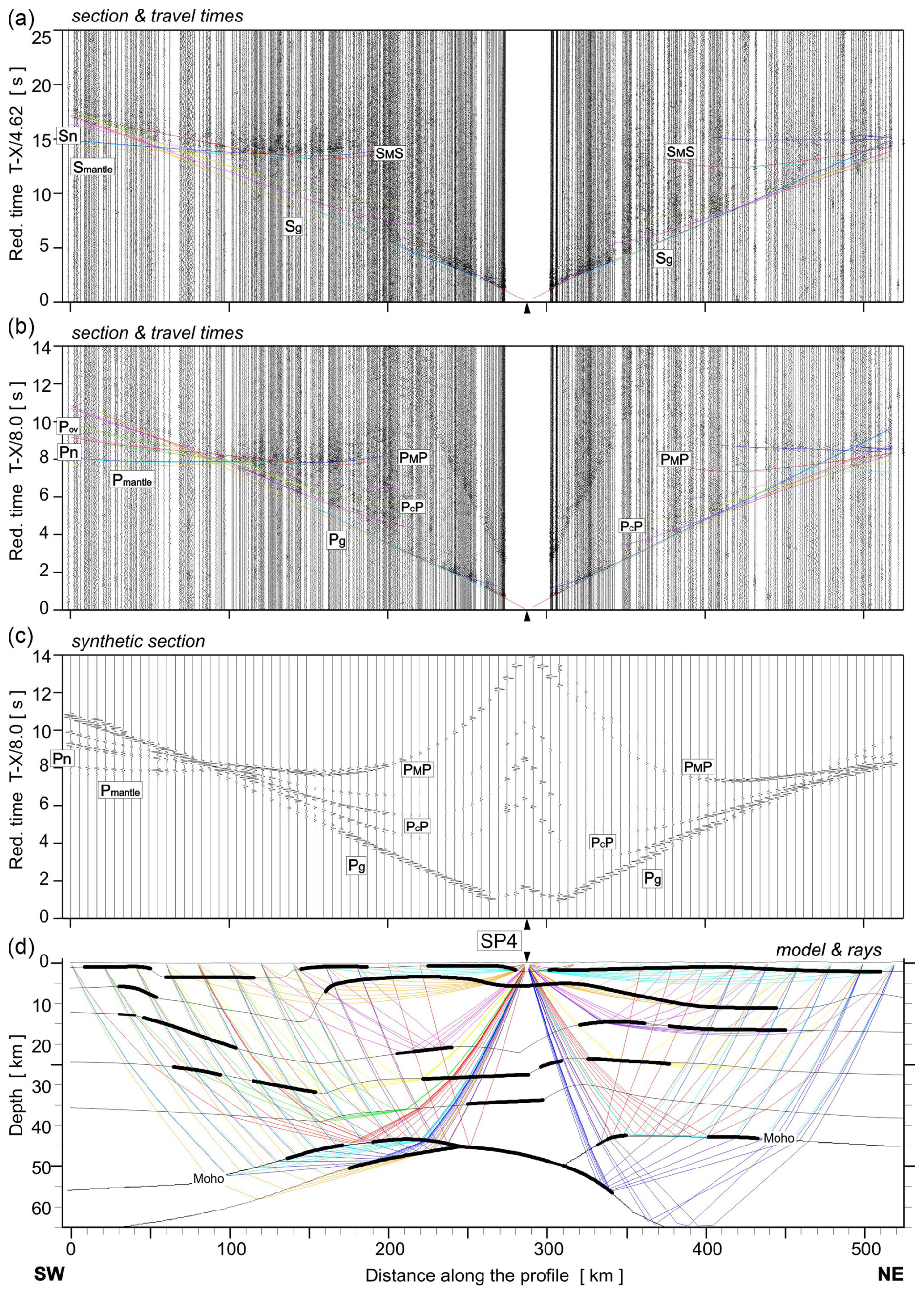
Figure A6 Examples of seismic modelling along the UPPLAND profile, for SP4. Other abbreviations are as in Fig. A4.

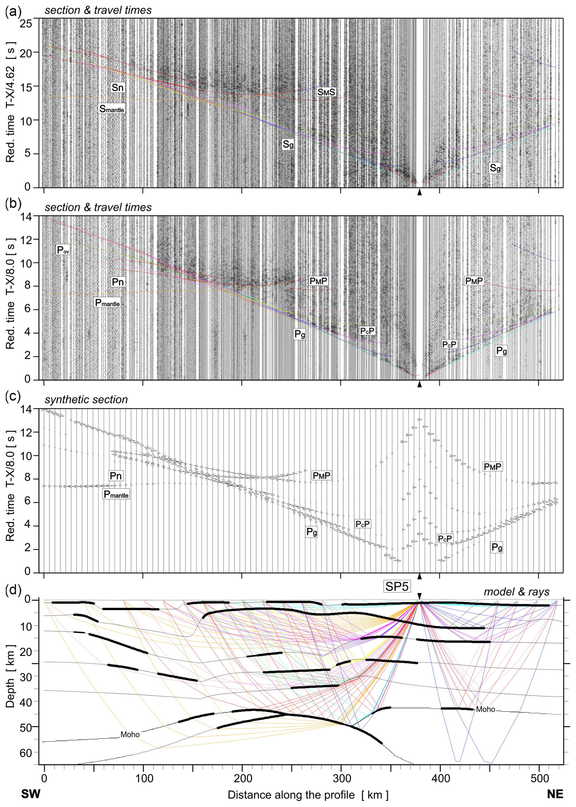
Figure A7 Examples of seismic modelling along the UPPLAND profile, for SP5. Other abbreviations are as in Fig. A4.

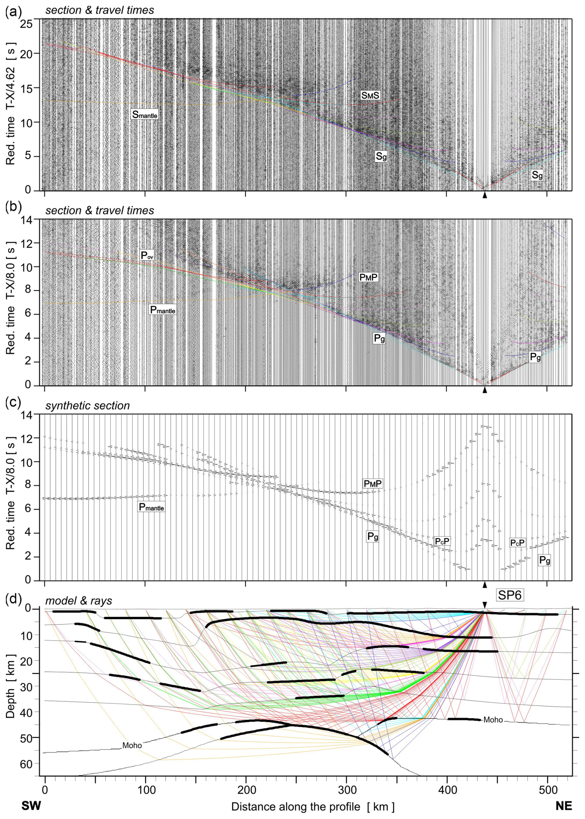
Figure A8 Examples of seismic modelling along the UPPLAND profile, for SP6. Other abbreviations are as in Fig. A4.

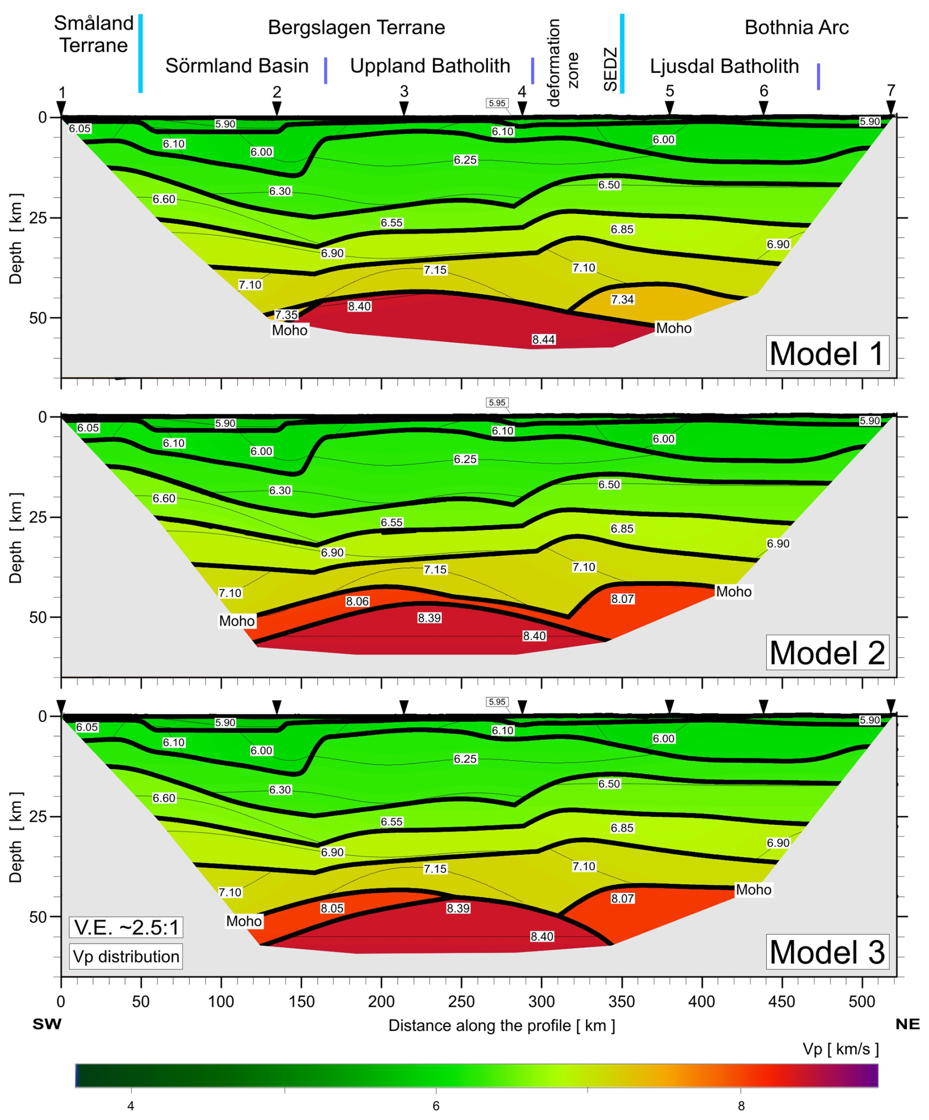
Figure A9 Tests for 3 models (Model 1, Model 2, and Model 3) differing in boundary geometry and velocities in LC and UM (differences described in the text). 2D P-wave velocity model derived by forward ray-tracing modelling using the SEIS83 package (Červený and Pšenčík, 1984) along the UPPLAND profile. Thick black lines represent major velocity discontinuities (interfaces). Thin lines represent velocity isolines with values (in km s⁻¹) shown in white boxes. The position of large-scale crustal blocks is indicated (after Buntin et al., 2021). Arrows show the positions of shot points. Vertical exaggeration is ∼ 2.5:1 for the models.

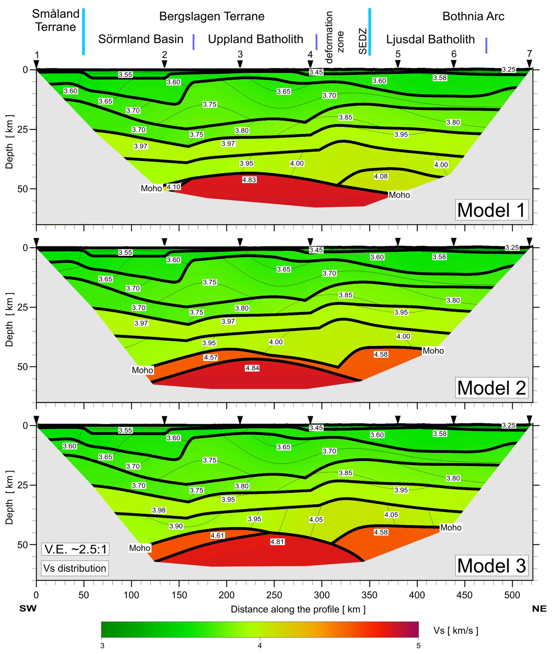
Figure A10 Tests for 3 models (Model 1, Model 2, and Model 3) differing in boundary geometry and velocities in LC and UM (differences described in the text). 2D S-wave velocity models. Other abbreviations are as in Fig. A9.

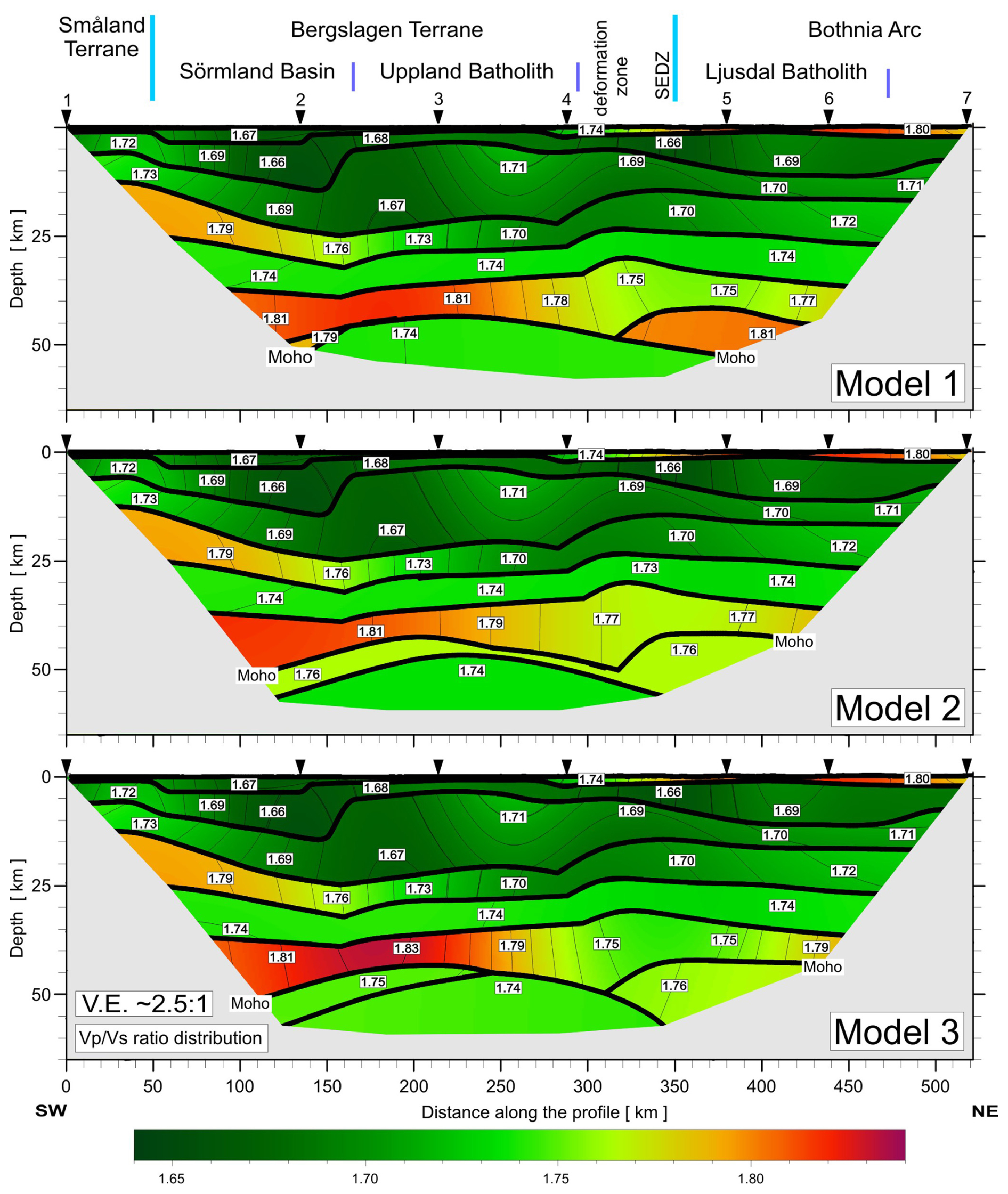
Figure A11 Tests for 3 models (Model 1, Model 2, and Model 3) differing in boundary geometry and velocities in LC and UM (differences described in the text). 2D models of $V_{\mathrm{p}}/V_{\mathrm{s}}$ ratio distribution. Other abbreviations are as in Fig. A9.

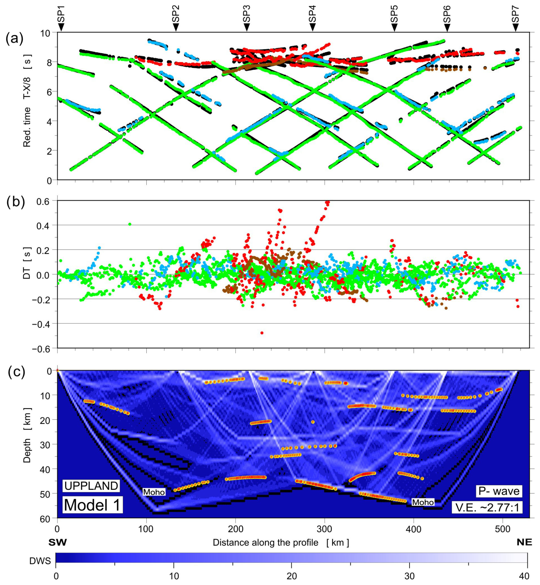
Figure A12 Model 1: diagrams showing theoretical and observed travel times (a), travel time residuals (b), and schematic ray coverage (c) from forward modelling along the profile. Green points – P_g arrivals; blue points – P_cP arrivals (reflections in the crust without P_MP); red points – P_MP arrivals; brown points – P_n arrivals; black points – theoretical travel times; yellow lines – schematic fragments of discontinuities constrained by reflected phases for P-wave velocity Model 1. The red points plotted along the interfaces mark the theoretical bottoming points of reflected phases (every third point is plotted), and their density is a measure of the positioning accuracy of the reflectors. DWS – derivative weight sum. The reduction velocity is 8.0 km s⁻¹.

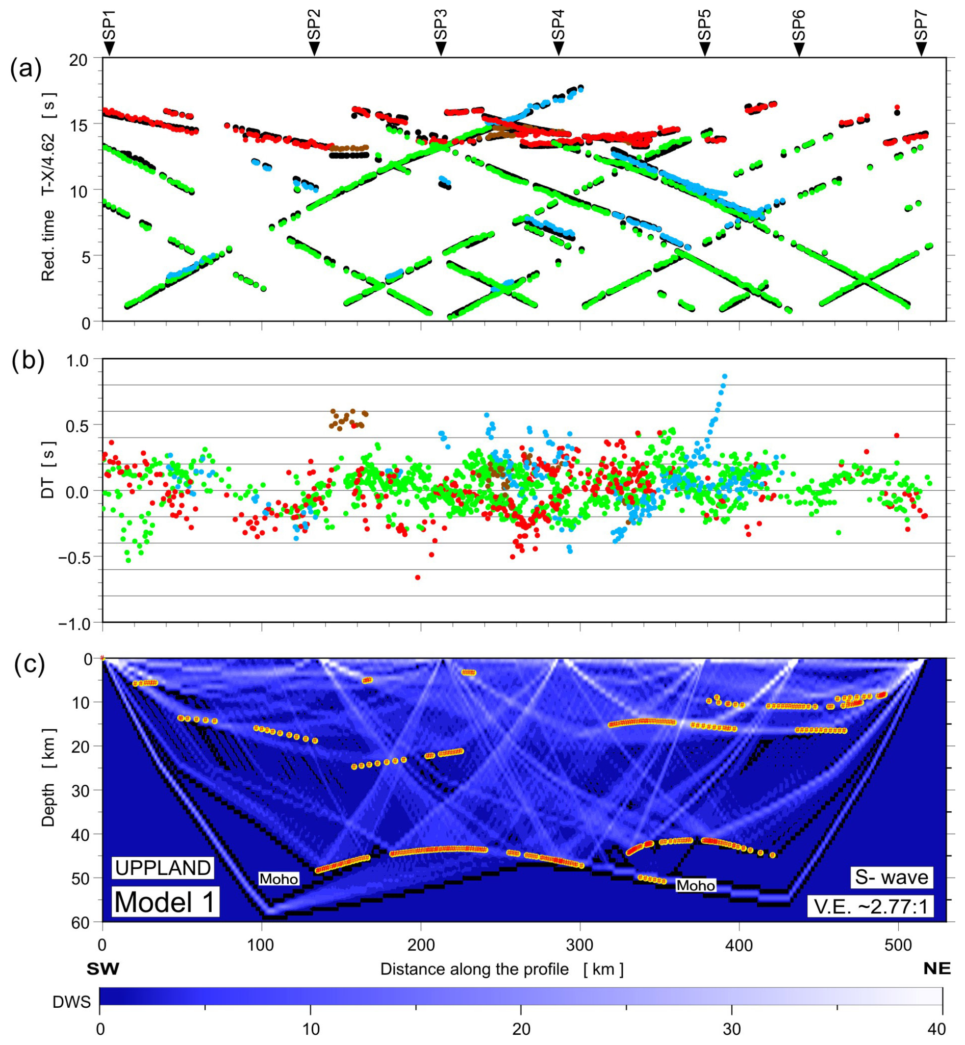
Figure A13 Model 1: diagrams showing theoretical and observed travel times (a), travel time residuals (b), and schematic ray coverage (c) from forward modelling along the profile. Green points – S_g arrivals; blue points – S_cS arrivals (reflections in the crust without S_MS); red points – S_MS arrivals; brown points – S_n arrivals; black points – theoretical travel times; yellow lines – schematic fragments of discontinuities constrained by reflected phases for S-wave velocity Model 1. Other abbreviations are as in Fig. A12. The reduction velocity is 4.62 km s⁻¹.

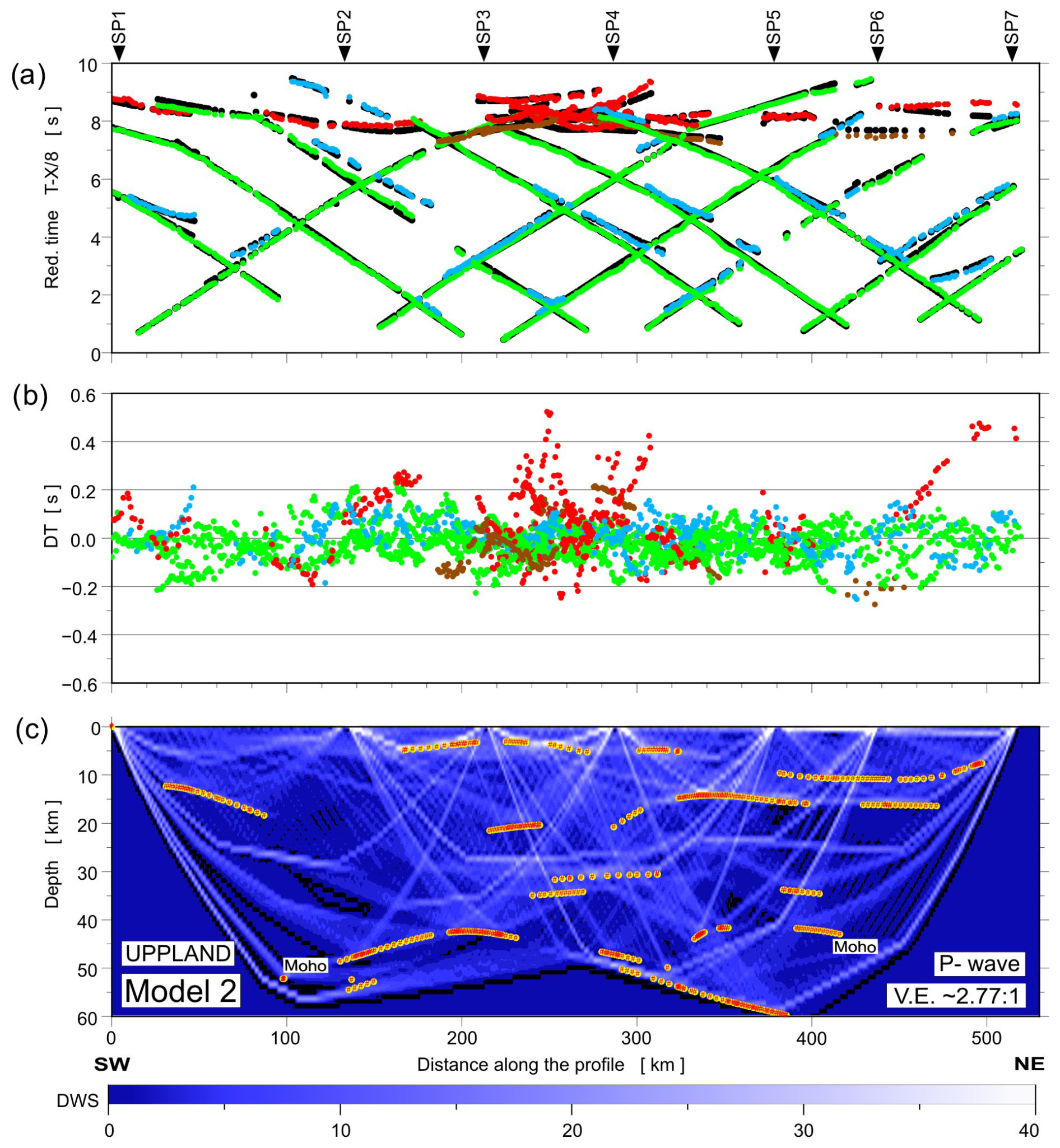
Figure A14 Model 2: diagrams showing theoretical and observed travel times (a), travel time residuals (b), and schematic ray coverage (c) from forward modelling along the profile. Green points – P_g arrivals; blue points – P_cP arrivals (reflections in the crust without P_MP); red points – P_MP arrivals; brown points – P_n arrivals; black points – theoretical travel times; yellow lines – schematic fragments of discontinuities constrained by reflected phases for P-wave velocity Model 2. The red points plotted along the interfaces mark the theoretical bottoming points of reflected phases (every third point is plotted), and their density is a measure of the positioning accuracy of the reflectors. DWS – derivative weight sum. The reduction velocity is 8.0 km s⁻¹.

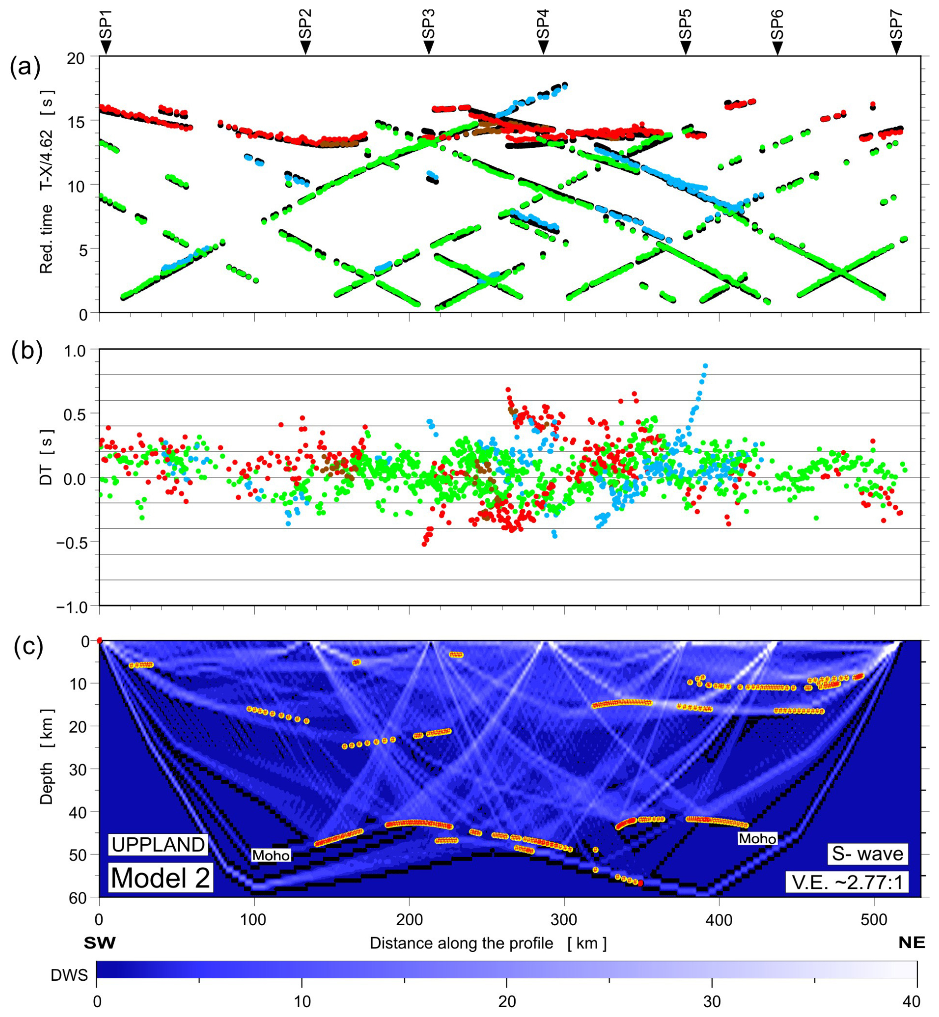
Figure A15 Model 2: diagrams showing theoretical and observed travel times (a), travel time residuals (b), and schematic ray coverage (c) from forward modelling along the profile. Green points – S_g arrivals; blue points – S_cS arrivals (reflections in the crust without S_MS); red points – S_MS arrivals; brown points – S_n arrivals; black points – theoretical travel times; yellow lines – schematic fragments of discontinuities constrained by reflected phases for S-wave velocity Model 2. Other abbreviations are as in Fig. A14. The reduction velocity is 4.62 km s⁻¹.

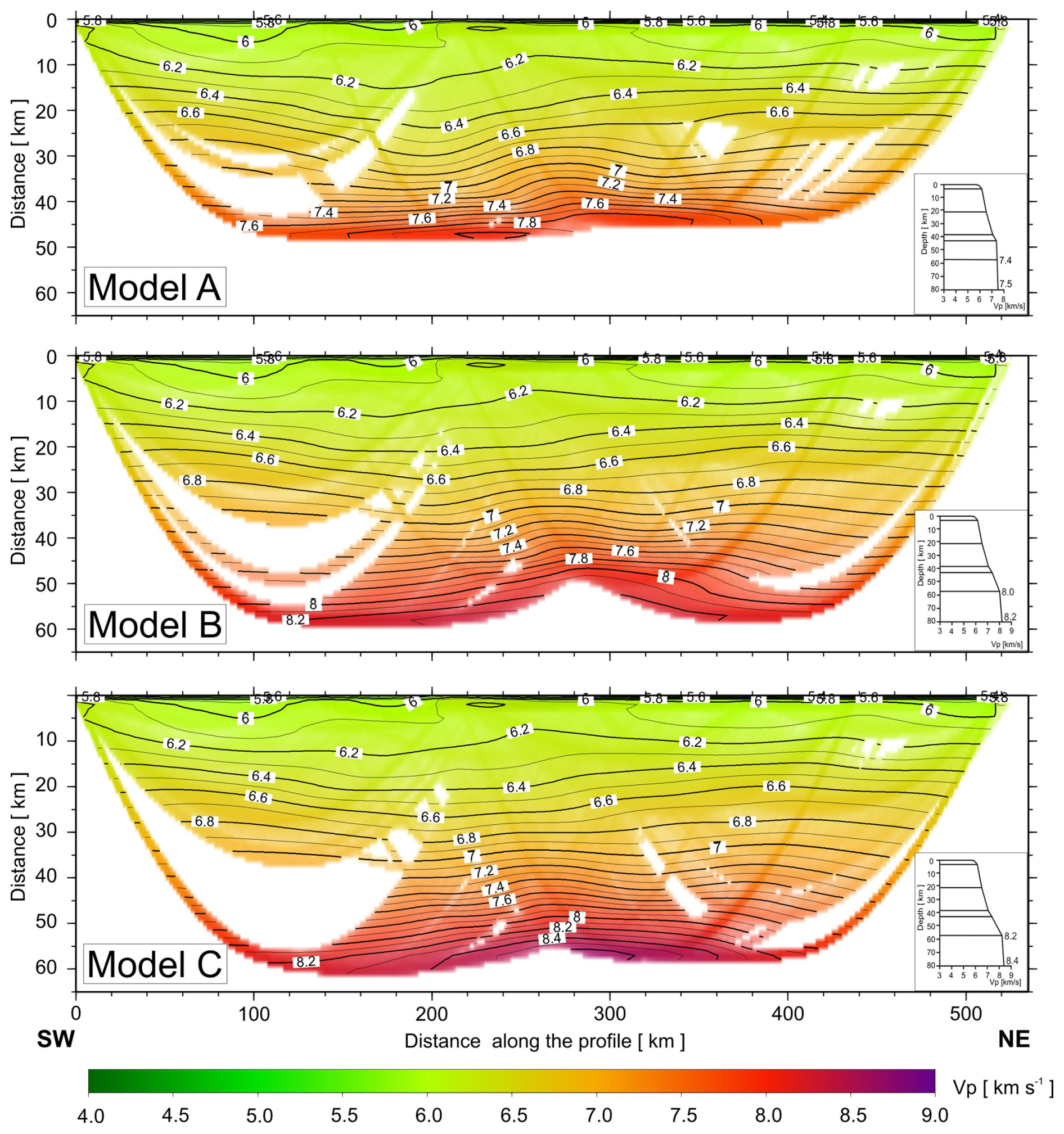
Figure A16 Results of 2D tomographic inversion of P-wave first arrival travel times, obtained using the program package by Hole (1992). Final 2D models for different initial 1D models A, B, and C. Numbers are P-wave velocities (in km s⁻¹).

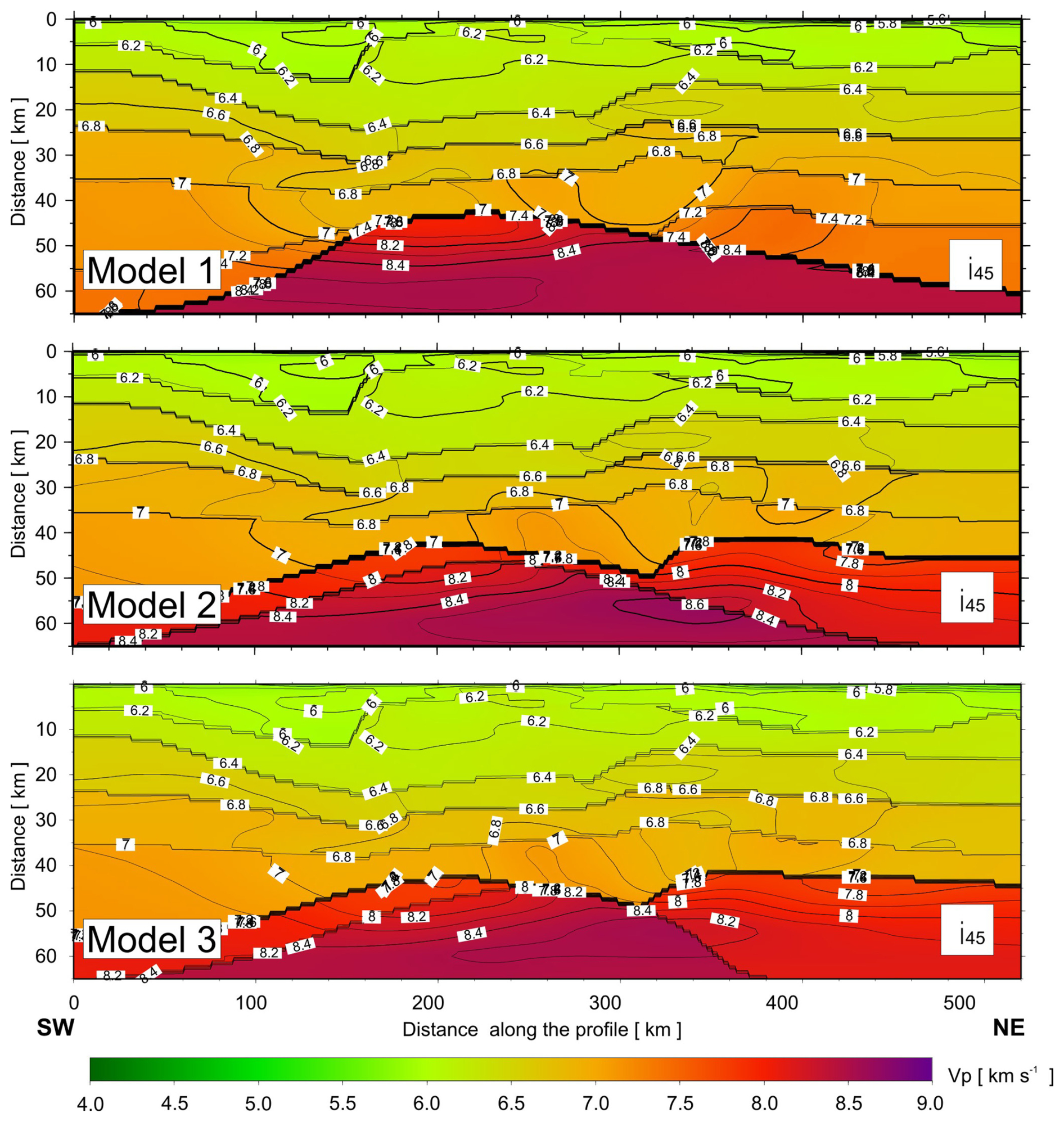
Figure A17 Results of 2D tomographic inversion of P-wave first arrival travel times, obtained using the program package by Hole (1992). 2D models with the final velocity fields obtained using Model 1, Model 2, and Model 3 as initial models and rigid boundary geometry after 45 iterations. Numbers are P-wave velocities (in km s⁻¹).

Table A1 Number of picks with RMS values for each P phase for Model 1.

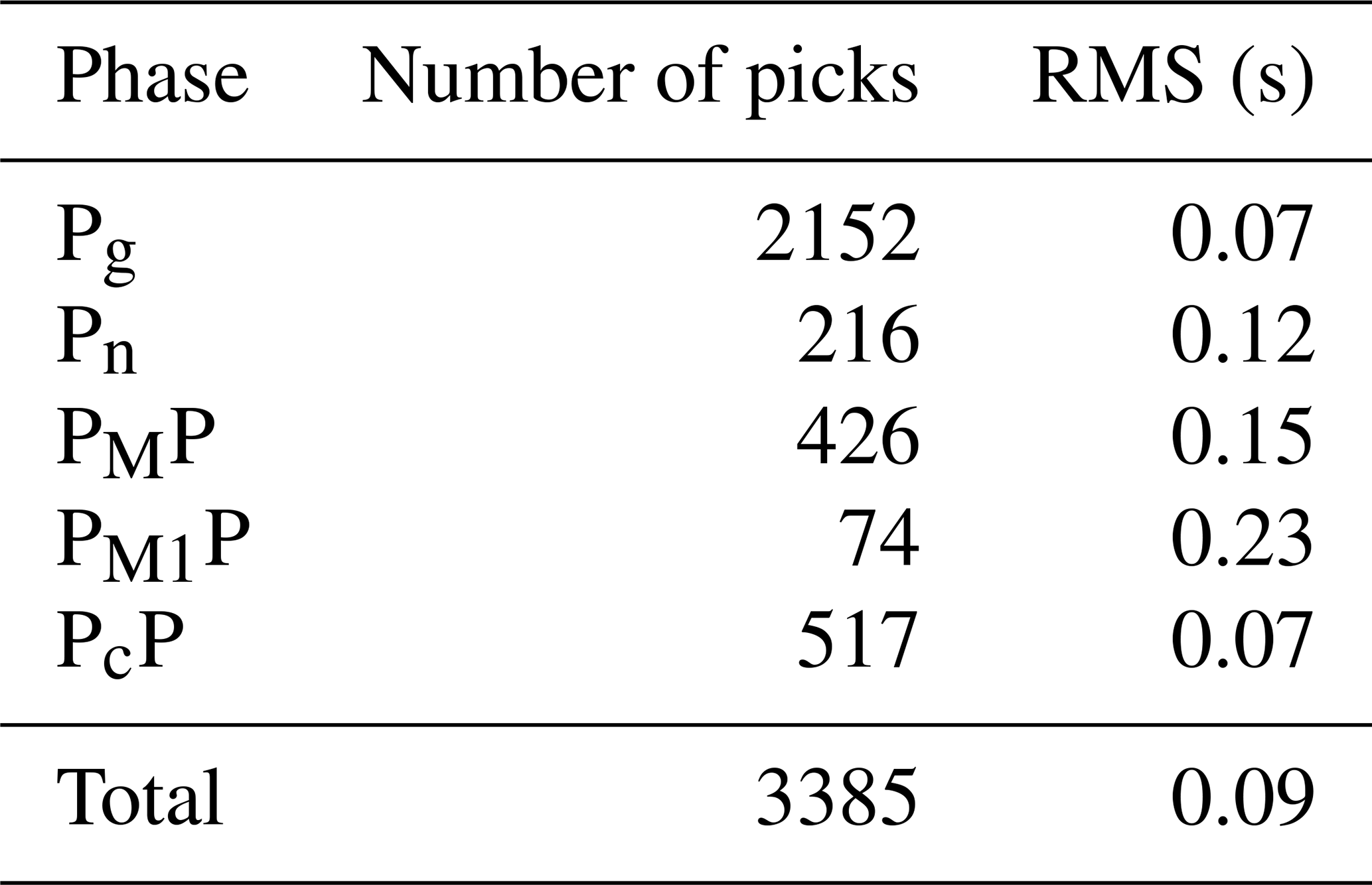
Table A2 Number of picks with RMS values for each P phase for Model 2.

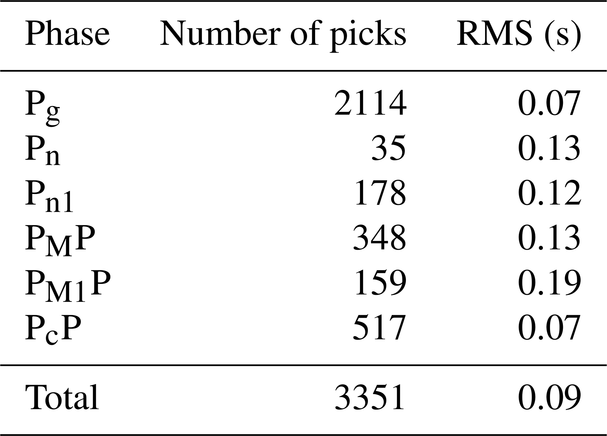
Table A3 Number of picks with RMS values for each P phase for Model 3.

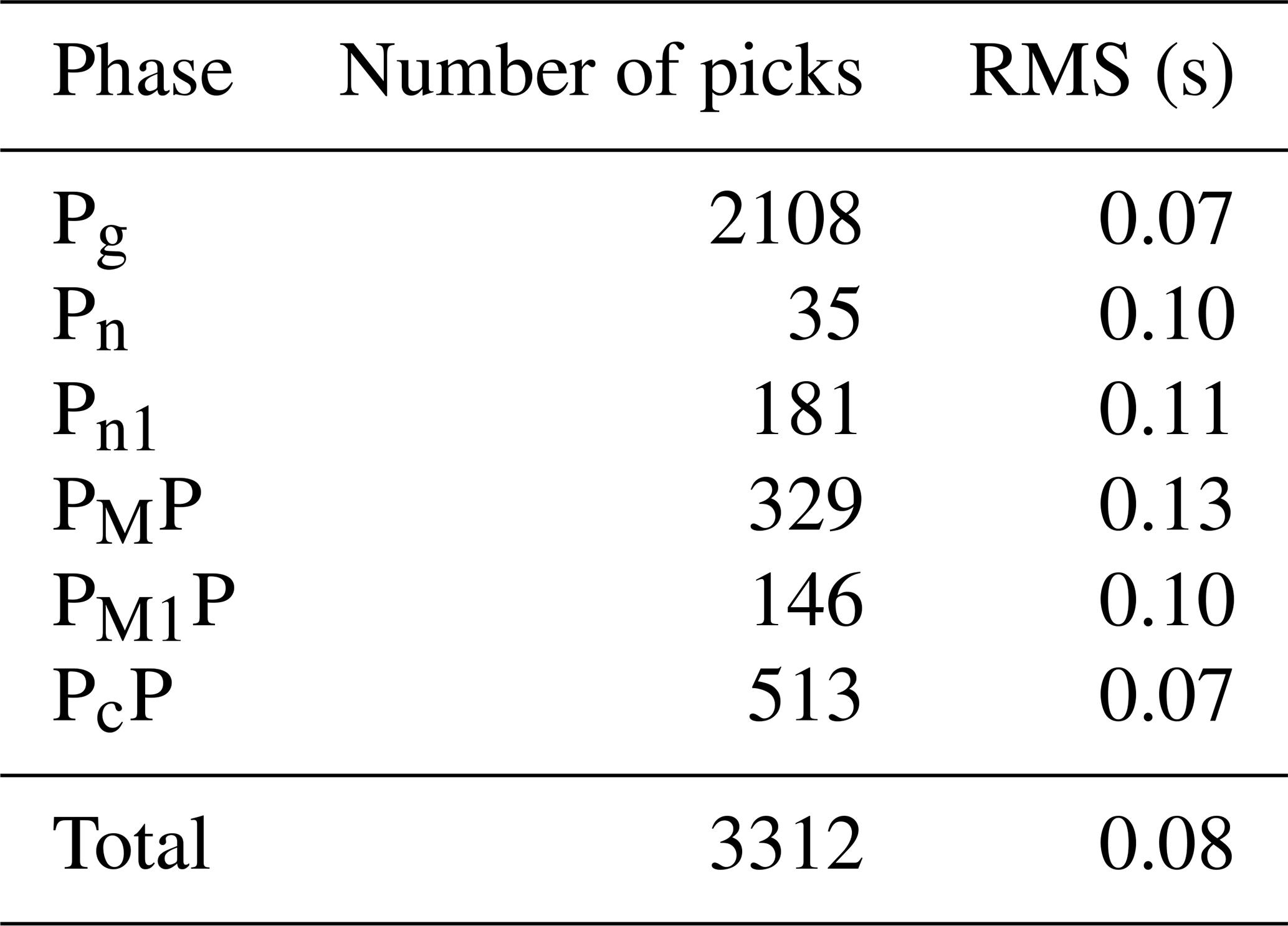
Table A4 Number of picks with RMS values for each S phase for Model 1.

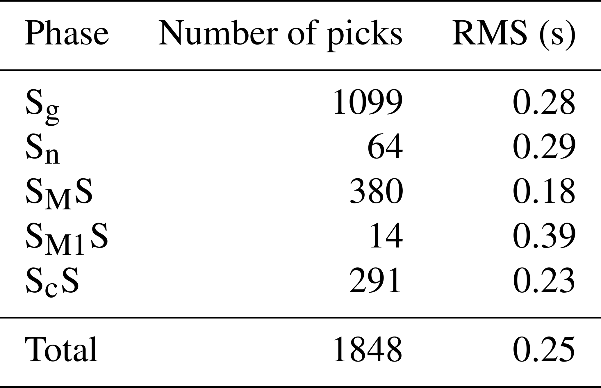
Table A5 Number of picks with RMS values for each S phase for Model 2.

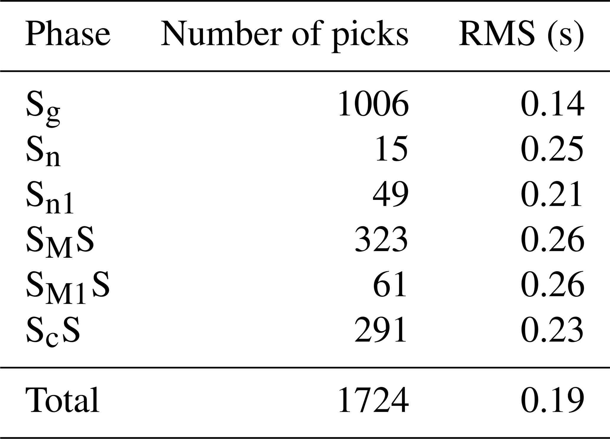
Table A6 Number of picks with RMS values for each S phase for Model 3.

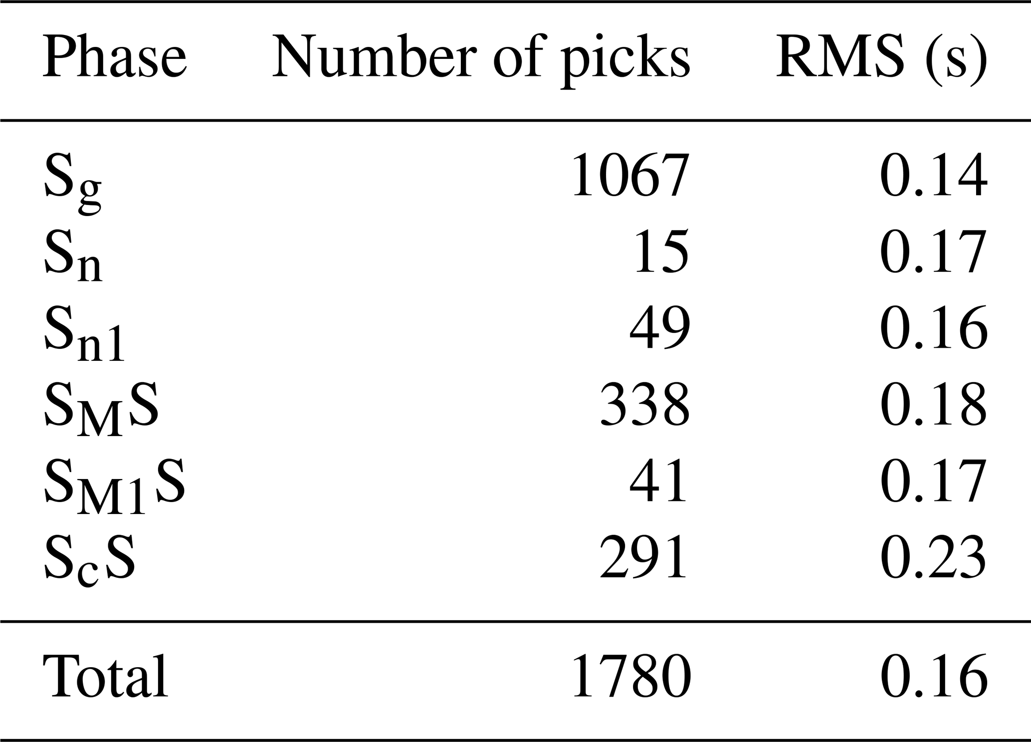
Table A7 RMS values for the analysed models given for starting models 1, 2, and 3 after 10 and 45 (Fig. A7 in Appendix A) iterations.