the Creative Commons Attribution 4.0 License.
the Creative Commons Attribution 4.0 License.
 | 18 Jul 2019
Fault slip envelope: a new parametric investigation tool for fault slip based on geomechanics and 3-D fault geometry
Roger Soliva
Frantz Maerten
Laurent Maerten
Jussi Mattila
By combining a 3-D boundary element model, frictional slip theory, and fast computation method, we propose a new tool to improve fault slip analysis that allows the user to analyze a very large number of scenarios of stress and fault mechanical property variations through space and time. Using both synthetic and real fault system geometries, we analyze a very large number of numerical simulations (125 000) using a fast iterative method to define for the first time macroscopic rupture envelopes for fault systems, referred to as “fault slip envelopes”. Fault slip envelopes are defined using variable friction, cohesion, and stress state, and their shape is directly related to the fault system 3-D geometry and the friction coefficient on fault surfaces. The obtained fault slip envelopes show that very complex fault geometry implies low and isotropic strength of the fault system compared to geometry having limited fault orientations relative to the remote stresses, providing strong strength anisotropy. This technique is applied to the realistic geological conditions of the Olkiluoto high-level nuclear waste repository (Finland). The model results suggest that the Olkiluoto fault system has a better ability to slip under the present-day Andersonian thrust stress regime than for the strike-slip and normal stress regimes expected in the future due to the probable presence of an ice sheet. This new tool allows the user to quantify the anisotropy of strength of 3-D real fault networks as a function of a wide range of possible geological conditions and mechanical properties. This can be useful to define the most conservative fault slip hazard case or to account for potential uncertainties in the input data for slip. This technique therefore applies to earthquake hazard studies, geological storage, geothermal resources along faults, and fault leaks or seals in geological reservoirs.
- Article
(6564 KB) - Full-text XML
- BibTeX
- EndNote


Better understanding of the mechanical interplay between fault slip, 3-D fault geometry, stresses, and rock mechanical properties (e.g. Byerlee, 1978; Morris et al., 1996; Lisle and Srivastava, 2004; Moeck et al., 2009) is an actual and future scientific challenge in geosciences because (1) conventional failure or plasticity laws derived from rock testing does not apply to large rock volumes at geological conditions and timescale (e.g. Brantut et al., 2013) and (2) because fault slip has increasing societal applications (e.g. slip hazard; seismicity; hydraulic fracturing; fault mechanical seal; rock stability; unconventional resources; and storage of hydrocarbon gases, CO2, and compressed air).
Although general knowledge on the geometry, constitution, and behavior of fault zones is improving (e.g. Holdsworth, 2004; Faulkner et al., 2006; Wibberley et al., 2008), it is clear that the large-scale strength of a faulted rock volume is poorly known (e.g. Colettini et al., 2009; McLaskey et al., 2012). Laboratory tests on sampled rocks or fault rocks partly resolve this problem in giving a range of mechanical properties and friction laws. The strength of rocks has been classified under several types of behavior defined by rupture or plasticity envelopes with respect to rock type (Mohr–Coulomb, Byerlee, Griffith, Cam Clay types), which describe typically the elastic domains of small, intact or precut rock samples (Byerlee, 1978; Rutter and Glover, 2012). For pre-existing fault surfaces, fault stability is generally described by the Mohr–Coulomb theory, in which the shear strength (τ) of a fault surface depends on the amount of static friction (μ), the normal stress (σn), and cohesion (Co) on this surface (e.g. Scholz, 2019):
On a simple-planar fault surface, static friction and cohesion define the deviatoric and normal stresses to be applied for fault reactivation (Byerlee, 1978), here referred to as “fault slip”. However, as a result of multistage plate tectonic motions and rock heterogeneity in the Earth's crust, both intraplate and interplate crustal rocks are affected by multiple fracture and fault systems able to slip (e.g. Townend and Zoback, 2000; Anderson et al., 2003), which are more or less complex in their organization on a wide range of scales (isolated, segmented, listric, restricted, branching, intersecting; e.g. Marrett and Allmendinger, 1990; Nicol et al., 1996; Karlstrom and Williams, 1998; Kattenhorn and Pollard, 2001; Soliva et al., 2008). Realistic geometries of faults necessarily imply variations in the shear and normal stresses resolved on the fault surfaces and consequent anisotropy of strength. This concerns the strength of potentially large rock volumes containing faults, governed by their 3-D geometry, stress state, and frictional behavior, for which the value and anisotropy of strength is still a challenge to quantify.
Slip tendency analysis is a well-known method providing tools considering the ratio of resolved shear to normal stresses to model the likelihood for slip on pre-existing surfaces of all possible orientations relative to a regional stress field (e.g. Arthaud, 1969; Morris et al., 1996; Lisle and Srivastava, 2004; Collettini and Trippetta, 2007; Lejri et al., 2017). Beyond its successful application to many cases of fault slip hazard or induced seismicity (e.g. Moeck et al., 2009; Yukutake et al., 2015), this method does not provide the possibility to analyze together large numbers of geological conditions such as variations in stress state, orientation, friction, cohesion, or fluid pressure. Fault slip hazard has generally to be analyzed thoroughly with respect to potential variation through space and time of such important parameters, which actually requires full and time-consuming parametric modeling, and therefore fast calculation techniques. Such a development is, however, critically needed in the new age of data science and numerical geology featured by an increasing availability of 3-D numerical fault system data, in situ rock properties, stress measurements, and high-speed computers. It is also a way to account for potential uncertainties in the input data and to define the most conservative fault slip hazard case.
An improvement of the slip tendency analysis tool, or other equivalent numerical method (Neves et al., 2009; Alvarez del Castillo et al., 2017), would be to incorporate a 3-D mechanical model, allowing the user to analyze the DFN (discrete fault or fracture network) subjected to multiple cases of stress states, and in which fault strength is resolved using a complete static frictional behavior (including cohesion). Although well accepted, Mohr–Coulomb theory has been recently regarded more critically to explain fault initiation under polyaxial loading or in situations where σ2 is not parallel to a pre-existing fault (Healy et al., 2015; Hackston and Rutter, 2016). This fault initiation process, which probably relies more on 3-D stress perturbation around the first initiated faults or pre-existing defect (e.g. Crider and Pollard, 1998; Kattenhorn et al., 2000; Maerten et al., 2002; also see Olson and Pollard, 1991, for a critical analysis of the Coulomb theory for fault initiation), does not discredit the applicability of the Coulomb theory on reactivation of pre-existing fault surface and stress magnitude at failure (Reches and Dieterich, 1983). It can, however, justify the need to consider friction as a potential variable in a wider range than provided by common triaxial test data. Any attempt to quantify the strength of fault systems therefore depends on the development of models coupling pre-existing 3-D fault geometry with both variable fault mechanical properties and triaxial loading conditions through space and time.
In this paper, we use a 3-D boundary element numerical model (iBem3D; e.g. Maerten et al., 2014) in which a Coulomb frictional law is resolved on DFN surfaces to quantify fault system static strength as a function of variable mechanical parameters in a range consistent with geological conditions, and to assess zones having potential for fault slip. Using a fast-calculation iterative method allowing the user to analyze a very large number of numerical simulations (125 000), we define macroscopic fault slip envelopes of rock volumes containing faults as a function of variable stress orientation, 3-D fault geometry and frictional properties. This technique, applied to the case study of the Olkiluoto fault system, allows for analyzing fault-slip hazard for multiple geological scenarios, including variable triaxial stress profiles through space and time and fault mechanical properties in the range of potential uncertainties derived from mechanical tests.
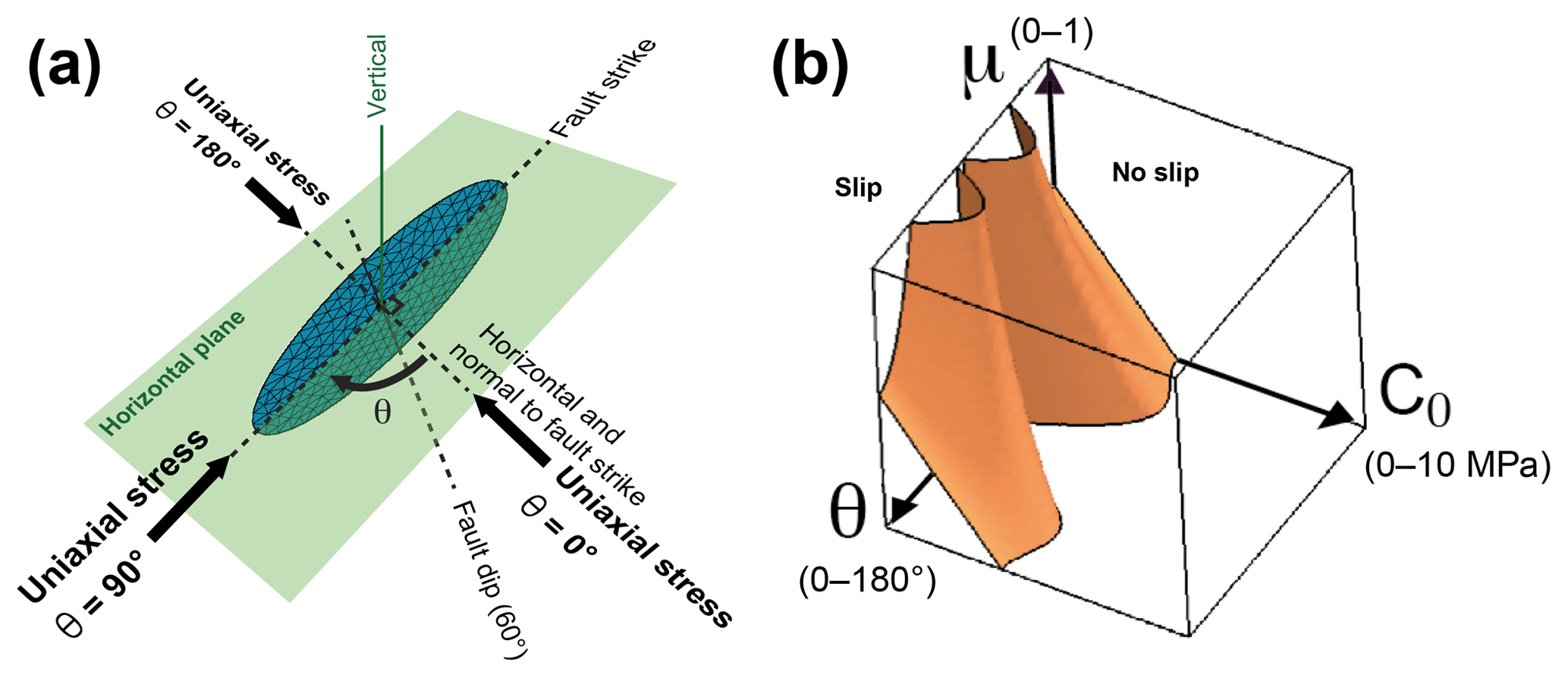
Figure 1Fault slip envelope of a simple-planar elliptical fault of 60∘ dip. (a) Scheme of the relationship between fault strike, dip, and remote uniaxial stress orientation. (b) Fault slip envelope expressed as static friction (μ), cohesion (C0), and uniaxial stress angle (θ). The stable (no slip) and unstable (slip) graphical domains are shown on either side of the fault slip envelope.
2.1 Fault slip envelope setup
We propose to calculate fault slip envelopes for both synthetic and real fault system geometry using the 3-D numerical model iBem3D, a quasi-static iterative boundary element model (Maerten et al., 2014). In iBem3D, faults are discretized using triangulated surfaces of frictional behavior (Eq. 1) in a heterogeneous, isotropic elastic whole- or half-space also allowing mechanical interaction between each triangular element when the fault surfaces slip (Maerten et al., 2002). For the first part of this study aiming to define fault slip envelopes, the effective stress state is simplified as a horizontal simple-uniaxial stress (σ) of 10 MPa with variation in the angle ]∘ with respect to fault orientation. This uniaxial condition allows for highlighting the dependence of fault slip on friction and cohesion under simple stress condition. Modeling using more realistic stress conditions (i.e. in 3-D and evolving with space and time) will be used for the Olkiluoto fault system study (see Sect. 2.2). Static friction and cohesion values, as measured in laboratory rock tests or from deep stress measurements, typically vary in the range of and MPa, respectively (Hatheway and Kiersch, 1989). To analyze the sensitivity of fault slip as a function of these properties and stress orientation (μ, C0, and θ), we use them as variables in the given ranges with 50 values for each parameter. This leads to the analysis of a very large number of models (503=125 000). The computation time has therefore been optimized using the H-Matrix technique parallelized for multi-core CPU architectures. The resulting fault slip envelope separates the parametric domain (μ, C0, and θ) where the fault is unstable (slip) from where the fault is stable (no slip). Also note that fluid pressure, although not considered in this study (see Sect. 4), is considered in iBem3D as an isotropic pressure into the faults that can also be considered a variable.
Fault slip can occur in places where the Coulomb criterion is reached on fault surfaces. In other words, slip occurs along preferred orientations of fault surfaces with respect to the amount of friction, cohesion, and resolved shear and normal stresses on fault planes computed following the Cauchy equations (e.g. Pollard and Fletcher, 2005; Jaeger and Cook, 1979). Quasi-static fault displacement (net slip) can be computed on fault planes using linear elasticity (see Thomas, 1993; Maerten et al., 2010, 2014, 2018; for full explanation), taking into account static friction and cohesion, mechanical interaction due to stress perturbation between faults (e.g. Crider and Pollard, 1998; Kattenhorn et al., 2000; Soliva et al., 2008; Maerten et al., 2014), and using Young's modulus (E) and Poisson's ratio (ν) of 1 GPa and 0.25, respectively. This quasi-static displacement, rather than the coseismic value of displacement which must also be affected by dynamic rupture processes, is considered the fault ability to initiate and accumulate slip along fault.
We studied first a synthetic fault geometry characterized by a 60∘ dip simple-planar elliptical surface such as described for a simple-isolated normal fault (Nicol et al., 1996; Fig. 1a). More complex synthetic geometries were also tested such as intersecting conjugate faults, consistent with normal (60∘ dip), strike-slip (90∘ dip), thrust-fault configurations (30∘ dip), a more complex pattern containing all these configurations (Fig. 2a), or again the case of the sphere (Fig. 2b). Fault slip envelopes have also been calculated on the three real fault system geometries (or DFN) shown in Fig. 3a, b, and c: Landers, Chimney Rock, and Oseberg Syd respectively used in Maerten et al. (2001, 2002), Lovely et al. (2009), and Madden et al. (2013). For the Landers and Chimney Rock cases, the 3-D fault surfaces were extruded downward from a 2-D trace mapped at the Earth's surface, whereas the Oseberg Syd geometry is derived from a high-quality seismic reflection survey. Uncertainty about 3-D fault geometry discretization is not accounted for in this study (see the discussion in Sect. 4). For these three fault system configurations, the uniaxial stress orientation, θ=0∘, corresponds to the west, θ=90∘ to the north, and θ=180∘ to the east. The aim is therefore not to provide a geologically plausible study (as exposed in Sect. 2.2 for the Olkiluoto fault system study) but to illustrate fault slip envelope as a function of fault system complexity using realistic fault geometry.

Figure 2Synthetic 3-D fault geometries and their fault slip envelopes. (a) Variable 3-D intersecting fault geometries and related fault slip envelope calculated with the same variables as Fig. 1. (b) Theoretical case of a sphere and its fault slip envelope calculated with the same variables as (a) and Fig. 1. The small empty box indicates the parameters on each axis of the envelope diagrams shown in panels (a) and (b).
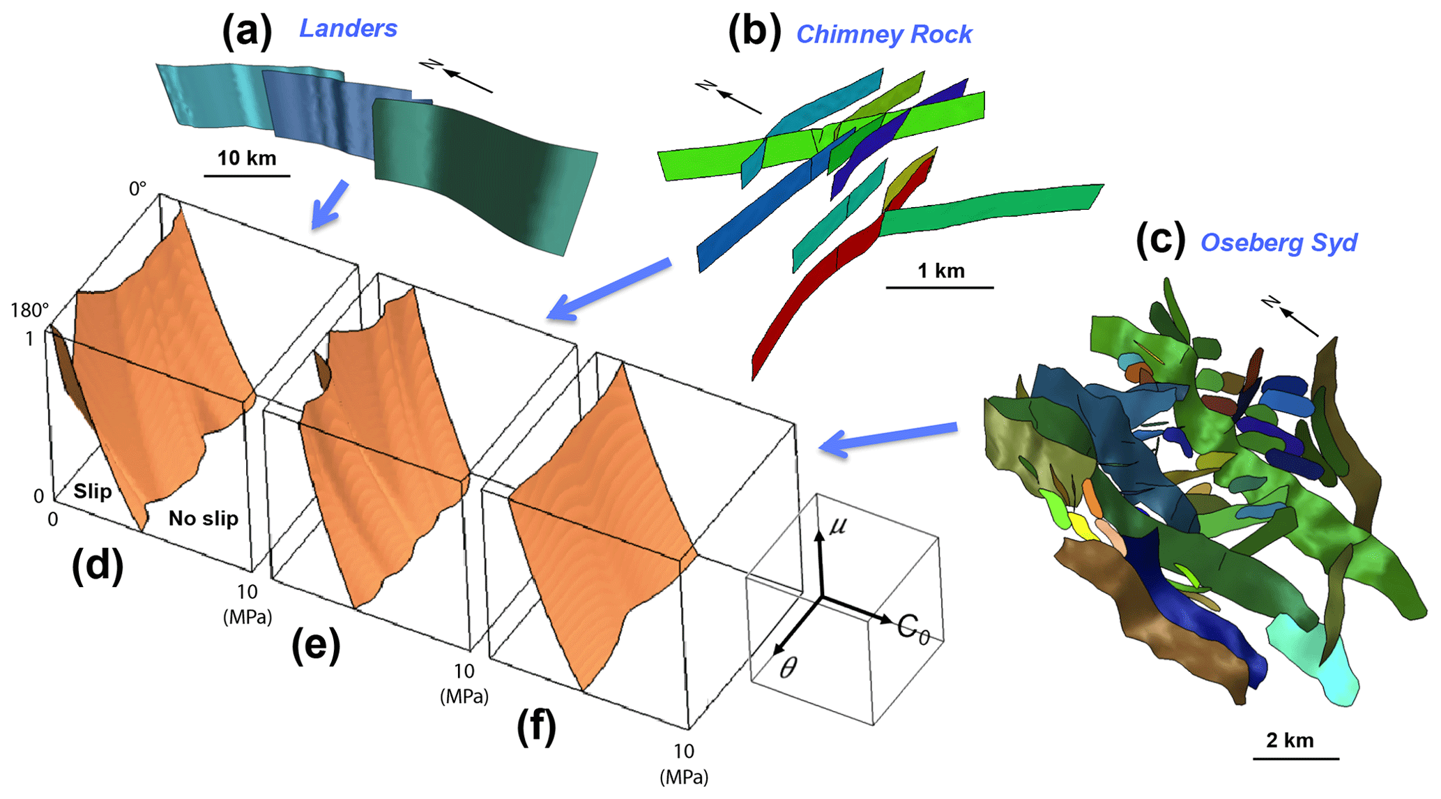
Figure 3Examples of 3-D fault system geometry from a simple to a very complex case, and related fault slip envelopes. (a) The Landers strike-slip fault segments. (b) The Chimney Rock conjugate strike-slip fault system. (c) The Oseberg Syd normal fault system. Panels (d), (e), and (f) are fault slip envelopes for each fault system, defining fault system stability for variable uniaxial stress orientation (θ), static friction (μ), and cohesion (C0) on fault surfaces. Colors in (a), (b), and (c) correspond to different fault surfaces and allow an individual fault to be identified.
2.2 Parametric study of the Olkiluoto fault system
We apply this technique to study the potential of fault reactivation in the fault system of Olkiluoto Island (Finland), where a deep geological high-level nuclear waste repository is being built and which also is a site for two operational nuclear power plants. The site is located in Paleoproterozoic amphibolite-facies metasedimentary rocks and tonalitic-granodioritic-granitic gneisses, cut by a complex 3-D geometry of brittle faults, spanning in age from 1.7 to 1.0 Ga, and formed during several different tectonic episodes (Mattila and Viola, 2014). It is thought that these faults may be subjected to reactivation in a future glacial cycle (120 kyr from now) due to the loading–unloading effect of a glacial ice sheet cover. Such an event is evidenced by prominent postglacial faults observed in northern Scandinavia, known to have occurred at the retreating phase of the last glaciation (Arvidsson, 1993). The stress state evolution due to this ice sheet cover is expected to be the major change in loading conditions of the fault system surrounding the Olkiluoto site and northern Europe in general.
The present-day stress state (Fig. 6a, 0 m of ice), the 3-D shape of this fault system (Fig. 6b), and the rock mechanical properties have been thoroughly inspected in the area from the 1980s to the present day and are used to constrain our modeling. The DFN geometry has been defined by 3-D and 2-D seismic surveys and cross-hole data correlation of a total of 57 measurements at diamond-cored boreholes and the underground characterization facility, reaching the depth of 450 m (Aaltonen et al., 2010). This fault system, which extends at least to the depth of 2 km, is used in our simulation as a relevant example of real 3-D fault system complexity in a highly important area. A fine discretization of the fault surfaces with triangular elements representing less than a hundred meters in length allows the use of high-accuracy fault geometry as required to study fault slip and mechanical interaction.
Based on present-day stresses (σH is E–W) and elastic rock properties (E=55 GPa and ν=0.25) (see Sjöberg, 2003; Hakkala et al., 2013) we approximate realistic stress boundary conditions in considering the presence of a future glacial ice sheet. Because in geological conditions principal stress axes are subjected to permutations through time and space, such an approach gives the opportunity to see geologically consistent effects of changing stress magnitudes, Andersonian regime (i.e. σv=σ1, σv=σ2, or σv=σ3), and the relative angle between the stresses and the faults (θ). Since lithosphere flexural stresses or stress earthquake triggering are difficult to define, it is worth considering principal stresses as variable parameters in a lower end-member case scenario. The presence of an ice sheet in the area will at least increase the vertical load due to its increase in thickness. Based on climate models and previous studies of the past glacial events (Skinner and Porter, 1987; Berger and Loutre, 1997), the ice sheet is expected to vary from 0 up to 2.5 km thickness above the faults during the next 120 kyr, with a maximum thickness reached at 100 kyr from nowadays. The subsequent stress state into the rock mass is calculated from the measured present-day stress field (overcoring and hydraulic fracturing; Ask, 2011) and additional vertical and confining stresses due to the ice thickness.
We calculated the triaxial stress profiles due to an increase in vertical load and its subsequent confining pressure such as
in which σV, σH, and σh are respectively the vertical, maximum horizontal, and minimum horizontal stresses; σV0 is the lithostatic stress; σVice the vertical load due to the ice thickness; and TcH and Tch are the major and minor tectonic constants applied horizontally, respectively. σV0 and σVice are calculated along depth profiles as a function of the material density and the thickness of each unit. The tectonic constants are calculated as the difference between the measured actual in situ horizontal stresses and the confining pressure due to the vertical lithostatic load:
We, however, note that the stresses above a depth of 300 m are not precise (Ask, 2011) probably because they are too close to the surface where the in situ stresses are estimated to be perturbed. The present-day tectonic constant profiles have been extracted (from Eqs. 3 and 4). They increase linearly with depth and are interpreted to be due to the Atlantic ridge push (Forsyth and Uyeda, 1975; Grollimund and Zoback, 2000), and are therefore assumed to be constant during the next glacial cycle.
Stress permutations are expected due to strong variations in the stress distribution at depth (Fig. 3a). A hybrid thrust-fault and strike-slip regime is measured in the actual conditions with no ice sheet, with a prominent proportion of thrust-fault regime above 1 km in the rock mass. An increasing proportion of the strike-slip regime is calculated with increasing of ice sheet thickness up to 1.5 km. Pure strike-slip regime is expected for ice thicknesses ranging between 1.5 and 2.2 km and a hybrid strike-slip (at depth) to normal-fault regime (shallow) is expected between 2.2 and 2.5 km of ice. These variations in principal-stress profiles through time and space, expressed as ice thickness ∈ [0, 2500] m, will be used as a main variable in the parametric study.
The frictional behavior of the fault zones is also a major process to consider as a variable. Measurements of friction and cohesion values have been done on the Olkiluoto-fault core rocks (Hudson et al., 2008; Mönkkönen et al., 2013). These estimations give effective macroscopic values of static friction in the range of and cohesion in the range of MPa. These estimations give a wide range of values that reflect the large variety of fault rocks observed in dry conditions (breccias, cataclasites, gouges) and for small samples. It is, however, worth noting (i) that wetness and fluid pressure can strongly reduce these values, (ii) that it is impossible to predict in which part of the fault core slip will occur, and (iii) that these measurements (obtained in the tunnel and from drill cores) are for a very limited part of the entire fault surface and do not take into account the integral upscaled effect. We therefore use static friction and cohesion applied to the entire fault system as variables in a wider range comparable to the values used for the first models. Static friction and cohesion vary such as and MPa, respectively.
In the same way as previously shown, 50 values of each variable, i.e. ice thickness, friction, and cohesion, have been chosen and the fault slip envelope obtained for the Olkiluoto Island fault system separates the parametric domain (here μ, C0, and ice thickness) where the faults are unstable (slip) from the domain where the faults are stable (no slip).
3.1 Fault slip envelope
The fault slip envelope for a simple-elliptical fault (Fig. 1) appears mainly sinuous in shape in the direction of θ. Figure 1a shows the model geometric conditions between θ, fault strike, fault dip, and the horizontal uniaxial stress applied for this simple-elliptical fault study (also see Sect. 2.1). Note that when θ=0 or 180∘, the angle between the stress axis and the fault surfaces is 60∘, the fault dip angle. The 3-D geometry of the fault slip envelope (Fig. 1b) shows that slip is favored when the uniaxial stress is oblique to fault strike, and the optimal angle slightly changes with the friction coefficient. Consistent with the Mohr–Coulomb theory, fault slip occurs for a wider range of cohesion when friction is low and conversely for a lower range of cohesion when friction is high. Fault slip appears impeded for two main configurations of resolved shear-stress minima: where the uniaxial stress is parallel to the fault surface (θ=90∘) or where it is normal to fault strike (θ=0 or 180∘). This last configuration, which has an angle of 60∘ between the stress axis and the fault surface, allows fault slip for low friction and impedes slip for high friction.
For more complex fault geometries, the fault slip envelopes are sinuous in the direction of θ, with symmetric polymodal shapes reflecting the geometry of the fault configurations tested (Fig. 2a). The number of modes of fault instability can vary with the friction coefficient, especially in the models containing vertical faults for which variations in θ affect drastically the relative orientation of the uniaxial stress with the fault surface. For the strike-slip configuration, two modes are observed at θ=0 and 90∘ for μ=0 (at 45∘ of each fault surface) and four modes at θ=15, 60, 105 and 165∘ close to μ=0.5 (i.e. uniaxial load at about 30∘ of each fault surface). The complex synthetic model including the conjugate fault configuration altogether presents results that are therefore quite complex in shape but actually do not show strong variations since many fault orientations are represented, and tend to approach the planar shape expected for the case where all the possible fault orientations are represented (see the synthetic case of the sphere, Fig. 2b). We also note that fault slip occurs for a wider range of cohesion when friction is low and for a lower range of cohesion when friction is high.
Similar results can be found for the real fault systems (Fig. 3, see references in Sect. 2.1 for the source data). In simple fault geometry such as the Landers or Chimney Rock examples (Fig. 3a and b), the common segmentation or conjugate geometries frequently found in fault systems provide quite constant fault orientation through space. This therefore results in significant spatial anisotropy of strength, expressed by a local inflection of the fault slip envelope as a function of θ (Fig. 3d and e). In more complex fault systems, such as the Oseberg Syd example (Fig. 3c), there are frequently parts of fault surfaces optimally oriented to slip with respect to stress orientation, implying no significant spatial anisotropy of strength (Fig. 3f).
In both synthetic and real fault system geometries (Figs. 1, 2, and 3), the degree of irregularity of the fault slip envelope appears to be inversely correlated with the degree of orientation anisotropy of the 3-D fault system. The fault slip envelopes appear mainly sinuous in shape in the direction of θ, showing the strong influence of the stress orientation on the shape of the fault slip envelope. Fault slip is favored when the uniaxial stress is oblique to fault strike, and the optimal angle slightly changes with the friction coefficient. Conversely, fault slip is impeded for two main configurations of resolved shear-stress minima: where the uniaxial stress is parallel to the fault surface (e.g. see the main deflection at θ∼155∘ on the envelope in Fig. 3d) or where it is normal to fault strike (θ∼65∘). Also note that fault slip occurs for a wider range of cohesion when friction is low and for a lower range of cohesion when friction is high.
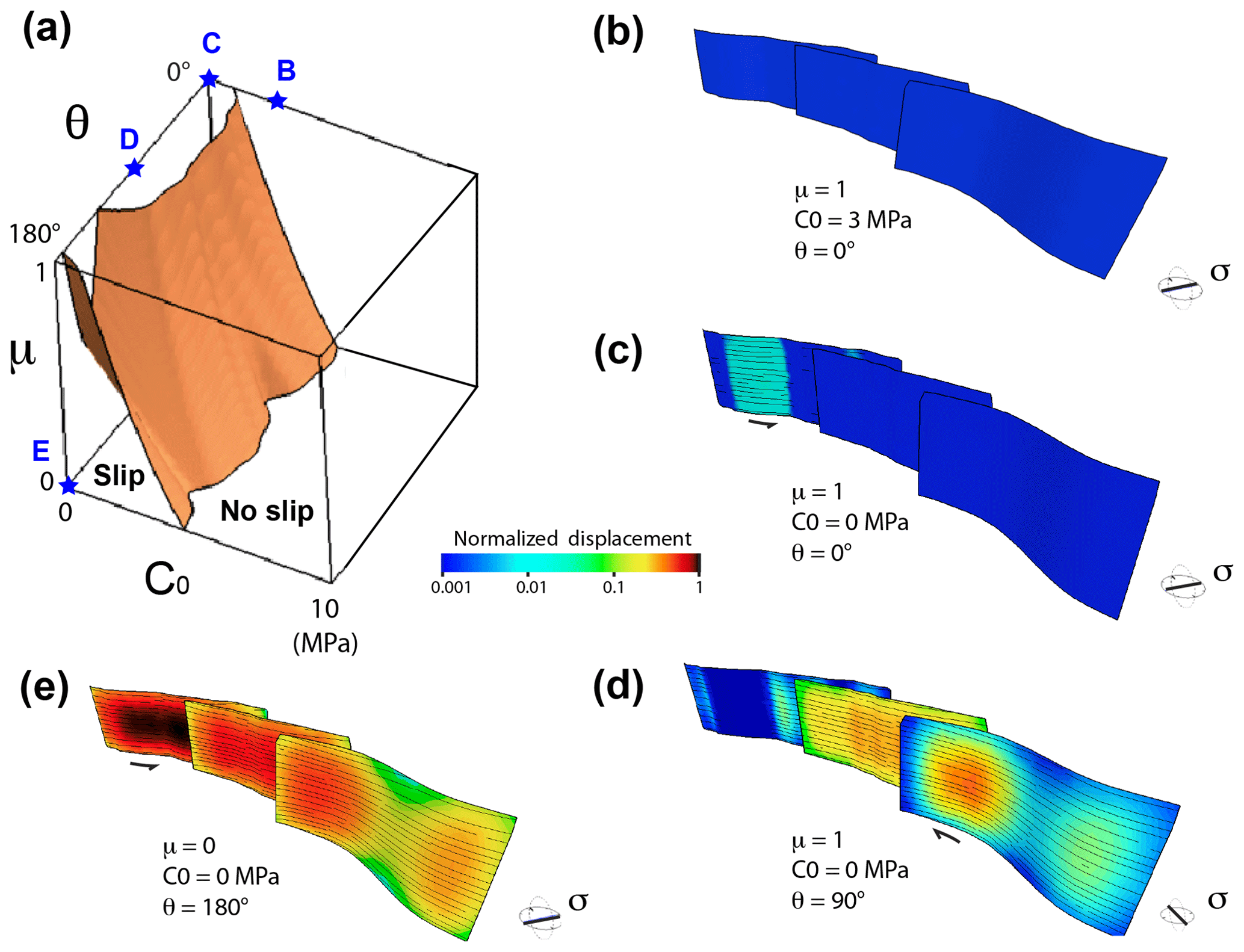
Figure 4Examples of 3-D quasi-static fault displacement distributions on the Landers model for different mechanical conditions and uniaxial stress orientation. (a) Fault slip envelope shown in Fig. 3d with reported specific model conditions used for panels (b), (c), (d), and (e) (blue stars). (b) Displacement distribution for μ=1, C0=0 MPa, and θ=0∘. (c) Displacement distribution for μ=1, C0=3 MPa, and θ=0∘. (d) Displacement distribution for μ=1, C0=0 MPa, and θ=90∘. (e) Displacement distribution for μ=0, C0=0 MPa, and θ=180∘. The color bar scale for displacement is logarithmic.
The plot of computed displacement distribution along fault is a way to analyze in which place the fault is prone to slip with respect to different parametric conditions. Some examples of computed displacement occurring on preferentially oriented parts of the fault surfaces are shown in Fig. 4 for the Landers 3-D fault geometry. Computed quasi-static fault displacement distribution is shown (blue stars) for end-member conditions of friction, cohesion, and stress orientation with respect to the position of the fault slip envelope (note that the color bar scale of displacement is logarithmic). These plots show how large values of friction coefficient allow faults to slip, revealing a very different amount and distribution of displacement as a function of θ and C0 (Fig. 4b, c, and d). Note that for θ=0 or 90∘ displacement occurs on complementary places along the faults and with opposite displacement, sinistral and dextral, respectively. The effect of mechanical interaction through the stress field (e.g. Willemse et al., 1996), although significantly lower that the role of θ, μ, or C0, is observed at fault segment overlaps. Figure 4d and e shows this effect along the displacement pattern of the first fault segment (i.e. the southern segment, see Fig. 3a), which is highly asymmetric in places where this segment has the same fault surface orientation, friction, and cohesion. Also note that stress magnitude, distribution, and orientations can be computed around fault surfaces of each “slipping” model condition. An example of stress perturbation through the stress field is shown in Fig. 5 for the conditions of θ=110∘, μ=0.4, and C0=0. Although in the range of possible friction, cohesion, and angle of σ1 with respect to the main fault trend (around 30∘), the parametric conditions shown in Fig. 5 must be considered nonrealistic since the stress loading is purely uniaxial. The absence of stress perturbation in orientation is due to this uniaxial condition and the absence of fluid pressure in this parametric study (see Kattenhorn et al., 2000, and Maerten et al., 2018). More realistic stress conditions must consider the 3-D tensor and its variation through space and time.

Figure 5Examples of quasi-static stress distribution of σ1 (a) and maximum Coulomb shear stress (b) around the Landers fault model, computed for θ=110∘, μ=0.4, and C0=0.
3.2 The Olkiluoto fault system
The 3-D shape of the fault slip envelope obtained using stress variations as proposed in Sect. 2.2 is quite simple in its geometry with a curvature in the upper corner where cohesion and ice thickness are low and friction is relatively high (Fig. 6c). This reveals that fault slip is promoted for small ice thicknesses (or vertical load) in thrust-fault regime, especially for low cohesion, allowing slip even for relatively high friction values. Other envelopes (pink) are shown in the slip domain of the diagram. These surfaces are not fault slip envelopes but envelopes of values of equal maximum quasi-static displacement computed along faults, calculated in each model. These envelopes, which depict two specific values of computed maximum displacement for different mechanical and loading conditions, mimic the shape of the fault slip envelope in the slip domain. They confirm the shape of the slip envelope and reveal that the largest ability of fault to accumulate displacement is expected for models with unrealistic conditions of no fault friction, no cohesion, and no ice sheet. Since quasi-static displacement takes into account fault interaction through the stress field, and that fault slip envelope does not, the similar shape of these three envelopes reveals the lesser influence of fault mechanical interaction compared to the effect of varying friction, cohesion, and stresses in the ranges considered in this study.
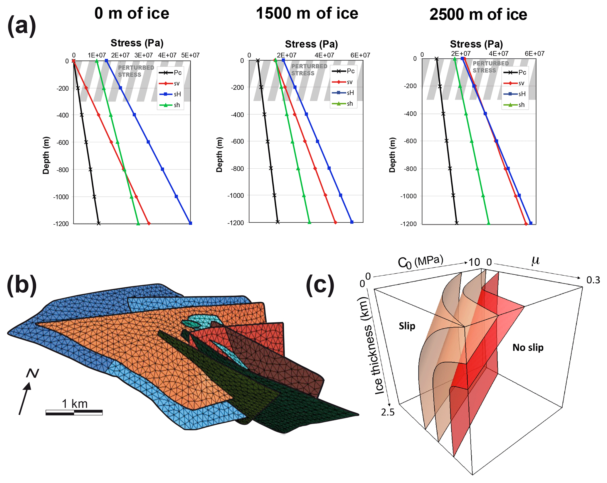
Figure 6Case study of the Olkiluoto fault system. (a) Stress state in the rock mass applied to the fault system, measured at the present day (0 m of ice) and calculated for future conditions as a function of the thickness of ice sheet cover (for 1500 and 2500 m of ice). The maximum horizontal stress (σH) is oriented E–W. (b) 3-D geometry of the fault system at the nuclear waste site. (c) Fault slip envelope of the Olkiluoto fault system (red surface) calculated using variable friction, cohesion, and stress profiles derived from 0 to 2500 m of ice sheet cover (a). The two pink surfaces are envelopes of values of equal maximum quasi-static displacement computed along faults, each one corresponding to a specific value of displacement (0.02 and 0.06 m). See the main text for further details.
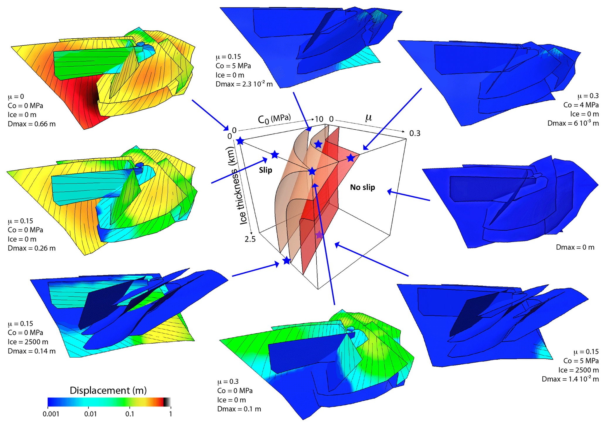
Figure 7Examples of 3-D quasi-static fault displacement distribution on the Olkiluoto model for different loading and fault property conditions indicated on the fault slip diagram by blue stars. Streamlines on fault surfaces are slickenlines. The color bar scale for displacement is logarithmic.
Quasi-static displacement distributions along fault slipping patches are shown in Fig. 7 in colored areas (the color bar scale is logarithmic) containing streamlines representing the orientation of fault slip, referred to as “slickenlines”. Displacements are computed for individual models of parametric conditions shown on the envelope with blue stars. We chose to show end-member cases, i.e. far and progressively closer to the main fault slip envelope, with roughly different parametric conditions. Displacement distribution varies from one model to another and is heterogeneous within a same model as a function of fault plane orientation, friction, and applied stress state with changing ice thickness. Consistent with the shape of the envelopes, the ability of slip to initiate and accumulate is enhanced for conditions of low friction, low cohesion, and no ice sheet cover for which most of the faults are slipping (maximum displacement lower than 0.7 m). Closer to the main fault slip envelope, slip occurs on areas restricted to the lower or upper parts of the faults, better oriented to slip (upper part), and/or for which the differential stress applied in remote conditions is the largest (lower part). Fault slip close to the Earth's surface is possible only for conditions of no ice sheet cover and moderate friction (0.15 to 0.3). Slickenlines of reverse and strike-slip movements can slightly change along a single fault surface. These changes in orientation are mainly governed by changing remote stress state with depth (Fig. 6a).
We defined fault slip envelope and therefore quantified the strength of large rock volumes containing faults as a function of friction, cohesion, and remote stresses. In the first order, our parametric study of simple to complex fault systems reveals that their strength can be assessed as a function of their degree of geometric complexity. The more complex is the geometry, the simpler the fault slip envelopes. Complex fault systems always have optimally oriented fault surfaces that can slip with respect to the boundary stress conditions applied. In contrast, fault systems having limited fault orientations relative to the principal remote stresses provide strong strength anisotropy such as revealed by strong curvature of the fault slip envelope in the direction of θ. Also worth noting is that the strength anisotropy varies with the values of friction of the fault surfaces. This general behavior is inherent to the Mohr–Coulomb frictional-slip theory, for which fault slip with respect to the stress orientation and state depends on the friction coefficient (Hatheway and Kiersch, 1989; Scholz, 2019).
The case study of the Olkiluoto nuclear waste repository site allowed us to apply this technique on a fault system subjected to realistic stress loading conditions. The resulting fault slip envelope for the Olkiluoto system shows the importance of the 3-D geometry of the fault system, but also the critical importance of the applied geological stresses. For the present-day context of no ice sheet (interglacial period), this fault system is subjected to a thrust-fault stress regime governed by the E–W push from the Mid-Atlantic Ridge. This geological context seems to provide the best conditions for fault slip because of the highest resolved shear stress on low dipping fault surfaces. Such fault surfaces are optimally oriented to slip under a thrust-fault stress regime with S1 oriented E–W and with large values of differential stress applied, especially close to the Earth's surface for these conditions of no ice thickness (Fig. 6a, 0 m of ice). Even for high friction values, optimally oriented fault surfaces could therefore be critically stressed in the present day.
Although the actual conditions provide the largest resolved shear stress on fault plane, the main results obtained are in agreement with the actual conditions observed at the Olkiluoto repository site, where no slip is monitored or observed along faults under the actual conditions. Although probably variable along fault surfaces, the fault rock mechanical properties derived from mechanical tests suggest a static friction and cohesion larger than the conditions computed to allow fault slip. The worst case scenario would corresponds to the upper-right 3-D model result shown in Fig. 7 (μ=0.3, C0=4 MPa, no ice thickness) where fault slip might occur in a very limited upper part of the fault model. Also note that the actual stress profiles (referred to as “no ice thickness”, Fig. 6a, 0 m of ice) are not well defined close to the Earth's surface and probably overestimated because of the loss of rock cohesion due to the presence of open fracture patterns and rock alteration (Ask, 2011; Hudson et al., 2008; Mönkkönen et al., 2012).
The increase in thickness of an ice sheet implies progressive stress permutation to the strike-slip regime in the stress profiles (Fig. 6a). The general low dip of the faults (non-optimal orientation) combined with a low differential stress, inherent to this strike-slip regime, provide conditions for low resolved shear stresses on faults, and therefore better general strength of the fault system (also see Johnston, 1987). The planar and vertical shape of the fault slip envelope in this lower part of the diagram reveals the little dependence of fault strength on the vertical load increase, here the value of S2 (or the Lode angle). Given the range of friction and cohesion estimated using mechanical tests, such conditions of increasing ice thickness must be unfavorable for fault slip. However, as mentioned in Sect. 2.2, such a range might strongly evolve through time and space, outside of the sampled areas, due to the presence of fluids or variations of fault rock properties.
A potential limitation of the proposed technique relies on the uncertainty and biases of the 3-D fault surface discretization. In the example of Olkiluoto, uncertainties in fault surface geometry were estimated from a significant amount of data available from bore hole, seismic profiles, tunnel wall observations, and outcrop measurements (Mattila et al., 2008). Truncation bias is here defined by not considering the faults smaller than 100 m length estimated to allow incremental displacement lower than 10−2 m (Wells and Coppersmith, 1994). Variability or uncertainty in in situ stresses and rock material properties estimated from bore hole and rock tests are not considered limitations since they are used to constrain their range of variability in the parametric study (see Sect. 2.2). This approach is actually particularly suitable to address uncertainties in input data and any hazard assessment. On the other hand, oversight or mistakes in the choice of the variables considered in the model can be a major limitation in the approach. In the Olkiluoto example we chose to consider friction, cohesion, and especially the stress state as the main variables, rather than, for example, the role of water pressure. Although variation in hydraulic head in the vadose/aquifer zone considered is expected during the glacial period (Lemieux et al., 2008), it has no effect on anisotropy of strength since water pressure is isotropic, and thus does not change the shape of the fault slip envelope. Furthermore, expected water pressures are 1 order of magnitude lower (several MPa) than tectonic stresses (20 to 60 MPa), and would very slightly displace the fault slip envelope toward the right-hand side of the diagrams shown in Figs. 6c and 7. The effect of water on static friction weakening of the altered fault rocks is probably much more important (more than 50 % reduction of friction in clays; Morrow et al., 2000), and is indirectly considered in the range of friction used in the parametric study (). A last limitation concerns the quasi-static elastic fault displacement patterns computed in places where slip occurs (Fig. 5). As mentioned in the method section, this displacement distribution must be seen as a fault's ability to initiate and accumulate slip. Even though quasi-static models generally provide good results (e.g. Pollard and Fletcher, 2005; p. 308, chapter 8.3.3 and Fig. 8.15), realistic coseismic displacement distribution and subsequent stress perturbation in the surroundings can be better approached using dynamic rupture propagation processes and dynamic friction laws in softening or hardening fault rocks as a function of material properties and new stress field around the first slipping fault in the model.
A new tool referred to as “fault slip envelope” is proposed in order to provide complementary analysis to the conventional methods used for fault slip or slip tendency:
-
Fault slip is calculated along simple or very complex fault geometry on DFN using the resolved shear and normal stresses with respect to the Mohr–Coulomb frictional slip theory and quasi-static elastic behavior. This method allows for considering friction and cohesion as potential variables through space and time.
-
Combining a 3-D boundary element model and fast computation method allows the user to run thousands of forward simulations in a very short time, and therefore to provide a full parametric study with a wide range of variable mechanical conditions such as stress orientation and magnitude.
-
This technique allows the user, for the first time, to propose “fault slip envelopes” which quantify fault system strength magnitude and anisotropy as a function of important parameters, which are either unknown and/or considered variable through time and space. This can be useful to address uncertainties in input data for hazard assessment.
-
We also calculate fault displacement based on a quasi-static elastic solution allowing mechanical interaction through the stress field in places where the Coulomb's criterion is reached along each fault of a DFN.
The quantification of the strength of fault systems in 3-D underlines the importance of accuracy in deterministic studies of geological structures and stresses. Beyond its societal application to fault slip hazard, geological storage, geothermal systems, and reservoir leaks, this technology also provides new considerations and perspectives in the analysis of fault systems and Earth's crust strength. Major earthquakes at plate boundaries occur on relatively simple fault systems, such as large strike-slip faults or subduction plate megathrusts (Berryman et al., 2012; Chester et al., 2013; also see Fig. 3a), where the strength is definitely anisotropic and thoroughly depends on stress orientation and fault zone properties (e.g. Fig. 3d). It is nevertheless also well known that large earthquakes can occur on more complex fault geometries, as for example in the Kaikoura and Darfield fault systems in New Zealand's South Island (Beavan et al., 2012; Hamling et al., 2017; Ulrich et al., 2019) or in the Sierra Madre–Cucamonga thrust fault system in southern California (Anderson et al., 2003). In such a case, fault system strength is probably more isotropic and fault slip depends more on static friction along faults than on stress orientation (e.g. Fig. 3f). This difference in domain of stability allows for quantifying the bulk strength of the brittle crust, which is lower for complex fault geometry rather than a simple one for equivalent frictional and remote stress conditions, as recently observed in experimental modeling of a complex versus simple subduction interface (Van Rijsingen et al., 2019). As much as frictional properties or pore pressure, the degree of complexity of a fault system constitutes the basic premise for easier crustal stress relaxation and prevention of major slip events. Consequently, the precise definition and quantification of the strength in the brittle crust relies on the precise knowledge of 3-D fault geometry, constitution, and stresses at each study site. Significant progress in this field poses a challenge for future geosciences.
Data and scientific reports from the Olkiluoto nuclear site are archived and available online at the following URL: http://www.posiva.fi/en/databank\#.VukXRGdPo_w, last access: 12 July 2019.
RS conceptualized the fault slip envelopes, ran models, analysed the results, wrote the article, and did the revisions. FM wrote the numerical codes, ran models, and participated in the analysis of the results and article writing. LM ran some early models, provided 3-D fault system data, and participated in the analysis of the results. JM provided data from the Olkiluoto nuclear repository site and participated in the article writings.
A first version of this article was rejected from the journal Geology, mainly because of an existing conflict of interest with the slip tendency analysis tool. An anonymous reviewer did not see a clear scientific advance for the tool proposed here compared to the existing slip tendency method. This is why we point out in this version of the article (introduction and conclusion) the clear differences and new insights.
The authors wish to thank the associate editor Cristiano Colettini and the two anonymous reviewers for their constructive comments, which helped improve the quality of the article.
This work was initiated during a research program funded by POSIVA and IGEOSS companies, and pursued with the financial support of Geoscience Montpellier and Schlumberger.
This paper was edited by Cristiano Collettini and reviewed by two anonymous referees.
Aaltonen, I., Lahti, M., Engström, J., Mattila, J., Paananen, M., Paulamäki, S., Gehör, S, Kärki, A., Ahokas, T., Torvela, T., and Front, K.: Geological Model of the Olkiluoto Site version 2, Posiva Working Report 70, available at: http://www.posiva.fi/files/1439/WR_2010-70_web.pdf (last access: 12 July 2019), 2010.
Alvarez del Castillo, A., Alaniz-Alvarez, A. A., Nieto-Samaniego, A. F., Xu, S., Ochoa-Gonzales, G. H., and Velasquillo-Martinez, L. G.: Software for determining the direction of movement, shear and normal stresses of a fault under a determined stress state, Comput. Geosci., 104, 84–92, https://doi.org/10.1016/j.cageo.2017.03.006, 2017
Anderson, G., Aagaard, B., and Hudnut, K.: Fault Interactions and Large Complex Earthquakes in the Los Angeles Area, Science 302, 1946, https://doi.org/10.1126/science.1090747, 2003.
Arthaud, F.: Méthode de détermination graphique des directions de raccourcissement, d'allongement et intermédiaire d'une population de failles, B. Soc. Geol. Fr., 7, 729–737, 1969.
Arvidsson, R.: Fennoscandian earthquakes: Whole crust rupturing related to postglacial rebound, Science, 274, 744–746, 1996.
Ask, D.: Semi-Integration of Overcoring Stress Data and Review of Rock Stress Data at the Olkiluoto Site, Posiva Working Report 16, available at: http://www.posiva.fi/files/1705/WR_2011-16web.pdf (last access: 12 July 2019), 2011.
Beavan, J., Motagh, M., Fielding, E. J., Donnelly, N., and Collett, D.: Fault slip models of the 2010–2011 Canterbury, New Zealand, earthquakes from geodetic data and observations of postseismic ground deformation, N. Z. J. Geol. Geophys., 55, 207–221, https://doi.org/10.1080/00288306.2012.697472, 2012.
Berger, A. and Loutre, M. F.: Paleoclimate sensitivity to CO2 and insolation, Ambio, 26, 32–37, 1997.
Berryman, K. R., Cochran, U. A., Clark, K. J., Biasi, G. P., Langridge, R. M., and Villamor, P.: Major Earthquakes Occur Regularly on an Isolated Plate Boundary Fault, Science, 336, 1690–1693, https://doi.org/10.1126/science.1218959, 2012.
Brantut, N., Heap, M. J., Meredith, P. G., and Baud, P.: Time-dependent cracking and brittle creep in crustal rocks: A review, J. Struct. Geol., 52, 17–43, https://doi.org/10.1016/j.jsg.2013.03.007, 2013.
Byerlee, J. D.: Friction of rocks, Pure Appl. Geophys., 116, 615–626, 1978.
Chester, F. M., Rowe, C., Ujiie, K., Kirkpatrick, J., Regalla, C., Remitti, F., Moore, J. C., Toy, V., Wolfson-Schwehr, M., Bose, S., Kameda, J., Mori, J. J., Brodsky, E. E., Eguchi, N., and Toczko, S.: Structure and Composition of the Plate-Boundary Slip Zone for the 2011 Tohoku-Oki Earthquake, Science, 342, 1208, https://doi.org/10.1126/science.1243719, 2013.
Collettini, C. and Trippetta, F.: A slip tendency analysis to test mechanical and structural control on aftershock rupture planes, Earth Planet. Sci. Lett., 255, 402–413, 2007.
Collettini, C., Niemeijer, A., Viti, C., and Marone, C.: Fault zone fabric and fault weakness, Nature, 462, 907–911, 2009.
Crider, J. G. and Pollard, D. D.: Fault linkage: Three-dimensional mechanical interaction between echelon normal faults, J. Geophys. Res.-Sol. Ea., 103, 24373–24391, https://doi.org/10.1029/98JB01353, 1998.
Faulkner, D. R., Mitchell, T. M., Healy, D., and Heap, M. J.: Slip on “weak” faults by the rotation of regional stress in the fracture damage zone, Nature, 444, 922–925, 2006.
Forsyth, D. and Uyedaf, S.: On the Relative Importance of the Driving Forces of Plate Motion, Geophys. J. Roy. Astronom. Soc., 43, 163–200, https://doi.org/10.1111/j.1365-246X.1975.tb00631.x, 1975.
Grollimund, B. and Zoback, M. D.: Post glacial lithospheric fexure and induced stresses and pore pressure changes in the northern North Sea, Tectonophysics, 21, 61–81, 2000.
Hackston, A. and Rutter, E.: The Mohr–Coulomb criterion for intact rock strength and friction – a re-evaluation and consideration of failure under polyaxial stresses, Solid Earth, 7, 493–508, https://doi.org/10.5194/se-7-493-2016, 2016.
Hakkala, M., Siren, T., Kemppainen, K., Christiansson, R., and Martin, D.: In Situ Stress Measurement with the New LVDT-cell – Method Description and Verification, Posiva Working Report 2012-43, available at: http://www.posiva.fi/files/3448/POSIVA_2012-43.1.pdf (last access: 12 July 2019), 2013.
Hamling, I. J., Hreinsdóttir, S., Clark, K., Elliott, J., Liang, C., Fielding, E., Litchfield, N., Villamor, P., Wallace, L., Wright, T. J., D'Anastasio, E., Bannister, S., Burbidge, D., Denys, P., Gentle, P., Howarth, J., Mueller, C., Palmer, N., Pearson, C., Power, W., Barnes, P., Barrell, D. J. A., Van Dissen, R., Langridge, R., Little, T., Nicol, A., Pettinga, J., Rowland, J., and Stirling, M.: Complex multifault rupture during the 2016 Mw 7.8 Kaikōura earthquake, New Zealand, Science, 356, eaam7194, https://doi.org/10.1126/science.aam7194, 2017.
Hatheway, A. W. and Kiersch, G. A. (Eds.): Engineering properties of rock, R.S. Carmichael, Practical Handbook of Physical Properties of Rocks and Minerals, CRC Press, Boca Raton, 672–715, 1989.
Healy, D., Blenkinsop, T. G., Timms, N. E., Meredith, P. G., Mitchell, T. M., and Cooke, M. L.: Polymodal faulting: Time for a new angle on shear failure, J. Struct. Geol., 80, 57–71, https://doi.org/10.1016/j.jsg.2015.08.013, 2015.
Holdsworth, R. E.: Weak Faults–Rotten Cores, Science, 303, 181, https://doi.org/10.1126/science.1092491, 2004.
Hudson, J. A., Cosgrove, J. W., and Johansson, E.: Estimating the Mechanical Properties of the Brittle Deformation Zones at Olkiluoto, Posiva Working Report 67, available at: http://www.posiva.fi/files/800/WR2008-67web.pdf (last access: 12 July 2019), 2008.
Jaeger, J. C. and Cook, N. G. W. (Eds.): Fundamentals of Rock Mechanics, Chapman and Hall, New York, 1979.
Johnston, A. C.: Suppression of earthquakes by large continental ice sheets, Nature, 330, 467–469, https://doi.org/10.1038/330467a0, 1987.
Karlstrom, K. E. and Williams, M. L.: Heterogeneity of the middle crust: Implications for strength of continental lithosphere, Geology, 26, 815–818, https://doi.org/10.1130/0091-7613(1998)026<0815:HOTMCI>2.3.CO;2, 1998.
Kattenhorn, S. A. and Pollard, D. D.: Integrating 3D seismic data, field analogs and mechanical models in the analysis of segmented normal faults in the Wytch Farm oil field, southern England, AAPG Bull., 85, 1183–1210, 2001.
Kattenhorn, S. A., Aydin, A., and Pollard, D. D.: Joints at high angles to normal fault strike: an explanation using 3-D numerical models of fault-perturbed stress field, J. Struct. Geol., 23, 1–23, 2000.
Lejri, M., Maerten, F., Maerten, L., and Soliva, R.: Accuracy evaluation of both Wallace-Bott and BEM-based paleostress inversion methods, Tectonophysics, 694, 130–145, https://doi.org/10.1016/j.tecto.2016.11.039, 2017.
Lemieux, J.-M., Sudicky, E. A., Peltier, W. R., and Tarasov, L.: Dynamics of groundwater recharge and seepage over the Canadian landscape during the Wisconsinian glaciation, J. Geophys. Res.-Earth Surf., 113, F01011, https://doi.org/10.1029/2007JF000838, 2008.
Lisle, R. J. and Srivastava, D. C.: Test of the frictional reactivation theory for faults and validity of fault-slip analysis, Geology, 32, 569–572, https://doi.org/10.1130/G20408.1, 2004.
Lovely, P. J., Pollard, D. D., and Mutlu, O.: Regions of Reduced Static Stress Drop near Fault Tips for Large Strike-Slip EarthquakesRegions of Reduced Static Stress Drop near Fault Tips for Large Strike-Slip Earthquakes, B. Seismol. Soc. Am., 99, 1691–1704, https://doi.org/10.1785/0120080358, 2009.
Madden, E. H., Maerten, F., and Pollard, D. D.: Mechanics of nonplanar faults at extensional steps with application to the 1992 M 7.3 Landers, California, earthquake: J. Geophys. Res.-Sol. Ea., 118, 3249–3263, https://doi.org/10.1002/jgrb.50237, 2013.
Maerten, F., Maerten, L., and Cooke, M.: Solving 3D boundary element problems using constrained iterative approach, Comput. Geosci., 14, 551–564, https://doi.org/10.1007/s10596-009-9170-x, 2010.
Maerten, F., Maerten, L., and Pollard, D. D.: iBem3D, a three-dimensional iterative boundary element method using angular dislocations for modeling geologic structures, Comput. Geosci., 72, 1–17, https://doi.org/10.1016/j.cageo.2014.06.007, 2014.
Maerten, L., Pollard, D. D., and Maerten, F.: Digital mapping of three-dimensional structures of the Chimney Rock fault system, central Utah, J. Struct. Geol., 23, 585–592, https://doi.org/10.1016/S0191-8141(00)00142-5, 2001.
Maerten, L., Gillespie, P., and Pollard, D. D.: Effects of local stress perturbation on secondary fault development, J. Struct. Geol., 24, 145–153, https://doi.org/10.1016/S0191-8141(01)00054-2, 2002.
Maerten, L., Maerten, F., and Lejri, M.: Along fault friction and fluid pressure effects on the spatial distribution of fault-related fractures, J. Struct. Geol., 108, 198–212, https://doi.org/10.1016/j.jsg.2017.10.008, 2018.
Marrett, R. and Allmendinger, R. W.: Kinematic analysis of fault-slip data, J. Struct. Geol., 12, 973–986, https://doi.org/10.1016/0191-8141(90)90093-E, 1990.
Mattila, J. and Viola, G.: New constraints on 1.7 Gyr of brittle tectonic evolution in southwestern Finland derived from a structural study at the site of a potential nuclear waste repository (Olkiluoto Island), J. Struct. Geol., 67, 50–74, https://doi.org/10.1016/j.jsg.2014.07.003, 2014.
Mattila, J., AAltonen, I., Kemppainen, I., Wikström, L., Paananen, M., Paulamäki, S., Front, K., Gehör, S., Kärki, A., and Ahokas, T.: Geological Model of the Olikiluotto Site, Version 1.0, Olkiluoto, Posiva Working Report 2007-92, available at: https://inis.iaea.org/collection/NCLCollectionStore/_Public/43/063/43063338.pdf?r=1&r=1 (last access: 12 July 2019), 2008.
McLaskey, G. C., Thomas, A. M., Glaser, S. D., and Nadeau, R. M.: Fault healing promotes high-frequency earthquakes in laboratory experiments and on natural faults, Nature, 491, 101–105, 2012.
Moeck, I., Kwiatek, G., and Zimmermann, G.: Slip tendency analysis, fault reactivation potential and induced seismicity in a deep geothermal reservoir, J. Struct. Geol., 31, 1174–1182, https://doi.org/10.1016/j.jsg.2009.06.012, 2009.
Mönkkönen, H., Hakkala, M., Paananen, M., and Laine, E.: Onkalo Rock Mechanics Model Version 2, Posiva Working Report 07, available at: http://www.posiva.fi/files/2026/WR_2012-07web.pdf (last access: 12 July 2019), 2012.
Morris, A., Henderson, D. B., and Ferrill, D. A.: Slip-tendency analysis and fault reactivation, Geology, 24, 275–278, https://doi.org/10.1130/0091-7613(1996)024<0275:STAAFR>2.3.CO;2, 1996.
Morrow, C. A., Moore, D. E., and Lockner, D. A.: The effect of mineral bond strength and adsorbed water on fault gouge frictional strength, Geophys. Res. Lett., 27, 815–818, https://doi.org/10.1029/1999GL008401, 2000.
Neves, M. C., Paiva, L. T., and Luis, J.: Software for slip-tendency analysis in 3D: A plug-in for Coulomb, Comput. Geosci., 35, 2345–2352, https://doi.org/10.1016/j.cageo.2009.03.008, 2009.
Nicol, A., Watterson, J., Walsh, J. J., and Childs, C.: The shapes, major axis orientations and displacement patterns of fault surfaces, J. Struct. Geol., 18, 235–248, https://doi.org/10.1016/S0191-8141(96)80047-2, 1996.
Olson, J. E. and Pollard, D. D.: The initiation and growth of en echelon veins, J. Stuct. Geol., 13, 595–608, 1991.
Pollard, D. D. and Fletcher, R. C. (Eds.): Fundamentals of Structural Geology, Cambridge University Press, London, 2005.
Reches, Z. and Dieterich, J. H.: Faulting of rocks in threedimensional strain fields, I. failure of rocks in polyaxial, servocontrol experiments, Tectonophysics, 95, 111–132, 1983.
Rutter, E. H. and Glover, C. T.: The deformation of porous sandstones; are Byerlee friction and the critical state line equivalent?, J. Struct. Geol., 44, 129–140, https://doi.org/10.1016/j.jsg.2012.08.014, 2012.
Scholz, C. H.: The Mechanics of Earthquakes and Faulting, 3rd edn., Cambridge University Press, Cambridge, 2019.
Sjöberg, J.: Overcoring Rock Stress Measurements in Borehole OL-KR24, Olkiluoto, Posiva Working Report 60, available at: http://www.posiva.fi/files/2238/POSIVA-2003-60_Working-report_web.pdf (last access: 12 July 2019), 2003.
Skinner, B. J. and Porter, S. C. (Eds.): Physical Geology, John Wiley & Sons, New York, 1987.
Soliva, R., Benedicto, A., Schultz, R. A., Maerten, L., and Micarelli, L.: Displacement and interaction of normal fault segments branched at depth: Implications for fault growth and potential earthquake rupture size, J. Struct. Geol., 30, 1288–1299, https://doi.org/10.1016/j.jsg.2008.07.005, 2008.
Thomas, A. L.: Poly3D: a three-dimensional, polygonal element, displacement discontinuity boundary element computer program with applications to fractures, faults, and cavities in the earth's crust, MS thesis, Stanford University, Stanford, California, USA, 1993.
Townend, J. and Zoback, M. D.: How faulting keeps the crust strong, Geology, 28, 399–402, https://doi.org/10.1130/0091-7613(2000)28<399:HFKTCS>2.0.CO;2, 2000.
Ulrich, T., Gabriel, A.-A., Ampuero, J.-P., and Xu, W.: Dynamic viability of the 2016 Mw 7.8 Kaikōura earthquake cascade on weak crustal faults, Nat. Commun., 10, https://doi.org/10.1038/s41467-019-09125-w, 2019.
Van Rijsingen, E., Funiciello, F., Corbi, F., and Lallemand, S.: Rough Subducting Seafloor Reduces Interseismic Coupling and Mega-Earthquake Occurrence: Insights From Analogue Models, Geophys. Res. Lett., 46, 3124–3132, https://doi.org/10.1029/2018GL081272, 2019.
Wells, D. L. and Coppersmith, K. J.: New empirical relationships among magnitude, rupture length, rupture width, rupture area, and surface displacement, B. Seismol. Soc. Am., 84, 974–1002, 1994.
Wibberley, C. A. J., Yielding, G., and Di Toro, G.: Recent advances in the understanding of fault zone internal structure: a review, Geol. Soc. Lond. Spec. Pub., 299, 5, https://doi.org/10.1144/SP299.2, 2008.
Willemse, E. J. M., Pollard, D. D., and Aydin, A.: Three-dimensional analyses of slip distributions on normal fault arrays with consequences for fault scaling, J. Struct. Geol., 18, 295–309, https://doi.org/10.1016/S0191-8141(96)80051-4, 1996.
Yukutake, Y., Takeda, T., and Yoshida, A.: The applicability of frictional reactivation theory to active faults in Japan based on slip tendency analysis, Earth Planet. Sci. Lett., 411, 188–198, https://doi.org/10.1016/j.epsl.2014.12.005, 2015.