Stress characterization and temporal evolution of borehole failure at the Rittershoffen geothermal project

In the Upper Rhine Graben, several innovative projects based on enhanced geothermal system (EGS) technology exploit local deep-fractured geothermal reservoirs. The principle underlying this technology consists of increasing the hydraulic performances of the natural fractures using different stimulation methods in order to circulate the natural brine at commercial flow rates. For this purpose, knowledge of the in situ stress state is of central importance to predict the response of the rock mass to different stimulation programs. Here, we propose a characterization of the in situ stress state from the analysis of ultrasonic borehole imager (UBI) data acquired at different key moments of the reservoir development using a specific image correlation technique. This unique dataset has been obtained from the open-hole sections of the two deep wells (GRT-1 and GRT-2, ∼2500 m) at the geothermal site of Rittershoffen, France. We based our analysis on the geometry of breakouts and drilling-induced tension fractures (DITFs). A transitional stress regime between strike-slip and normal faulting consistent with the neighboring site of Soultz-sous-Forêts is evident. The time-lapse dataset enables us to analyze both in time and space the evolution of the structures over 2 years after drilling. The image correlation approach developed for time-lapse UBI images shows that breakouts extend along the borehole with time and widen (i.e., angular opening between the edges of the breakouts) but do not deepen (i.e., increase in the maximal radius of the breakouts). The breakout widening is explained by wellbore thermal equilibration. A significant stress rotation at depth is evident. It is shown to be controlled by a major fault zone and not by the sediment–basement interface. Our analysis does not reveal any significant change in the stress magnitude in the reservoir.

1 Introduction

Several deep geothermal projects located in the Upper Rhine Graben based on enhanced geothermal system (EGS) technology exploit local geothermal reservoirs, such as those located in Soultz-sous-Forêts and in Rittershoffen (Baujard et al., 2017; Genter et al., 2010). The principle underlying this technology consists of increasing the hydraulic performance of the reservoir through different types of simulations to achieve commercially interesting flow rates. The stimulation techniques are typically based on high-pressure injection (hydraulic stimulation), cold water injection (thermal stimulation) or chemical injection (chemical stimulation). During the injections, a thermo-hydro-chemo-mechanical perturbation induces an increase in permeability due to the reactivation of existing structures or the generation of new ones (Cornet, 2015; Huenges and Ledru, 2011). The in situ stress state is a key parameter controlling rock mass response during stimulation and is required to design stimulation strategies and forecast the response of the reservoir to varying injection schemes.

Despite its importance, the in situ stress state is difficult to assess, particularly in situations in which the rock mass is only accessible through a few deep boreholes. In such cases, the assessment of borehole walls using borehole logging imaging is a useful technique to provide information on the type, the orientation and the size of fractures or breakouts, which are due to stress perturbations related to the existence of the well (drilling and fluid boundary conditions). Subsequently, it gives useful constraints on the in situ stress state surrounding the wellbore (Schmitt et al., 2012; Zoback et al., 2003). Borehole breakouts provide indirect information on the stress orientation that it is difficult to extract, in particular for robust quantitative stress magnitudes. Indeed, it relies on the choice of the failure model used to interpret borehole wall images. The mechanisms that control the failure evolution of the borehole wall are not well understood in space or time, and there is no consensus on the most appropriate failure criteria to be used. Parameterizing failure criteria is also a challenge since intact core material is often not available from deep boreholes. Finally, the set of images used to identify borehole failures is typically acquired a few days after drilling completion when it is unclear if the geometry has reached a new stationary state. The present analysis addresses these difficulties as we attempt to characterize the stress state at the Rittershoffen geothermal site (France).

We first present in this paper the geological and geodynamical context of the Rittershoffen geothermal site (France). We describe the borehole imaging data acquired in the GRT-1 and GRT-2 wells at the Rittershoffen geothermal project. We then proceed to a brief review of the methods used for ultrasonic borehole imager (UBI) analyses with their underlying assumptions. We applied the methodology proposed by Schmitt et al. (2012) and Zoback et al. (2003) in order to assess the stress state at this site. To analyze the three successive images of the wellbore acquired up to 2 years after drilling completion, we developed an image processing method for the UBI data to compare in time the geometry of breakouts. We deduce from this study the evolution of breakouts with time and evaluate its impact on our in situ stress state assessment. We finally propose our best estimate of the in situ stress state for the Rittershoffen site, both in orientation and magnitude.

2 Rittershoffen project context

The Rittershoffen geothermal project, also referred to as the ECOGI project, is located near the village of Rittershoffen in northeastern France (Alsace). It is an EGS geothermal project initiated in 2011 (Baujard et al., 2015, 2017). The doublet has been drilled between Rittershoffen and Betschdorf, 6 km east of the Soultz-sous-Forêts geothermal project in northern Alsace, France (Genter et al., 2010). The aim of the project is to deliver heat through a long pipeline loop to the Roquette Frères bio-refinery located 15 km away. The power plant capacity is 24 MWth, intending to cover up to 25 % of the client heat need. Figure 1 gives an overview of the project location and presents in the right insert the trajectory and completion of the wells, GRT-1 and GRT-2, that have been drilled (Baujard et al., 2017). GRT-1 was completed in December 2013. It was drilled to a depth of 2580 m (MD, depth measured along hole), corresponding to a vertical depth (TVD) of 2562 m. The well penetrates the crystalline basement at a depth of 2212 m MD and targets a local complex fault structure (Baujard et al., 2017; Lengliné et al., 2017; Vidal et al., 2016). The 8^′′ 1∕2 diameter open-hole section of the well starts at 1922 m MD. The borehole is almost vertical with a maximum deviation of 9^∘ only. The first hydraulic tests concluded with an insufficient injectivity of the injection well GRT-1. Therefore, the well was stimulated in 2013, which resulted in a fivefold increase in the injectivity (Baujard et al., 2017). The target of the production well GRT-2 and its trajectory have been designed to benefit from the results of additional seismic profiles acquired in the meantime. GRT-2 targets the same fault structure but more than 1 km away from GRT-1. Local complexities of the fault structure such as “in-step” geometry have been observed a posteriori from micro-seismic monitoring during GRT-1 stimulation (Lengliné et al., 2017). The GRT-2 borehole was drilled in 2014 to a total depth of 3196 m MD (2708 m TVD) (Baujard et al., 2017). The granite basement is penetrated at a depth of 2493.5 m MD. The 8^′′ 1∕2 diameter open-hole section starts at a depth of 2120 m MD. This borehole is directed to the north and is strongly deviated with a mean deviation of 37^∘ over the interval of interest. The left insert of Fig. 1 shows more specifically the geological units penetrated by the deep boreholes of the geothermal sites in Rittershoffen and Soultz-sous-Forêts. It consists of sedimentary layers from the Cenozoic and Mesozoic that are overlaying a crystalline basement made of altered and fractured granitic rocks (Aichholzer et al., 2016). Natural fractures are well developed in the Vosges sandstones and Annweiler sandstones, as in the granitic basement. The fracture network was observed from acoustic wall imagery in the open-hole sections of GRT-1 and GRT-2 and analyzed by Vidal (2017). The analysis of the major continuous natural fractures concluded, in GRT-1, with a global orientation of N 15^∘ E to N 20^∘ E with a dip of 80^∘ W. In GRT-2, the main fracture family is oriented N 155^∘ E to N 175^∘ E with a dip of 80^∘ E to 90^∘ E. Fracture density is the highest on the roof of the granitic basement (Vidal, 2017). Oil and gas exploration in the area led to good knowledge of the regional subsurface, including measures of temperatures at depth. The unusually high geothermal gradient encountered in Soultz-sous-Forêts, which is one of the largest described so far in the Upper Rhine Graben, encouraged the development of the ECOGI project in this area (Baujard et al., 2017).

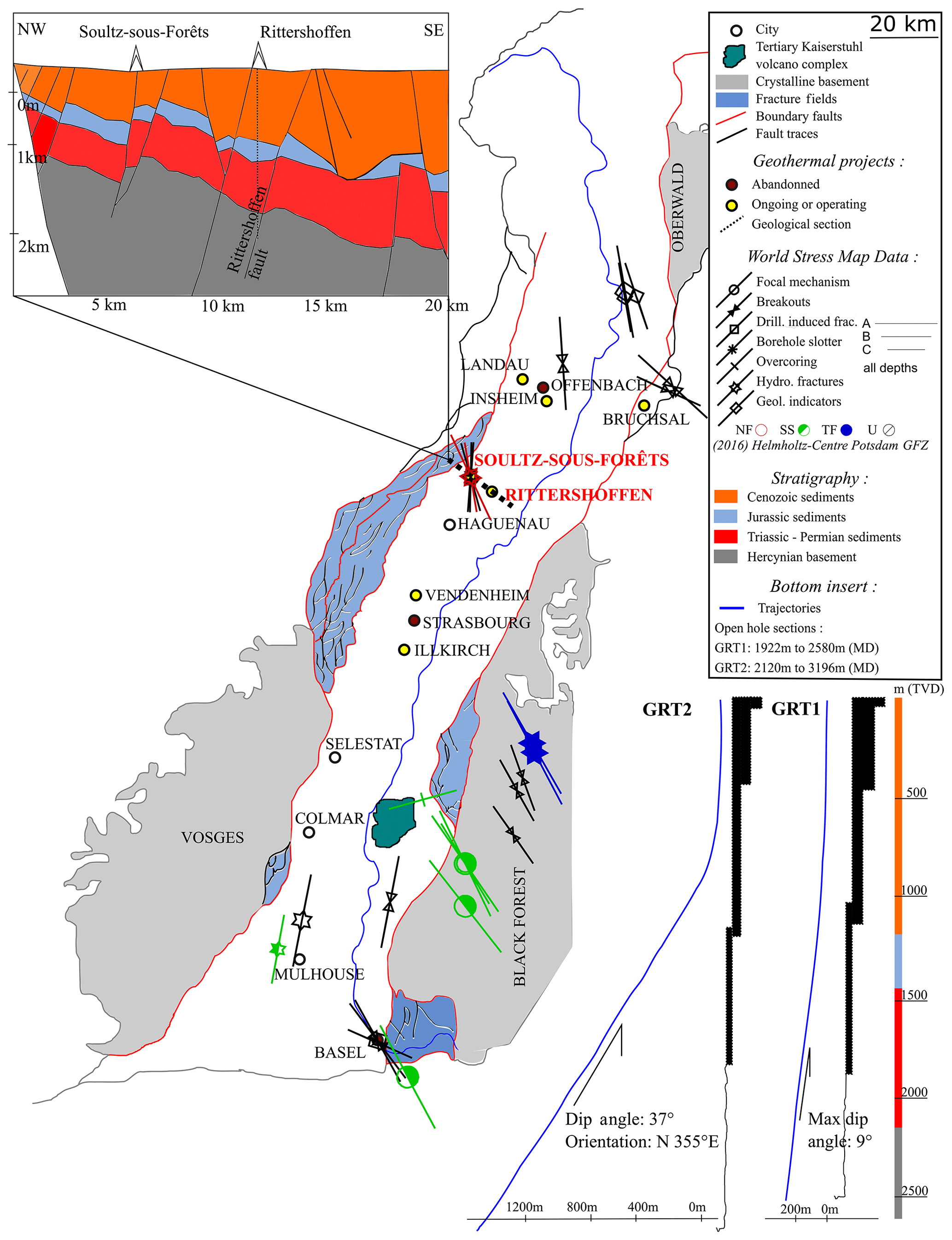
Figure 1 Geological and structural map of the main Upper Rhine Graben with the location of the Rittershoffen and Soultz-sous-Forêts sites. The map also shows the location and status of other neighboring deep geothermal projects. It includes stress data from the World Stress Map database (Heidbach et al., 2016). The upper left insert shows a geological section highlighting the main units crossed by the wells in Rittershoffen and Soultz-sous-Forêts (Aichholzer et al., 2016; Baujard et al., 2017). The lower right insert is a sketch of wells GRT-1 and GRT-2 drilled in Rittershoffen, which includes their geometry, depths and crossed lithology (after Baujard et al., 2015, 2017).

The geological context is characterized in the vicinity of the Soultz-sous-Forêts and Rittershoffen sites from numerous studies owing to extended geophysical exploration in the region (Aichholzer et al., 2016; Cornet et al., 2007; Dezayes et al., 2005; Dorbath et al., 2010; Evans et al., 2009; Genter et al., 2010; Rummel, 1991; Rummel and Baumgartner, 1991). Given that the GRT-1 and GRT-2 wells penetrate geologic units similar to those in Soultz-sous-Forêts, information from the Soultz-sous-Forêts site can be used to better characterize the geological units through which the wells in Rittershoffen are drilled (Aichholzer et al., 2016; Vidal et al., 2016). It can be used, in particular, for the strength and mechanical characteristics of these geological units, which are poorly characterized at the Rittershoffen site since no coring was made during drilling (Heap et al., 2017; Kushnir et al., 2018; Villeneuve et al., 2018). The World Stress Map (WSM) released in 2016 also compiles the information available on the present-day stress field of the Earth's crust in the vicinity and gives an overview of the values and results which can be expected in Rittershoffen (Cornet et al., 2007; Heidbach et al., 2010; Rummel and Baumgartner, 1991; Valley and Evans, 2007a). The data collected from WSM are presented in Fig. 1 and indicate that an orientation of the maximum principal stress close to N 169^∘ E and a normal to strike-slip faulting regime are expected for our study area. The drilling direction of GRT-2, which is northward, is therefore close to the direction of one of the principal stresses, which has implications for the assessment of the principal stress directions as demonstrated in Sect. 4.

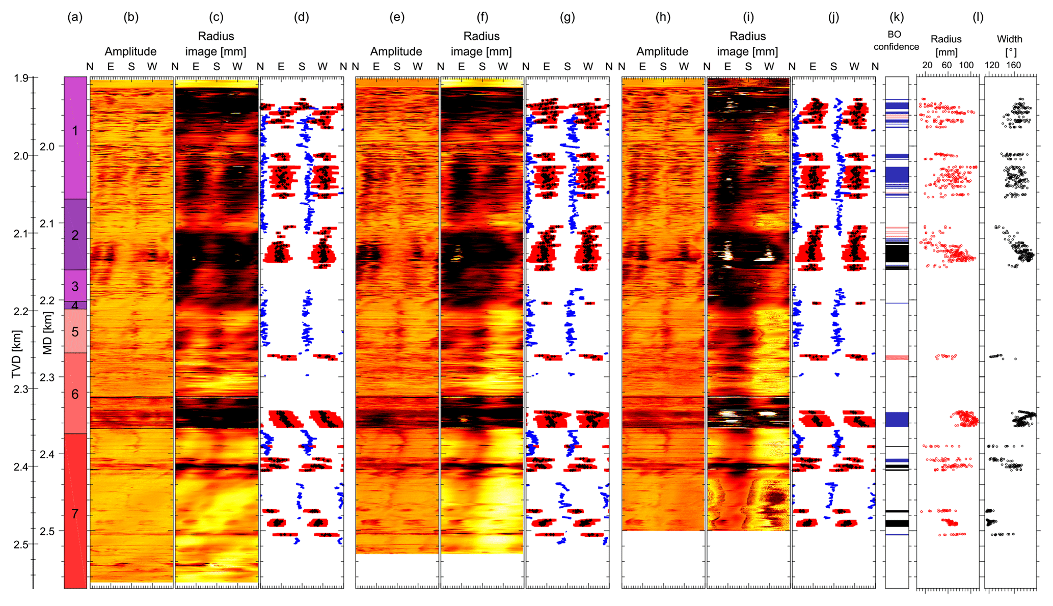
Figure 2 Synthesis of the data used in this analysis of borehole GRT-1. The measurements are expressed as a function of measured depth (MD) and vertical depth (TVD). (a) Simplified lithologic column: (1) Couches de Rehberg, (2) Couches de Trifels, (3) Annweiler sandstone, (4) Permian layers older than Annweiler sandstone, (5) rubefied granite, (6) hydrothermally altered granite and (7) low altered granite. The UBI images are presented, as are the data picked from the visual analysis of the double transit time image for the datasets for 2012 (b, c, d), 2013 (e, f, g) and 2015 (h, i, j) collected in GRT-1. The radius of the borehole computed from the double transit time image is displayed in panels (b)–(e) and (h). In panels (d)–(g) and (j), blue dots represent the azimuth of the drilling-induced tension fractures (DITFs), black dots represent the azimuth of the maximal radial depth of the breakouts and red bars represent the extension between the edges of the breakouts. Panel (k) presents information about the breakout (BO) confidence level applied to these results. Panel (l) summarizes the width (black dots; ^∘) and the enlargement radius (red dots; mm) measured in the 2012, 2013 and 2015 images.

3 Rittershoffen well data

3.1 GRT-1 data

Several extensive logging programs accompanied the drilling of wells GRT-1 and GRT-2. One was conducted in December 2012 in the open-hole section of GRT-1 a few days after drilling (Vidal et al., 2016). UBI acquisitions were carried out (Luthi, 2001). Figure 2b shows the amplitude image acquired in 2012 in GRT-1, and Fig. 2c displays the radius of the borehole computed from the double transit time image. The well logging also included caliper, spectral gamma ray and gamma–gamma acquisitions that enable an estimation of rock alteration and bulk density. The injectivity measured during the first hydraulic test between 30 December 2012 and 1 January 2013 showed a low injectivity (Baujard et al., 2017). To enhance the injectivity, the hydraulic connectivity between the well and the natural fracture network was increased through a multi-step reservoir development strategy. First, a thermal stimulation of the well was performed in April 2013. A cold fluid (12 ^∘C) was injected at a maximum rate of 25 L s⁻¹ with a maximum wellhead pressure of 2.8 MPa. The total injected volume was 4230 m³. Second, a chemical stimulation followed in June 2013. Using open-hole packers, a glutamate-based biocide was injected in specific zones of the open-hole section of GRT-1 (Baujard et al., 2017). Finally, a hydraulic stimulation of the well was performed in June 2013 with extensive seismic monitoring at the surface (Lengliné et al., 2017; Maurer et al., 2015). During these two last phases, a moderate-volume injection of 4400 m³ was injected in the open hole. The hydraulic stimulation lasted 30 h, with a major phase of stepwise flow rates from 10 to 80 L s⁻¹ (Baujard et al., 2017). As a result, the injectivity was improved fivefold due to this thermal, chemical and hydraulic (TCH) stimulation program. Two other borehole imaging programs were conducted in December 2013 shortly after stimulation of the well and significantly later in June 2015. The amplitude and travel time (or radius) images used in the analysis are respectively shown in Fig. 2e and f for the logging program in 2013 and in Fig. 2h and i for the logging program in 2015.

Table 1 Data acquired in GRT-1 and GRT-2 and the specificities of UBI acquisition programs.

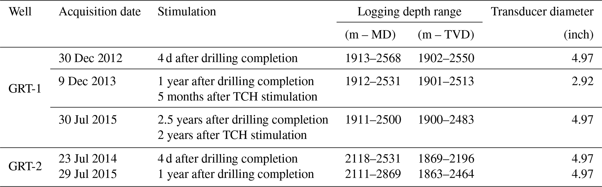
This time-lapse UBI dataset, whose characteristics are summarized in Table 1, provides the essential information for the present study as it enables us to identify evidence of irreversible deformation and failure (natural and induced fractures, breakouts, fault zones, damage zones, etc.) along the borehole wall. Vidal et al. (2016) analyzed the images acquired in GRT-1 and identified fractured zones impacted by the TCH stimulation without assessing the stress state and its evolution. Hehn et al. (2016), whose measurements are discussed later in Sect. 9.2, analyzed the orientation of drilling-induced tension fractures (DITFs) in GRT-1 in the granitic basement but also in the upper sedimentary layers, investigating the orientation of the stress field with depth.

We identify wellbore wall failure and use these observations to characterize the stress state in the reservoir, including its evolution in time. Wellhead pressure measurements of the hydraulic stimulation are also used to estimate a lower bound of the minimum horizontal stress (S_h).

3.2 GRT-2 data

An extended logging program was also conducted in GRT-2, including repeated UBI borehole imaging (see Table 1). Figure 3c and d respectively show the amplitude image acquired in 2014 between 2404 and 2412 m and the radius image acquired in 2015 between 2468 and 2472 m in GRT-2. No hydraulic stimulation was performed in this well since its initial injectivity was sufficient (Baujard et al., 2017).

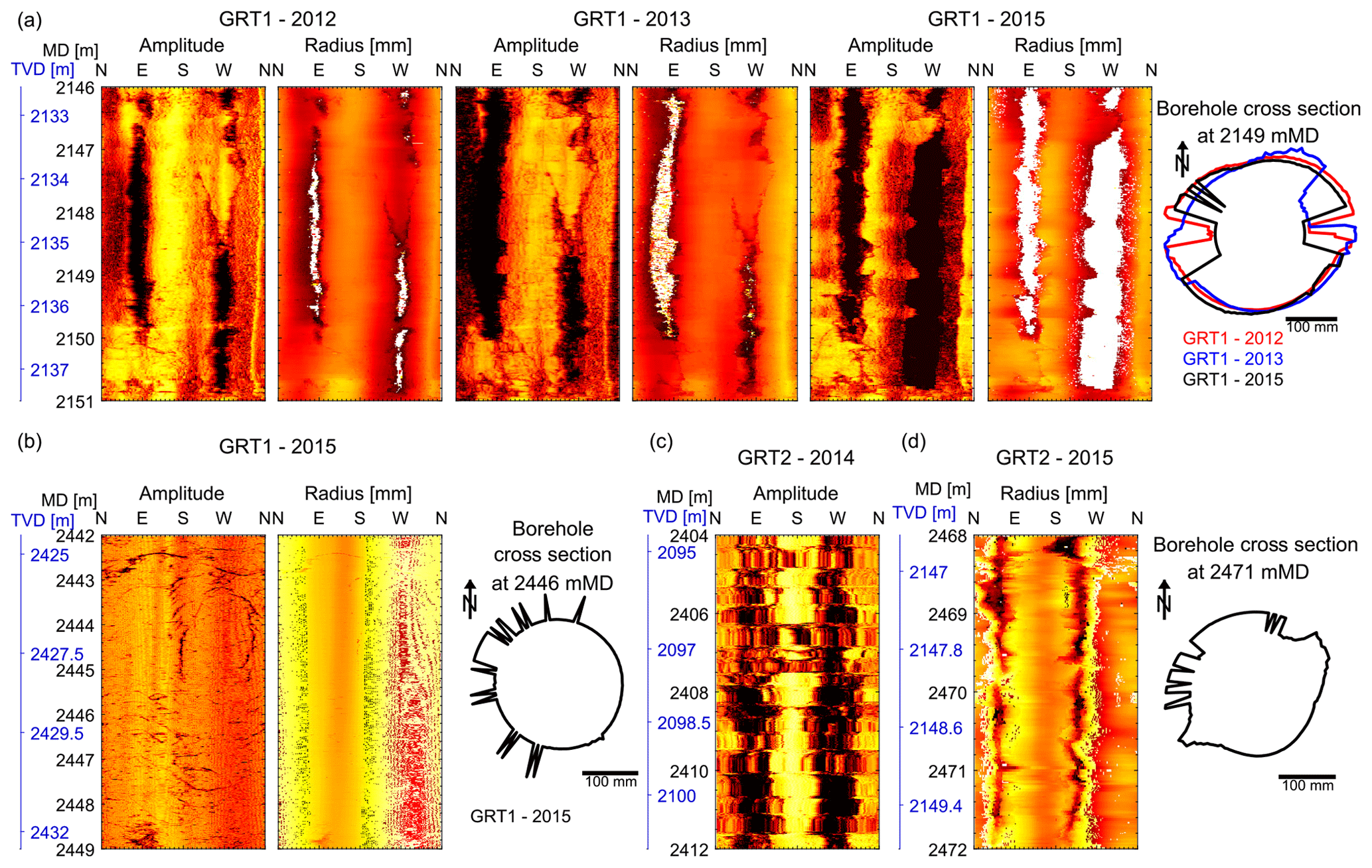
Figure 3 Example of image artifact observed on the GRT-1 and GRT-2 dataset. (a) Comparison of data from 2012, 2013 and 2015 collected in GRT-1 presenting a signal loss artifact in sandstones, clearly highlighted by persisting white patches in the radius signal. (b) Processing noise resembling wood grain textures, visible on the 2015 GRT-1 image both on the amplitude and radius image in granite. (c) Alternating compression and stretching of the image characteristic of stick-slip artifacts, highlighted along the entire GRT-2-2014 image. (d) Erroneous radius record observable on the GRT-2-2015 image in granite, possibly related to tool decentralization.

4 Stress estimation methodology

The approaches proposed by Zoback et al. (2003) and by Schmitt et al. (2012) are used to fully characterize the in situ stress field at the Rittershoffen geothermal project. In the following, the symbol S refers to the total stress, while σ refers to the effective stress (Jaeger and Cook, 2009). We suppose that one of the principal stresses of the in situ stress tensor is vertical, which is a common assumption. This hypothesis is justified by the first-order influence of gravity on the in situ stress state, although this assumption may not be valid locally. Moreover, no “en échelon” patterns are highlighted in GRT-1 or GRT-2, which would be the case if the direction of any of the principal stresses differs from the well inclination by more than 20^∘, as was observed, for example, by Wileveau et al. (2007) in highly deviated wells. We show that the breakouts measured in GRT-1 are collinear with the borehole axis, which confirms that the vertical direction is principal. In the following, we denote the vertical principal stress S_v. The magnitude of the vertical stress S_v is obtained from the weight of the overburden. It is calculated by the integration of density logs (see Sect. 8.2). The two other principal stresses act horizontally: S_H, the maximum horizontal stress, and S_h, the minimum horizontal stress. The magnitude of the minimum horizontal stress S_h is estimated from the wellhead pressure measurements carried out during the hydraulic stimulation of GRT-1 and from the hydraulic tests performed in the reservoir of Soultz-sous-Forêts (see Sect. 8.3). The analysis of the borehole failures is evaluated using televiewer image data (Zemanek et al., 1970; Zoback et al., 1985). The orientation and magnitude of S_H are assessed using a failure condition at the borehole wall with the three common failure criteria considered in our analysis, i.e., the Mohr–Coulomb criterion (Jaeger and Cook, 2009), the Mogi–Coulomb criterion (Zimmerman and Al-Ajmi, 2006) and a true triaxial version of the Hoek–Brown criteria (Zhang et al., 2010), and are presented in Sect. 4.2.

4.1 Wellbore stress concentration

To express the stress concentration around the quasi-vertical borehole GRT-1 (maximum deviation is only about 9^∘), we assumed its shape to be a cylindrical hole and used the well-known linear elastic solution, often referred to as the Kirsch solution (Kirsch, 1898; Schmitt et al., 2012). For the deviated well GRT-2 where the plane strain approximation is no longer valid, we used a 3-D solution taking into account the constant deviation of 37^∘ measured along the section of interest. The equations that involve the geometry parameters of the well, the far-field stresses and the fluid pressure are well documented in the literature. We refer to the summary proposed in the review from Schmitt et al. (2012) for the general case of a 3-D well randomly inclined in regard to the far-field stresses. The same methodology has been, for example, proposed by Wileveau et al. (2007). A summary of the steps leading to the equations used to compute the S_H stresses for the deviated well GRT-2 is presented in Appendix A. Note that we included in our solution a thermal stress component that accounts for the thermal perturbation induced by the drilling process. This component is detailed later in Sect. 8.4. We used the formulation of the thermo-elastic stresses arising at a borehole given by Voight and Stephens (1982), also recalled in Schmitt et al. (2012). We computed the effective stress at the borehole wall considering a hydrostatic pore pressure given by $P_{\mathrm{p}}={\mathit{\rho }}_{\mathrm{f}}\cdot g\cdot z$, i.e., with the head level located at the surface. The fluid density ρ_f is taken as 1000 kg m⁻³ and the gravitational acceleration g as 9.81 m² s⁻¹; z is the vertical depth (TVD) in meters from the ground surface.

4.2 Failure criterion

At the scale of the surroundings of the borehole (a few decameters), we assume a linear elastic, homogeneous and isotropic rock behavior prior to failure. When the maximum principal stress exceeds the compressive rock strength, rock fails in compression (Jaeger and Cook, 2009). Failure at the borehole wall is assessed using the elastic stress concentration solutions presented in Sect. 4.1, combined with an adequate failure criterion. There is currently no consensus concerning the appropriate failure criteria to assess wellbore wall strength. In the case in which the pore pressure and the internal wellbore pressure are in equilibrium, the radial effective stress at the borehole wall is equal to zero, so a common assumption is to consider the uniaxial compressive strength (UCS) to be a good estimate of wellbore strength (Barton et al., 1988; Zoback et al., 2003). Others suggest that the strength of borehole walls in low-porosity brittle rocks could be less than the UCS because the failure could be controlled by extensile strains (Barton and Shen, 2018; Walton et al., 2015) or fluid pressure penetration (Chang and Haimson, 2007). The presence of nonzero minimum principal stress and the strengthening effect of the intermediate principal stress, however, suggest that the borehole wall strength should be larger than the UCS (Colmenares and Zoback, 2002; Haimson, 2006; Mogi, 1971). In view of this situation and because stress magnitude evaluation differs according to the criterion used in the analysis, we compared the estimates obtained with three commonly used failure criteria in borehole breakout analyses: (1) the Mohr–Coulomb criterion (Jaeger and Cook, 2009), (2) the Mogi–Coulomb criterion (Zimmerman and Al-Ajmi, 2006) and (3) a true triaxial version of the Hoek–Brown criteria (Zhang et al., 2010). The formulation is given in Eq. (1) for the Mohr–Coulomb criterion in the principal effective stress space σ₁–σ₃. The Mogi–Coulomb and Hoek–Brown criteria include a so-called “effective mean stress” (Zimmerman and Al-Ajmi, 2006) expressed as a function of the principal effective stresses as ${\mathit{\sigma }}_{\mathrm{m}}=\frac{{\mathit{\sigma }}_{\mathrm{1}}+{\mathit{\sigma }}_{\mathrm{3}}}{\mathrm{2}}$ and an octahedral shear stress given by ${\mathit{\tau }}_{\mathrm{oct}}=\sqrt{{\left({\mathit{\sigma }}_{\mathrm{1}}+{\mathit{\sigma }}_{\mathrm{2}}\right)}^{\mathrm{2}}+{\left({\mathit{\sigma }}_{\mathrm{2}}+{\mathit{\sigma }}_{\mathrm{3}}\right)}^{\mathrm{2}}+{\left({\mathit{\sigma }}_{\mathrm{3}}+{\mathit{\sigma }}_{\mathrm{1}}\right)}^{\mathrm{2}}}$. Equations (2) and (3) express the Mogi–Coulomb and Hoek–Brown criteria in the space (τ_oct, σ_m).

Mohr–Coulomb

$$\begin{array}{}\text{(1)}& {\mathit{\sigma }}_{\mathrm{1}}\ge C_{\mathrm{0}}+q\cdot {\mathit{\sigma }}_{\mathrm{3}}\end{array}$$

Mogi–Coulomb

$$\begin{array}{}\text{(2)}& {\mathit{\tau }}_{\mathrm{oct}}\ge a+b\cdot {\mathit{\sigma }}_{\mathrm{m}}\end{array}$$

Hoek–Brown

$$\begin{array}{}\text{(3)}& {\displaystyle \frac{\mathrm{9}}{\mathrm{2}.C_{\mathrm{0}}}}\cdot {\mathit{\tau }}_{\mathrm{oct}}^{\mathrm{2}}+{\displaystyle \frac{\mathrm{3}}{\mathrm{2}\sqrt{\mathrm{2}}}}\cdot m_i\cdot {\mathit{\tau }}_{\mathrm{oct}}-m_i\cdot {\mathit{\sigma }}_{\mathrm{m}}\ge C_{\mathrm{0}}\end{array}$$

C₀ is the uniaxial compressive strength and q is a material constant that can be related to the internal friction angle, φ, through $q=\left(\frac{\mathit{\pi }}{\mathrm{4}}+\frac{\mathit{\phi }}{\mathrm{2}}\right)$. The variables a and b in the Mogi–Coulomb criteria and m_i in the Hoek–Brown criteria are parameters that are related to material friction and cohesion.

Table 2 Elastic (Poisson ratio) and strength parameters (used in the Mohr–Coulomb, Mogi–Coulomb and Hoek–Brown failure criteria) for the four geological units retained in the model, for both the GRT-1 and GRT-2 wells, as a function of measured depth (MD) and vertical depth (TVD). Elastic and strength parameters for granites are based on a data compilation of tests conducted on samples from Soultz-sous-Forêts. For the Buntsandstein sandstones, we use the usual strength parameters based on Hoek and Brown (1997).

5 Strength estimation

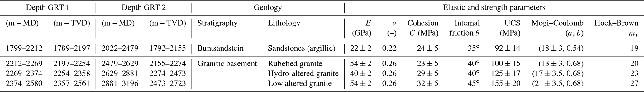
Four simplified lithological categories have been used for the strength characterization of the rock at depth in the Rittershoffen reservoir. The open-hole section of GRT-1 and GRT-2 crosses Vosges sandstones and Annweiler sandstones of the Buntsandstein. All the lower Triassic sandstones have been grouped in a single category. The granitic section has been separated in three categories according to the type and intensity of alteration. The simplified lithologic profile for the GRT-1 and GRT-2 wells is indicated in Table 2. Considering the methodology used here, the relevance and accuracy of the stress characterization are highly conditioned by the values of the rock strength parameters and by the failure criterion chosen. In Rittershoffen, the drilling was performed exclusively in destructive mode and no sample is available to measure rock moduli and strength characteristics. The GRT-1 and GRT-2 wells penetrate geologic units similar to those in the nearby Soultz-sous-Forêts site. Information from the Soultz-sous-Forêts site is thus used to better characterize the strength and mechanical characteristics of the geological units through which the wells in Rittershoffen are drilled (Heap et al., 2017, 2019; Kushnir et al., 2018; Villeneuve et al., 2018). Mechanical tests that have been carried out on core samples from the Soultz-sous-Forêts site are used to characterize the rock properties (Rummel, 1991; Valley and Evans, 2006). At the Soultz-sous-Forêts site, the EPS-1 borehole was continuously cored from 930 to 2227 m (Genter et al., 2010; Genter and Traineau, 1992, 1996), providing samples of the sandstones in the Buntsandstein and in the crystalline basement. Some cores have also been obtained in borehole GPK-1 from various depth sections and were analyzed by Rummel (1991). For the Buntsandstein sandstones, Heap et al. (2019) studied in detail the strength evolution with depth of the Buntsandstein mechanical properties. They identified significant variations of the compressive strength together with elastic modulus changes. They also pointed out the role of the fluid content in the UCS. However, these variations are limited compared to the statistical fluctuations of our measurement. Accordingly, we gathered the Buntsandstein sandstones as a single unit. The elastic and strength parameters used for our analyses are summarized in Table 2. The variability range given for elastic parameters, cohesion and UCS reflects natural rock heterogeneities and depicts the variability in values encountered. Indeed, we recognize different sources of uncertainty on the mechanical and strength parameters which limit our approach. In addition to the absence of direct strength measurements for the study site, the mechanical and strength parameters are selected from core or cutting analyses performed in laboratory conditions. The parameters are thus not necessarily representative in situ under large-scale conditions due to, for example, the presence of core damage.

6 Images processing and borehole failure identification

Stress-induced failures are identified and measured from acoustic borehole images. The confidence and accuracy of these determinations depend on the quality of the images. In the following, we describe the original data as well as the processing we applied to improve the quality and comparability of the images. We also explain how we measure borehole failure on these images and the limitations associated with these measurements.

6.1 Quality of the acoustic televiewer images

Several artifacts can deteriorate the quality of acoustic image data (Lofts and Bourke, 1999). The images acquired in Rittershoffen suffer from some of these limitations. The quality of the image depends of the tool specification, the acquisition parameters and logging conditions. All acoustic images at Rittershoffen were acquired by Schlumberger with their UBI (ultrasonic borehole imager) tool. The tool and acquisition parameters were similar between each log but not identical. For example, the GRT-1 log in 2013 was acquired using a smaller acquisition head (see the changes in transducer diameter detailed in Table 1). The acquisition resolution was the same for every log, i.e., 2^∘ azimuthal resolution and 1 cm depth sampling step.

The 2012 log of GRT-1 has the best-quality image of the entire suite. The image suffers from a signal loss artifact (Lofts and Bourke, 1999) in some limited sections, most commonly related to the presence of breakouts or major fracture zones. The zones of signal loss are clearly identified in the radius image presented in Fig. 3a by persisting white patches.

The 2013 log of GRT-1 is of comparable quality as the 2012 log and also suffers from some limited signal loss artifacts. The major issue with the image of GRT-1 acquired in 2013 is that the orientation module was not included in the tool string, and thus the image cannot be oriented with magnetometer data as is usually done for this type of data.

The 2015 log of GRT-1 generally suffers from signal loss issues, not only in areas with major fracture zones and breakouts. In the lower part of the log, wood grain textures (Lofts and Bourke, 1999) related to processing noise are also observable (see Fig. 3b). Wood grain textures are especially encountered below 2431 m MD.

The quality of log data from GRT-2 is generally lower than for GRT-1. This is due to the deviation of GRT-2 that makes wireline logging more difficult. The 2014 log of GRT-2 suffers from stick-slip artifacts on its entire length. The effects of the alternating compression and stretching on the images highlighted in Fig. 3c are particularly significant and possibly lead to errors in the recording of the fractures. The 2015 log in GRT-2 does not show any sign of stick-slip but presents an erroneous borehole radius record, leading to an incorrect borehole geometry assessment (Fig. 3d).

Despite these difficulties, the images collected in the GRT-1 borehole are of excellent quality. Signal loss is the main problem and it prevents us from measuring the depth in the radial direction of the breakout in some zones. Given the extent of the artifacts highlighted in GRT-2, the measurements of the breakout parameters in this borehole are much more uncertain.

6.2 Processing of the UBI images

Prior to the use of the images for assessing borehole failure, the images went through the following preprocessing steps:

1. transit time was converted to radius using the fluid velocity recorded during the probe trip down the borehole;

2. images were filtered to reduce noise; and

3. digital image correlation was applied across the successive logs in order to correct the image misalignment both in azimuth and depth.

The borehole radius was computed from the transit time following Luthi (2001):

$$\begin{array}{}\text{(4)}& r={\displaystyle \frac{t_{\mathrm{twt}}\cdot v_{\mathrm{m}}}{\mathrm{2}}}+d,\end{array}$$

with t_twt the two-way travel time, v_m the acoustic wave velocity in the drilling mud and d the logging tool radius. Images are filtered using a selective despiking algorithm implemented in WellCad^™ using a cutoff high level (75 %) and a cutoff low level (25 %) in a 3×3 pixel window. The goal of this process is to replace outliers by cutoff values when the radius exceeds the cutoff high or low level. Finally, digital image correlation was used to ensure proper alignment of the UBI images. This was required for the GRT-1 2013 image because this image was not oriented with a magnetometer–accelerometer tool. The process was also applied to the 2015 GRT-1 data to facilitate comparison between images. For this purpose, we developed a technique based on a particle image velocimetry (PIV) method (Thielicke and Stamhuis, 2014) that relies on optical image correlation but being applied to travel time UBI images. This image alignment process is illustrated in Fig. 4. Figure 4a shows, as an example, the “correlation box” in the travel time UBI image of reference – i.e., 2012 in this case – and the corresponding one in the image to compare with – i.e., the image of 2013 – which is shifted for a given displacement vector (dX, dY) within the “search box”. The cross-correlation function, which is a measure of the similarity between the thumbnails, is computed between the correlation boxes for each displacement vector (dX, dY). Figure 4a shows a map of the cross-correlation function computed for every displacement vector in a given search box. The two-dimensional cross-correlation function is an operator acting on two intensity functions, s(X,Y) and r(X,Y), defined as a norm of the color levels at each position of each thumbnail. C_sr is defined at a position (X,Y) and for a shift (dX, dY) by Eq. (5).

$$\begin{array}{}\text{(5)}& \begin{array}{rl}{C}_{\mathrm{sr}}\left(\mathrm{d}\mathit{X},\mathrm{d}\mathit{Y}\right)& =s\left(X,Y\right)\otimes r\left(X,Y\right)\\ & =\underset{-\mathrm{\infty }}{\overset{+\mathrm{\infty }}{\iint }}s\left(X,Y\right)r\left(X-\mathrm{d}\mathit{X},Y-\mathrm{d}\mathit{Y}\right)\mathrm{d}\mathit{X}\mathrm{d}\mathit{Y}\end{array}\end{array}$$

The position (dX, dY) within the search box with the highest cross-correlation corresponds to the best alignment (see Fig. 4a). The operation is repeated along the image for each position of the search box. Importantly, the correlation box is taken with an anisotropic shape to account for the rigid rotation of the UBI tool and the linear property of the acoustic camera. The size of the correlation box is 180×20 pixels. This configuration is appropriate to principally identify the azimuthal offset, while it is less sensitive to the depth mismatch. We investigated offset up to 180 pixels horizontally, corresponding for our 2^∘ resolution to a complete 360^∘ rotation. We considered a vertical offset of ±10 pixels, corresponding to offsets of about ±10 cm. Figure 4b gives an example of image realignment and shows the efficiency of the process. This correlation process allows us to finely align the successive images and thus to study the borehole shape evolution with time more accurately.

Figure 4 (a) Sketch presenting the process used to orient the images of GRT-1. A correlation box is defined in the double transit time image of reference (acquired in 2012) and is progressively shifted in the image to compare with (red windows) within the limits of the search box (black window). We compute the correlation between the correlation box in its initial position in the image of reference and the shifted correlation box in the image to compare with for each position (right insert). The displacement maximizing the correlation factor enables, at a given depth, us to rotate and adapt the image of 2013 and 2015 according to the image of 2012. (b) Example of original and reoriented time transit images of 2013 at a depth of 2414 m (TVD) in GRT-1.

6.3 Determination of the borehole failure

For GRT-1, the breakouts have been determined through a visual analysis of borehole sections computed every 20 cm from 1926 to 2568 m (MD) from the double transit time data. The borehole sections are computed by stacking (averaging using the median) the data collected every 1 cm over 20 cm borehole intervals (with no overlap between two successive sections). The median is thus used because it is less sensitive to extreme values than the mean and is thus efficient at removing local noise from the data. Prior to determining breakout geometrical parameters, the actual borehole center is determined by adjusting the best-fitted ellipse to the borehole section. This process corrects for eventual logging probe decentralization. For each section presenting the characteristic elongated shape of breakouts due to stress-induced failure, the azimuthal position of the edges and the center of each limb are determined by visual inspection. Figure 5 gives examples of such a determination to depict the process. The breakout edges are defined as the location where the wellbore section departs from a quasi-circular section adjusted by the best-fitted ellipse. As can be seen in Fig. 5, this typically spans an azimuthal range much broader than the low-amplitude reflections visible as dark bands on the amplitude images and justifies the choice to use the double transit time data. The positions of the breakout edges are not easy to determine in a systematic and indisputable manner, and significant uncertainty is associated with these measurements. Related to this issue, it is not possible to determine on the images what azimuthal range of the wellbore is enlarged by purely stress redistribution processes and what part is enlarged subsequently by the effects of drill string wear. These uncertainties about the physical process controlling the enlargement of the breakout could limit the comparisons between the three successive logs acquired in GRT-1. Breakout measurements were thus performed on all three images concomitantly and consistently. We ensured, for example, that within a tolerance dictated by the uncertainties of the measurements, the width of breakouts only remains identical or increases: no decrease in width is measured between successive logs.

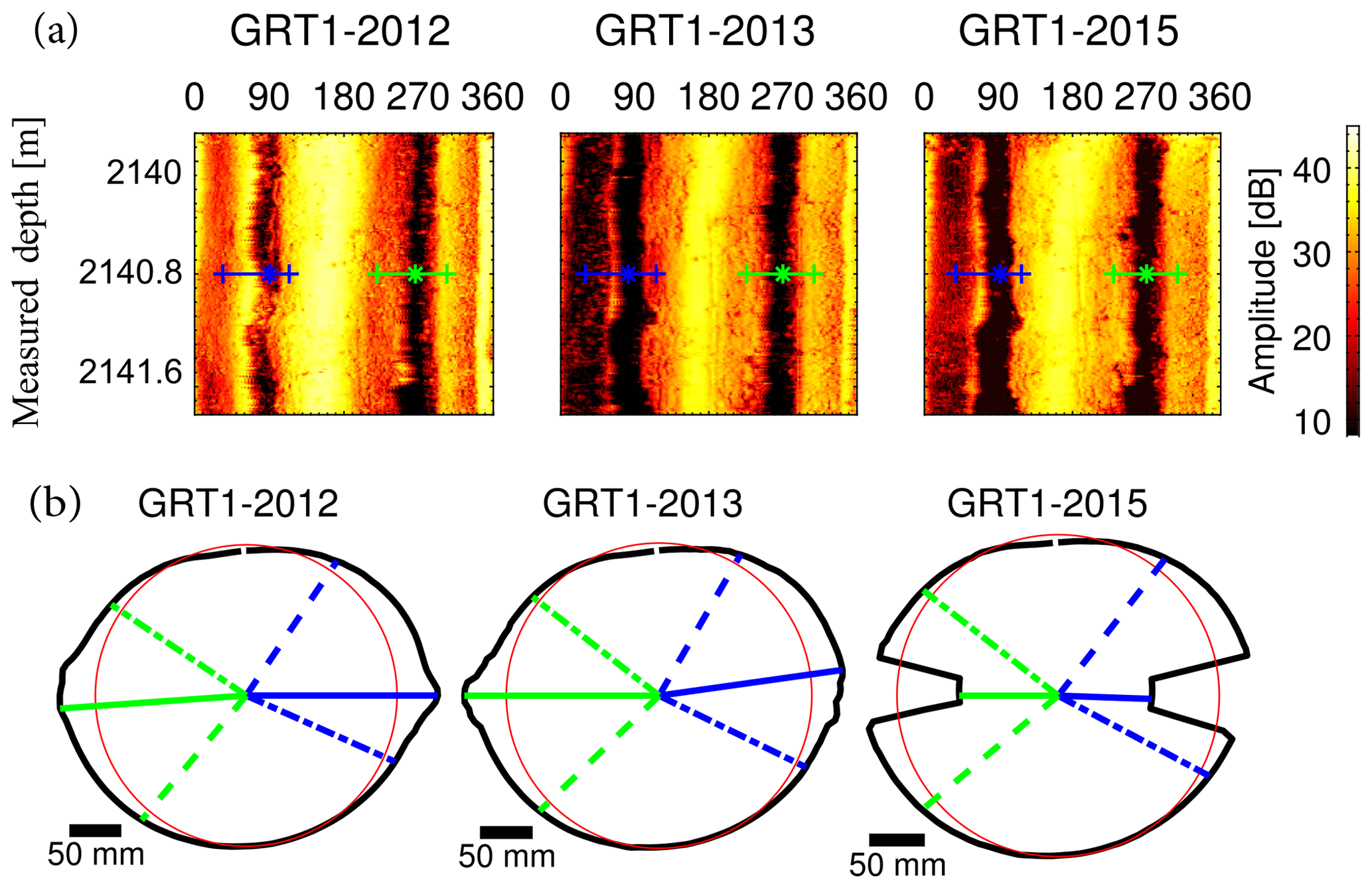
Figure 5 Example of breakout geometry determination in sandstones. (a) Amplitude images for GRT-1 at 2140.8 m for the logs from 2012, 2013 and 2015. (b) Wellbore section at 2140.8 m computed from the transit time images from the 2012, 2013 and 2015 logs, respectively. The breakout extent is determined on the wellbore section. The blue and green dashed lines represent the extent of the breakout, while the plain lines represent the azimuth of the maximum radial extension of the breakout.

Figure 2d, g and j summarize all the measurements of the breakout geometry performed in GRT-1 for the images acquired in 2012, 2013 and 2015. Black dots indicate the azimuth at which the radius of the breakout is maximum and red bars link the azimuthal position of the breakout edges used to compute the width of the breakouts. Given the difficulty of measuring breakouts as discussed previously (i.e., artifacts affecting the images, disputable positions of the breakout edges), a confidence ranking has been established for each breakout. This confidence level is presented in Fig. 2k. From the geometry of the breakouts, we compute the breakout widths which are obtained from the breakout edge azimuths. The deepest point of the breakout is used to determine the enlargement radius. In some situations, signal loss issues prevent the determination of the enlargement radius, as shown in Fig. 5 for the image of GRT-1 acquired in 2015. The measured width (black dots; in degrees) and enlargement radius (red dots; mm) are determined from the GRT-1 dataset acquired in 2012 and presented in Fig. 2l.

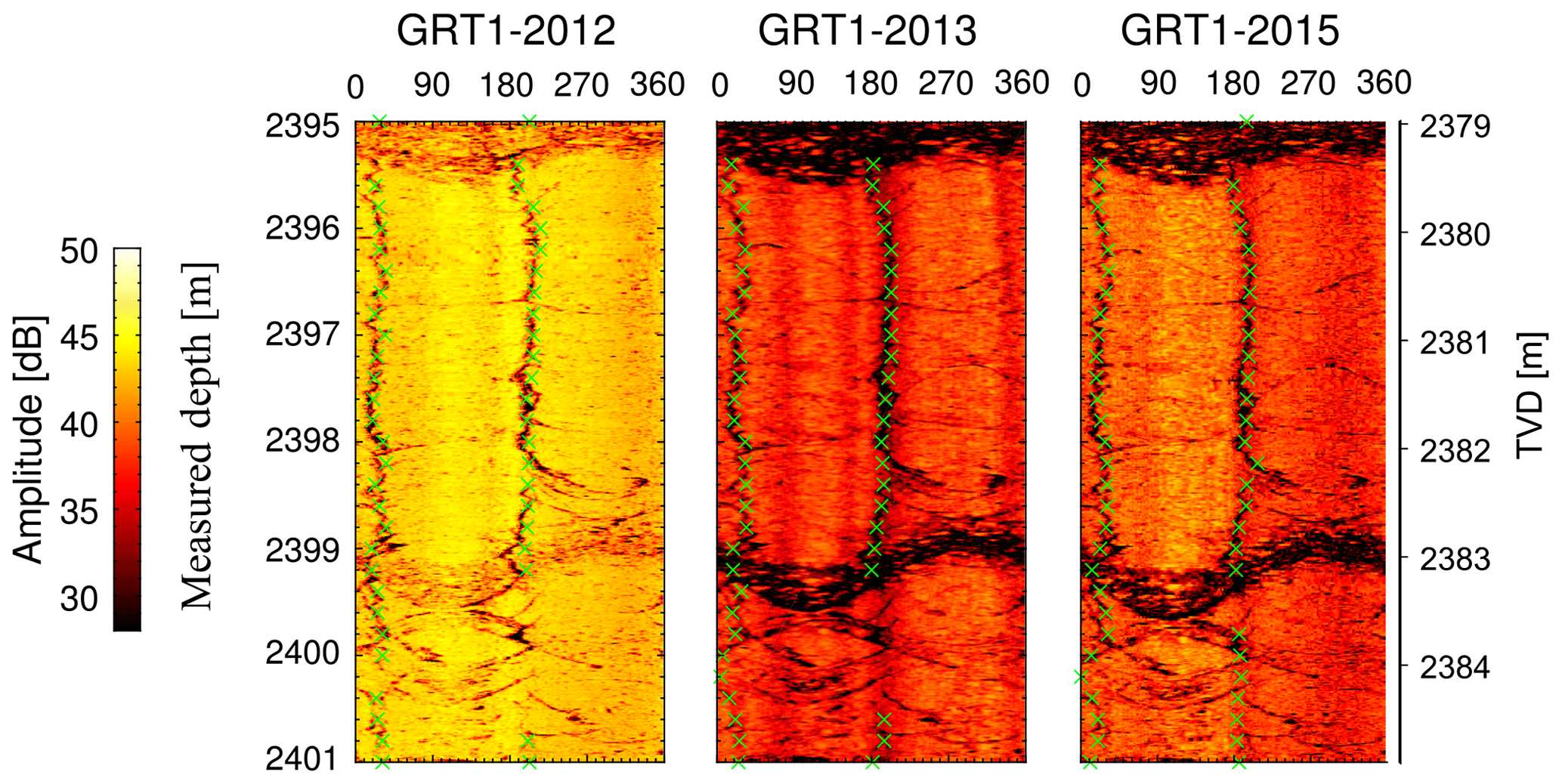
Figure 6 Examples of drilling-induced tension fractures (DITFs) observed in the granitic section of GRT-1 in the amplitude images acquired in 2012, 2013 and 2015. The azimuth of the DITFs is measured every 20 cm (green crosses).

Drilling-induced tension fractures (DITFs) are also identified from the GRT-1 borehole images using the same procedure as for the breakout determination. For example, clear DITFs are evident in the amplitude image from 2395 to 2400 m in GRT-1 and presented in Fig. 6. Green crosses show the azimuth of the DITFs measured in GRT-1 every 20 cm. Blue dots in Fig. 2d, g and j summarize the azimuth of the DITFs measured in GRT-1 in 2012, 2013 and 2015, respectively. Given the poor quality of the double transit time images acquired in GRT-2, less focus has been given to the analysis of the borehole failure in this well. The dataset consists of the acquisitions made in 2014 after completion of the borehole and in 2015. The investigated depths vary from the 2014 to the 2015 dataset. The depth is from 1950 m (vertical depth – 2220 m MD) down to 2125 m (TVD – 2440 m MD) in 2014, while it is down to 2160 m (TVD – 2480 m MD) in 2015. The well is strongly deviated. The concentration of stresses within the borehole wall is expressed under the assumption of a constant deviation of 37^∘, and measurements are carried out as a function of the true vertical depth to be comparable with the results obtained in GRT-1, which is considered to be vertical. Borehole sections are computed every 50 cm. To this end, borehole sections are stacked using the data collected every 1 cm over 50 cm borehole intervals, all along the transit time image. As for GRT-1, the actual borehole center is determined by adjusting a best-fitted ellipse to the borehole section. Breakouts are analyzed by visual analysis in the same manner as for GRT-1 data. The difficulties encountered with the identification of breakout geometry are more pronounced for images acquired in GRT-2, as artifacts are more developed. The deviation of this well results in pronounced stick-slip effects. For a more accurate comparison between the measurements carried out on the images acquired in 2014 and 2015, measurements are performed for the two images concomitantly. No DITFs are identified on the GRT-2 borehole images.

7 Analyses of temporal borehole failure evolution

The characterization of the stress tensor derived from the analysis of borehole failures typically relies on a single borehole image dataset. From this snapshot in time, stresses are estimated, while information on the evolution of breakout shape in time is not available. Interestingly, for the ECOGI project, the acquisition of three successive image logs allows us to study this evolution. Here, the time evolution of breakouts, referred to as breakout development, is analyzed to characterize the time evolution of the borehole failure. A common hypothesis concerning borehole breakout evolution is that breakout width remains stable and is controlled by the stress state around the well at the initial rupture time. Progressive failure is assumed, however, to lead to breakout deepening until a stable profile is reached (Zoback et al., 2003).

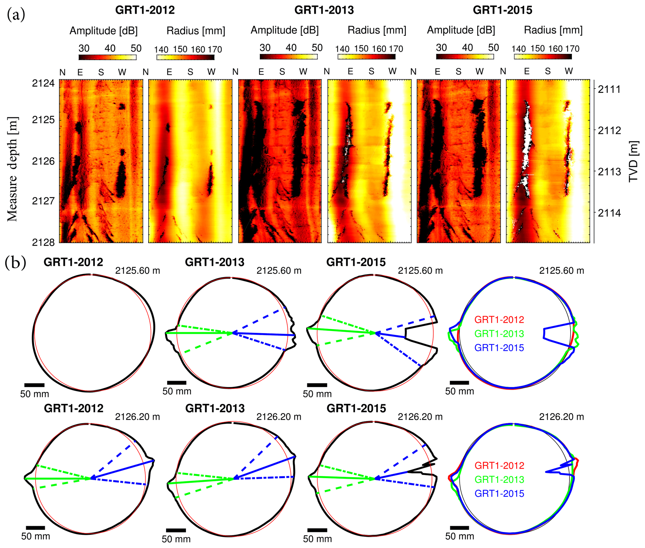
Figure 7 Examples of breakout shape evolution between the three successive images collected in GRT-1 in sandstones. (a) The amplitude images and the radius computed from the time transit images for a section of GRT-1 from 2124 to 2128 m (MD) in 2012, 2013 and 2015. (b) The mean section computed at 2125.6 and 2126.2 m (MD) from the time transit images averaged over 60 cm intervals. The sections are represented along with an 8.5 inch radius circle representing the unaltered open-hole section. The sections from the images of 2012, 2013 and 2015 are superposed on the far right of panel (b).

An example of a time-lapse comparison of breakout shapes is presented in Fig. 7. Images of GRT-1 from 2012, 2013 and 2015 show a clear breakout at a depth of about 2126 m in the Couches de Trifels in the Buntsandstein. Breakouts can present three types of evolution.

1. They can develop along the well, corresponding to an increase in the vertical length of breakouts. We refer to this process as breakout extension.

2. They can widen, corresponding to an apparent opening between the edges of the breakouts. We refer to this process as breakout widening.

3. They can deepen, corresponding to an increase in the maximal radius of the breakout (or “depth” of the breakout) measured in the borehole cross section at a given depth. We refer to this process as breakout deepening.

Figure 7 shows the evolution from 2012 to 2015 of the breakouts at 2125.6 m. Failure did not occur in 2012, while breakouts are visible in 2013 and 2015. When superposing the 2013–2015 borehole sections, no change in breakout shape is highlighted for the west limb although a slight widening is visible on the east limb. Possible deepening of the east limb is occulted by signal loss issues. The borehole section computed at 2126.2 m shows, in contrast, no modification of the breakout shape from 2012 to 2015 in GRT-1.

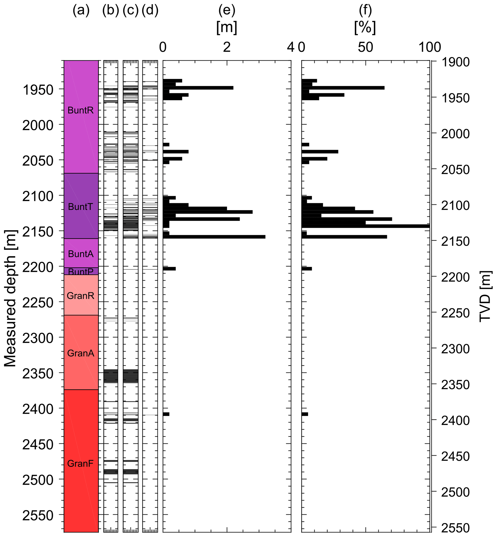
Figure 8 Development of breakouts along the GRT-1 borehole between 2012 and 2013. (a) Simplified lithologies along the GRT-1 borehole as a function of measured depth (MD) or vertical depth (TVD). BuntR stands for Couches de Rehberg, BuntT for Couches de Trifels, BuntA for Annweiler sandstone, BuntP for Permian layers older than Annweiler sandstone, GranR for rubefied granites, GranA for hydrothermally altered granite and GranF for low altered granite. The major fault zone crossing GRT-1 at 2368 m is represented as a black band. (b) Breakout positions in GRT-1 in 2012. (c) Breakout positions in GRT-1 in 2013. (d) Intervals at which breakouts are present in 2013 but not in 2012. (e) Breakout length increase (m) along the borehole between 2012 and 2013 in 5 m bins. (f) Fraction (%) of wellbore length that was free of a breakout in 2012 but presents a breakout on the 2013 image, computed in 5 m bins.

The development of borehole failures also depends on the lithology. Breakout extension (longitudinal failure development) is quite common in the Buntsandstein, while it is very limited in the basement granites, which is highlighted in Fig. 8. The evolution occurs exclusively between the 2012 and 2013 datasets, while no longitudinal extension occurs during 2013 and 2015. In 2012, a total breakout length of 404 m is observed. It increases to 504 m in 2013 and then remains stable in 2015 with a length of 506 m. There is no clear evolution of DITFs along the GRT-1 well despite the hydraulic and thermal stimulation performed between 2012 and 2013.

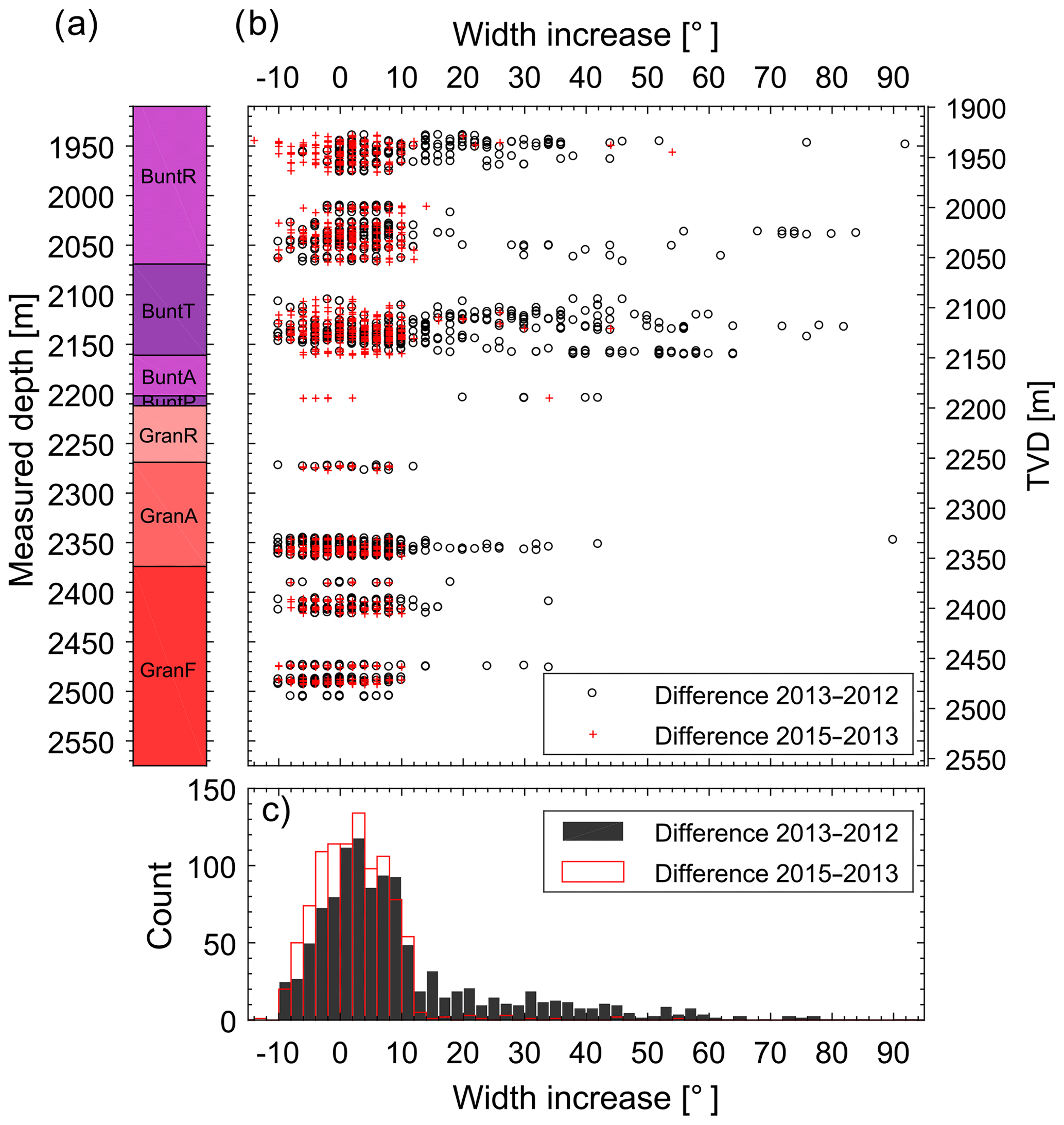
Figure 9 Evolution of breakout width in the GRT-1 borehole as a function of measured depth (MD) or vertical depth (TVD). (a) Simplified lithologies along the GRT-1 borehole (see Fig. 8 for the legend). (b) Width increase between the 2012–2013 time interval (black circles) and the 2013–2015 time interval (red crosses) presented as a function of the vertical depth. (c) Histograms in 2^∘ classes of breakout width changes for the 2012–2013 interval (black) and the 2013–2015 interval (red).

Figure 9 shows an increase in breakout width. We first compare the data acquired in 2012 and in 2013; 73 % of the change of width is within an interval −10^∘ ∕ +10^∘, i.e., within our measurement uncertainty. For these breakouts no changes in width can be highlighted within our level of uncertainty. However, for 27 % of our data, we observe an increase in width larger than 10^∘. This is reflected by the long tail (with values higher than 10^∘) of the histogram computed from the width of breakouts (see Fig. 9c). The widening of these breakouts is undisputable. When comparing the data acquired in 2013 and in 2015, very few changes are observed. Indeed, most of the measured changes remain below our uncertainty level of ±10^∘ (red histogram in Fig. 9c).

The evolution of the maximum radial extension (breakout deepening) of the breakout measured in the borehole cross sections is presented in Fig. 10. This parameter is more delicate to track because of signal loss issues (see, for example, Fig. 3a). In our analysis, we filtered out obvious incorrect depth measurements related to these artifacts, i.e., when the computed radius from the transit time image is clearly shorter than the drill bit radius. For both time intervals (2012–2013 and 2013–2015), the change in the depth of the breakout is symmetrically distributed around 0 mm and spans a variability of about ±15 mm. We interpret this distribution as an indication that if any deepening occurred, it remained within our uncertainty level. Our data analysis does not enable us to draw the conclusion of a general deepening of the breakouts.

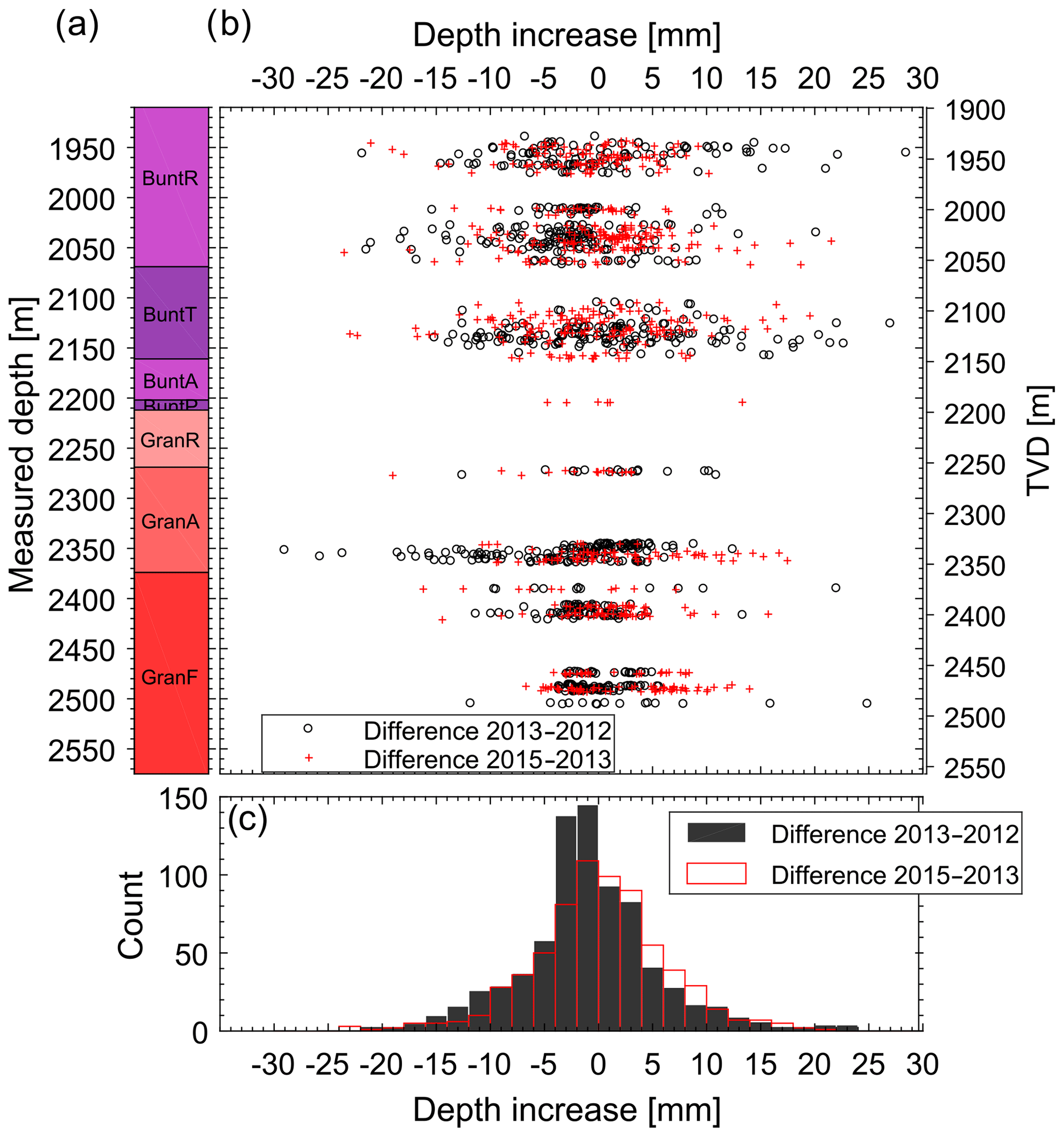
Figure 10 Evolution of the depth of the breakouts in the GRT-1 borehole as a function of measured depth (MD) or vertical depth (TVD). (a) Simplified lithologies along the GRT-1 borehole (see Fig. 8 for the legend). (b) Increase in the maximum radial extension between the 2012–2013 time interval (black circles) and 2013–2015 time interval (red crosses) presented as a function of depth. (c) Histograms in 2 mm classes of breakout width changes for the 2012–2013 interval (black) and 2013–2015 interval (red).

8 Stress characterization

We propose in this section a complete stress characterization at different periods in both the GRT-1 and GRT-2 wells, including a thermal history and thermal stress analyses, and discuss the impact of breakout widening in time on stress estimation. To that purpose, we first determine the orientation of the stress tensor. We then detail how we estimate the minimum horizontal stress component S_h, the vertical stress component S_v and the thermal component. Finally, we propose an estimation of the maximum horizontal stress component S_H from the measurement of the width of breakouts.

8.1 Maximum horizontal stress S_H orientation

The orientations of breakouts and DITFs are a direct measure of the principal stress directions in a plane perpendicular to the well. As discussed previously, we assume that S_v is overall vertical, which is a common hypothesis in such an approach and is justified by the first-order effect of gravity on in situ stresses. In GRT-1, which is considered to be vertical, DITFs are aligned with the direction of the maximum horizontal stress (S_H) and breakouts are aligned with the direction of minimum horizontal stress (S_h).

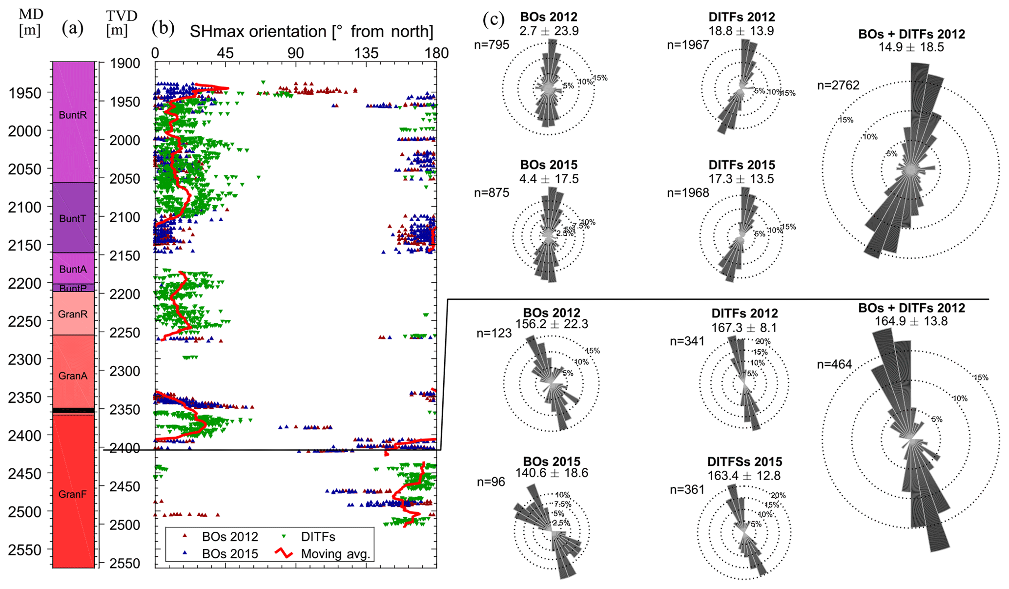
Figure 11 Evolution in the orientation of the maximum principal stress as a function of measured depth (MD) and vertical depth (TVD) in GRT-1 in 2012 and 2015. (a) Simplified lithologies along the GRT-1 borehole (see Fig. 8 for the legend). (b) Orientation of S_H from the azimuth of the maximum radial extension of the breakouts (BOs) from the datasets of 2012 (in blue) and 2015 (in red) acquired in GRT-1. In green is the orientation of S_H from the azimuth of drilling-induced tensile fractures (DITFs). The red line is a moving average of the orientation data. (c) Orientation in rose diagrams from the datasets displayed in panel (b).

Figure 2d, h and i show the orientation of breakouts (black dots) and DITFs (blue dots) measured in GRT-1. The measurements are compiled in Fig. 11 as circular histograms. We chose to only analyze data from the images acquired in 2012 and in 2015. Indeed, data acquired in 2013 were obtained without orientation, since the device was not functioning correctly, and are reoriented with respect to the 2012 data. Subsequently, the measurements carried out for the 2013 image do not bring additional constraints in terms of stress orientation.

In the Buntsandstein sediments, the failure orientation is stable and indicates that the principal stress S_H is oriented 15^∘ N ±19^∘ (one circular standard deviation). The same failure orientation persists in the upper section of the granite down to about 2270 m. Below this depth borehole failure orientation is much more variable as it seems to be influenced by the presence of major fault zones crossing the GRT-1 borehole at a depth of 2368 m (MD) (Vidal et al., 2016). Below 2420 m, which is the deepest large structure visible on the GRT-1 borehole image, the failure orientation indicates that S_H is oriented 165^∘ ±14^∘. This is significantly different from the orientation in the sediments with a 30^∘ counterclockwise rotation. Such differences in orientation with lithology have already been noted by Hehn et al. (2016) from an analysis of the orientation of drilling-induced fractures observed on borehole acoustic logs acquired in GRT-1. The orientation of S_H proposed by Hehn et al. (2016), i.e., globally N 155^∘ E in the basement and N 20^∘ E in the sedimentary layer, is consistent with our measurements.

Table 3 Mean density retained for each lithological layer and vertical depth (TVD) in each well.

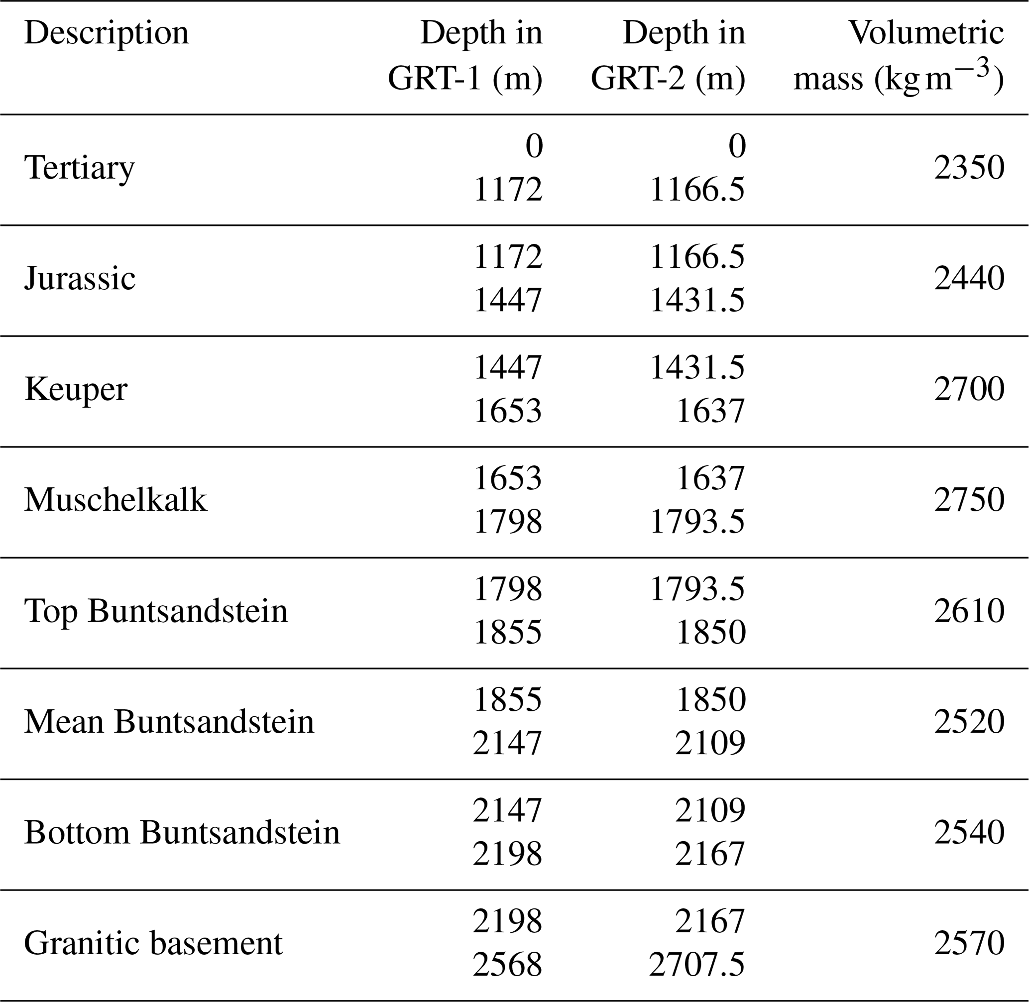
The geological study of the cuttings from the drilling of GRT-1 and GRT-2 enabled the determination of the rock density profile in both wells (Aichholzer et al., 2016). Thanks to this analysis, we estimate the mean density of each lithological layer. Table 3 shows the rock volumetric mass density as a function of the vertical depth (TVD). The magnitude of the vertical component S_v at depth is computed accordingly by integrating the volumetric mass density profile from the surface. A linear regression is fitted to the measurements obtained for the depth range studied here, i.e., 1900–2600 m. In the following, the vertical component S_v is computed from a linear trend expressed as a function of vertical depth (TVD) z:

$$\begin{array}{}\text{(6)}& S_{\mathrm{v}}\left[\mathrm{MPa}\right]=\mathrm{0.0248}\cdot z\left[\mathrm{m}\right]-\mathrm{0.83}.\end{array}$$

As the linear trend is expressed as a function of the vertical depth, we use the same equations in the computation steps leading to the S_H stress estimates in GRT-1 and GRT-2. As the density profile is integrated from surface to reservoir depth, the uncertainty on density adds up and the uncertainty on the vertical stress increases with depth consequently. Considering an uncertainty of 50 kg m⁻³ on the densities leads to a 2.5 MPa uncertainty on S_v at reservoir depth. This uncertainty is not significant compared to other uncertainties involved in the analysis, for example those related to the mechanical parameters chosen in the inversion of the maximum horizontal stress S_H.

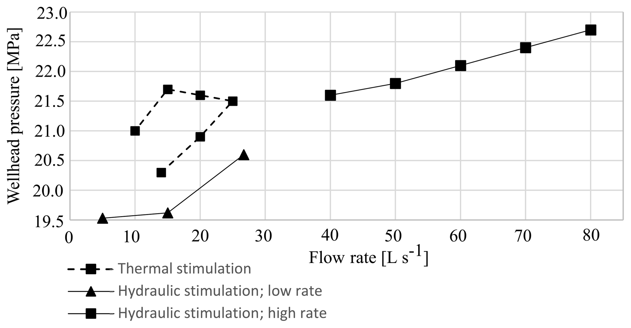
Figure 12 Stabilized wellhead pressure (MPa) as a function of flow rate (L s⁻¹) measured during the hydraulic stimulation of the GRT-1 well in 2013 (after Baujard et al., 2017).

8.2 Minimum horizontal stress S_h

We take the first-order assumption that the minimum horizontal stress S_h varies linearly with depth. Usually, the minimum horizontal stress S_h is estimated at depth from hydrofracture tests (i.e., Haimson and Cornet, 2003) but this was not done at the Rittershoffen site. As the data available for the ECOGI project do not enable us to compute a profile for the S_h stresses, our analysis of the minimum stress component is based on the numerous injection tests that were conducted in Soultz-sous-Forêts. We present in Fig. 12 the main trends computed from pressure-limiting behavior during hydraulic injections. For large depths, the injection tests performed in the deep wells (GPK-1, GPK-2, GPK-3 and/or EPS-1) of Soultz-sous-Forêts (Cornet et al., 2007; Valley and Evans, 2007b) give important constraints for the minimum horizontal stress S_h at the Rittershoffen site. In addition, the study of Rummel and Baumgartner (1991) provides estimates at shallow depth. In our analysis of the stress state in GRT-1 and GRT-2, we compute the horizontal minimum stress S_h as a function of the true vertical depth (TVD) z from the linear trend proposed by Cornet et al. (2007) for the site of Soultz-sous-Forêts (Fig. 15):

$$\begin{array}{}\text{(7)}& S_{\mathrm{h}}\left[\mathrm{MPa}\right]=\mathrm{0.015}\cdot z-\mathrm{7.3}.\end{array}$$

From the data available for the Rittershoffen site, i.e., the wellhead pressure measured during the hydraulic stimulation of GRT-1 (Baujard et al., 2017), we estimated a lower bound of the minimum horizontal stress S_h at 1913 m in Rittershoffen. The measurement enables us to verify the applicability of the linear trend inferred from acquisitions in Soultz-sous-Forêts to the Rittershoffen site. Figure 13 shows that the variation of wellhead pressure with the flow is slower during the high-rate hydraulic stimulation (above 40 L s⁻¹) than during the low-rate hydraulic stimulation (below 40 L s⁻¹). The change in behavior highlighted for higher values of the flow rate is interpreted as the beginning of a pressure capping resulting from fracture reactivation. Hydraulic stimulation operations aim at increasing pore pressure, which reduces the effective stress until pressure equals S_h in magnitude. In theory, an increase in pressure could activate new fractures, which results in the capping of the recorded pressure: in such a case, minimum horizontal stress is inferred at depth from the maximum pressure achieved during the hydraulic operations. Meanwhile, other processes (shearing of existing weak fractures, for example) could possibly result in the capping of pressure for lower pressure values.

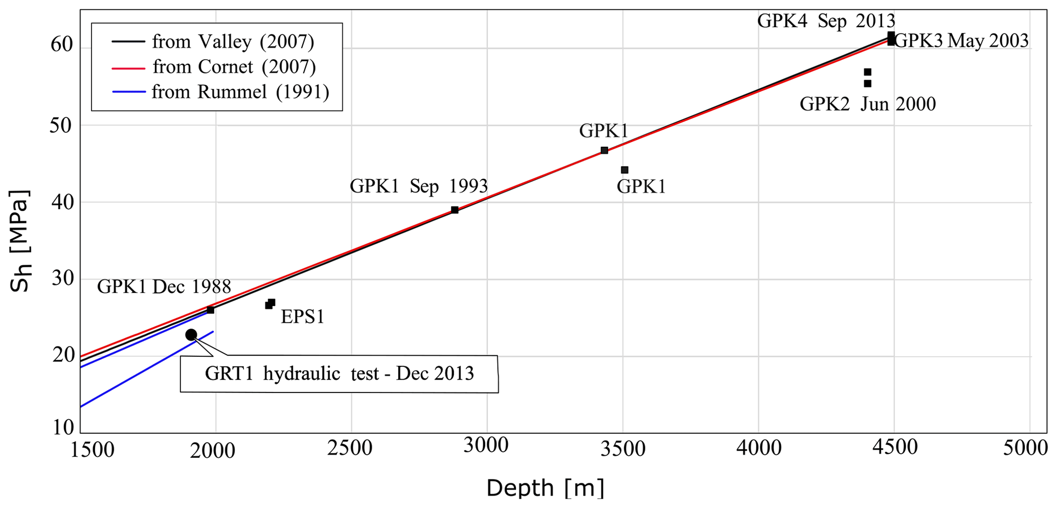
Figure 13 Minimal horizontal stress S_h (MPa) as a function of vertical depth (TVD) measured at the Soultz-sous-Forêts site from the analysis of high-volume injections in the GPK-1, GPK-2, GPK-3 and EPS-1 wells. The lower bound for the minimal horizontal stress S_h obtained from the analysis of the wellhead pressure measured during the stimulation of well GRT-1 in Rittershoffen is represented for comparison as a black circle.

The maximum pressure reached at 1913 m (TVD) during the hydraulic test is 22.6 MPa for a flow rate of 80 L s⁻¹ (Fig. 12). As the measurement is recorded at the end of a gradual but not definitive stabilization of the pressure with the flow rate, the 22.6 MPa stress measured at 1913 m consists of a lower bound for the minimum horizontal stress S_h at depth. It is compared to the Soultz-sous-Forêts trends in Fig. 13, and the measurement shows the consistency of the linear trend used in our analysis and inferred from the operations carried out at the Soultz-sous-Forêts site.

8.3 Thermal stresses

The cooling of the well imposed during drilling results in a thermal stress contribution. Accordingly, the characterization of the stress tensor necessitates the inclusion of a thermal stress analysis, which requires good knowledge of the thermal history of the well. We define the thermal contributions in the stress concentration at the borehole wall as σ^ΔTr, ${\mathit{\sigma }}_z^{\mathrm{\Delta }T}$ and ${\mathit{\sigma }}_{\mathit{\theta }}^{\mathrm{\Delta }T}$, which are respectively the radial, vertical and tangential components. The thermal stresses resulting from the temperature difference, Δt, between the borehole wall and the so-called ambient temperature, i.e., the initial temperature at that depth before the drilling phase or the temperature at a significant distance from the borehole (not influenced by the borehole perturbation), are expressed from Voight and Stephens (1982). These authors adapted the thermo-elastic solutions proposed by Ritchie and Sakakura (1956) for a hollow cylinder to study the stress concentrations at the borehole wall due to the application of a temperature difference. The radial component is null, and the tangential component is expressed as

$$\begin{array}{}\text{(8)}& {\mathit{\sigma }}_{\mathit{\theta }}^{\mathrm{\Delta }T}={\mathit{\sigma }}_z^{\mathrm{\Delta }T}=\mathit{\alpha }\cdot E\cdot {\displaystyle \frac{\mathrm{\Delta }T}{\left(\mathrm{1}-\mathit{\nu }\right)}},\end{array}$$

where α is the volumetric thermal expansion, E the Young modulus and ν the Poisson ratio. The volumetric thermal expansion, which is kept constant in the different layers crossed by the borehole, is $\mathit{\alpha }=\mathrm{14}\times {\mathrm{10}}^{-\mathrm{6}}$ K⁻¹. The Young modulus and Poisson ratio values applied at the different layers are indicated in Table 2. Figure 14 (green curve) presents the temperature log acquired in 2015 in GRT-1 (Baujard et al., 2017). It is plotted along with the temperature log acquired in 2013 (red curve). The comparison shows that temperature is close to be stable during that period in GRT-1. As a result, the temperature log acquired in 2015 in GRT-1 is used as an estimate of the ambient temperature since it is considered to be in equilibrium with the reservoir. Temperature at the borehole walls at drilling completion is best estimated from the temperature log acquired 4 d after drilling competition. The temperature log is presented in Fig. 14 (blue curve) as is the difference in temperature Δt computed from these logs. Interestingly, these temperature logs show a clear anomaly at 2360 m where the wells cross the main fault zone associated with a major permeable structure that controls two-thirds of the total flow during flow tests (Baujard et al., 2017).

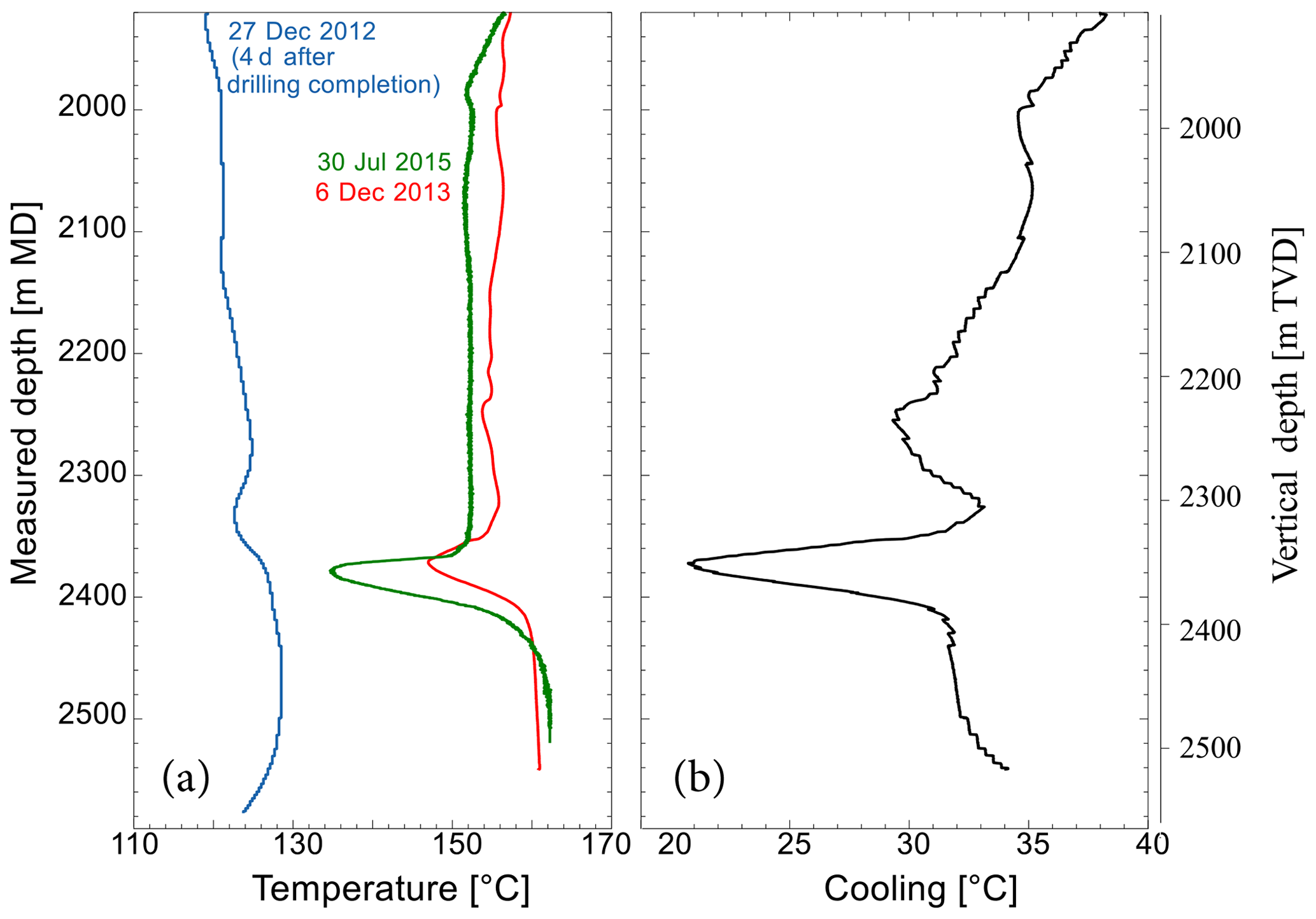
Figure 14 (a) Variation of temperature (^∘C) as a function of measured depth (MD) or vertical depth (TVD) estimated from the temperature log acquired in 2015 in GRT-1 (green curve), plotted along with the temperature log acquired in 2013 (red curve). The temperature log acquired 4 d after drilling completion (blue curve) enables us to estimate the temperature at the borehole wall during drilling. (b) Estimation of the difference between the wellbore temperature and the borehole wall temperature after completion Δt used in the evaluation of the thermal stress components.

8.4 Maximum horizontal stress S_H magnitude

The determination of the azimuthal position of the breakout edges and of their width from the analysis of the UBI images acquired in GRT-1 and GRT-2 enables us to estimate the maximum horizontal stress S_H, and to evaluate its evolution with depth and time. Here, we present the results of our inversion for multiple dates in GRT-1 and GRT-2.

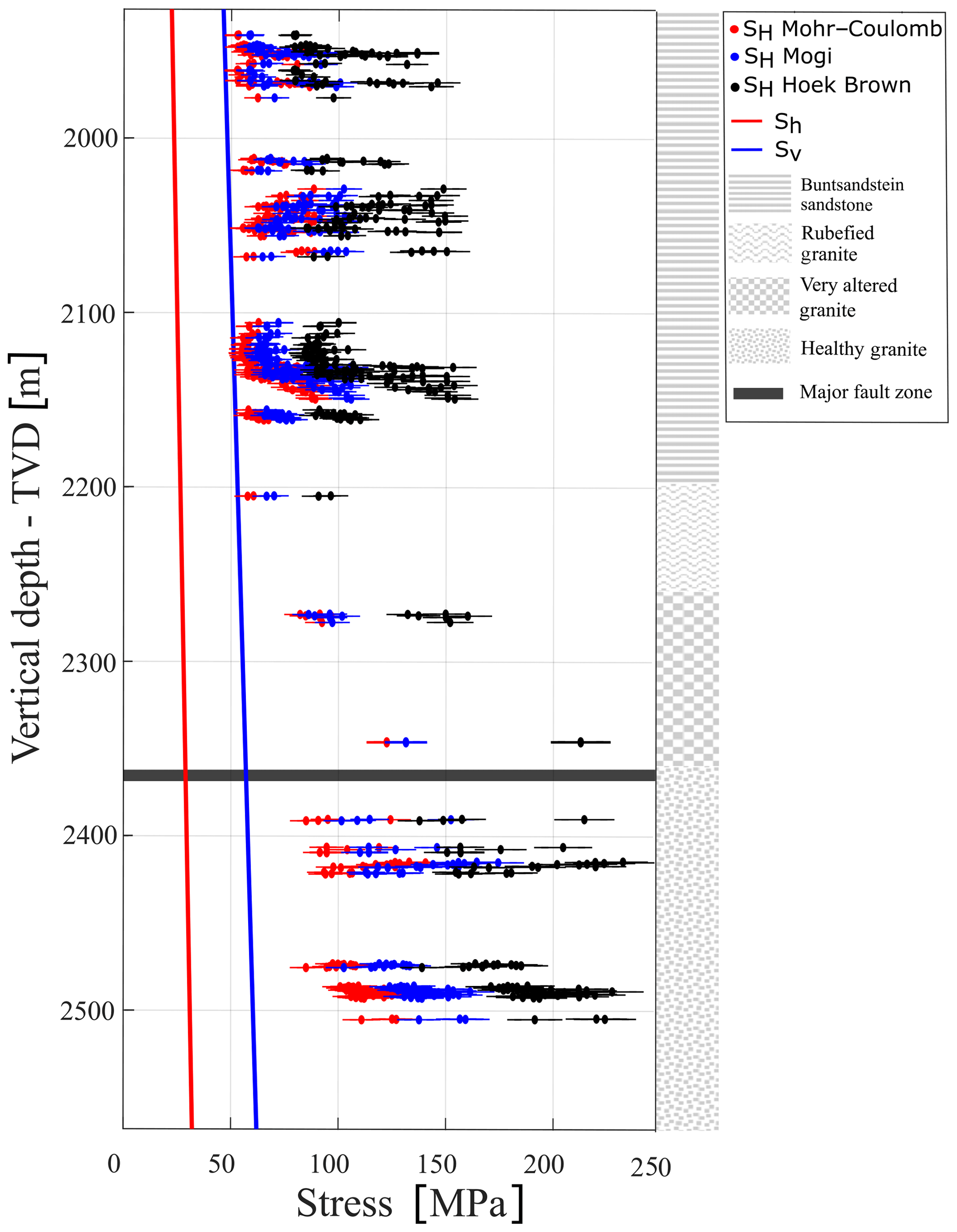
Figure 15 In situ stress state components S_h, S_v and S_H (MPa). Maximum horizontal stresses S_H are inverted with three distinctive failure criteria for the images acquired in 2013 in GRT-1. Error bars are calculated considering the error on the measurement of the breakout width, on the estimates of the elastic parameters, and on the S_h and S_v trends. The right column illustrates the four major lithological units retained in the model, and the horizontal band locates the major fault zone crossed by GRT-1.

In GRT-1, we obtain for each UBI log (in 2012, 2013 and 2015) three estimates of the magnitude of S_H, according to the failure criterion. Figure 15 shows estimates of the magnitude of S_H. The maximum horizontal stress S_H in GRT-1 is presented for the 2013 UBI log as a function of the true vertical depth (TVD), along with the S_h and S_v obtained previously (Eqs. 6 and 7). The horizontal error bars are calculated from the uncertainty on the elastic parameters, on the S_h and S_v estimates, and on the measurements of the width of the breakouts. The uncertainty ΔS_H is obtained by integration, taking into account the uncertainty Δx_i on each variable x_i involved in the estimation of S_H, i.e., the strength parameters, the S_h and S_v trends, and the width of the breakouts.

$$\begin{array}{}\text{(9)}& \mathrm{\Delta }f=\sum _i\left|{\displaystyle \frac{\partial f}{\partial x_i}}\right|\cdot \mathrm{\Delta }{x}_i\end{array}$$

Figure 15 shows that the S_H magnitudes vary significantly with the failure criterion. In particular, it shows that the S_H stresses computed using a criterion that considers the strengthening effect of the intermediate principal stress (i.e., in Mogi–Coulomb or Hoek–Brown) are higher than those calculated from a criterion that considers only the minimum and maximum principal stresses (i.e., in Mohr–Coulomb).

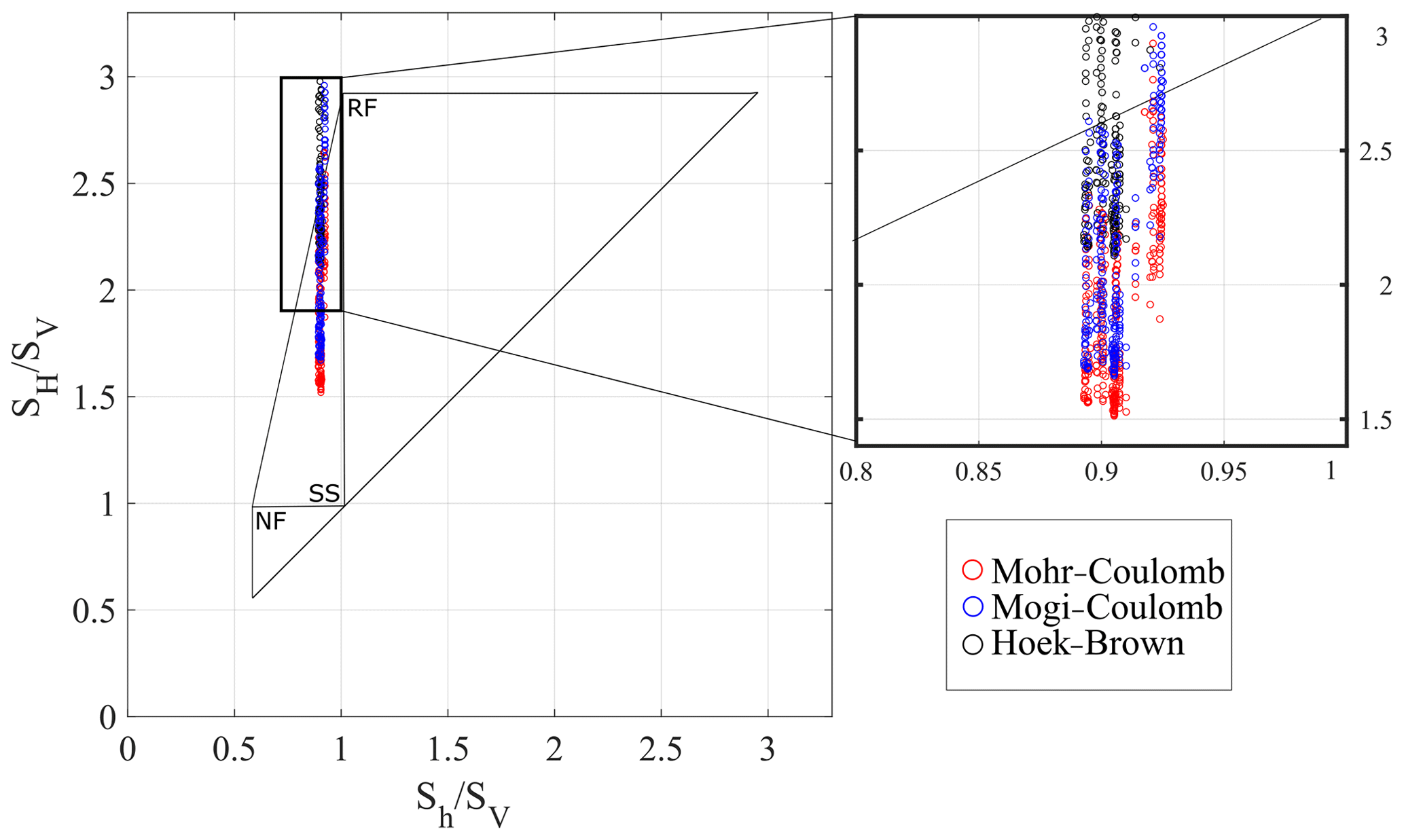
Figure 16 Normalized stress polygon defining stress states (S_H∕S_V, S_h∕S_V) at a depth of 2500 m in GRT-1, according to a Coulomb law with a coefficient of friction μ=1. The borders of the polygon correspond to an active fault situation. RF – reverse faulting, SS – strike-slip regime and NF – normal faulting refer to Anderson's faulting regimes. The plot includes stresses (S_H∕S_V–S_h∕S_V) calculated from the image of GRT-1 from 2013 for three different failure criteria (circles in color).

To choose the criterion that best describes the failure in the borehole, we use the approach proposed by Zoback et al. (2003) to display the stress state estimates presented in Fig. 15 in the stress polygon whose circumference is defined by a purely frictional, critically stressed Earth crust. For this purpose, we suppose that crustal strength is limited by a Coulomb friction criterion with a friction coefficient μ=1. We considered a depth of 2500 m to evaluate the vertical stress and assumed a hydrostatic pore pressure. The possible stress states from the 2013 UBI images are shown in Fig. 16 in a normalized S_H vs. S_h space. Because 2500 m is an upper boundary for the investigated depths in our study, the circumference of the polygon sets a maximum value for the maximum and minimum horizontal stresses S_H and S_h. The stresses are normalized by the vertical stress magnitude S_v to facilitate the comparison. The maximum principal stresses S_H measured using both our parameterized Hoek–Brown and Mogi–Coulomb criteria (blue and black dots) exceed the polygon boundaries. With our selection of parameters, the Mohr–Coulomb criterion was therefore retained as the most suitable for characterizing rock failure in our study. The same conclusion was drawn by Valley and Evans (2009) in Basel.

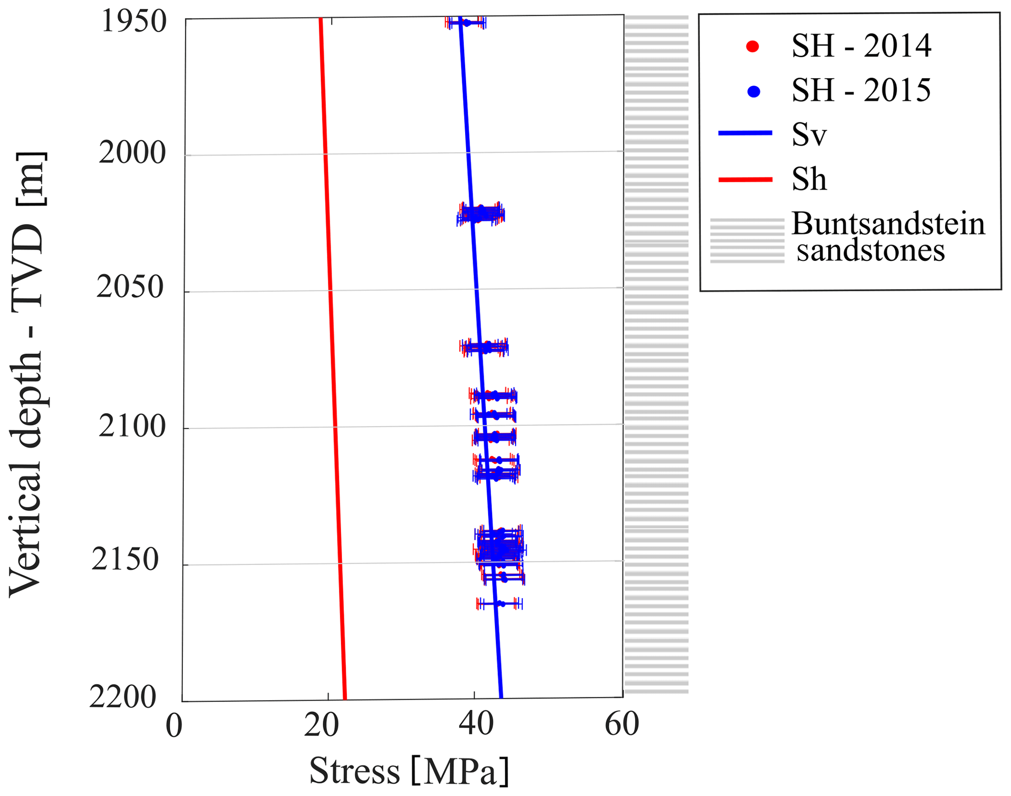
Figure 17 In situ stress components S_h, S_v and S_H (MPa) in the deviated well GRT-2. S_H stresses are inverted using a Mohr–Coulomb failure criterion and represented as a function of vertical depth (TVD) for the images acquired in 2014 and 2015. Error bars are calculated considering the errors on the measurements of the breakout widths, on the elastic parameters, and on the S_h and S_v trends. The right column illustrates the lithological unit retained in the model.

For GRT-2, we calculated the S_H magnitudes using only the Mohr–Coulomb criterion retained in the previous analysis. GRT-2 is highly deviated and the well was imaged in 2014 and 2015. The deviation is constant in the section of interest (i.e., the open hole): 37^∘ N, 355^∘ E. S_H stresses are shown as a function of vertical depth (TVD) in Fig. 17 with the corresponding error bars and plotted along with the S_h and S_v trends in GRT-2.

The impact of breakout widening on stress estimation can be evaluated from our time-lapse characterization of the stress tensor in GRT-1 and GRT-2. For GRT-2, Fig. 17 shows that S_H magnitude changes are limited between 2014 and 2015, given the uncertainty on the estimates. Figure 18 compares the S_H stresses estimated using the Mohr–Coulomb criterion on different dates in both the GRT-1 and GRT-2 wells. The systematic shift observed between the estimates in both wells suggests that the lower stresses estimated in the deviated well lead to a borehole wall stress concentration closer to the failure condition than in the vertical well. Figure 18 provides evidence of a time evolution of the S_H stress estimates in GRT-1. Panel (b) quantifies the differences in S_H stress between 2012 and 2015 in GRT-1 in a 1 MPa bins histogram. The confidence in the time evolution is discussed in the next section considering the error on S_H.

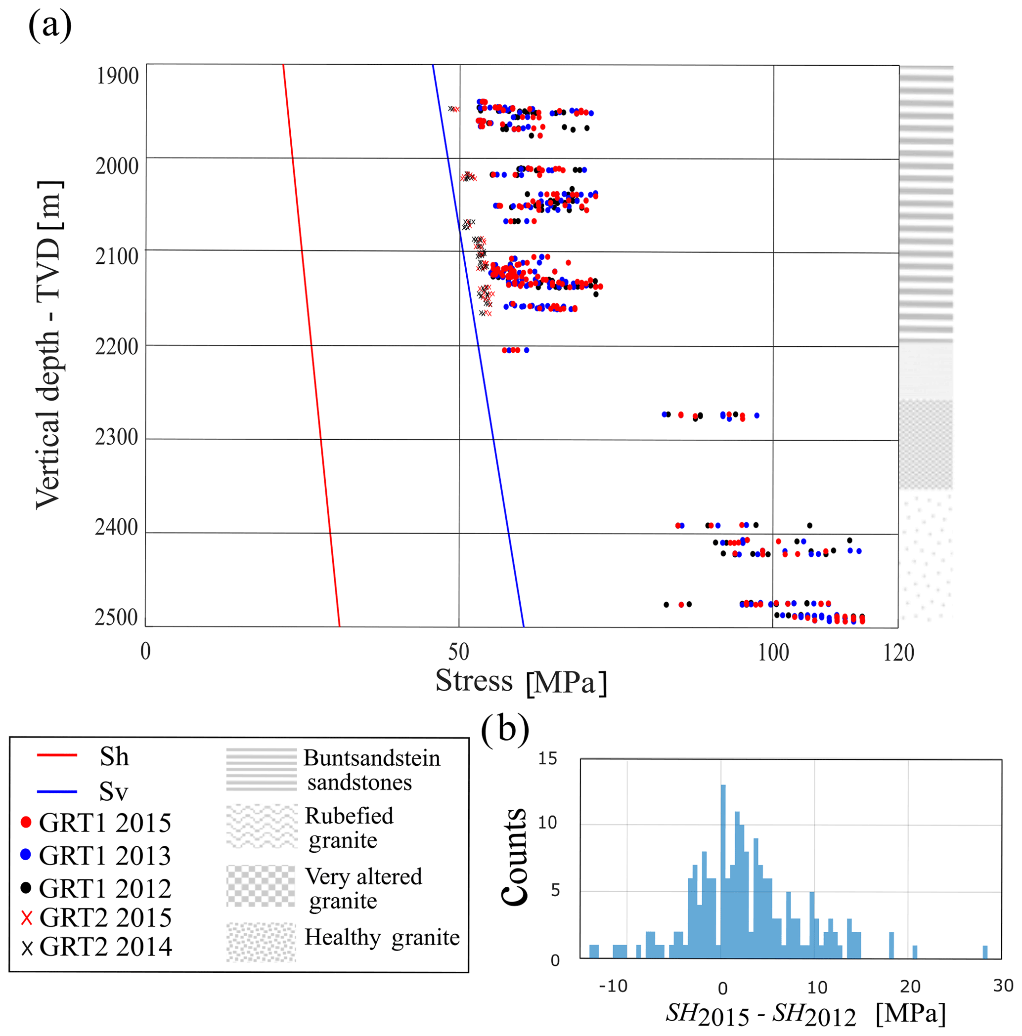
Figure 18 Panel (a) shows the in situ stress components S_h, S_v and S_H (MPa) in the deviated wells GRT-1 and GRT-2. S_H stresses (MPa) inverted with a Mohr–Coulomb criterion are obtained from an analysis of the images acquired in 2012–2013 and 2015 (black, blue and red circles, respectively) in GRT-1 and in 2014 and 2015 (black and red crosses, respectively) in GRT-2 as a function of vertical depth (TVD). The right column illustrates the four major lithological units retained in the model. Panel (b) is a histogram with 1 MPa bins representing the difference between the S_H stresses measured in GRT-1 in 2015 and in 2012.

9 Discussion

The dataset from the Rittershoffen geothermal project and our analyses allow us to discuss the evolution of the observed borehole failures both over time and with depth. The impact of these evolutions on our ability to estimate stress magnitude from borehole failure indicators is important.

9.1 Evolution of breakout geometry with time

Our analysis of the evolution of the breakout geometry with time proves a development of breakouts along well GRT-1 during the first year after drilling (Fig. 8). Indeed, we highlighted the fact that sections without breakouts in 2012, 4 d after drilling, present characteristic breakouts in 2013 and 2015, 1 year and 2.5 years after drilling, respectively. We also observe numerous length increases in the existing 2012 breakouts with time, in particular in the Buntsandstein. The difficulty is to link this evolution with time to a specific process: the time-dependant rheology of the rock (i.e., creep) or the effects of one of the stimulations (thermal, chemical or hydraulic). Moreover, the 2012 data were acquired at a period during which the thermal perturbations due to the drilling operations were still present. The data they are compared with were collected in 2013 or 2015 after hydraulic, thermal and chemical stimulations of the well. As a result, the observed changes could have taken place during the thermal equilibrium of the borehole after drilling or during the simulation operations, i.e., directly after drilling or later.

The conclusion from our time evolution analysis of the breakout geometry contradicts the usual assumption that breakouts deepen (i.e., an increase in the maximum radius measured in the borehole cross sections) but do not widen (i.e., an opening between the edges of the breakouts) with time (Zoback et al., 2003). However, the statistical approach applied in our study along the open hole of well GRT-1 must be interpreted with caution. Even if we propose a systematic analysis of a time-evolutive dataset, signal loss artifacts prevent an accurate measurement of borehole radius at some depths. This locally limits our ability to reliably estimate the depth of the breakout, i.e., the extension of the breakout in the radial direction. Given this limitation, we do not completely exclude the possibility that breakouts could have deepened with time. Our breakout width evaluation is also affected by uncertainty: deviation from the nominal cylindrical geometry of the borehole adds complexity to the measurements made considering the disputable positions of breakout edges. Meanwhile, we mitigated this difficulty by proposing a systematic analysis of all datasets to ensure a more consistent measurement and by attributing an uncertainty level to these values. Our study is thus more conclusive concerning this geometric parameter given that measured changes exceed our uncertainty level.

The widening observed in our dataset can be explained by the process of thermal stress dissipation. Indeed, the 30 to 35 ^∘C of cooling observed at the time of the 2012 logging is dissipated by the time of the 2013 logging (see Fig. 14). Assuming thermo-elastic properties of the material, the thermal hoop stresses implied by the cooling reach −17 to −20 MPa (Eq. 8). This will be sufficient to explain the change in breakout width without including additional time-dependent failure processes.

9.2 Evolution of breakout geometry with depth

The development of breakouts depends on the rock rheology and subsequently on the lithology. For our dataset, breakouts are more numerous and extended in the sedimentary cover than in the granitic basement (Fig. 2). Moreover, their development is more pronounced in the sedimentary cover when they develop with time vertically along the well (Fig. 8). Both observations are consistent with the fact that the sediments have on average a lower strength compared to the granitic rocks (Evans et al., 2009; Heap et al., 2019; Kushnir et al., 2018); i.e., conditions are closer to failure in the sediments.

Another important aspect of the variation of breakout geometry with depth is the evolution of their mean orientation. From the combined measure of the azimuth of the maximum radial extension of the breakouts (BOs) and the azimuth of drilling-induced tensile fractures (DITFs), we analyze in Fig. 11 the evolution with depth of the orientation of the maximum principal stress S_H. The measurements are repeated for the images acquired in GRT-1 in 2012 and in 2015. The consistency in orientation between our data and the 2012 and 2015 datasets (the 2013 dataset was not oriented) builds confidence in the reliability of these indicators.

Figure 11 suggests that the orientation measured in the granitic layers below 2420 m in Rittershoffen is consistent with the measurements carried out in the basement of Soultz-sous-Forêts (Valley and Evans, 2007b) and tends to reach regional orientation. The red line in Fig. 11 is a moving average of the orientation data. It is computed over a 20 m window in depth. The measurement is carried out only if 50 individual measurements or more are present in the averaging window. It shows that the orientation of the maximum principal stress S_H varies in the studied section. Another important aspect of Fig. 11 is the significant rotation of 30^∘ from NNW to NNE highlighted between the bottom and the top of our analyzed section. Such a rotation with depth has already been shown in the Upper Rhine Graben area in the Basel geothermal boreholes (Valley and Evans, 2009), in potash mines (Cornet and Röckel, 2012) and at the neighboring geothermal site of Soultz-sous-Forêts (Valley and Evans, 2007b). Hehn et al. (2016) have also provided evidence of local stress rotations in the sedimentary section of GRT-1 up to the upper Triassic (Keuper) from analyses of DITFs. The orientation measured here, which is above the limit set close to 2400 m MD (Fig. 11), is also consistent with the measurements of Hehn et al. (2016). They interpreted these variations to be related to mechanical contrasts between stiffer and softer rock layers. Another explanation for the stress rotation has been proposed by Cornet (2016). He suggested that the rotation is the result of the hydrostatic pressure effect on the effective friction angle in the Hoek–Brown failure criterion. In such a case, the rotation would be mainly a depth effect not linked to the presence of the Rittershoffen fault. The particularity of the measurements proposed in Fig. 11 is that the orientation of the maximum principal stress S_H deviates from the regional trend within the granitic basement, while the measurement in the upper basement aligns with the orientation of the sedimentary cover (Fig. 11). The presence of a major fault crossing the GRT-1 borehole at a depth of 2368 m MD (Vidal et al., 2016) could be the explanation for this rotation. The location of the observed stress rotation, i.e., in the basement and around 50 m above the major fault zone, does not assume that it is related to the stiffness contrast or decoupling between the sedimentary cover and the underlying basement, as typically assumed, but rather to the presence of a neighboring major fault zone. Considering a high-dipping fault geometry for this fault zone, it suggests that the geothermal well is tangent to the fault zone, explaining why breakouts are observed below but also above the major drain of the fault zone located at 2368 m (Fig. 11). Moreover, it was clearly demonstrated, based on continuous granite core analyses at Soultz, that the fault zone could have a significant thickness due to the presence of a damaged zone characterized by an intense hydrothermal alteration (Genter et al., 2010). Therefore, the absence of breakouts visible in the altered granitic section located just above the main fault drain and the anticipated rotation of the stress field at some distance in the hanging wall and the footwall of the fault zone confirm its major mechanical influence.

9.3 Evaluation of stress magnitude from breakout width

Our study shows the sensitivity of our approach toward the failure criterion chosen to describe the stability of the wellbore wall at a centimetric scale. The absence of consensus regarding the appropriate failure criterion to be used in the analysis of the borehole breakouts is a first limitation in our approach. Our analyses suggest that the Mogi–Coulomb and Hoek–Brown criteria tend to overestimate borehole wall strength because they lead to stress estimates that violate the frictional strength limit of the crust (Fig. 16), while the Mohr–Coulomb strength model leads to acceptable results. This conclusion is, however, dependent on the detailed parameterization of the failure criterion, which in Rittershoffen is supported by sparse data. The rock strength is among the main parameters that impact the stress magnitude assessment. Direct strength measurements are not available for the Rittershoffen project, since no cores were collected. We rely on measurements at the neighboring Soultz-sous-Forêts site where cores are available. However, even at Soultz-sous-Forêts, a systematic characterization of the rock strength of the various lithologies is not achievable, particularly for the sediments. Also, the mechanical and strength parameters are selected from an analysis of the core or cuttings performed at the laboratory scale. The measurements are thus not necessarily representative of the in situ conditions.

In addition to the uncertainty on the strength parameterization, the uncertainty on width determination and the evolution of width with time also impact the stress estimation. In the case of GRT-1, significant changes occur between the 2012 dataset (prior to reservoir stimulation operations) and the 2013–2015 datasets (after stimulation). Panel (b) of Fig. 18 shows that the changes in the S_H stresses between 2012 and 2015 in GRT-1 are larger than our measurement uncertainty for 15 % of the measurements and show principal stress increases. This change can be fully explained by the thermal equilibration of the well. The uncertainty on our data does not allow us to relate stress changes to the reservoir stimulation operations. Cornet (2016) showed that large-scale fluid injections conducted at the Soultz-sous-Forêts site generated large-scale failure zones whose orientation varies with depth. Based on the analyses of borehole failures, considerable stress orientation variations were also highlighted with depth at Rittershoffen (Hehn et al., 2016), at Soultz-sous-Forêts (Valley and Evans, 2007b) and at other sites (e.g., Valley and Evans, 2009; Cornet and Röckel, 2012). In this respect, our measurements at the Rittershoffen site confirm the conclusions drawn at many other sites regarding the change in stress orientation. However, given the difference in the fluid volumes injected into the wells of the two sites during the stimulation processes and in injection pressures, it is difficult to associate the rotation with depth with the hydraulic stimulation of GRT-1 and to apply the conclusions reached by Cornet (2016) in Soultz-sous-Forêts to the Rittershoffen site.

9.4 Stress magnitude evolution with depth

Stresses estimated in GRT-1 and GRT-2 suggest that S_H, in regards to the uncertainty, is generally close to the vertical principal stresses S_v, consistent with a transition between a strike-slip and a normal faulting regime (Anderson, 1951). This result is consistent with the stress characterization of the neighboring site of Soultz-sous-Forêts, where measurements have highlighted a normal faulting regime in the top granitic layers evolving into a strike-slip regime at greater depth. The uncertainty about our measurements and about the strength parameterization does not allow, however, for a decision on the faulting regime and its evolution with depth in Rittershoffen. A step in S_H magnitude is visible on our estimate in Fig. 18 at large depth (below 2250 m). This step occurs at the sediment–basement interface and could be explained by the effect of a stiffness contrast between lithologies (Corkum et al., 2018).

10 Conclusion

Thanks to the repeated UBI logging of geothermal wells GRT-1 and GRT-2 in Rittershoffen (France), this study focuses on the analysis of the evolution with time and depth of the borehole breakouts. The following conclusions are drawn.

1. There is clear evidence of the time evolution of the breakout, in particular in the sedimentary cover.

2. The evolution in time of the vertical length and the horizontal width of the breakouts is measured, benefiting from the development of a UBI image correlation technique. It is discussed in the limit of the estimated uncertainties. The vertical length of the breakouts is shown to increase with time. No variation in the depth of the breakouts in the radial direction was observed within the limit of the uncertainty of our analysis. However, width increases beyond the uncertainty of our determination were highlighted. This contradicts the common assumption that breakouts do not widen but only deepen until the borehole reaches a new stable state (Zoback et al., 2003).

3. The changes in breakout width occur between datasets collected prior to and after the reservoir stimulation that took place in 2013. However, the most likely effect on breakout width is the thermal equilibration of the wellbore, and our data do not provide evidence of stress changes resulting from reservoir stimulation.

In addition to this analysis, a study of the geometry of borehole failures in both wells leads us to propose a characterization of the in situ stress tensor at depth, including the orientation and magnitude of the three principal stresses. This detailed stress state analysis includes the estimation of thermal stresses. A Mohr–Coulomb criterion is retained here to estimate the principal stress magnitude as it is in our parameterization, which is the most consistent with a frictional strength limit in the crust. The strength parameterization is, however, uncertain due to the lack of mechanical testing on the Rittershoffen reservoir rocks. Given the uncertainties, we propose the following careful interpretation of our measurements.

1. Our analyses of the breakout geometry variation with depth suggest a change in mean orientation, with a 30^∘ rotation from NNW to NNE highlighted between the bottom and the top of our analyzed section. This observation is robust and independent of the strength parameterization. The rotation does not occur at the sediment–basement interface but is related to a high, steeply dipping major fault zone crossing the GRT-1 borehole at a depth of 2368 m (Vidal et al., 2016).

2. Our results also suggest a step in horizontal stress magnitude at the sediment to basement transition that would be consistent with a stiffness contrast between these two lithologies. However, such a step is determined by the choice of the failure criterion and its parameterization, which is uncertain at Rittershoffen.

3. S_H is generally slightly larger than the vertical principal stresses Sv consistently with a strike-slip to normal faulting transitional regime. This is consistent with stress characterization at the neighbor site of Soultz-sous-Forêts (Cornet et al., 2007; Klee and Rummel, 1993; Valley and Evans, 2007b)

The Rittershoffen borehole imaging dataset is unique in that repeated logging allowed for the study of the temporal evolution of borehole breakouts and the possible stress changes induced by reservoir stimulation. Our results change the common view that breakouts mostly deepen but do not widen. Further work is, however, required to reduce the uncertainties related to stress magnitude estimates from borehole breakouts and to quantify stress changes induced by reservoir stimulation.

Appendix A

The Kirsch equations are derived under 2-D plane conditions. They provide stress values in a case that is not suited to the one of real deviated boreholes, in which out-of-plane normal and shear stresses also exist. We consider two Cartesian coordinate frames: x–y–z having z aligned with the vertical and x^′–y^′–z^′, which is aligned with the three principal stresses denoted [${\mathit{\sigma }}_{x^{\prime }{x}^{\prime }}$, ${\mathit{\sigma }}_{y^{\prime }{y}^{\prime }}$, ${\mathit{\sigma }}_{z^{\prime }{z}^{\prime }}$]. We consider a long cylindrical cavity of radius a. Its axis is arbitrarily oriented with respect to the principal stress state in the Earth. The borehole axis tilts at an angle ϕ relative to the x axis. The third cylindrical r–θ–ζ coordinate frame is borehole centric with the ζ axis, which is coincident with the borehole axis. The azimuth with respect to the borehole axis is denoted θ.

The borehole centric stresses are expressed as a function of the direction of cosines aij, enabling us to transform the principal axes x^′–y^′–z^′ to the x–y–z frame according to Eq. (A1),

$$\begin{array}{}\text{(A1)}& {\mathit{\sigma }}^{\prime }={\mathbf{A}}^{.}{\mathit{\sigma }}^{.}{\mathbf{A}}^{\mathrm{T}},\end{array}$$

where the rotation matrix A is composed of the direction cosines aij:

$$\mathbf{A}=\left[\begin{array}{lll}ax{x}^{\prime }& ax{y}^{\prime }& ax{z}^{\prime }\\ a{y}^{\prime }{x}^{\prime }& ay{y}^{\prime }& ay{z}^{\prime }\\ a{z}^{\prime }x& a{z}^{\prime }y& az{z}^{\prime }\end{array}\right].$$

Equations (A2)–(A7) express the borehole-centric stresses as a function of directional coefficients α₁, α₂, α₃, γ₁ and γ₂. They include the contribution of fluid pressure P_f. Indeed, the pressure of the fluid in the mud column increases with depth, which produces tensile hoop stress and compressive radial stress. Equations (A2)–(A7) also include the time-dependant contribution due to temperature changes. The thermal stresses ${\mathit{\sigma }}_{\mathit{\theta }}^{\mathrm{\Delta }T}$ and ${\mathit{\sigma }}_r^{\mathrm{\Delta }T}$, resulting from the temperature difference, Δt, between the temperature applied at the borehole wall and the initial temperature at that depth before perturbation or the temperature at a significant distance from the borehole (not influenced by the borehole perturbation), are expressed from Voight and Stephens (1982). The radial component is null, and the tangential component expressed in Eq. (8) shows that an increase in temperature at r=a effects the compressive hoop stress.

$$\begin{array}{}\text{(A2)}& {\displaystyle }{\mathit{\sigma }}_{rr}=P_{\mathrm{f}}+{\mathit{\sigma }}_r^{\mathrm{\Delta }T}\text{(A3)}& {\displaystyle }{\mathit{\sigma }}_{\mathit{\theta }\mathit{\theta }}=\mathrm{2}{\mathit{\alpha }}_{\mathrm{1}}-\mathrm{4}{\mathit{\alpha }}_{\mathrm{2}}\cos \mathrm{2}\mathit{\theta }-\mathrm{4}{\mathit{\alpha }}_{\mathrm{3}}\sin \mathrm{2}\mathit{\theta }-P_{\mathrm{f}}+{\mathit{\sigma }}_{\mathit{\theta }}^{\mathrm{\Delta }T}\text{(A4)}& {\displaystyle }{\mathit{\sigma }}_{\mathit{\zeta }\mathit{\zeta }}=\mathit{\beta }\mathrm{1}-\mathrm{4}\mathit{\nu }({\mathit{\alpha }}_{\mathrm{2}}\cos \mathrm{2}\mathit{\theta }+{\mathit{\alpha }}_{\mathrm{3}}\sin \mathrm{2}\mathit{\theta })\text{(A5)}& {\displaystyle }{\mathit{\tau }}_{\mathit{\theta }\mathit{\zeta }}=\mathrm{2}{\mathit{\gamma }}_{\mathrm{1}}\cos \mathit{\theta }+\mathrm{2}{\mathit{\gamma }}_{\mathrm{2}}\sin \mathit{\theta }\text{(A6)}& {\displaystyle }{\mathit{\tau }}_{r\mathit{\zeta }}=\mathrm{0}\text{(A7)}& {\displaystyle }{\mathit{\tau }}_{\mathit{\theta }r}=\mathrm{0}\end{array}$$

The geometrical coefficients involved in Eqs. (A2)–(A7) are expressed as a function of the three far-field principal stress states [${\mathit{\sigma }}_{x^{\prime }{x}^{\prime }}$, ${\mathit{\sigma }}_{y^{\prime }{y}^{\prime }}$, ${\mathit{\sigma }}_{z^{\prime }{z}^{\prime }}$] and as a function of the geometrical rotations aij.

$$\begin{array}{}\text{(A8)}& {\displaystyle }\begin{array}{rl}{\mathit{\alpha }}_{\mathrm{1}}& ={\displaystyle \frac{\mathrm{1}}{\mathrm{2}}}\left[\right(a_{x^{\prime }x}^{\mathrm{2}}{\sin }^{\mathrm{2}}\mathrm{\Phi }+a_{x^{\prime }y}^{\mathrm{2}}+a_{x^{\prime }z}^{\mathrm{2}}{\cos }^{\mathrm{2}}\mathrm{\Phi }\\ & -\mathrm{2}{a}_{x^{\prime }z}^{\mathrm{2}}{a}_{x^{\prime }x}^{\mathrm{2}}\sin \mathrm{\Phi }\cos \mathrm{\Phi }){\mathit{\sigma }}_{x^{\prime }{x}^{\prime }}\\ & +(a_{y^{\prime }x}^{\mathrm{2}}{\sin }^{\mathrm{2}}\mathrm{\Phi }+a_{y^{\prime }y}^{\mathrm{2}}+a_{y^{\prime }z}^{\mathrm{2}}{\cos }^{\mathrm{2}}\mathrm{\Phi }\\ & -\mathrm{2}{a}_{y^{\prime }z}^{\mathrm{2}}{a}_{y^{\prime }x}^{\mathrm{2}}\sin \mathrm{\Phi }\cos \mathrm{\Phi })\\ & {\mathit{\sigma }}_{y^{\prime }{y}^{\prime }}+(a_{z^{\prime }x}^{\mathrm{2}}{\sin }^{\mathrm{2}}\mathrm{\Phi }+a_{z^{\prime }y}^{\mathrm{2}}+a_{z^{\prime }z}^{\mathrm{2}}{\cos }^{\mathrm{2}}\mathrm{\Phi }\\ & -\mathrm{2}{a}_{z^{\prime }z}^{\mathrm{2}}{a}_{z^{\prime }x}^{\mathrm{2}}\sin \mathrm{\Phi }\cos \mathrm{\Phi }\left){\mathit{\sigma }}_{z^{\prime }{z}^{\prime }}\right]\end{array}\text{(A9)}& {\displaystyle }\begin{array}{rl}{\mathit{\alpha }}_{\mathrm{2}}& ={\displaystyle \frac{\mathrm{1}}{\mathrm{2}}}\left[\right(-a_{x^{\prime }x}^{\mathrm{2}}{\sin }^{\mathrm{2}}\mathrm{\Phi }+a_{x^{\prime }y}^{\mathrm{2}}-a_{x^{\prime }z}^{\mathrm{2}}{\cos }^{\mathrm{2}}\mathrm{\Phi }\\ & +\mathrm{2}{a}_{x^{\prime }z}^{\mathrm{2}}{a}_{x^{\prime }x}^{\mathrm{2}}\sin \mathrm{\Phi }\cos \mathrm{\Phi }){\mathit{\sigma }}_{x^{\prime }{x}^{\prime }}+(-a_{y^{\prime }x}^{\mathrm{2}}{\sin }^{\mathrm{2}}\mathrm{\Phi }+a_{y^{\prime }y}^{\mathrm{2}}\\ & -a_{y^{\prime }z}^{\mathrm{2}}{\cos }^{\mathrm{2}}\mathrm{\Phi }+\mathrm{2}{a}_{y^{\prime }z}^{\mathrm{2}}{a}_{y^{\prime }x}^{\mathrm{2}}\sin \mathrm{\Phi }\cos \mathrm{\Phi }){\mathit{\sigma }}_{y^{\prime }{y}^{\prime }}\\ & +(-a_{z^{\prime }x}^{\mathrm{2}}{\sin }^{\mathrm{2}}\mathrm{\Phi }+a_{z^{\prime }y}^{\mathrm{2}}-a_{z^{\prime }z}^{\mathrm{2}}{\cos }^{\mathrm{2}}\mathrm{\Phi }\\ & +\mathrm{2}{a}_{z^{\prime }z}^{\mathrm{2}}{a}_{z^{\prime }x}^{\mathrm{2}}\sin \mathrm{\Phi }\cos \mathrm{\Phi }\left){\mathit{\sigma }}_{z^{\prime }{z}^{\prime }}\right]\end{array}\text{(A10)}& {\displaystyle }\begin{array}{rl}{\mathit{\alpha }}_{\mathrm{3}}& =(a_{x^{\prime }y}{a}_{x^{\prime }z}\cos \mathrm{\Phi }-a_{x^{\prime }x}{a}_{x^{\prime }y}\sin \mathrm{\Phi }){\mathit{\sigma }}_{x^{\prime }{x}^{\prime }}\\ & +(a_{y^{\prime }y}{a}_{y^{\prime }z}\cos \mathrm{\Phi }-a_{y^{\prime }x}{a}_{y^{\prime }y}\sin \mathrm{\Phi }){\mathit{\sigma }}_{y^{\prime }{y}^{\prime }}\\ & +(a_{z^{\prime }y}{a}_{z^{\prime }z}\cos \mathrm{\Phi }-a_{z^{\prime }x}{a}_{z^{\prime }y}\sin \mathrm{\Phi }){\mathit{\sigma }}_{z^{\prime }{z}^{\prime }}\end{array}\text{(A11)}& {\displaystyle }\begin{array}{rl}{\mathit{\gamma }}_{\mathrm{1}}& =[-a_{x^{\prime }x}^{\mathrm{2}}\sin \mathrm{\Phi }\cos \mathrm{\Phi }+a_{x^{\prime }z}^{\mathrm{2}}\cos \mathrm{\Phi }\sin \mathrm{\Phi }\\ & +a_{x^{\prime }z}{a}_{x^{\prime }x}({\cos }^{\mathrm{2}}\mathrm{\Phi }-{\sin }^{\mathrm{2}}\mathrm{\Phi })]{\mathit{\sigma }}_{x^{\prime }{x}^{\prime }}\\ & +[-a_{y^{\prime }x}^{\mathrm{2}}\sin \mathrm{\Phi }\cos \mathrm{\Phi }\\ & +a_{y^{\prime }z}^{\mathrm{2}}\cos \mathrm{\Phi }\sin \mathrm{\Phi }+a_{y^{\prime }z}{a}_{y^{\prime }x}({\cos }^{\mathrm{2}}\mathrm{\Phi }-{\sin }^{\mathrm{2}}\mathrm{\Phi })]{\mathit{\sigma }}_{y^{\prime }{y}^{\prime }}\\ & +[-a_{z^{\prime }x}^{\mathrm{2}}\sin \mathrm{\Phi }\cos \mathrm{\Phi }+a_{z^{\prime }z}^{\mathrm{2}}\cos \mathrm{\Phi }\sin \mathrm{\Phi }\\ & +a_{z^{\prime }z}{a}_{z^{\prime }x}({\cos }^{\mathrm{2}}\mathrm{\Phi }-{\sin }^{\mathrm{2}}\mathrm{\Phi })\left]{\mathit{\sigma }}_{z^{\prime }{z}^{\prime }}\right]\end{array}\text{(A12)}& {\displaystyle }\begin{array}{rl}{\mathit{\gamma }}_{\mathrm{2}}& =(-a_{x^{\prime }y}{a}_{x^{\prime }z}\sin \mathrm{\Phi }-a_{x^{\prime }x}{a}_{x^{\prime }y}\cos \mathrm{\Phi }){\mathit{\sigma }}_{x^{\prime }{x}^{\prime }}\\ & +(-a_{y^{\prime }y}{a}_{y^{\prime }z}\sin \mathrm{\Phi }-a_{y^{\prime }x}{a}_{y^{\prime }y}\cos \mathrm{\Phi }){\mathit{\sigma }}_{y^{\prime }{y}^{\prime }}\\ & +(-a_{z^{\prime }y}{a}_{z^{\prime }z}\sin \mathrm{\Phi }-a_{z^{\prime }x}{a}_{z^{\prime }y}\cos \mathrm{\Phi }){\mathit{\sigma }}_{z^{\prime }{z}^{\prime }}\end{array}\end{array}$$