the Creative Commons Attribution 4.0 License.
the Creative Commons Attribution 4.0 License.
 | 25 Jun 2020
Combined numerical and experimental study of microstructure and permeability in porous granular media
Philipp Eichheimer
Marcel Thielmann
Wakana Fujita
Gregor J. Golabek
Michihiko Nakamura
Satoshi Okumura
Takayuki Nakatani
Maximilian O. Kottwitz
Fluid flow on different scales is of interest for several Earth science disciplines like petrophysics, hydrogeology and volcanology. To parameterize fluid flow in large-scale numerical simulations (e.g. groundwater and volcanic systems), flow properties on the microscale need to be considered. For this purpose experimental and numerical investigations of flow through porous media over a wide range of porosities are necessary. In the present study we sinter glass bead media with various porosities and measure the permeability experimentally. The microstructure, namely effective porosity and effective specific surface, is investigated using image processing. We determine flow properties like tortuosity and permeability using numerical simulations. We test different parameterizations for isotropic low-porosity media on their potential to predict permeability by comparing their estimations to computed and experimentally measured values.
- Article
(2274 KB) - Full-text XML
-
Supplement
(187 KB) - BibTeX
- EndNote


An understanding of the transport and storage of geological fluids in sediments, crust and mantle is of major importance for several Earth science disciplines including volcanology, hydrology and petroleum geoscience (e.g. Manwart et al., 2002; Ramandi et al., 2017; Honarpour, 2018). In volcanic settings melt segregation from partially molten rocks controls the magma chemistry, and outgassing of magmas influences both magma ascent and eruption explosivity (Collinson and Neuberg, 2012; Lamur et al., 2017; Mueller et al., 2005). In hydrogeology fluid flow affects groundwater exploitation and protection (Domenico and Schwartz, 1998; Hölting and Coldewey, 2019), whereas in petroleum geoscience it controls oil recovery efficiency (Suleimanov et al., 2011; Hendraningrat et al., 2013; Zhang et al., 2014).
A key parameter for fluid flow is permeability. Permeability estimations have been performed on several scales ranging from the pore scale (Brace, 1980) to the macroscale (Fehn and Cathles, 1979; Norton and Taylor Jr, 1979; Gleeson and Ingebritsen, 2016). As permeability on the macroscale is a function of its microstructure it is necessary to accurately predict permeability based on microscale properties (Mostaghimi et al., 2013). To achieve this goal, various experimental and numerical approaches have been developed over the years (e.g. Keehm, 2003; Andrä et al., 2013a; Gerke et al., 2018; Saxena et al., 2017).
Assuming laminar flow (Bear, 1988; Matyka et al., 2008), flow through porous media can be described using Darcy's law (Darcy, 1856), which relates the fluid flux Q to an applied pressure difference ΔP:
where k is the permeability, A is the cross-sectional area, η is the fluid viscosity and L is the length of the domain.
Accurately determining and predicting permeability is thus of crucial importance to quantify fluid fluxes in porous media. Until today it remains challenging to relate permeability to the microstructure of porous media. This has resulted in numerous parameterizations developed for different materials and structures (Kozeny, 1927; Carman, 1937, 1956; Martys et al., 1994; Revil and Cathles, 1999; Garcia et al., 2009).
A first simple capillary model to predict the permeability of a porous medium was proposed by Kozeny (1927):
where k0 is the dimensionless Kozeny constant depending on the channel geometry (e.g. k0=0.5 for cylindrical capillaries), ϕ is the porosity and S is the specific surface area (ratio of exposed surface area to bulk volume). Later this relation was extended by Carman (1937, 1956) to predict fluid flow through a granular bed with a given microstructure. To account for the effect of the microstructure on fluid flow, Carman (1937, 1956) introduced the term tortuosity, which he defined as the ratio of effective flow path Le to a straight path L.
Introducing this relation into Eq. (2) leads to the well-known Kozeny–Carman equation:
Using experimental data, Carman (1956) determined that tortuosity τ is . Today, the Kozeny–Carman equation – or variants thereof – is widely used in volcanology (Klug and Cashman, 1996; Mueller et al., 2005; Miller et al., 2014), hydrogeology (Wang et al., 2017; Taheri et al., 2017), two-phase and multi-phase flow studies (Wu et al., 2012; Keller and Katz, 2016; Keller and Suckale, 2019), and soil sciences (Chapuis and Aubertin, 2003; Ren et al., 2016). The Kozeny–Carman equation was derived assuming that the medium consists only of continuous curved channels with a constant cross section (Carman, 1937; Bear, 1988). However, in porous media pathways most likely do not obey these assumptions. Applying this equation to porous media therefore remains challenging and in some cases fails for low porosities (Bernabe et al., 1982; Bourbie et al., 1992) or mixtures of different shapes and material sizes (Carman, 1937; Wyllie and Gregory, 1955). Consequently, alternative permeability parameterizations have been developed by different authors (Martys et al., 1994; Revil and Cathles, 1999; Garcia et al., 2009).
Using numerical modelling, Martys et al. (1994) derived a universal scaling law for various overlapping and non-overlapping sphere packings, which reads as
with f=4.2 and ϕc being the critical porosity, below which no connected pore space exists. They showed that Eq. (5) is valid for a variety of porous media including mono-sized sphere packings, glass bead samples and experimentally measured sandstones. Despite the predictive power of this parameterization it might not give reasonable estimations for permeability in the case that the porous medium consists of rough surfaces and large isolated regions (voids).
The study of Revil and Cathles (1999) used electrical parameters to derive the permeability of different types of shaly sands, i.e. the permeability of a clay-free sand and the permeability of a pure shale. By using electrical parameters which separate pore throat from total porosity and effective from total hydraulic radius, Revil and Cathles (1999) were able to improve the Kozeny–Carman relation, being only dependent on grain size. In a first step the authors developed a model for the permeability of a clay-free sand as a function of the grain diameter, the porosity and the electrical cementation exponent reading as
with Λ being the effective electrical pore radius, R being the grain radius, m being the cementation exponent and F being the formation factor. Using the relation of the formation factor to porosity by Archie's law (Waxman and Smits, 1968), m=1.8 (Waxman and Smits, 1968) and d=2R for the grain diameter, the authors derived a permeability parameterization for natural sandstones:
which is in good agreement with experimentally measured data by Berg (1975).
Based on numerical simulations of fluid flow in polydisperse grain packings with irregular shapes, Garcia et al. (2009) proposed an alternative parameterization by fitting the numerical results with the following equation:
where D2 is the squared harmonic mean diameter of the grains. They also showed that this parameterization fits the experimental results quite well and concluded that grain shape and size polydispersity have a small but noticeable effect on permeability.
As can been seen from Eqs. (4), (5), (7) and (8) the different parameterizations focus on specific types of porous media and relate different microstructural properties to permeability. While properties such as porosity and mean grain diameter are relatively straightforward to determine, others, such as specific surface and tortuosity, are much harder to access. This is why several parameterizations have been developed to quantify these properties (Comiti and Renaud, 1989; Pech, 1984; Mota et al., 2001; Pape et al., 2005). These studies either use experimental, analytical or numerical approaches for mostly two-dimensional porous media with porosities >30 %.
Since the ascent of digital rock physics (DRP), it has become viable to study the microstructures of porous media in more detail using micro-computed tomography (micro-CT) and nuclear magnetic resonance (NMR) images (Arns et al., 2001; Arns, 2004; Dvorkin et al., 2011). Together with numerical models, these images can then be used to compute fluid flow within porous media to determine their permeability. For this purpose several numerical methods, including the finite-element (FEM), finite-difference (FDM) and lattice Boltzmann method (LBM) (Saxena et al., 2017; Andrä et al., 2013a; Gerke et al., 2018; Shabro et al., 2014; Manwart et al., 2002; Bird et al., 2014), have been used.
Yet, very few data sets exist that systematically investigate microstructure (porosity and specific surface) and related flow parameters (tortuosity and permeability), in particular at porosities <30 %. Most previous studies either measure permeability experimentally without investigating its microstructure or compute permeability and related microstructural parameters that cannot be compared to experimental data sets. To remedy this issue, we sinter porous glass bead samples with porosities ranging from 1.5 % to 21 % and investigate their microstructure using image processing. This porosity range is representative of sedimentary rocks up to a depth of ≈20 km (Bekins and Dreiss, 1992). Permeability is then measured experimentally using a permeameter (see Sect. 2.2; Takeuchi et al., 2008; Okumura et al., 2009) and numerically using the finite-difference code LaMEM (see Sect. 2.7; Kaus et al., 2016; Eichheimer et al., 2019a). The theoretical permeability predictions described above in Eqs. (4), (5), (7) and (8) require microstructural input parameters such as porosity, specific surface and tortuosity. Within this study these parameters are determined and related to porosity. We therefore provide permeability parameterizations depending on porosity only and verify against numerically and experimentally determined values.
Here we first describe the experimental workflow including sample sintering and permeability measurement, followed by the numerical workflow featuring image processing, the computation of fluid velocities, and the determination of both tortuosity and permeability. Figure 1 shows an overview of the entire workflow, which will be explained in detail in the following section.
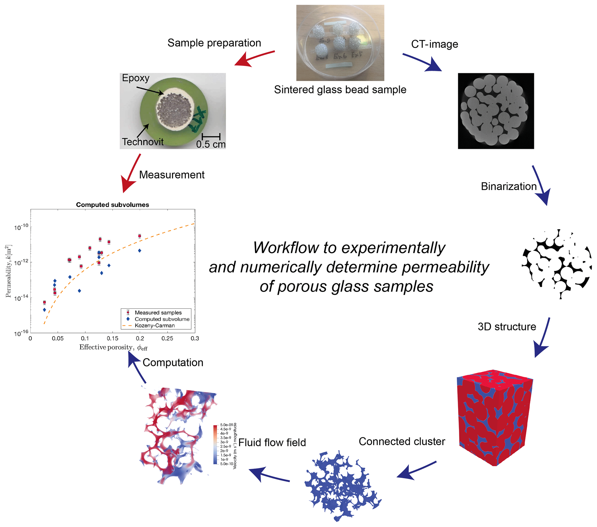
Figure 1Workflow process map – red arrows mark the experimental workflow, whereas blue arrows indicate the numerical workflow.
2.1 Sample sintering
Glass bead cylinders with different porosities were sintered under experimental conditions as summarized in Table 1. For this purpose soda–lime glass beads with diameters ranging from 0.9 to 1.4 mm were utilized as starting material (see grain size distribution in Appendix D). For each sample, we prepared a graphite cylinder with an 8.0 mm inner diameter and an approximately 10 mm height. Additional samples with diameters of 10 and 14 mm were prepared to check for size effects (see Table 1a). At the bottom of the graphite cylinder a graphite disc (11.5 mm diameter and 3.0 mm thick) was attached using a cyanoacrylate adhesive (see Fig. 2 inset). The glass beads were poured into the graphite cylinder and compressed with steel rods (8–14 mm diameter) before heating.
The glass bead samples were then sintered in a muffle furnace at 710 ∘C under atmospheric pressure. The temperature of 710 ∘C was found to be suitable for sintering the glass beads as it is slightly below the softening temperature of soda–lime glass at around 720–730 ∘C (Napolitano and Hawkins, 1964) and well above the glass transition temperature of soda–lime glass at ≈550 ∘C (Wadsworth et al., 2014). At 710 ∘C the viscosity of the employed soda–lime glass is on the order of 107 Pa s (Kuczynski, 1949; Napolitano and Hawkins, 1964; Wadsworth et al., 2014), allowing for viscous flow of the glass beads at their contact surface driven by surface tension. Using different time spans ranging 60–600 min the viscous flow at 710 ∘C controls the resulting porosity of the sample.After sintering, the sample was cooled down to 550–600 ∘C within ≈5 min. Afterwards the sample was taken out of the furnace to adjust to room temperature and prevent thermal cracking of the sample. In a next step the graphite container was removed from the sample. It should be noted that during the process of sintering gravity slightly affects the porosity distribution within the glass bead sample (see Fig. 2). However, the subsamples used to compute the numerical permeability do not cover the whole height of the sample; thus, the effect of compaction on the results is limited.
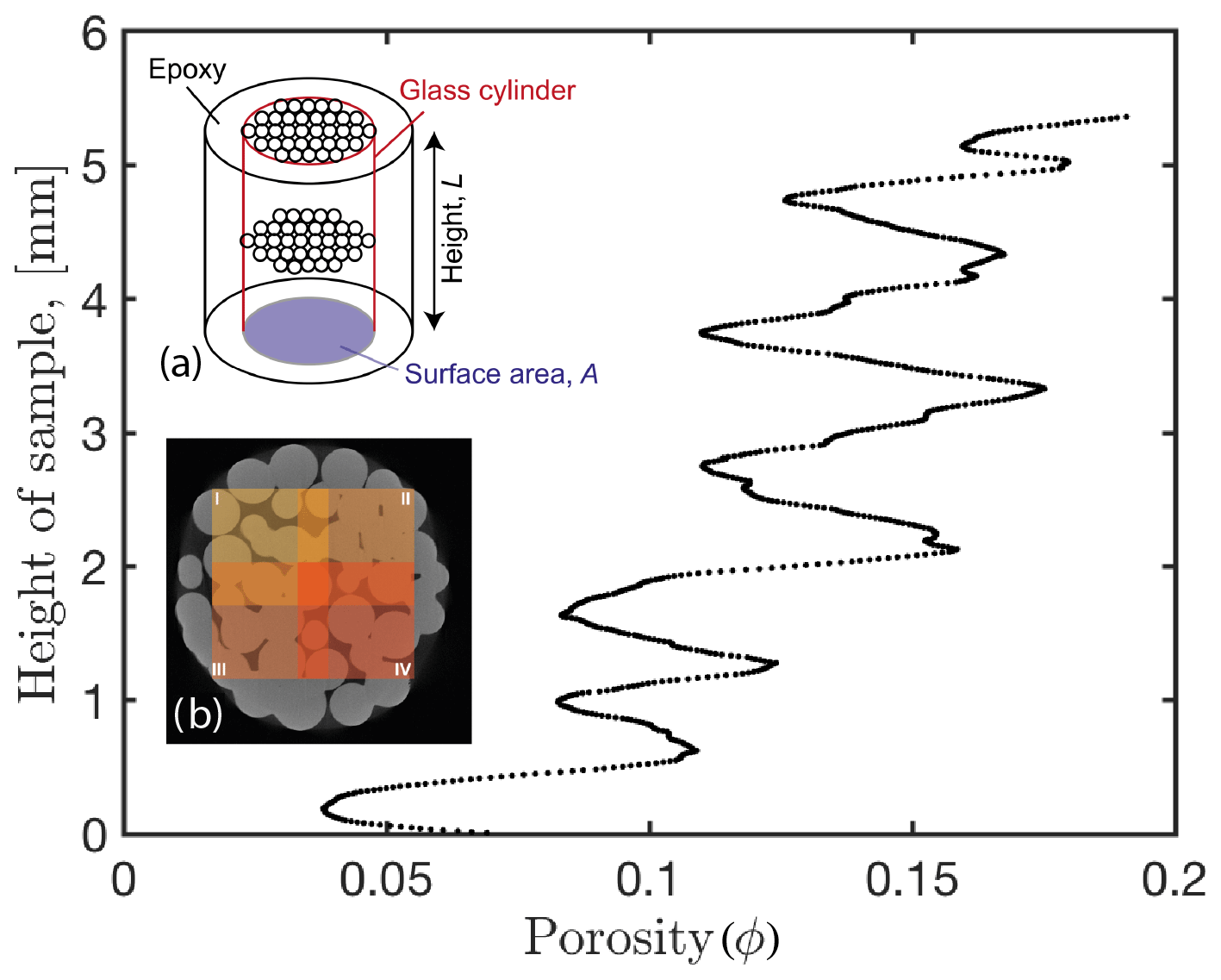
Figure 2Computed porosity of each CT slice from the top to the bottom of a full sample (z axis; sample Ex14). The diagram shows that gravity affects the porosity of the sample. Porosity minima correspond to distinct layers of glass bead within the sample. The inset (a) provides a sketch of the sample structure. In the inset, red outlines the cylindrical shape, blue the surface area A of the cylinder and L the height of the sample. (b) Chosen locations for the squared subsamples 1–4. Four additional subsamples (5–8) are similarly placed below subsamples 1–4 overlapping in the z direction.
2.2 Experimental permeability measurement
In a first preparation step we wrap a highly viscous commercial water-resistant resin around the sample to avoid pore space infiltration. In a next step we embed the sample within a less viscous resin (Technovit 4071 from Heraeus Kulzer GmbH or Presin from Nichika Inc.) to create an airtight casing. The upper and lower surface of the sample were ground and polished to prevent leaks during experimental permeability measurements (Fig. 1; “Sample preparation”).
The experimental permeability measurements were conducted at Tohoku University using a permeameter, described in Takeuchi et al. (2008) and Okumura et al. (2009). To determine permeability the airflow through a sample is measured at room temperature. The pressure gradient between the sample inlet and outlet is controlled by a pressure regulator (RP1000-8-04, CKD Co.; precision ±0.1 %) at the inlet side. To monitor the pressure difference a digital manometer (testo526-s, Testo Inc.; precision ±0.05 %) is used. Airflow through the sample is measured using a digital flowmeter (Alicat, M-10SCCM; precision ±0.6 %). As Darcy's law assumes a linear relationship between the pressure and flow rate, we measure the gas flow rate at several pressure gradients (see Fig. C1 in Appendix C) to verify our assumption of laminar flow conditions. The permeability of all samples is calculated using Darcy's law (Eq. 1) based on measured values (Table 1a).
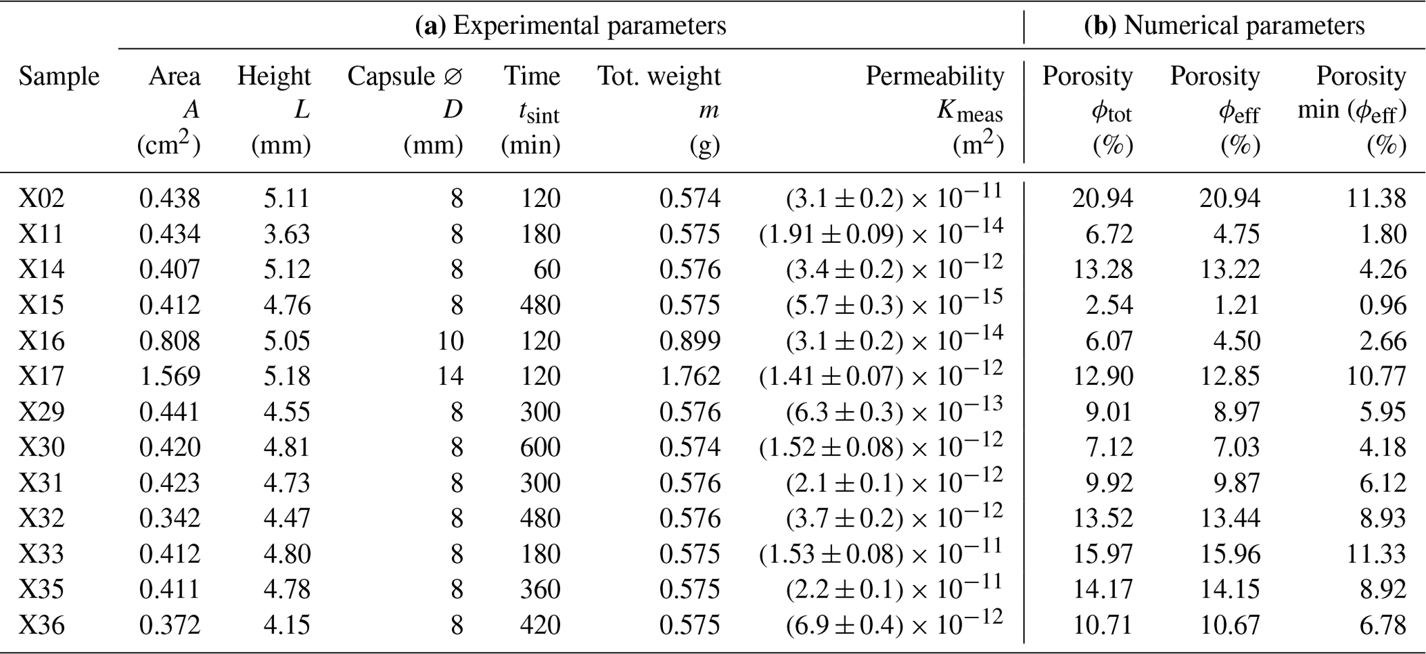
Table 1Column (a) displays the experimental parameters of sintering conditions and parameters used to compute permeability using Darcy's law. A denotes the sample surface area, L the height of the glass bead cylinders and D the inner diameter of each capsule. Additionally, the sintering time tsint, the total weight of the glass beads m and the experimentally measured permeability Kmeas are given. In (b), we list the total, effective and minimum effective porosity – ϕtot, ϕeff and min(ϕeff) – of each sample. These porosities have been obtained with image processing (see Sect. 2.4).
2.3 Micro-CT images and segmentation
Before preparing the samples for permeability measurements all samples are digitized using micro-computed tomographic scans (micro-CT) performed at Tohoku University (ScanXmate-D180RSS270) with a resolution of ≈6–10 µm according to the method of Okumura and Sasaki (2014). Andrä et al. (2013b) showed that the process of segmentation of micro-CT images may have a significant effect on the three-dimensional pore space and therefore the computed flow field. In two-phase systems (fluid + mineral), as in this study, the segmentation is straightforward due to the high contrast in absorption coefficients between glass beads and air, while it can become quite complex for multiphase systems featuring several mineral phases. In the present study the segmentation of the obtained micro-CT images was done using built-in MATLAB functions. In a first step the images are binarized using Otsu's method (Otsu, 1979). Additional smoothing steps of the images are performed. In a next step the two-dimensional micro-CT slices are stacked on top of each other, resulting in a three-dimensional representation of the pore space (Fig. 1; “3D structure”).
2.4 Porosity determination
Porosity is an important parameter describing microstructures. It is defined as the ratio of the total pore space VV to the bulk volume of the sample Vb (Bird et al., 2006):
In a first step, the total porosity of each sample is determined by counting the number of solid and fluid voxels. In a second step, we determine the isolated pore space using a flooding algorithm implemented in MATLAB (bwconncomp). This isolated pore space is then subtracted from the total pore space to obtain an effective pore space Veff. As a bonus, this procedure reduces the computational cost for numerical permeability determinations by removing the parts of the pore space that do not contribute to fluid flow and thus permeability. The effective porosity ϕeff is then defined as the volume of all percolating pore space clusters to the bulk volume of the sample:
It should be mentioned that in a simple capillary model ϕeff=ϕ since no isolated pore space exists. It should also be noted that only the effective porosity is used to determine microstructural and flow properties later in this study.
As described in Sect. 2.1, the porosity of the samples is not homogeneous but increases towards the sample bottom due to gravity. As permeability may not necessarily be affected by the total porosity, but rather by the minimum effective porosity in a sample (in a slice perpendicular to the flow direction), we also determined the minimum effective porosity of each sample (see Table 1b).
2.5 Effective specific surface
The specific surface is defined as the total interfacial surface area of pores As per unit bulk volume Vb of the porous medium (Bear, 1988):
As in the previous section we compute the effective specific surface of all percolating pore space clusters and neglect isolated pore space. To determine the effective specific surface we use the extracted connected clusters and compute an isosurface of the entire three-dimensional binary matrix. In a next step the area of the resulting isosurface As is calculated.
2.6 Numerical method
The relationship between inertial and viscous forces in fluid flows is described by the Reynolds number:
where ρ is the density, v the velocity component, L denotes the length of the domain and η is the viscosity of the fluid. For laminar flow conditions (Re<1; see Fig. C1 Appendix C) and ignoring gravity, the flow in porous media can be described with the incompressible Stokes equations:
with P being the pressure and x the spatial coordinate. For all simulations, we employed a fluid viscosity of 1 Pa s.The Stokes equations are solved using the finite-difference code LaMEM (Kaus et al., 2016; Eichheimer et al., 2019a). LaMEM employs a staggered-grid finite-difference scheme (Harlow and Welch, 1965), whereby pressures P are defined at the cell centres and velocities v at cell faces. Based on the data from the CT scans, each cell is assigned either a fluid or a solid phase. The discretized system of equations is then solved using multigrid solvers of the PETSc library (Balay et al., 2019). As only cells within the fluid phase contribute to fluid flow the discretized governing equations are only solved for these cells. This greatly decreases the number of degrees of freedom and therefore significantly reduces the computational cost. Due to computational limitations and the densification at the bottom of the samples (see Fig. 2) we extract eight overlapping subvolumes per full sample (see Fig. 2b) with sizes of 5123 cells. For each subvolume we compute effective porosity, effective specific surface, hydraulic tortuosity and permeability.
2.7 Numerical permeability computation
From the calculated velocity field in the z direction the volume-averaged velocity component vm is calculated (e.g. Osorno et al., 2015):
where Vf is the volume of the fluid phase. Using Darcy's law (Eq. 1; Andrä et al., 2013a; Bosl et al., 1998; Morais et al., 2009; Saxena et al., 2017) an intrinsic permeability ks is computed via
2.8 Hydraulic tortuosity
Tortuosity is not only highly relevant for the Kozeny–Carman relation, but is also used in various engineering and science applications (Nemati et al., 2020). It has a major influence on liquid-phase mass transport (e.g. in Li-ion batteries, Thorat et al., 2009, and membranes Manickam et al., 2014), the effectiveness of tertiary oil recovery (Azar et al., 2008) and the evaporation of water in soils (Hernández-López et al., 2014). In recent years, several definitions for tortuosity have been suggested (Clennell, 1997; Bear, 1988; Ghanbarian et al., 2013). For the remainder of this study we will calculate and apply the so-called hydraulic tortuosity (Ghanbarian et al., 2013). Assuming that hydraulic tortuosity changes with porosity, both numerical and experimental studies have published different relations of hydraulic tortuosity to porosity. In most cases the hydraulic tortuosity is assumed to be constant as it is difficult to determine experimentally, which is rarely done. It should be mentioned that the following hydraulic tortuosity–porosity relations have been obtained for porous media with >30 % porosity.
Matyka et al. (2008) numerically determined the hydraulic tortuosity by using an arithmetic mean given as
where is the hydraulic tortuosity of a flow line crossing through point ri (Eq. 3) and N the total number of streamlines.
Koponen et al. (1996) computed hydraulic tortuosity numerically using
where is the fluid velocity at point ri, and points ri are chosen randomly from the pore space (Koponen et al., 1996).
One of the most common relations for hydraulic tortuosity is a logarithmic function of porosity reading as follows:
where B is a constant found experimentally for different particles (e.g. 1.6 for wood chips – Pech, 1984 and Comiti and Renaud, 1989; 0.86 to 3.2 for plates – Comiti and Renaud, 1989). By numerically computing hydraulic tortuosity for two-dimensional squares, Matyka et al. (2008) obtained B=0.77. A different experimental relation for hydraulic tortuosity measuring the electric conductivity of spherical particles was proposed by Mota et al. (2001):
Numerically investigating two-dimensional porous media with rectangular-shaped particles, Koponen et al. (1996) proposed a different relation:
In the present study the hydraulic tortuosity is determined according to Eq. (17), which requires computing the tortuosity τ of individual streamlines within each sample. Streamlines describe a curve traced out in time by a fluid particle with a fixed mass and are described mathematically as
with v being the computed velocity field obtained from the numerical simulation and t being the time. Integrating Eq. (22) yields
where x0 is the position of the prescribed particle at t=0. Equation (22) is solved using built-in MATLAB ODE (ordinary differential equation) solvers. To compute the streamline length all fluid cells at the inlet of the subsample are extracted and used as streamline starting points. Using the computed velocity field and Eq. (22) the streamline length for each starting point is calculated. Hence, up to 40 000 streamlines need to be computed for a subsample with ≈20 % porosity, whereas for a subsample with ≈5 % porosity up to 5000 streamlines are computed.
In this section we analyse the different samples in terms of porosity, specific surface, hydraulic tortuosity and permeability. All data for each subsample presented here are given in the Supplement tables (see Table S1–S13). Effective porosity and effective specific surface are computed for both subsamples and full samples, whereas hydraulic tortuosities and permeabilities are only computed for subsamples due to computational limitations. In the present study we analysed 13 samples and 104 subsamples.
3.1 Porosity
The total porosity for each sample and subsample is analysed using image processing and ranges from 2.5 % to 21 % (see Tables 1b and S1–S13). The effective porosity is determined by extracting all connected clusters within the samples and ranges from 1.21 % to 21 % (see also Table 1b). The analysis of the micro-CT images also showed that during sintering densification of the samples occurs (see Fig. 2). For this reason we furthermore report the minimum effective porosity min(ϕeff). Assuming an effective porosity for the entire sample therefore does not seem to be representative. As during the laboratory measurements a first-order control mechanism of the fluid flow and therefore permeability is the lowest porosity within the entire sample.
3.2 Effective specific surface
Figure 3 shows the computed specific surfaces for all subsamples and all full samples with increasing effective porosity. Koponen et al. (1997) used the following relationship to predict the specific surface:
where n is the dimensionality and R0 is the hydraulic radius of the particles. The hydraulic radius is defined as 2Vp∕M (e.g. Bernabé et al., 2010), with Vp being the pore volume and M being the pore surface area. For a regular simple cubic sphere packing with ϕ=0.476 the estimated hydraulic radius is ≈151 µm. To relate the computed values for the effective specific surface to the effective porosity, the above equation is fitted, resulting in a hydraulic radius of 385.09 µm:
The fit between Eq. (24) and our data shows good agreement, which is also reflected in a value of R2=0.975 (see Fig. 3).
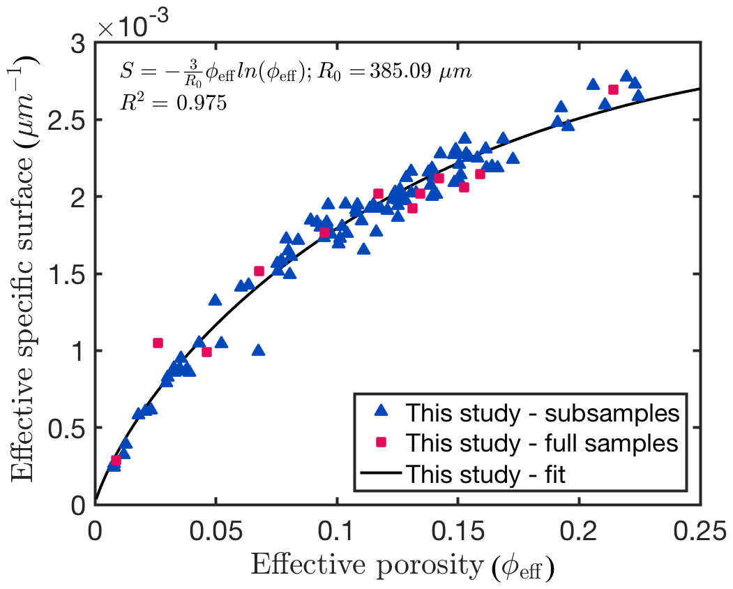
Figure 3Effective specific surface as a function of effective porosity. Blue triangles represent subsample data from this study and red squares the effective specific surface of full samples. Full sample data points are plotted in order to show that in terms of effective specific surface subsamples represent full samples very well. The black curve represents the fitted curve according to Eq. (25).
3.3 Hydraulic tortuosity
We computed hydraulic tortuosities for all subsamples which exhibit a percolating pore space. Results are shown in Fig. 4, where we compare different hydraulic tortuosity–porosity parameterizations presented in Sect. 2.8 to our data. In Fig. 4a–c, we compare our data (denoted by grey squares) with one of the three porosity–hydraulic tortuosity parameterizations (denoted by solid and dashed lines), whereas in Fig. 4d, we show a simple linear fit to our data. In general, computed hydraulic tortuosities are quite scattered and show variations ranging from values of about 2 to values of around 4. In Fig. 4a we compare our data to the hydraulic tortuosity parameterization from Matyka et al. (2008) (see Eq. 19), which is denoted by a dashed black line. We refitted this parameterization using our data; the result is shown by the red solid line, with corresponding 95 % confidence bounds and a coefficient of determination . In Fig. 4b and c, similar comparisons are shown but for the parameterizations by Koponen et al. (1996) (Fig. 4b) and Mota et al. (2001) (Fig. 4c). In both cases, we show the original parameterizations as a black dashed line and the fitted parameterizations as a coloured solid line, with coloured dashed lines indicating the 95 % confidence bounds. As for the parameterization by Matyka et al. (2008), these two parameterizations do not fit our data very well, as also indicated by their low R2 values ( and R2=0.0758, respectively). Finally, in Fig. 4c, we show a linear fit to our data together with the 95 % confidence bounds. As indicated by the low R2 value of 0.0274, this fit also does not represent the data very well. For this reason we use the arithmetic mean of the computed hydraulic tortuosities for later permeability predictions. Nevertheless, we do observe that despite the large scatter, hydraulic tortuosity largely remains relatively constant with decreasing porosity, thus indicating that the pore distribution of our experimental products is homogeneous and the geometrical similarity of pore structure was kept during sintering. This is in contrast to the parameterizations of Matyka et al. (2008) and Mota et al. (2001), both predicting a significant increase in tortuosity as small porosities are approached, but agrees with the model of Koponen et al. (1996).
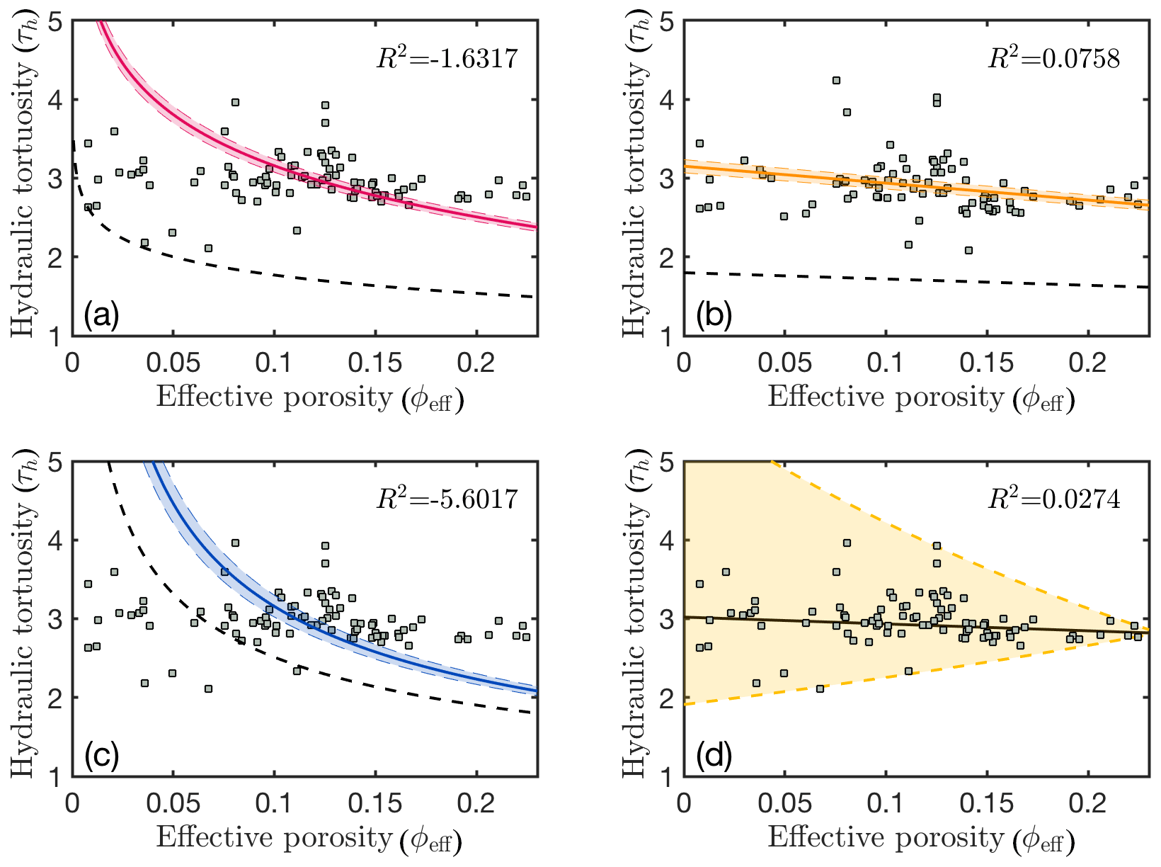
Figure 4Panels (a)–(c) show the proposed relations for the hydraulic tortuosity according to (a) Matyka et al. (2008), (b) Koponen et al. (1996) and (c) Mota et al. (2001) as black dashed lines. The coloured solid lines represent the fit of the computed data to those relations within the 95 % confidence bounds. Hydraulic tortuosities for all subsamples (grey squares) are computed according to the method used in each of these studies. Panel (d) shows the fit obtained in the present study. The coloured area in (d) illustrates the extending distribution of computed hydraulic tortuosities with decreasing effective porosity.
3.4 Permeability
In Fig. 5, measured permeabilities for all samples are shown as grey symbols (see also Table 1a for measured values). We chose to plot sample permeabilities vs. the minimum of the effective porosity here, the reason being the intrinsic porosity variations in each sample (see Sect. 2.4). Figure A1 in the Appendix shows both the effective porosity and minimum effective porosity of each sample.
Measured permeabilities range from values of around 10−14 to about 10−11 m2, depending on porosity. Although experimental measurements are scattered, a clear trend can be observed. At porosities close to the critical porosity, permeabilities are very low but rapidly increase when porosities increase slightly. At larger porosities, permeabilities further increase, but this increase is significantly less rapid.
Numerically, 98 subsamples have been computed successfully with permeabilities ranging from around 10−14 to about 10−10 m2, depending on porosity (see Tables S1–S13 and Fig. B1 in the Appendix). In comparison to the experimentally measured samples, the numerical permeabilities tend towards higher values but show a clear trend.
As we split each sample in eight subsamples for numerical permeability computations, we need to average them to compute an effective sample permeability that can then be compared to measured values. This upscaling issue is not trivial to address, and it is not clear yet which averaging method is appropriate. It is possible to put bounds on the effective permeability by using either the arithmetic or harmonic mean of subsample permeabilities. However, these bounds correspond to very specific geometrical sample structures. In the case of the arithmetic mean, the medium is assumed to consist of parallel layers oriented parallel to the flow direction, whereas the harmonic mean is valid in the case of parallel layers orthogonal to the flow direction. This is most often not the case. Therefore, different averaging methods have been developed to obtain adequate upscaling procedures for heterogeneous porous media (e.g. Sahimi, 2006; Jang et al., 2011; Torquato, 2013). One of the simplest averaging schemes that has been shown to be an appropriate approximation for heterogeneous porous media is the geometric mean (e.g. Warren and Price, 1961; Selvadurai and Selvadurai, 2014; Jang et al., 2011), which reads as
where i is the number of the subsample and n the total number of subsamples (eight in this study). As several subsamples at low porosities did not exhibit a connected pore space (thus not allowing for any fluid flow), we assumed a permeability of 10−20 m2 for these samples. The geometric averages of each subsample set are shown in Fig. 5.
To determine the predictive power of the different permeability parameterizations described in Sect. 1, we inserted the expressions for effective specific surface and hydraulic tortuosity into the respective equations (Eqs. 4 and 5). The Kozeny–Carman equation then reads as
with k0=0.5 being the geometrical parameter for spherical particles (Kozeny, 1927) and ϕc=0.01 the critical porosity threshold. This threshold is lower than the published value of ϕc=0.03 (Van der Marck, 1996; Rintoul, 2000; Wadsworth et al., 2016). However, one of the subsamples used in this study had a porosity of 0.01 while still exhibiting a percolating cluster. For this reason, we employed a critical porosity of ϕc=0.01.
With our parameterization for S, the permeability parameterization of Martys et al. (1994) reads as follows:
From the grain size distribution of the glass beads used in this study (see Appendix D), we also determined the average grain diameter d and the harmonic mean diameter D, both within uncertainties equal to 1.20 mm. Inserting into the respective parameterizations of Revil and Cathles (1999) and Garcia et al. (2009) (see Eqs. 7 and 8) results in
The permeability parameterizations in general show similar trends but differ in the predicted permeability value. The Kozeny–Carman relation shows good agreement with the experimentally measured samples but also shows some offset towards the numerically computed values. A similarly good fit is obtained by the permeability parameterization of Martys et al. (1994). The parameterizations by Garcia et al. (2009) and Revil and Cathles (1999) tend to underestimate permeability, which might be related to their assumptions on the sample heterogeneity.
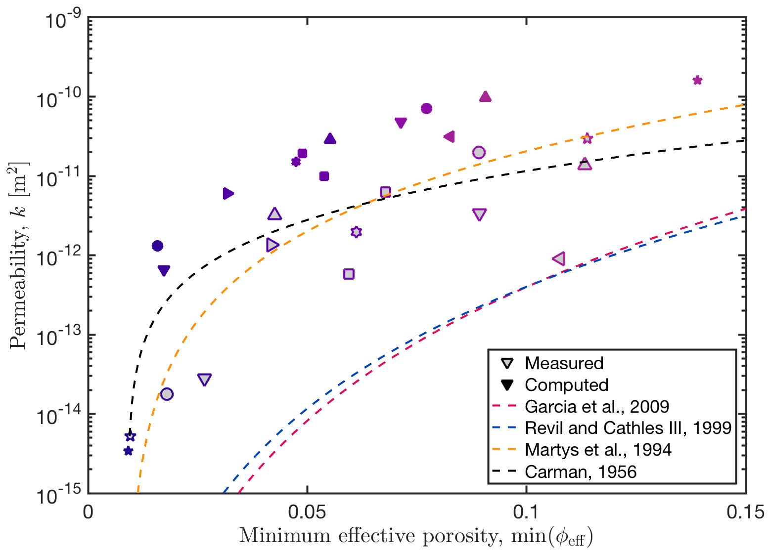
Figure 5Computed and measured permeability against minimum effective porosity. Symbols of the same shape and colour represent the same sample. Samples with a grey face represent measured values, whereas colour-only symbols stand for computed subsamples. The computed permeabilities represent the geometric mean values of all subsamples. To verify existing permeability parameterizations, we plotted the relations of Revil and Cathles (1999), Garcia et al. (2009), Carman (1956), and Martys et al. (1994) against the experimental and numerical permeabilities. Note that estimated errors for the experimental permeability measurements (Table 1a) are smaller than the displayed symbols. Some subsamples with low effective porosity did not show a continuous pathway throughout the subsample, and thus we assumed a very low permeability of 10−20 m2.
In this paper, we determine the permeability of nearly isotropic porous media consisting of sintered glass beads using a combined experimental–numerical approach. We analysed sample microstructures using CT data and determined flow properties both experimentally and numerically. Using these data, we test different permeability parameterizations that have been proposed in the literature. The goal of this study was to particularly improve permeability parameterizations at low porosities (<20 %).
Two particular microstructural parameters that we determined were the specific surface S and the hydraulic tortuosity τh. As these two parameters are frequently used in permeability parameterizations, we tested whether existing parameterizations are also valid in our case. We find that the effective specific surface is well predicted by the parameterization in Eq. (24) proposed by Koponen et al. (1996), not only for the chosen subsamples but also for the full samples. The fitted hydraulic radius of 0.385 mm is reasonable as the initial grain size of the glass beads is around 1 mm and the hydraulic pore radius of the glass beads is reduced during sample sintering.
Only a few studies have investigated hydraulic tortuosity for three-dimensional porous media (Du Plessis and Masliyah, 1991; Ahmadi et al., 2011; Backeberg et al., 2017). As the hydraulic tortuosity is challenging to determine in experiments, experimental studies have often used this parameter as a fitting variable. Our data show that – contrary to previous suggestions – the hydraulic tortuosity does not change significantly with decreasing effective porosity (Matyka et al., 2008; Koponen et al., 1996; Mota et al., 2001), at least at the low porosities investigated in this study. This observation agrees with the study by Koponen et al. (1996) but is at odds with the studies by Matyka et al. (2008) and Mota et al. (2001). The study by Koponen et al. (1996) was based on 2D numerical simulations and found hydraulic tortuosity values close to 2, whereas our data lie around a value of 3. The difference between previous relations and our data is likely related to the different particle geometries used and the fact that previous studies were done in 2D, while we employ 3D samples.
Measured and computed permeabilities are generally in good agreement, with computed permeabilities consistently yielding higher values than experimentally measured permeabilities. The experimentally measured permeabilities show some scatter, which might be related to heterogeneities within the sample. Interestingly, numerical permeability computations based on subsamples show much less scatter. Both the modified Kozeny–Carman relation and the parameterization by Martys et al. (1994) predict numerically computed and experimentally measured permeability values well. In the modified Kozeny–Carman relation, hydraulic tortuosity seems to have a second-order influence on the permeability of porous media. The permeability parameterizations by Revil and Cathles (1999) and Garcia et al. (2009) underestimate permeabilities, which could be related to the assumptions used in these studies. It should be noted that Garcia et al. (2009) investigated heterogeneous sand packs and found that permeabilities for homogeneous packs are 1.6–1.8 times higher.
There are several reasons for the discrepancy between experimental and numerical values. First, numerical permeability predictions are based on simulations on subsamples for which free-slip boundary conditions are employed. These boundary conditions do not accurately represent the flow field within the full sample and are therefore a possible source of error. This error can be estimated to about 20 %–50 % of the computed value (Gerke et al., 2019). Second, the numerical computations compute the flow field on a discretized grid with a given resolution. In particular at low porosities, pore structures may be too small to be well resolved by the grid. As discussed by previous studies the accuracy of permeability prediction improves with increasing numerical resolution (Gerke et al., 2018; Keehm, 2003; Eichheimer et al., 2019a). To investigate this effect with respect to our samples, we computed the permeability of two subsamples (Ex35Sub04 and Ex36Sub02; see the Supplement) using an increased resolution of 10243 grid points. The two samples with effective porosities at around 9 % and 15 % represent samples on both sides of the median of the present study's effective porosity range (1.5 %–22 %). The permeability obtained using doubled grid resolution decreases only by around ≈2 %–4 % compared to the outcome of models with 5123 grid resolution (see Appendix F). We are therefore confident that the calculations with 5123 grid points provide sufficiently accurate results. To further increase the accuracy of the numerical computations, adaptive meshing methods could be useful.
Third and most important, it is not clear whether either the subsamples used in the numerical computations or the full samples used for experimental measurements can be considered representative volume elements at a certain porosity. The scatter that we observe in both numerical and experimental permeability measurements indicates that this may not be the case, in particular at porosities close to the critical porosity. A potential remedy for this issue would be the use of larger samples in both experiments and numerical simulations. However, using larger samples is not trivial. On the numerical side larger samples require significantly more computational resources. On the experimental side, larger samples reduce the resolution of the CT scans, which would in turn reduce the value of microstructural analysis. Additionally, a reduced CT resolution would also affect numerical permeability measurements.
We show that several permeability parameterizations (the modified Kozeny–Carman equation and the permeability parameterization by Martys et al., 1994) are capable of predicting the numerically and experimentally determined permeabilities obtained in our study. However, this could only be done by determining several microstructural parameters from CT scans and by modifying the respective equations to fit our data. In that respect, the parameterization by Martys et al. (1994) requires fewer fitting parameters, which makes it preferable in our opinion. However, our results also show a significant scatter in both numerical and experimental permeability measurements, which is not predicted by either parameterization. This shows that further work is needed to obtain a more universal parameterization connecting microstructural parameters to permeability. To first order, different permeability parameterizations can be used in numerical models to simulate fluid flow in isotropic low-porosity media on a larger scale. However, it has to be kept in mind that rocks in nature are commonly more complex, as they (1) often consist of grains with different shapes and sizes, (2) contain fractures which serve as preferred pathways for fluid flow, and (3) often also contain anisotropic structures.
Nevertheless, our study demonstrates that numerical permeability computations can complement laboratory measurements, in particular in cases of small sample sizes or effective porosities <5 %. We provide segmented input files of several samples with different porosities in the Supplement. We hope that this will allow other researchers to use these data and our results to benchmark other numerical methods in the future.
Figure A1 shows the comparison between the effective porosity and the minimum effective porosity, which may control the fluid flow within the sample. The minimum effective porosity is used in Fig. 5.

Figure A1Measured permeability against porosity. Symbols with a grey face represent a sample using the minimum effective porosity per sample, while red symbols display a measured sample using the effective porosity. Dashed lines show several permeability parameterizations.
Figure B1 shows the computed permeability of each subsample together with the measured permeability values and the permeability parameterizations.
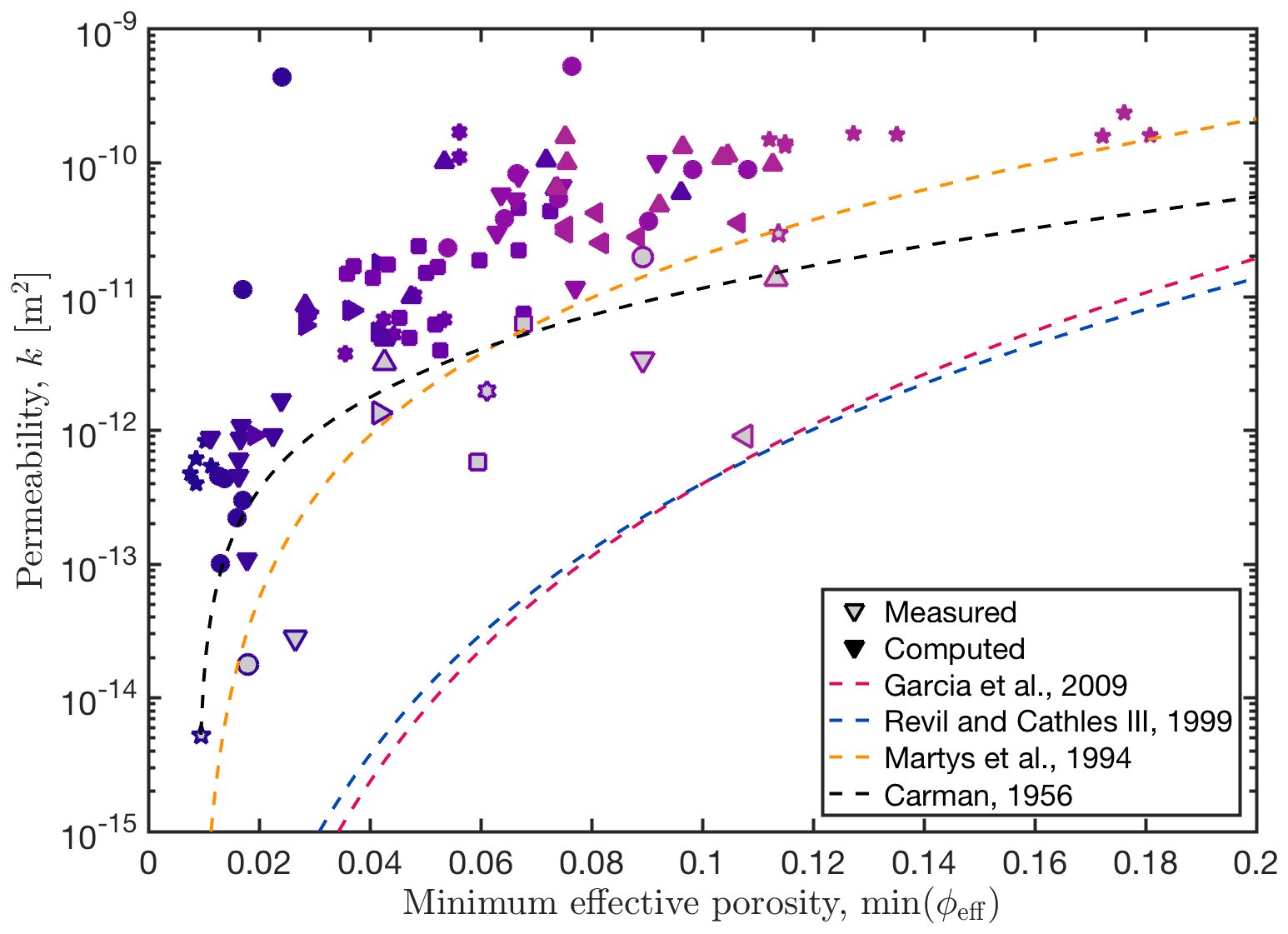
Figure B1Computed and measured permeability against minimum effective porosity. Symbols of the same shape and colour represent the same sample. Samples with a grey face represent measured values, whereas colour-only symbols stand for computed subsamples. To verify existing permeability parameterizations, we plotted the relations of Revil and Cathles (1999), Garcia et al. (2009), Carman (1956), and Martys et al. (1994) against the experimental and numerical permeabilities. Note that estimated errors for the experimental permeability measurements (Table 1a) are smaller than the displayed symbols.
For the numerical permeability computation using the Stokes equations we assume laminar flow conditions and incompressibility. Laminar flow conditions are represented by a linear relationship between the applied pressure gradient and flow rate (Fig. C1). Regarding the incompressibility of the working gas during the measurements we computed permeabilities using both Darcy's law (Eq. 1) and Darcy's law for compressible gas as follows (Takeuchi et al., 2008):
with P2 and P1 being the pressures at the inlet and outlet side of the sample, respectively, and ν0 being the volume flux, which is calculated from the flow rate divided by the cross-sectional area of the sample. The left-hand side of Eq. (C1) represents the modified pressure gradient that includes the compressibility of the working gas. The difference between the two computed permeabilities is less than 10 %, and we therefore assume the effect of compressibility to be minor.
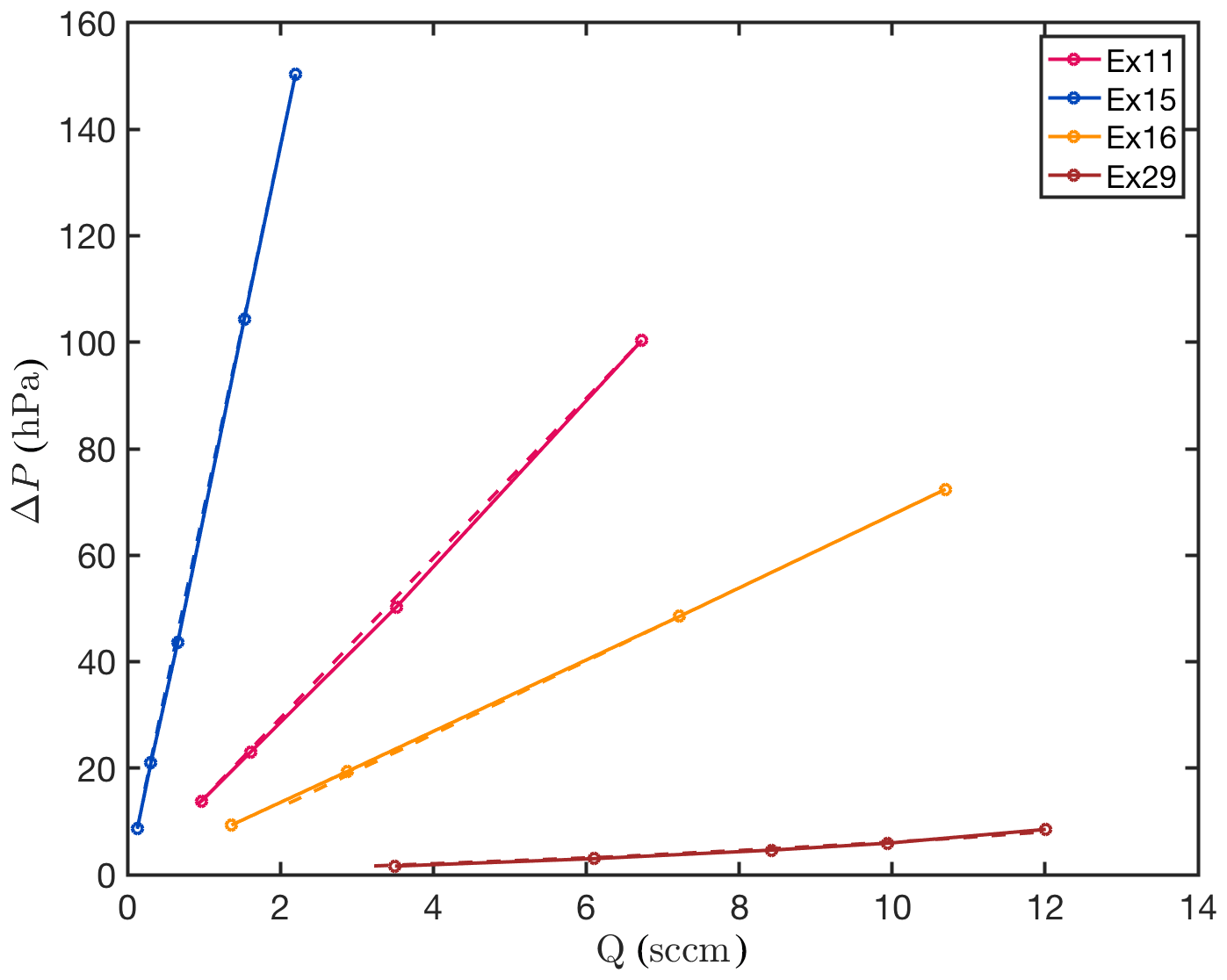
Figure C1The linear relations between applied pressure difference and flow rate show that Darcy's law is valid and no turbulent flow occurs. Solid lines represent measurements while increasing the pressure difference, and dashed lines represent decreasing the pressure difference (sccm: standard cubic centimetres per minute).
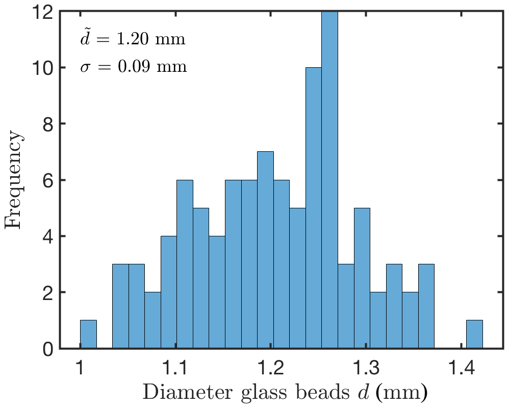
Figure D1Size frequency distribution of the glass bead diameters. In addition to the distribution, both the arithmetic mean and standard deviation σ are given.
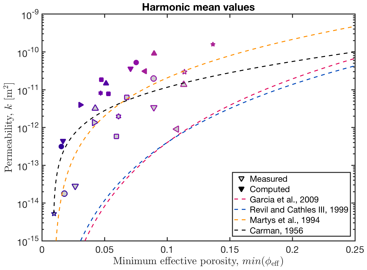
Figure E1Computed and measured permeability against minimum effective porosity. Symbols of the same shape and colour represent the same sample. Samples with a grey face represent measured values, whereas colour-only symbols stand for computed subsamples. The computed permeabilities represent the harmonic mean values of all subsamples. To verify existing permeability parameterizations, we plotted the relations of Revil and Cathles (1999), Garcia et al. (2009), Carman (1956), and Martys et al. (1994) against the experimental and numerical permeabilities. Note that estimated errors for the experimental permeability measurements (Table 1a) are smaller than the displayed symbols.
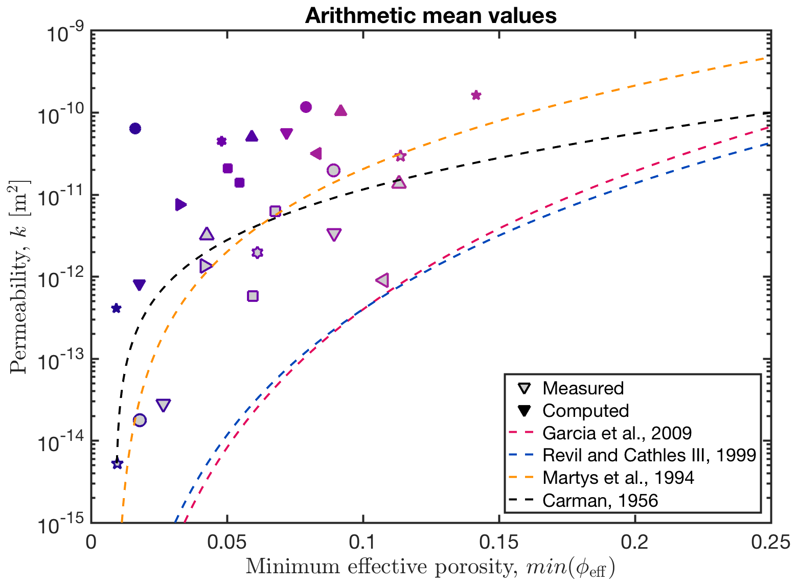
Figure E2Computed and measured permeability against minimum effective porosity. Symbols of the same shape and colour represent the same sample. Samples with a grey face represent measured values, whereas colour-only symbols stand for computed subsamples. The computed permeabilities represent the arithmetic mean values of all subsamples. To verify existing permeability parameterizations, we plotted the relations of Revil and Cathles (1999), Garcia et al. (2009), Carman (1956), and Martys et al. (1994) against the experimental and numerical permeabilities. Note that estimated errors for the experimental permeability measurements (Table 1a) are smaller than the displayed symbols.

Figure F1Resolution test using samples Ex35Sub04 and Ex36Sub02 (for details, see also tables in the Supplement). Coloured squares denote a standard resolution of 5123, whereas coloured triangles are simulations with a resolution of 10243 voxels.
The code is available at https://bitbucket.org/bkaus/lamem/src/master/ (commit: 9c06e4077439b5492d49d03c27d3a1a5f9b65d32) (Popov and Kaus, 2016).
Detailed data tables for each sample can be found in the Supplement. The segmented CT images of three samples with different porosities are provided using the figshare repository (https://doi.org/10.6084/m9.figshare.11378517; Eichheimer et al., 2019b).
The supplement related to this article is available online at: https://doi.org/10.5194/se-11-1079-2020-supplement.
PE contributed to designing the study, sample preparation and permeability measurements. Furthermore, PE conducted visualization, writing, methodology and running simulations. MT contributed to data interpretation, methodology, designing the study and paper writing. WF performed sample preparation and permeability measurements. GJG contributed to designing the study, data interpretation and paper writing. MN designed the study and contributed to data interpretation. SO contributed to sample preparation and measurements. TK sintered the glass bead porous media. MOK performed the resolution test. All authors contributed to writing and improving the paper.
The authors declare that they have no conflict of interest.
Additionally, this work has been supported by the JSPS Japanese–German graduate externship. Marcel Thielmann was supported by the Bayerisches Geoinstitut Visitors Program. Calculations were performed on the clusters btrzx2 at the University of Bayreuth and Mogon II at Johannes Gutenberg University Mainz. We thank Kirill Gerke and an anonymous reviewer for their constructive comments that helped to improve the paper considerably.
This research has been supported by the DFG (grant no. GRK 2156/1) and the BMBF (grant no. 03G0865A).
This open-access publication was funded
by the University of Bayreuth.
This paper was edited by Cristiano Collettini and reviewed by Kirill Gerke and one anonymous referee.
Ahmadi, M. M., Mohammadi, S., and Hayati, A. N.: Analytical derivation of tortuosity and permeability of monosized spheres: A volume averaging approach, Phys. Rev. E, 83, 026312, https://doi.org/10.1103/PhysRevE.83.026312, 2011. a
Andrä, H., Combaret, N., Dvorkin, J., Glatt, E., Han, J., Kabel, M., Keehm, Y., Krzikalla, F., Lee, M., Madonna, C., Marsh, M., Mukerji, T., Saenger, E. H., Sain, R., Saxena, N., Ricker, S., Wiegmann, A., and Zhan, X.: Digital rock physics benchmarks–Part II: Computing effective properties, Comput. Geosci., 50, 33–43, https://doi.org/10.1016/j.cageo.2012.09.008, 2013a. a, b, c
Andrä, H., Combaret, N., Dvorkin, J., Glatt, E., Han, J., Kabel, M., Keehm, Y., Krzikalla, F., Lee, M., Madonna, C., Marsh, M., Mukerji, T., Saenger, E. H., Sain, R., Saxena, N., Ricker, S., Wiegmann, A., and Zhan, X.: Digital rock physics benchmarks–Part I: Imaging and segmentation, Comput. Geosci., 50, 25–32, https://doi.org/10.1016/j.cageo.2012.09.005, 2013b. a
Arns, C. H.: A comparison of pore size distributions derived by NMR and X-ray-CT techniques, Physica A, 339, 159–165, https://doi.org/10.1016/j.physa.2004.03.033, 2004. a
Arns, C. H., Knackstedt, M. A., Pinczewski, M. V., and Lindquist, W.: Accurate estimation of transport properties from microtomographic images, Geophys. Res. Lett., 28, 3361–3364, https://doi.org/10.1029/2001GL012987, 2001. a
Azar, J. H., Javaherian, A., Pishvaie, M. R., and Nabi-Bidhendi, M.: An approach to defining tortuosity and cementation factor in carbonate reservoir rocks, J. Petrol. Sci. Eng., 60, 125–131, https://doi.org/10.1016/j.petrol.2007.05.010, 2008. a
Backeberg, N. R., Lacoviello, F., Rittner, M., Mitchell, T. M., Jones, A. P., Day, R., Wheeler, J., Shearing, P. R., Vermeesch, P., and Striolo, A.: Quantifying the anisotropy and tortuosity of permeable pathways in clay-rich mudstones using models based on X-ray tomography, Sci. Rep.-UK, 7, 14838, https://doi.org/10.1038/s41598-017-14810-1, 2017. a
Balay, S., Abhyankar, S., Adams, M. F., Brown, J., Brune, P., Buschelman, K., Dalcin, L., Dener, A., Eijkhout, V., Gropp, W. D., Karpeyev, D., Kaushik, D., Knepley, M. G., May, D. A., McInnes, L. C., Mills, R. T., Munson, T., Rupp, K., Sanan, P., Smith, B. F., Zampini, S., Zhang, H., and Zhang, H.: PETSc Users Manual, Tech. Rep. ANL-95/11 – Revision 3.12, Argonne National Laboratory, available at: https://www.mcs.anl.gov/petsc, last access: 15 December 2019. a
Bear, J.: Dynamics of Fluids in Porous Media, Dover Publications Inc., New York, 1988. a, b, c, d
Bekins, B. A. and Dreiss, S. J.: A simplified analysis of parameters controlling dewatering in accretionary prisms, Earth Planet. Sc. Lett., 109, 275–287, https://doi.org/10.1016/0012-821X(92)90092-A, 1992. a
Berg, R. R.: Capillary Pressures in Stratigraphic Traps, AAPG Bull., 59, 939–956, https://doi.org/10.1306/83D91EF7-16C7-11D7-8645000102C1865D, 1975. a
Bernabe, Y., Brace, W., and Evans, B.: Permeability, porosity and pore geometry of hot-pressed calcite, Mech. Mater., 1, 173–183, https://doi.org/10.1016/0167-6636(82)90010-2, 1982. a
Bernabé, Y., Li, M., and Maineult, A.: Permeability and pore connectivity: A new model based on network simulations, J. Geophys. Res.-Sol. Ea., 115, B10, https://doi.org/10.1029/2010JB007444, 2010. a
Bird, R., Stewart, W., and Lightfoot, E.: Transport Phenomena, New York, London, Wiley, revised second Edition, 2006. a
Bird, M., Butler, S. L., Hawkes, C., and Kotzer, T.: Numerical modeling of fluid and electrical currents through geometries based on synchrotron X-ray tomographic images of reservoir rocks using Avizo and COMSOL, Comput. Geosci., 73, 6–16, https://doi.org/10.1016/j.cageo.2014.08.009, 2014. a
Bosl, W. J., Dvorkin, J., and Nur, A.: A study of porosity and permeability using a lattice Boltzmann simulation, Geophys. Res. Lett., 25, 1475–1478, https://doi.org/10.1029/98GL00859, 1998. a
Bourbie, T., Coussy, O., Zinszner, B., and Junger, M. C.: Acoustics of Porous Media, J. Acoust. Soc. Am., 91, 3080–3080, 1992. a
Brace, W. F.: Permeability of crystalline and argillaceous rocks, International Journal of Rock Mechanics and Mining Sciences & Geomechanics Abstracts, 17, 241–251, https://doi.org/10.1016/0148-9062(80)90807-4, 1980. a
Carman, P. C.: Fluid flow through granular beds, Trans. Inst. Chem. Eng., 15, 150–166, 1937. a, b, c, d, e
Carman, P. C.: Flow of gases through porous media, New York, Academic Press, 1956. a, b, c, d, e, f, g, h
Chapuis, R. P. and Aubertin, M.: On the use of the Kozeny–Carman equation to predict the hydraulic conductivity of soils, Can. Geotech. J., 40, 616–628, https://doi.org/10.1139/t03-013, 2003. a
Clennell, M. B.: Tortuosity: A guide through the maze, Geological Society, London, Special Publications, 122, 299–344, 1997. a
Collinson, A. and Neuberg, J.: Gas storage, transport and pressure changes in an evolving permeable volcanic edifice, J. Volcanol. Geoth. Res., 243–244, 1–13, https://doi.org/10.1016/j.jvolgeores.2012.06.027, 2012. a
Comiti, J. and Renaud, M.: A new model for determining mean structure parameters of fixed beds from pressure drop measurements: application to beds packed with parallelepipedal particles, Chem. Eng. Sci., 44, 1539–1545, https://doi.org/10.1016/0009-2509(89)80031-4, 1989. a, b, c
Darcy, H. P. G.: Les Fontaines publiques de la ville de Dijon: exposition et application des principes à suivre et des formules à employer dans les questions de distribution d'eau, Paris, V. Dalamont, 1856. a
Domenico, P. A. and Schwartz, F. W.: Physical and chemical hydrogeology, Wiley, New York, 1998. a
Du Plessis, J. P. and Masliyah, J. H.: Flow through isotropic granular porous media, Transport Porous Med., 6, 207–221, https://doi.org/10.1007/BF00208950, 1991. a
Dvorkin, J., Derzhi, N., Diaz, E., and Fang, Q.: Relevance of computational rock physics, Geophysics, 76, E141–E153, https://doi.org/10.1190/geo2010-0352.1, 2011. a
Eichheimer, P., Thielmann, M., Popov, A., Golabek, G. J., Fujita, W., Kottwitz, M. O., and Kaus, B. J. P.: Pore-scale permeability prediction for Newtonian and non-Newtonian fluids, Solid Earth, 10, 1717–1731, https://doi.org/10.5194/se-10-1717-2019, 2019a. a, b, c
Eichheimer, P., Thielmann, M., Fujita, W., Golabek, G. J., Nakamura, M., Okumura, S., Nakatani, T., and Kottwitz, M. O.: Detailed data tables for each sample and segmented CT images, Figshare, https://doi.org/10.6084/m9.figshare.11378517, 2019b. a
Fehn, U. and Cathles, L. M.: Hydrothermal convection at slow-spreading mid-ocean ridges, Tectonophysics, 55, 239–260, https://doi.org/10.1016/0040-1951(79)90343-3, 1979. a
Garcia, X., Akanji, L. T., Blunt, M. J., Matthai, S. K., and Latham, J. P.: Numerical study of the effects of particle shape and polydispersity on permeability, Phys. Rev. E, 80, 021304, https://doi.org/10.1103/PhysRevE.80.021304, 2009. a, b, c, d, e, f, g, h, i, j, k
Gerke, K. M., Vasilyev, R. V., Khirevich, S., Collins, D., Karsanina, M. V., Sizonenko, T. O., Korost, D. V., Lamontagne, S., and Mallants, D.: Finite-difference method Stokes solver (FDMSS) for 3D pore geometries: Software development, validation and case studies, Comput. Geosci., 114, 41–58, https://doi.org/10.1016/j.cageo.2018.01.005, 2018. a, b, c
Gerke, K. M., Karsanina, M. V., and Katsman, R.: Calculation of tensorial flow properties on pore level: Exploring the influence of boundary conditions on the permeability of three-dimensional stochastic reconstructions, Phys. Rev. E, 100, 053312, https://doi.org/10.1103/PhysRevE.100.053312, 2019. a
Ghanbarian, B., Hunt, A. G., Ewing, R. P., and Sahimi, M.: Tortuosity in porous media: A critical review, Soil Sci. Soc. Am. J., 77, 1461–1477, 2013. a, b
Gleeson, T. and Ingebritsen, S. E.: Crustal Permeability, John Wiley & Sons, Ltd, https://doi.org/10.1002/9781119166573, 2016. a
Harlow, F. H. and Welch, J. E.: Numerical Calculation of Time-Dependent Viscous Incompressible Flow of Fluid with Free Surface, Phys. Fluids, 8, 2182–2189, https://doi.org/10.1063/1.1761178, 1965. a
Hendraningrat, L., Li, S., and Torsæter, O.: A coreflood investigation of nanofluid enhanced oil recovery, J. Petrol. Sci. Eng., 111, 128–138, https://doi.org/10.1016/j.petrol.2013.07.003, 2013. a
Hernández-López, M. F., Gironás, J., Braud, I., Suárez, F., and Muñoz, J. F.: Assessment of evaporation and water fluxes in a column of dry saline soil subject to different water table levels, Hydrol. Process., 28, 3655–3669, https://doi.org/10.1002/hyp.9912, 2014. a
Hölting, B. and Coldewey, W. G.: Hydrogeology, Springer-Verlag GmbH, Berlin, https://doi.org/10.1007/978-3-662-56375-5, 2019. a
Honarpour, M. M.: Relative Permeability Of Petroleum Reservoirs: Boca Raton, Florida, CRC press, 2018. a
Jang, J., Narsilio, G. A., and Santamarina, J. C.: Hydraulic conductivity in spatially varying media–a pore-scale investigation, Geophys. J. Int., 184, 1167–1179, https://doi.org/10.1111/j.1365-246X.2010.04893.x, 2011. a, b
Kaus, B. J. P., Popov, A. A., Baumann, T. S., Püsök, A. E., Bauville, A., Fernandez, N., and Collignon, M.: Forward and Inverse Modelling of Lithospheric Deformation on Geological Timescales, NIC Series, 48, 299–307, 2016. a, b
Keehm, Y.: Computational rock physics: Transport properties in porous media and applications, PhD thesis, Stanford University, 2003. a, b
Keller, T. and Katz, R. F.: The Role of Volatiles in Reactive Melt Transport in the Asthenosphere, J. Petrol., 57, 1073–1108, https://doi.org/10.1093/petrology/egw030, 2016. a
Keller, T. and Suckale, J.: A continuum model of multi-phase reactive transport in igneous systems, Geophys. J. Int., 219, 185–222, https://doi.org/10.1093/gji/ggz287, 2019. a
Klug, C. and Cashman, K. V.: Permeability development in vesiculating magmas: implications for fragmentation, B. Volcanol., 58, 87–100, https://doi.org/10.1007/s004450050128, 1996. a
Koponen, A., Kataja, M., and Timonen, J. v.: Tortuous flow in porous media, Phys. Rev. E, 54, 406–410, https://doi.org/10.1103/PhysRevE.54.406, 1996. a, b, c, d, e, f, g, h, i, j
Koponen, A., Kataja, M., and Timonen, J.: Permeability and effective porosity of porous media, Phys. Rev. E, 56, 3319–3325, https://doi.org/10.1103/PhysRevE.56.3319, 1997. a
Kozeny, J.: Über kapillare Leitung des Wassers im Boden, Royal Academy of Science, Vienna, Proc. Class I, 136, 271–306, 1927. a, b, c
Kuczynski, G. C.: Study of the Sintering of Glass, J. Appl. Phys., 20, 1160–1163, 1949. a
Lamur, A., Kendrick, J. E., Eggertsson, G. H., Wall, R. J., Ashworth, J. D., and Lavallée, Y.: The permeability of fractured rocks in pressurised volcanic and geothermal systems, Sci. Rep.-UK, 7, 6173, https://doi.org/10.1038/s41598-017-05460-4, 2017. a
Manickam, S. S., Gelb, J., and McCutcheon, J. R.: Pore structure characterization of asymmetric membranes: Non-destructive characterization of porosity and tortuosity, J. Membrane Sci., 454, 549–554, https://doi.org/10.1016/j.memsci.2013.11.044, 2014. a
Manwart, C., Aaltosalmi, U., Koponen, A., Hilfer, R., and Timonen, J.: Lattice-Boltzmann and finite-difference simulations for the permeability for three-dimensional porous media, Phys. Rev. E, 66, 016702, https://doi.org/10.1103/PhysRevE.66.016702, 2002. a, b
Martys, N. S., Torquato, S., and Bentz, D. P.: Universal scaling of fluid permeability for sphere packings, Phys. Rev. E, 50, 403–408, https://doi.org/10.1103/PhysRevE.50.403, 1994. a, b, c, d, e, f, g, h, i, j, k, l
Matyka, M., Khalili, A., and Koza, Z.: Tortuosity-porosity relation in porous media flow, Phys. Rev. E, 78, 026306, https://doi.org/10.1103/PhysRevE.78.026306, 2008. a, b, c, d, e, f, g, h, i
Miller, K. J., lu Zhu, W., Montési, L. G., and Gaetani, G. A.: Experimental quantification of permeability of partially molten mantle rock, Earth Planet. Sc. Lett., 388, 273–282, https://doi.org/10.1016/j.epsl.2013.12.003, 2014. a
Morais, A. F., Seybold, H., Herrmann, H. J., and Andrade, J. S.: Non-Newtonian Fluid Flow through Three-Dimensional Disordered Porous Media, Phys. Rev. Lett., 103, 194502, https://doi.org/10.1103/PhysRevLett.103.194502, 2009. a
Mostaghimi, P., Blunt, M. J., and Bijeljic, B.: Computations of Absolute Permeability on Micro-CT Images, Math. Geosci., 45, 103–125, https://doi.org/10.1007/s11004-012-9431-4, 2013. a
Mota, M., Teixeira, J. A., Bowen, W. R., and Yelshin, A.: Binary spherical particle mixed beds: porosity and permeability relationship measurement, The Filtration Society, 17, 101–106, 2001. a, b, c, d, e, f, g
Mueller, S., Melnik, O., Spieler, O., Scheu, B., and Dingwell, D. B.: Permeability and degassing of dome lavas undergoing rapid decompression: An experimental determination, B. Volcanol., 67, 526–538, https://doi.org/10.1007/s00445-004-0392-4, 2005. a, b
Napolitano, A. and Hawkins, E. G.: Viscosity of a standard soda-lime-silica glass, J. Res. Nat. Bur. Stand. A. A, 68, 439–448, 1964. a, b
Nemati, R., Shahrouzi, J. R., and Alizadeh, R.: A stochastic approach for predicting tortuosity in porous media via pore network modeling, Comput. Geotech., 120, 103406, https://doi.org/10.1016/j.compgeo.2019.103406, 2020. a
Norton, D. and Taylor Jr, H. P.: Quantitative Simulation of the Hydrothermal Systems of Crystallizing Magmas on the Basis of Transport Theory and Oxygen Isotope Data: An analysis of the Skaergaard intrusion, J. Petrol., 20, 421–486, https://doi.org/10.1093/petrology/20.3.421, 1979. a
Okumura, S. and Sasaki, O.: Permeability reduction of fractured rhyolite in volcanic conduits and its control on eruption cyclicity, Geology, 42, 843–846, https://doi.org/10.1130/G35855.1, 2014. a
Okumura, S., Nakamura, M., Takeuchi, S., Tsuchiyama, A., Nakano, T., and Uesugi, K.: Magma deformation may induce non-explosive volcanism via degassing through bubble networks, Earth Planet. Sc. Lett., 281, 267–274, https://doi.org/10.1016/j.epsl.2009.02.036, 2009. a, b
Osorno, M., Uribe, D., Ruiz, O. E., and Steeb, H.: Finite difference calculations of permeability in large domains in a wide porosity range, Arch. Appl. Mech., 85, 1043–1054, https://doi.org/10.1007/s00419-015-1025-4, 2015. a
Otsu, N.: A threshold selection method from gray-level histograms, IEEE T. Syst. Man Cyb., 9, 62–66, 1979. a
Pape, H., Clauser, C., and Iffland, J.: Permeability prediction for reservoir sandstones and basement rocks based on fractal pore space geometry, Society of Exploration Geophysicists, 1032–1035, https://doi.org/10.1190/1.1820060, 2005. a
Pech, D.: Etude de la perméabilité de lits compressibles constitués de copeaux de bois partiellement destructurés, PhD thesis, INP Grenoble, 1984. a, b
Popov, A. and Kaus, B. J. P.: LaMEM (Lithosphere and Mantle Evolution Model), available at: https://bitbucket.org/bkaus/lamem/src/master/ (last access: 15 July 2019), 2016. a
Ramandi, H. L., Mostaghimi, P., and Armstrong, R. T.: Digital rock analysis for accurate prediction of fractured media permeability, J. Hydrol., 554, 817–826, https://doi.org/10.1016/j.jhydrol.2016.08.029, 2017. a
Ren, X., Zhao, Y., Deng, Q., Li, D., and Wang, D.: A relation of hydraulic conductivity – Void ratio for soils based on Kozeny-Carman equation, Eng. Geol., 213, 89–97, https://doi.org/10.1016/j.enggeo.2016.08.017, 2016. a
Revil, A. and Cathles III, L. M.: Permeability of shaly sands, Water Resour. Res., 35, 651–662, https://doi.org/10.1029/98WR02700, 1999. a, b, c, d, e, f, g, h, i, j, k
Rintoul, M. D.: Precise determination of the void percolation threshold for two distributions of overlapping spheres, Phys. Rev. E, 62, 68–72, https://doi.org/10.1103/PhysRevE.62.68, 2000. a
Sahimi, M.: Heterogeneous Materials I: Linear Transport and Optical Properties, Interdisciplinary Applied Mathematics, Springer New York, available at: https://books.google.de/books?id=Ex8RBwAAQBAJ (last access: 19 September 2019), 2006. a
Saxena, N., Mavko, G., Hofmann, R., and Srisutthiyakorn, N.: Estimating permeability from thin sections without reconstruction: Digital rock study of 3D properties from 2D images, Comput. Geosci., 102, 79–99, https://doi.org/10.1016/j.cageo.2017.02.014, 2017. a, b, c
Selvadurai, P. and Selvadurai, A.: On the effective permeability of a heterogeneous porous medium: the role of the geometric mean, Philos. Mag., 94, 2318–2338, https://doi.org/10.1080/14786435.2014.913111, 2014. a
Shabro, V., Kelly, S., Torres-Verdín, C., Sepehrnoori, K., and Revil, A.: Pore-scale modeling of electrical resistivity and permeability in FIB-SEM images of organic mudrock, Geophysics, 79, D289–D299, https://doi.org/10.1190/geo2014-0141.1, 2014. a
Suleimanov, B. A., Ismailov, F. S., and Veliyev, E. F.: Nanofluid for enhanced oil recovery, J. Petrol. Sci. Eng., 78, 431–437, https://doi.org/10.1016/j.petrol.2011.06.014, 2011. a
Taheri, S., Ghomeshi, S., and Kantzas, A.: Permeability calculations in unconsolidated homogeneous sands, Powder Technol., 321, 380–389, https://doi.org/10.1016/j.powtec.2017.08.014, 2017. a
Takeuchi, S., Nakashima, S., and Tomiya, A.: Permeability measurements of natural and experimental volcanic materials with a simple permeameter: toward an understanding of magmatic degassing processes, J. Volcanol. Geoth. Res., 177, 329–339, https://doi.org/10.1016/j.jvolgeores.2008.05.010, 2008. a, b, c
Thorat, I. V., Stephenson, D. E., Zacharias, N. A., Zaghib, K., Harb, J. N., and Wheeler, D. R.: Quantifying tortuosity in porous Li-ion battery materials, J. Power Sources, 188, 592–600, https://doi.org/10.1016/j.jpowsour.2008.12.032, 2009. a
Torquato, S.: Random Heterogeneous Materials: Microstructure and Macroscopic Properties, Interdisciplinary Applied Mathematics, Springer New York, available at: https://books.google.de/books?id=g0kAnwEACAAJ (last access: 25 October 2019), 2013. a
Van der Marck, S. C.: Network Approach to Void Percolation in a Pack of Unequal Spheres, Phys. Rev. Lett., 77, 1785–1788, https://doi.org/10.1103/PhysRevLett.77.1785, 1996. a
Wadsworth, F. B., Vasseur, J., von Aulock, F. W., Hess, K.-U., Scheu, B., Lavallée, Y., and Dingwell, D. B.: Nonisothermal viscous sintering of volcanic ash, J. Geophys. Res.-Sol. Ea., 119, 8792–8804, https://doi.org/10.1002/2014JB011453, 2014. a, b
Wadsworth, F. B., Vasseur, J., Scheu, B., Kendrick, J. E., Lavallée, Y., and Dingwell, D. B.: Universal scaling of fluid permeability during volcanic welding and sediment diagenesis, Geology, 44, 219–222, https://doi.org/10.1130/G37559.1, 2016. a
Wang, D., Han, D., Li, W., Zheng, Z., and Song, Y.: Magnetic-resonance imaging and simplified Kozeny-Carman-model analysis of glass-bead packs as a frame of reference to study permeability of reservoir rocks, Hydrogeol. J., 25, 1465–1476, https://doi.org/10.1007/s10040-017-1555-7, 2017. a
Warren, J. E. and Price, H. S.: Flow in Heterogeneous Porous Media, S. Petrol. Eng. J., 1, 153–169, https://doi.org/10.2118/1579-G, 1961. a
Waxman, M. H. and Smits, L. J. M.: Electrical Conductivities in Oil-Bearing Shaly Sands, Soc. Petrol. Eng. J., 8, 107–122, https://doi.org/10.2118/1863-A, 1968. a, b
Wu, M., Xiao, F., Johnson-Paben, R. M., Retterer, S. T., Yin, X., and Neeves, K. B.: Single- and two-phase flow in microfluidic porous media analogs based on Voronoi tessellation, Lab Chip, 12, 253–261, https://doi.org/10.1039/C1LC20838A, 2012. a
Wyllie, M. R. J. and Gregory, A. R.: Fluid Flow through Unconsolidated Porous Aggregates, Indust. Eng. Chem., 47, 1379–1388, https://doi.org/10.1021/ie50547a037, 1955. a
Zhang, H., Nikolov, A., and Wasan, D.: Enhanced Oil Recovery (EOR) Using Nanoparticle Dispersions: Underlying Mechanism and Imbibition Experiments, Energ. Fuel., 28, 3002–3009, https://doi.org/10.1021/ef500272r, 2014. a
- Abstract
- Introduction
- Methods
- Results
- Discussion and conclusion
- Appendix A: Minimum effective porosity
- Appendix B: Permeability of each subsample
- Appendix C: Applicability of Darcy's law
- Appendix D: Grain size distribution of glass beads used
- Appendix E: Permeability upscaling schemes
- Appendix F: Resolution test
- Code availability
- Data availability
- Author contributions
- Competing interests
- Acknowledgements
- Financial support
- Review statement
- References
- Supplement