the Creative Commons Attribution 4.0 License.
the Creative Commons Attribution 4.0 License.
 | 22 Jul 2020
Characteristics of earthquake ruptures and dynamic off-fault deformation on propagating faults
Simon Preuss
Jean Paul Ampuero
Taras Gerya
Ylona van Dinther
Natural fault networks are geometrically complex systems that evolve through time. The evolution of faults and their off-fault damage patterns are influenced by both dynamic earthquake ruptures and aseismic deformation in the interseismic period. To better understand each of their contributions to faulting we simulate both earthquake rupture dynamics and long-term deformation in a visco-elasto-plastic crust subjected to rate- and state-dependent friction. The continuum mechanics-based numerical model presented here includes three new features. First, a 2.5-D approximation is created to incorporate the effects of a viscoelastic lower crustal substrate below a finite depth. Second, we introduce a dynamically adaptive (slip-velocity-dependent) measure of fault width to ensure grid size convergence of fault angles for evolving faults. Third, fault localization is facilitated by plastic strain weakening of bulk rate and state friction parameters as inspired by laboratory experiments. This allows us to simulate sequences of episodic fault growth due to earthquakes and aseismic creep for the first time. Localized fault growth is simulated for four bulk rheologies ranging from persistent velocity weakening to velocity strengthening. Interestingly, in each of these bulk rheologies, faults predominantly localize and grow due to aseismic deformation. Yet, cyclic fault growth at more realistic growth rates is obtained for a bulk rheology that transitions from velocity-strengthening friction to velocity-weakening friction. Fault growth occurs under Riedel and conjugate angles and transitions towards wing cracks. Off-fault deformation, both distributed and localized, is typically formed during dynamic earthquake ruptures. Simulated off-fault deformation structures range from fan-shaped distributed deformation to localized splay faults. We observe that the fault-normal width of the outer damage zone saturates with increasing fault length due to the finite depth of the seismogenic zone. We also observe that dynamically and statically evolving stress fields from neighboring fault strands affect primary and secondary fault growth and thus that normal stress variations affect earthquake sequences. Finally, we find that the amount of off-fault deformation distinctly depends on the degree of optimality of a fault with respect to the prevailing but dynamically changing stress field. Typically, we simulate off-fault deformation on faults parallel to the loading direction. This produces a 6.5-fold higher off-fault energy dissipation than on an optimally oriented fault, which in turn has a 1.5-fold larger stress drop. The misalignment of the fault with respect to the static stress field thus facilitates off-fault deformation. These results imply that fault geometries bend, individual fault strands interact, and optimal orientations and off-fault deformation vary through space and time. With our work we establish the basis for simulations and analyses of complex evolving fault networks subject to both long-term and short-term dynamics.
- Article
(3044 KB) - Full-text XML
- BibTeX
- EndNote


Immature strike-slip faults accumulate displacement over time as they undergo a slip localization process. In the long term, these structures can become deeply penetrating, major faults that represent a highly localized weak zone through the lithosphere (Norris and Toy, 2014). The majority of slip is thereby confined to the cores of the principal faults (Chester et al., 1993). Most prominent examples, like the San Andreas and the North Anatolian Fault systems, span lengths of several hundred kilometers (e.g., Sibson, 1983). Analog experiments have shown that strike-slip faults can initiate by upward propagation and linkage of an early set of echelon faults to form a throughgoing fault (e.g., Tchalenko, 1970; Hatem et al., 2017). Further growth towards a throughgoing strike-slip fault generally occurs due to lateral propagation, and the structural fault complexity usually increases towards the younger portions at the fault tip (Perrin et al., 2016a; Cappa et al., 2014). In this area diverse fault patterns and fault networks are found. Analog experiments, structural geology and fracture mechanics define a variety of different secondary fault structure types: branching faults, one-sided horsetail splay faults, synthetic and antithetic Riedel faults, splay cracks, wing cracks, and mixed modes (e.g., Cooke, 1997; Hubert-Ferrari et al., 2003; Kim et al., 2004; Mitchell and Faulkner, 2009; Aydin and Berryman, 2010; Perrin et al., 2016b, Fig. 1b, c, d). The different types mainly differ in fault angle and fracture mode. For example, R Riedel shears that form in response to Coulomb failure make an angle of 10–20∘ with the main fault (Riedel, 1929; Logan et al., 1979, 1992), while opening-mode wing cracks grow in the direction of the most tensile circumferential stress and hence have a greater angle (Erdogan and Sih, 1963; Ashby and Sammis, 1990). The terms “shear fracture”, “splay” and “splay fault” are used as equivalents in this study. R1 refers to synthetic Riedel shears, and R2 refers to antithetic conjugate Riedel shears also often called R′.
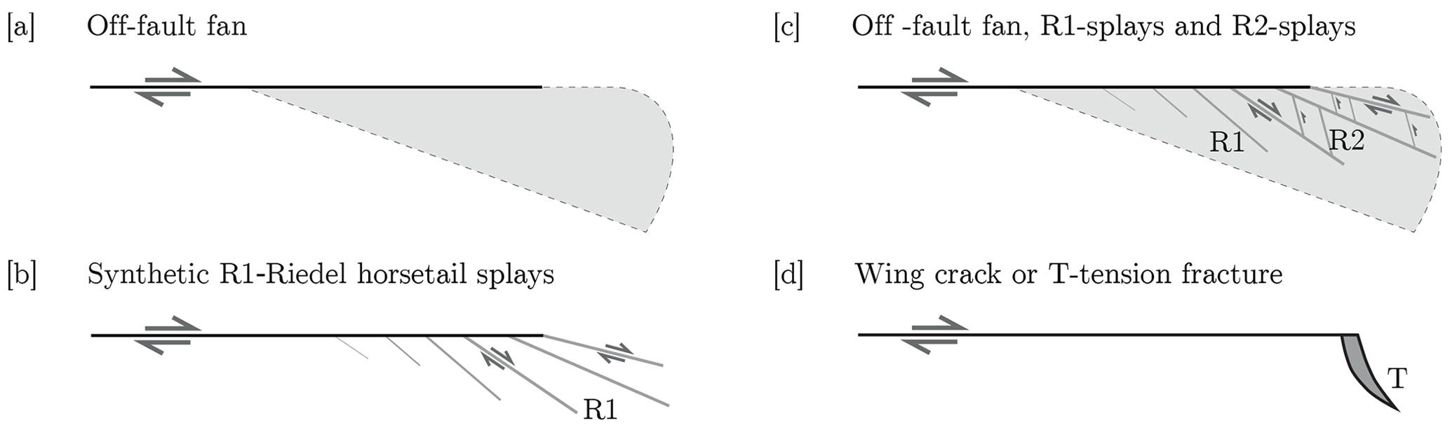
Figure 1Fault structures developing at the tip of a sliding strike-slip fault. Modified from Kim et al. (2004) and combined with schematic interpretations from Faulkner et al. (2011) and Perrin et al. (2016b). R1 is the synthetic Riedel shear fracture, R2 is the antithetic conjugate Riedel shear fracture, and T is the tension fracture or wing crack.
The secondary fault structures altogether constitute the wake of a permanent off-fault damage zone (Scholz et al., 1993; Manighetti et al., 2004; Perrin et al., 2016b), alternatively termed an off-fault fan (Fig. 1a, c). This fan is also present around very well-localized principal slip zones (Shipton et al., 2006). Field observations indicate that the damage fan width scales with accumulated fault displacement (Perrin et al., 2016b, a). At a smaller distance from each fault, an inner damage zone of microfractures also develops, whose width does saturate at a few hundred meters for larger displacements (Mitchell and Faulkner, 2009; Savage and Brodsky, 2011; Ampuero and Mao, 2017). During an earthquake, energy is dissipated in the damage zone over large distances from the fault (Cappa et al., 2014; Ampuero and Mao, 2017). Earthquakes not only operate on the main fault structure but can also propagate on secondary faults (Mitchell and Faulkner, 2009). The damage zone also contributes to long-term deformation. For example, secondary faults in California accommodate up to 43 % of the total fault slip rate of mapped faults taken from the Southern California Earthquake Center Community Fault Model (data from Plesch et al., 2017).
Initial attempts to simulate plastic off-fault deformation in elastodynamic earthquake mechanics models were undertaken by Andrews (1976). The plastic fan width was directly related to the rupture propagation distance (Andrews, 2005; Rice et al., 2005). Factors controlling the extent and distribution of off-fault plasticity during dynamic rupture were analyzed by Templeton and Rice (2008). The effect of plasticity on transitions between different rupture styles was studied, and the prestress angle was shown to have an influence on rupture speed, plastic zone width and the rotation angle of the total seismic moment (Gabriel et al., 2013). A theoretical and numerical study of 3-D rupture with off-fault plasticity revealed how the seismogenic depth of a fault limits the width of the inner damage zone (Ampuero and Mao, 2017). Dynamic earthquake ruptures were shown to propagate along self-chosen paths of a simplified, persistent, branched fault geometry (e.g., Bhat et al., 2004, 2007). Formation of localization in dynamically generated damage zones was linked to branched faults in a micromechanics-based model allowing for the incorporation of crack growth dynamics (Bhat et al., 2012). A recent 2-D dynamic earthquake rupture modeling study nicely shows coseismic off-fault damage during earthquake ruptures at different depths and analyzes its contribution to the overall energy budget (Okubo et al., 2019). Geometrically more complex faults and elastic–plastic off-fault response due to singular events in non-evolving media were studied in a generic case (Fang and Dunham, 2013) and in a realistic fault geometry model of the Landers earthquake (Wollherr et al., 2019). The main limitation of all these modeling studies is that they are restricted to one single earthquake, a fixed and mostly single main fault that is unable to extend, a simplified background stress state represented by a fixed orientation of the principal stress (e.g., Okubo et al., 2019), and an artificial nucleation for numerical convenience (e.g., Gabriel et al., 2013; Okubo et al., 2019). A first attempt to study dynamic branching in self-chosen crack paths was undertaken by Kame and Yamashita (2003). Their study shows crack bifurcation into two branches in homogeneous elastic media. Their modeling approach does not account for visco-elasto-plastic media or recurrent coseismic events interspersed by aseismic interseismic phases. Recent efforts have advanced the timescales of the simulations to model earthquake cycles on strike-slip faults governed by rate and state friction in 2-D anti-plane (vertical cross section) with off-fault plasticity (Erickson et al., 2017). However, 2-D anti-plane approaches cannot model the horizontal propagation of strike-slip faults and their off-fault branches, and models with diffuse plastic deformation cannot simulate localized off-fault branches explicitly. Nor can these dynamic models grow fault branches interseismically.
In this paper we develop a computational model that combines the following features: dynamic off-fault yielding in a visco-elasto-plastic material, long-term evolution of a geometrically complicated fault system, consistent simulation of multiple subsequent earthquakes on the same fault system and the effect of the finite seismogenic–elastic depth. Our method builds upon and extends the recently developed STM-RSF numerical model for seismo-thermomechanical modeling under rate and state friction (van Dinther et al., 2013b; Herrendörfer et al., 2018; Preuss et al., 2019) to, for the first time, simulate cyclic seismic and aseismic fault growth. The STM model was developed in van Dinther et al. (2013a, b) to bridge long geodynamic timescales of fault and lithosphere evolution with short timescales approximating earthquake sequences in a visco-elasto-plastic medium. It was extended to simulate spontaneous off-fault events in van Dinther et al. (2014). Herrendörfer et al. (2018) developed the STM-RSF version to simulate sequences of earthquakes with time steps down to milliseconds using a new invariant rate and state friction (RSF) formulation on predefined, mature faults. Preuss et al. (2019) extended the STM-RSF code to simulate aseismic and seismic fault growth. However, once a fault was formed and ruptured dynamically in a velocity-weakening bulk medium it continued to rupture indefinitely if unhindered by model boundaries.
To accurately simulate cyclic fault growth with off-fault plasticity we extend this STM-RSF framework with three new features. First, we compare four different rate-dependent rheologies in the bulk material. The most realistic one is inspired by laboratory friction experiments and includes a weakening of RSF parameters with plastic strain (e.g., Beeler et al., 1996; Marone and Kilgore, 1993). These rheologies allow us to simulate distributed and localized coseismic off-fault deformation during dynamic rupture propagation spanning all the possibilities presented in Fig. 1. Second, we expand the 2-D framework to 2.5-D using a generalized Elsasser approach (Lehner et al., 1981). Recent work has shown that the thickness of the plate has a direct effect on the width of the inner damage zone, leading to saturation as a function of rupture length (Ampuero and Mao, 2017). The 2.5-D approximation accounts for stresses generated at depth to counteract sudden displacements originating from a crustal earthquake. It allows us to analyze which factors control the width of the damage zone. Third, we introduce a new rate-dependent fault-width formulation to avoid mesh dependency of our simulation results, an issue raised in previous numerical work (e.g., Templeton and Rice, 2008; Bhat et al., 2012). Ultimately, with this new set of models we study the spatiotemporal evolution of an (a)seismically extending preexisting main fault. The application of driving plate velocities at the boundaries of the crustal block results in the concentration of stresses on the fault, which leads to consecutive earthquakes. These sudden dynamic events are interspersed by aseismic periods (interseismic phases). The two processes together shape the long-term structure of the fault system by extending the main fault. The mode of propagation depends on various properties of the host rock. We compare the orientations of the newly developed faults to the predictions of classical Mohr–Coulomb failure theory and distinguish aseismic from seismic growth contributions. Furthermore, we test the role of the optimality of the angle of the preexisting fault in the amount of coseismic off-fault deformation. Various implications of our results are discussed in Sect. 4.
We summarize the main ingredients of the STM-RSF modeling approach in Sect. 2.1 but refer the reader to Herrendörfer et al. (2018) for more details. This description focuses on incorporating three new model ingredients: a 2.5-D approximation (Sect. 2.1), a dynamically adapting fault width during the localization process (Sect. 2.2) and a plastic-strain-dependent bulk rheology behavior as described in the model setup (Sect. 2.3).
2.1 Seismo-mechanical modeling with rate- and state-dependent friction and a 2.5-D approximation
We expand the 2-D STM-RSF framework to 2.5-D using a generalized Elsasser approach introduced by Rice (1980) and Lehner et al. (1981). The 2.5-D model captures the concept that rapid deformation in the elastic–brittle upper crust exerts a shear stress load onto the deeper viscoelastic crustal substrate, which then relaxes slowly and transfers stresses back to the upper crust (Lehner et al., 1981). Assuming, for simplicity, a Maxwell coupling between the upper and lower crust, the shear tractions at their interface are approximated as thickness-averaged stresses (chap. 10 in Rice, 1980). Weng and Ampuero (2019) showed that the energy release rate of dynamic ruptures in a 2.5-D model approximates that of long ruptures with finite seismogenic depth very well in a 3-D model. The 2.5-D simulations thus approximately account for the 3-D effect of a finite rupture depth at the same computational cost as a 2-D simulation.
In 2.5-D we solve for the conservation of mass,
and the conservation of momentum:
where and are coordinate indices, xi and xj represent spatial coordinates, ρ denotes density, is the material time derivative, vi is velocity, and gi is gravity. P is the dynamic total pressure, defined as positive under compression, computed from the mean stress as
The deviatoric stress tensor τij, with , in the crust is given as
with σij being the Cauchy stress tensor and δij the Kronecker delta. They are linked to deviatoric strain rates by the following visco-elasto-plastic constitutive relationship (Gerya and Yuen, 2007):
where G is the shear modulus, denotes the corotational time derivative, η is the effective ductile viscosity in the crust, is the second invariant of the deviatoric plastic strain rate and is the second invariant of the deviatoric stress tensor in 2.5-D. The stresses at depth are averaged over the thickness of the crust T as (Lehner et al., 1981)
where ui represents the displacements averaged over the thickness of the crust, T, and TS is the thickness of the lower crustal substrate with shear modulus GS and viscosity ηS. The geometric factor is designed to match the energy release rate between 2.5-D and 3-D dynamic rupture simulations (Weng and Ampuero, 2019). The medium is compressible, so density and pressure are related by
where K is the bulk modulus. The onset of plastic deformation is defined by the yield criterion:
where with the pore fluid pressure factor , σc is the constant compressive strength that marks the residual strength at P=0 and μeff(RSF) is a variable effective friction parameter that we define based on our continuum RSF formulation. We use a modified Drucker–Prager plastic yield function (Drucker and Prager, 1952) in the form
where
is the local friction coefficient that is widely used and obtained from laboratory experiments, and
is the local cohesion.
The local effective friction parameter μeff(RSF) evolves according to the invariant reformulation of rate- and state-dependent friction for a continuum, introduced by Herrendörfer et al. (2018). This formalism was applied to freely and spontaneously growing seismic and aseismic faults by Preuss et al. (2019) by interpreting how plastic deformation starts to localize and forms a shear band that approximates a fault zone of finite width that can host earthquakes.
Localized bulk deformation and fault slip are related by defining the plastic slip rate Vp as
where W denotes the width of the fault zone in the continuous host rock. We formulate μeff(RSF) as
where a and b are laboratory-based empirical RSF parameters that quantify a direct effect and an evolution effect of friction, respectively, L is the RSF characteristic slip distance, μ0 is a reference friction coefficient at a reference slip velocity V0 (Lapusta and Barbot, 2012), and C is the cohesion as part of the state variable θ (Marone et al., 1992) that evolves according to the aging law:
To solve the governing equations we use an implicit, conservative, finite-difference scheme on a fully staggered grid combined with the marker-in-cell technique (Gerya and Yuen, 2003, 2007). All details of the numerical technique that comprise the STM-RSF code can be found in Herrendörfer et al. (2018).
2.2 Slip-velocity-dependent fault-width formulation
In contrast to previous studies, in which fault width W in the slip-rate formulation of friction was constant (e.g., van Dinther et al., 2013a, b; Herrendörfer et al., 2018; Preuss et al., 2019), we introduce a dynamically adapting W. Deformation localizes to within one to two grid cells in classical applications of plasticity (e.g., Lavier et al., 2000; Buiter et al., 2006; van Dinther et al., 2013a). In models involving a preexisting fault, Herrendörfer et al. (2018) found that setting W=Δx leads to convergence with respect to grid size. However, this choice is not optimal in models involving the spontaneous formation of a fault because it leads to grid-size-dependent fault orientations (on the order of a few degrees) and earthquake onset times (Preuss et al., 2019). This results from the elastic loading phase, in which, for larger grid sizes, the same slip velocity is scaled to a smaller effective plastic strain rate. This yields a higher visco-plastic viscosity and thus higher stresses, resulting in a larger slip velocity. This higher slip velocity, in turn, leads to a faster evolution of state and thus to a faster localization of deformation. The higher stresses additionally induce a higher local friction coefficient in the undeformed matrix, and hence the fault angle becomes larger (Preuss et al., 2019). To prevent this dependence on grid size, we introduce a length scale in the relationship between slip rate and plastic strain rate that incorporates the distributed deformation during the fault localization phase, which may span more than one grid cell.
We propose a new invariant continuum-based RSF formulation, in which the fault width W adapts dynamically as a function of the slip velocity Vp during the strain localization phase. We define a rate-dependent width
and complement it with lower and upper bounds as
The dimensionless scaling parameter K=1 determines the onset of localization. The upper fault-width limit Wmax is defined as the width of inelastic interseismic deformation obtained from fault-parallel GPS and InSAR data. We get a first-order estimate of this quantity by measuring the half-width of the fault-parallel velocity approaching the far-field plate velocity asymptotically. Wmax can vary significantly between ∼2 km (Jolivet et al., 2013) and ∼100 km (Jolivet et al., 2015; Lindsey and Fialko, 2016) in natural faults and depends on the crustal material and thickness, the rate of deformation, and the size of the respective fault zone. Consequently, we set Wmax=20 km as an averaged proxy for the fault width in the interseismic phase. The relation (Eq. 15) can be interpreted as a heuristic fix to the problem of grid-size-dependent localization in continuum models with RSF. We base this fix on the fact that slow crustal movements in the interseismic period lead to distributed deformation (Collettini et al., 2014), e.g., within the Pacific–North American plate boundary, which is very wide in the north, across the San Andreas Fault and the eastern California shear zone segments (Wdowinski et al., 2007). On the other hand, faults show localization of deformation during coseismic periods, sometimes identifiable at large depths by the presence of pseudotachylyte (Sibson, 1977, 1983; Swanson, 1992; Norris and Toy, 2014; Ikari, 2015). Examples of highly localized slip planes are numerous in different rock types and on different scales (e.g., Chester et al., 1993; Chester and Chester, 1998; Sibson, 2003; Smith et al., 2011; Barth et al., 2013; Collettini et al., 2014; Rice, 2017). Also, laboratory experiments reveal that strain is initially distributed across the full thickness of a sheared gouge layer, but after some displacement it localizes to a high-strain principal slip surface (Smith et al., 2015; Ritter et al., 2018a, b). These principal slip surfaces, which seem to be a prerequisite for future earthquake slip, form at subseismic slip velocities (Ikari, 2015). This behavior is affirmed by numerous experimental and microstructural studies that report a fine-grained shear localization zone cut by a discrete principal slip zone during sliding at seismic velocities (e.g., Toro et al., 2004; Brantut et al., 2008; Han et al., 2010; Scuderi et al., 2013; Paola et al., 2015; Pozzi et al., 2018). Alloy in extension and compression shows an analogous sequence of formation of coarse deformation bands followed by shear strain localization, leading to crack formation (Price and Kelly, 1964). A common mode of failure in granular materials involves the same pattern of localization of homogeneous deformation into a narrow zone of intense shear (Jenkins, 1990). In addition, our heuristic fix follows the general tendency for the logarithmic rate dependency of materials, which appears in, e.g., friction as well as porosity and dilatancy (Dieterich, 1981; Logan and Rauenzahn, 1987; Sleep, 1995; Segall and Rice, 1995; Beeler et al., 1996; Chen et al., 2017).
The result of using the new slip-velocity-dependent fault-width formulation is that both the fault angle and the onset times of earthquakes converge with grid size (Appendix A).
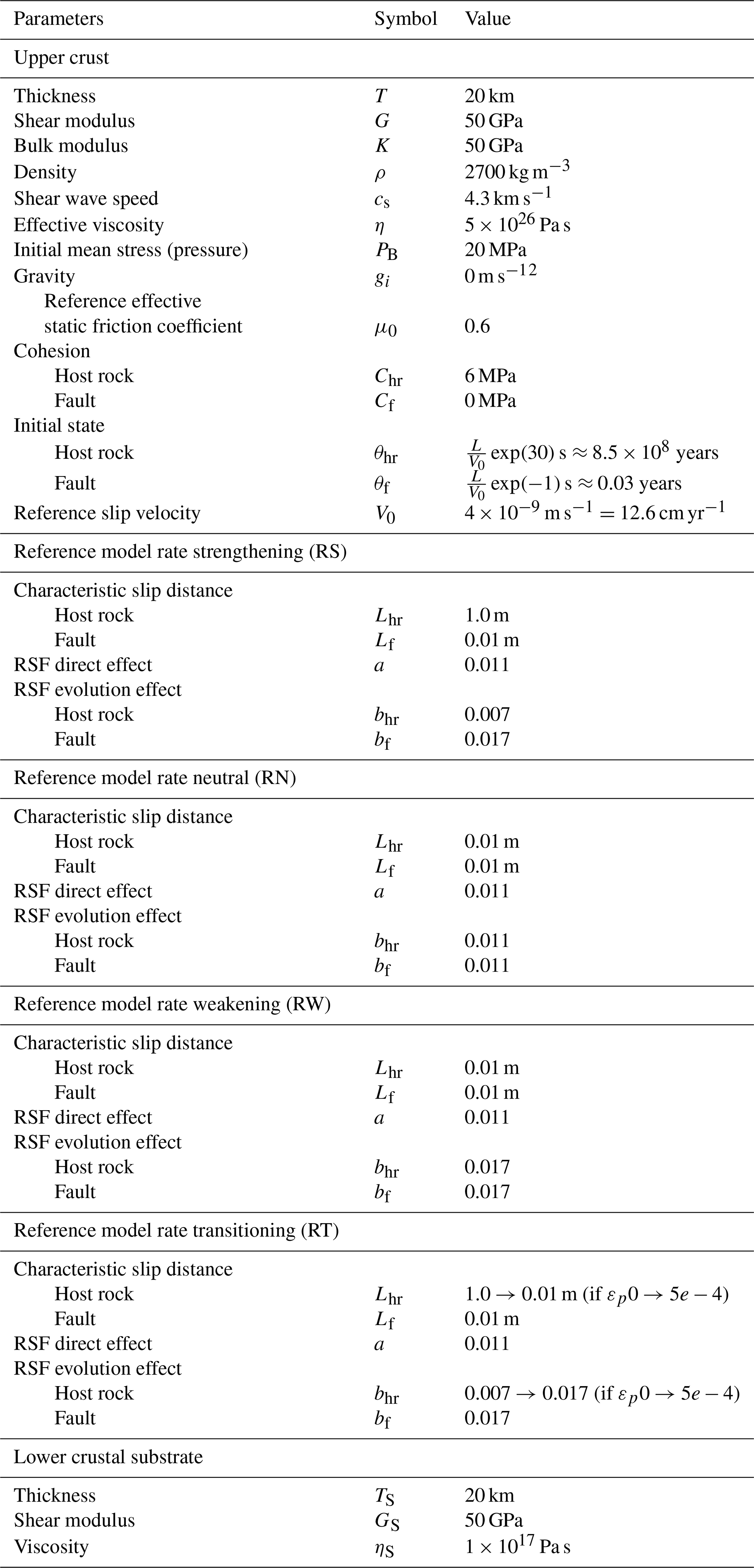
Table 1Rate- and state-dependent friction (RSF) and material parameters of the four 2.5-D reference models.
2.3 Model setup
Our 2.5-D model setup represents a generic case to study the evolution of a fault zone within a plane strain crust of 20 km thickness coupled to an underlying lower crustal layer of 20 km thickness. The model horizontal size is 250 km×150 km. The third dimension is reduced by depth averaging, leading to a 2.5-D model (Sect. 2.1). The initial fault is prescribed as a 120 km long line of lower state θ and zero cohesion C compared to the host rock. It represents the tip of a mature fault in nature and will be the locus of stress concentration, leading to the spontaneous nucleation and propagation of a rupture as a mode II crack. The experimental geometry, together with the Dirichlet vx-velocity boundary conditions applied in opposite directions at the back and front boundaries, represents a dextral strike-slip zone (Fig. 2).

Figure 22.5-D model setup of the dextral in-plane strike-slip simulation: 2-D box of size 250 km×150 km with 501×301 nodes in the x and y direction, respectively (grid resolution of 500 m). Each cell contains 16 markers, resulting in 2 400 000 global mobile markers. Bold black shear arrows indicate the direction of Dirichlet vx-velocity boundary conditions applied in the opposite direction: m s−1. At the left and right boundaries, Neumann boundary conditions for vx are prescribed. Velocity vy is set to zero at all boundaries. The 120 km long fault (in gray) has a lower state θ compared to the host rock. The third (z) dimension is approximated by a depth averaging of upper crustal stresses due to a relaxed lower crustal substrate (Sect. 2.1). A symbolic earthquake rupture occurring on the fault is shown by horizontal x-velocity contours in red and blue at the location of a seismic wave sign. Light green arrows with white contours mark the direction of the principal compressional stresses; the maximum one, σ1, is initially oriented at 45∘. The counteracting effect of the rupture on stresses in the relaxed substrate is shown by the red dashed arrows. The directionality of shear tractions σxz and σyz on the lower surface of the upper crust is represented by black arrows with triangular heads. The quantities ηS and GS and the dimensions T and TS are listed in Table 1.
The maximum compressive stress σ1 is initially oriented at an angle of 45∘ to the imposed shear direction, indicated by the light green arrows in Fig. 2 (e.g., Meyer et al., 2017). Values of the reference model parameters (Table 1) are set largely in accordance with Lapusta et al. (2000), with differences in the choice of V0 and the initial mean stress PB. Following Herrendörfer et al. (2018), we set V0 equal to the loading rate. The background effective pressure PB=20 MPa can be related to the lithostatic pressure and the pore fluid pressure Pf by
Considering a typical value of the pore fluid pressure ratio λ∼0.67, the lithostatic pressure is MPa, which is equivalent to a depth of 2.3 km, representing the upper crust. In Sect. 3.2.1 we simulate at higher and lower pressures that represent higher and lower depths, respectively.
In this study we present four different reference models with varying RSF behavior in the bulk: model RS has rate-strengthening behavior, model RN has rate-neutral behavior, model RW has rate-weakening behavior, and model RT has a transition from rate-strengthening to rate-weakening behavior at increasing plastic strain. We choose to study these different bulk behaviors because in the literature of materials and geology both strain-rate strengthening and strain-rate weakening are reported to be possible and sufficient conditions for localization of deformation (Hobbs et al., 1990). By studying these different bulk behaviors we are able to emphasize their different characteristics. In the first three cases, (a−b) and L are kept constant in the entire model domain. In model RT, (a−b) and L decrease with plastic strain (Table 1), motivated by laboratory observations (Beeler et al., 1996; Scuderi et al., 2017; Marone and Kilgore, 1993).
In the first part of this section we present and compare the results of the four models to understand the effects of a rate-sensitive bulk rheology on off-fault deformation and fault growth. We then focus on two reference models to further investigate factors influencing the off-fault fan width and the role of viscoelastic lower crust relaxation in short-term and long-term off-fault deformation (Sect. 3.2). In Sect. 3.3 we study the role of the angle of the predefined fault in off-fault deformation. Finally, we analyze the formation of localized secondary branches (Sect. 3.4).
3.1 Role of rate-dependent bulk rheology on off-fault deformation and fault growth
The initial elastic loading phase takes 325.5 years in all four reference models. In this initial stage stresses start to localize on the predefined fault and its slip velocity increases exponentially (Fig. 3b). About 5.5 years after the slip velocity reaches the plate velocity, an earthquake nucleates on the fault at x=0 km and propagates eastwards along the fault. During the earthquake, the on-fault slip rate Vp rises to seismic slip velocities, as defined by the typical dynamic scale Vseis introduced by Rubin and Ampuero (2005) (Fig. 3b). The generation of coseismic off-fault plastic deformation is a general feature of our models (Fig. 3a). It occurs on the extensional side of the fault, which is favored over the compressional side when the maximum principal compressional stress direction is (Kame et al., 2003). The off-fault plastic zone grows continuously in a fan-like manner, but eventually its thickness (fault-normal size) saturates at a value of ∼8 km and at a rupture distance of ∼80 km. Concurrently, the slip velocity reaches a maximum at Vp=1.1 m s−1. The maximum width of the off-fault fan Hmax and the onset of saturation are affected by various parameters investigated in Sect. 3.2.1.
Besides these general similarities among the four reference models, we note two main differences. First, the plastic zones off the main fault have distinct characteristics. A fan of diffuse deformation occurs in models RS and RT, while localized deformation on secondary faults occurs in models RN and RW. Thus, the type of plastic off-fault yielding depends on the properties of the bulk rheology. Only a rate-neutral or rate-weakening material in which L is comparatively low (0.01 m) allows for fault localization in the off-fault material. Each of the secondary fault branches is formed by individual secondary dynamic ruptures during the first main fault rupture. This localization behavior will be addressed further in Sect. 3.4.
The second main difference is that only model RT hosts a sequence of several earthquakes. In the other three models the entire new fault geometry forms during a single earthquake, an aftershock, and the subsequent post-seismic and interseismic phases. Before more seismic events can nucleate, the main fault has already extended by aseismic growth toward a model boundary and the simulation is stopped to prevent boundary effects. The models with constant rate sensitivity (models RS, RN and RW) have fast fault growth rates of up to 77 km yr−1 that are much faster than in model RT. Despite this major difference, all reference models have in common that fault growth during the earthquakes contributes only a small portion to the total formed fault length FL (Fig. 3b).
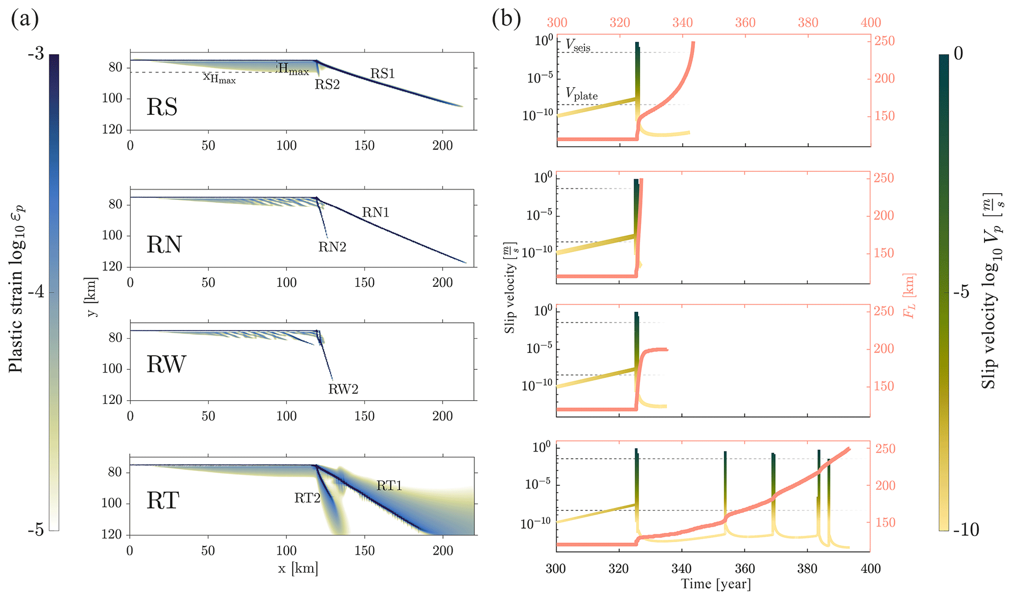
Figure 3Summary of four different right-lateral reference models. (a) Simulation results in the form of a plastic strain pattern. RS: rate strengthening, RN: rate neutral, RW: rate weakening, RT: transition from RS to RW. R*1 indicates a Riedel fault (lower strike angle), and R*2 refers to the conjugate Riedel fault (R′) with a higher strike angle compared to the R1 Riedel shear. The snapshots in (a) are chosen to have approximately the same deformation stage with regard to fault length R*1. Model RW constitutes an exception as RW1 remains very short (1.8 km; see the main text). (b) Temporal evolution of the plastic slip velocity Vp inside the fault at (100, 75 km) until the end of the simulation. The seismic threshold velocity is indicated as Vseis. The red line shows the fault length FL over time.
In the following analysis we mainly focus on models RW and RT because the off-fault characteristics of models RW and RN are similar, and those of models RT and RS. Furthermore, RW and RT represent the two cases of dominant higher-angle and lower-angle continuing faults, respectively. In that way, RW and RT are the most diverse end-member cases of the four reference models. At the same, time model RT is the most realistic model with successive earthquakes, distributed deformation and localized fault growth. Model RW, on the other hand, allows for strong off-fault localization and tends towards irregular fault patterns with unevenly spaced secondary fault branches.
3.1.1 Temporal and geometrical evolution of fault growth
As the main fault propagates beyond the tip of the predefined fault, all four reference models form two new faults with two orientations. A “higher-angle fault” forms with a high angle compared to the strike of the predefined fault. It is an antithetic conjugate Riedel shear fault and is termed R*2, wherein “*” stands for the different reference models. A “lower-angle fault” forms with a lower strike angle and is a synthetic Riedel shear fracture termed R*1 hereafter. Detailed analysis of model RT reveals that these two faults are formed because the main fault rupture induces two stress lobes on the extensional side of the fault. These zones were studied by Poliakov et al. (2002), who termed them “secondary faulting area”. These areas also evoke lobe-like anomalies of the dynamic friction value. Later on, the frontal lobe is responsible for the formation of RT1, and the back lobe forms the conjugate fault RT2 (Fig. 4a, b). This behavior of model RT is representative for all four reference models. We confirm that both faults form according to the Mohr–Coulomb failure criterion at either the Coulomb fault angle (R1 fault) or the conjugate angle (R2 fault). These angles α are
where φ denotes the internal angle of friction, related to the local friction coefficient μ(RSF) that we call μl for simplicity in the following, by μl=tan φ. The angle α spans between the maximum principal compressional stress direction σ1 and β, the angle of the newly forming fault, such that (Fig. 4c). The reference angle is the horizontal shear direction. The compressive state of stress in our simulation limits α: and (conjugate). We take the average of σ1 and μl to compute the resulting α at three different instants: (1) 5 s before fault propagation, (2) 1 min after the initiation of the first fault propagation and (3) 25 years after the initial fault propagation (Fig. 4d, symbols □, ∘, ⋄, respectively). These data reveal that the local dynamic conditions in the proximity of faults determine the angles of the faults RT1 and RT2, which was previously reported for an isolated growing fault (Preuss et al., 2019). Additionally, they approach the theoretical angle α and converge on it with advancing time (Fig. 4d). This behavior indicates that the absolute fault angles β of RT1 and RT2 are predictable, even before the faults have formed. As soon as the two lobes are formed by elevated stresses near the rupture front, i.e., approximately 10 s after the earthquake nucleation, they have the potential to determine the angle of the R fault and the R2 conjugate (Fig. 4e). Both RT1 and RT2 exhibit a lower final strike angle than their predictions during the dynamic phase. This is justified by the fact that seismically growing faults have a higher strike angle than aseismically forming faults (Preuss et al., 2019). Thus, the seismically initiated fault decreases in strike angle as soon as the slip velocity transitions to the non-seismic range. This happens as the rupture hits the undeformed host rock. Indeed, at the end of the first earthquake the fault extends in a pure seismic mode, and the angle of the new fault is greater than in the following interseismic phase after the earthquake. Hence, both RT1 and RT2 flatten in the 0.3 years right after the first earthquake and before the aftershock. This behavior is visible in the online videos (link to video RT, 116 Mb, https://www.research-collection.ethz.ch/bitstream/handle/20.500.11850/397242/Video_Model_RT_reduced.mov?sequence=22&isAllowed=y, last access: 28 May 2020; RS, 41 Mb, https://www.research-collection.ethz.ch/bitstream/handle/20.500.11850/397242/Video_Model_RS_reduced.mov?sequence=23&isAllowed=y, last access: 28 May 2020; RN, 41 Mb, https://www.research-collection.ethz.ch/bitstream/handle/20.500.11850/397242/Video_Model_RN_reduced.mov?sequence=24&isAllowed=y, last access: 28 May 2020; RW, 68 Mb, https://www.research-collection.ethz.ch/bitstream/handle/20.500.11850/397242/Video_Model_RW_reduced.mov?sequence=25&isAllowed=y, last access: 28 May 2020) just after the first earthquake, in Fig. 4b and in all four reference model snapshots (Fig. 3a).
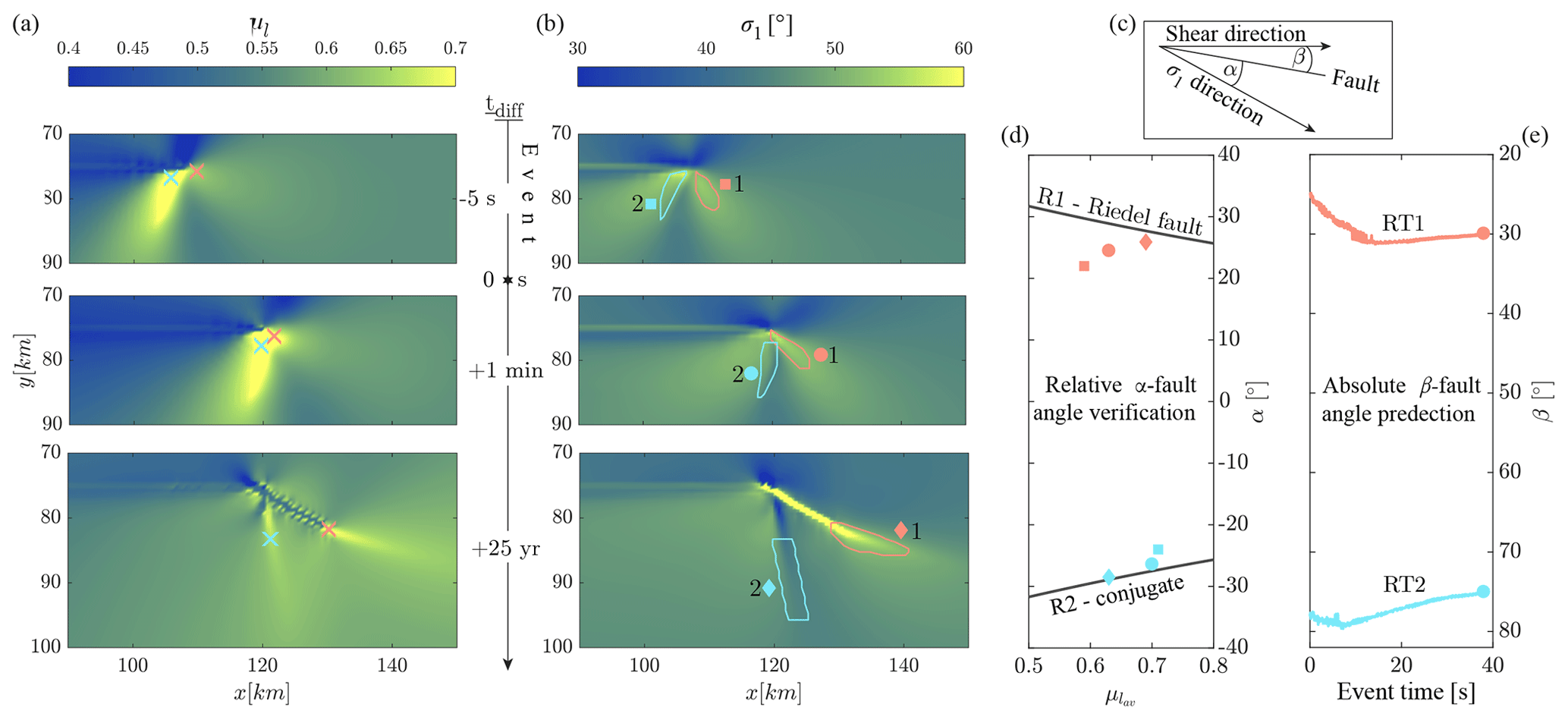
Figure 4Evolution of the local friction coefficient and stress orientation of model RT over time and the prediction of the absolute fault angle. The three different times are (1) 5 s before fault propagation (symbol □), (2) 1 min after the initiation of the first fault propagation (symbol ∘) and (3) 25 years after the initial fault propagation (symbol ⋄). Red represents the Coulomb angle of R1, and turquoise refers to the conjugate fault R2. (a) Snapshot zooms of the local friction distribution μl at different times. Crosses indicate the location of the two maxima of μl at the rupture tip or at the tip of the newly formed fault. (b) Snapshot zooms of the distribution of the maximum compressive stress orientation σ1 at different times. Red and turquoise polygons indicate the locations around the frictional maxima inside the two stress lobes where μl and σ1 are sampled and averaged according to 2 standard deviations of the mean (95th percentile). (c) Schematic geometrical relation in physical space between horizontal shear direction, σ1 direction and forming fault. β represents the absolute fault angle, and α is the angle between the fault and the σ1 direction such that . (d) Relation between averaged local friction coefficient and fault angle α1,2, which is obtained from the average σ1 directions for the three different instants shown in (a) and (b) for R1 and R2, respectively. The values from the frontal lobe result in the data converging on the R1 Riedel angle α1, and the data from the back lobe converge on the R2 conjugate α2. Black lines indicate the theoretical angle given by Eq. (18). (e) Prediction of the absolute fault angles β1,2 for both RT1 and RT2 from sampling averages of μl and σ1 during the entire first dynamic earthquake.
The different reference models favor either of the two fault angle types or develop them jointly. The smaller the initial L and a−b in the bulk material, i.e., with more weakening, the higher the tendency to favor the high-angle conjugate fault (Fig. 3). This behavior is evident if one compares models RS and RW. An intermediate situation occurs in models RN and RT when both fault types are well developed and evolve in an approximately equal manner. A second result of lower initial L and a−b is the greater generated fault length in response to the primary seismic event: FL=12.3 km (RW2), 11.3 km (RN2), 8.3 km (RS2) and 7.4 km (RT2). Hence, an earthquake can extend a fault farther in a rate-weakening material than in a rate-strengthening material, and the rate transition case produces the shortest seismic growth. The aseismic fault growth rate in a rate-neutral material is higher than in a rate-strengthening material (Fig. 3b). Most likely it is even higher in a rate-weakening material, but a comparison is impeded because model RW favors a different fault growth path.
In the following we describe the evolution of the R1 fault and the conjugate R2 in detail for the four individual model cases (link to video RT, 116 Mb, https://www.research-collection.ethz.ch/bitstream/handle/20.500.11850/397242/Video_Model_RT_reduced.mov?sequence=22&isAllowed=y, last access: 28 May 2020; RS, 41 Mb, https://www.research-collection.ethz.ch/bitstream/handle/20.500.11850/397242/Video_Model_RS_reduced.mov?sequence=23&isAllowed=y, last access: 28 May 2020; RN, 41 Mb, https://www.research-collection.ethz.ch/bitstream/handle/20.500.11850/397242/Video_Model_RN_reduced.mov?sequence=24&isAllowed=y, last access: 28 May 2020; RW, 68 Mb, https://www.research-collection.ethz.ch/bitstream/handle/20.500.11850/397242/Video_Model_RW_reduced.mov?sequence=25&isAllowed=y, last access: 28 May 2020). In the RS model with pure rate-strengthening behavior, RS1 and RS2 are created simultaneously as the seismic rupture penetrates into the bulk, and they are equally long. Then, the left-lateral RS2 transitions into a passive state, becomes abandoned and stops growing, while the right-lateral branch RS1 extends aseismically. We record no pronounced off-fault deformation for either RS1 or RS2. They are rather localized fault strands that are wider than the newly formed faults in the other models, however.
In the rate-neutral model the propagating rupture excites several equidistant secondary splay faults that form under the same Coulomb angle (R1) and saturate at x∼80 km such that they are 16.5 km long as a maximum. As the main rupture and the secondary ruptures penetrate into the bulk, two of the secondary splay faults that were triggered by the dynamic main fault rupture continue to grow by ∼5 km at a constant Coulomb angle and are then abandoned. Simultaneously, the main rupture initiates RN1 and RN2 under the respective Coulomb angles of the Riedel shear and the conjugate shear. Right after the earthquake, the left-lateral RN2 is ∼4 times longer than RN1. However, right-lateral RN1 is increasingly favored as both fault branches extend in an aseismic manner and RN1 finally becomes the main extension of the predefined fault. The aseismic phase in which RN1 extends by 130 km and grows towards the right boundary lasts for 1.2 years.
In the rate-weakening model RW, the secondary splay faults form earlier than in model RN and are more localized and partly non-equidistant. Particularly apparent is a secondary splay at x∼105 km that is highly localized and causes a stress shadow on its compressional side, leading to a splay gap. It thus prevents an equidistant spacing of the secondary splays and changes the angles of the subsequent forming splays. We investigate this behavior in Sect. 3.4. As the secondary splays propagate into the bulk at the fault tip they generate approximately 7 km of new fault surface under the conjugate angle of fault RW2, which they are flanking. Subsequently, the secondary faults and the conjugate RW2 merge. In contrast to models RS and RN, model RW reveals a very weakly localized and short incipient fault RW1 (1.8 km). This fault stops growing because the stresses on the compressional side of the compound of secondary branches and the sinistral conjugate RW2 are dominant and limit the extensional side stresses of short RW1. Thus, RW1 remains short and abandoned after the earthquake until the simulation stops such that the sinistral RW2 constitutes the unique extension of the main fault. The simulation RW stops as branch RW2 approaches the lower y boundary at a higher angle. Consequently, the maximum fault length FL is shorter than in the other models.
The off-fault deformation pattern in the rate transition model is composed of similar features as model RS. The two branches RT1 and RT2 form as the main fault rupture penetrates into the undeformed bulk. The fault evolution in model RT spans several earthquake cycles (Fig. 5). Both branches RT1 and RT2 are well developed like in the model RN. However, in the long term branch RT1 grows faster than RT2 during both aseismic and seismic fault growth stages. It is noticeable that the incipient faults in model RT are surrounded by a wide fan of plastic strain that is absent in the other reference models. This fan arises because both RT1 and RT2 host seismic ruptures in contrast to the newly evolving faults in the other reference models. Thus, a plastic fan like the fans next to the predefined fault can grow. Additionally, more strain is accumulated due to a slower fault growth rate (Fig. 3), which prolongs the model run time compared to the other models and facilitates the formation of distributed strain zones. Strikingly, the fan of fault RT1 is on the compressional side, which is due to the increased angle of RT1 relative to the predefined fault where the fan is on the extensional side. Hence, the angle between RT1 and σ1 is smaller than 45∘, which implies yielding on the compressional side of the fault. In contrast to the three other reference models, faults RT1 and RT2 exhibit notable changes in the absolute fault angle β. These bends are ascribed to the difference between lower-angle aseismic and higher-angle seismic fault growth, respectively (Preuss et al., 2019). The repeated sequences of seismic growth increase the overall angle of RT1 compared to RS1 and RN1. Nevertheless, the overall growth contribution in model RT is dominated by aseismic growth. This is clearly visible in Fig. 5 where the aseismic growth increments are opposed to the seismic ones. Seismic fault growth is mainly limited to the first earthquake during which the off-fault damage and the fault branches RT1 and RT2 are created. In the subsequent evolution only marginal portions of fault propagation are ascribed to coseismic events. This seismic contribution is accumulated at the outer edges of the interseismically deformed regions (Fig. 5). The reasons for and implications of these findings are discussed in Sect. 4. Additionally, faults RT1 and RT2 interact with each other. Fault RT2 starts to bend towards RT1 at 360 years. This behavior is not recorded in the other reference models. A seismically initiated connection between RT1 and RT2 at x=130 km that starts at 355 years is also visible.
In summary, the strike angle of the formed faults increases from rate-strengthening to rate-neutral to rate-weakening material. The case of a transition from RS to RW describes a more complex case with intermittent aseismic and seismic growth, fault bends, fault interaction and additional off-fault deformation. In addition, the degree of new fault localization is highest in model RW and follows the order RW, RN, RT and RS.
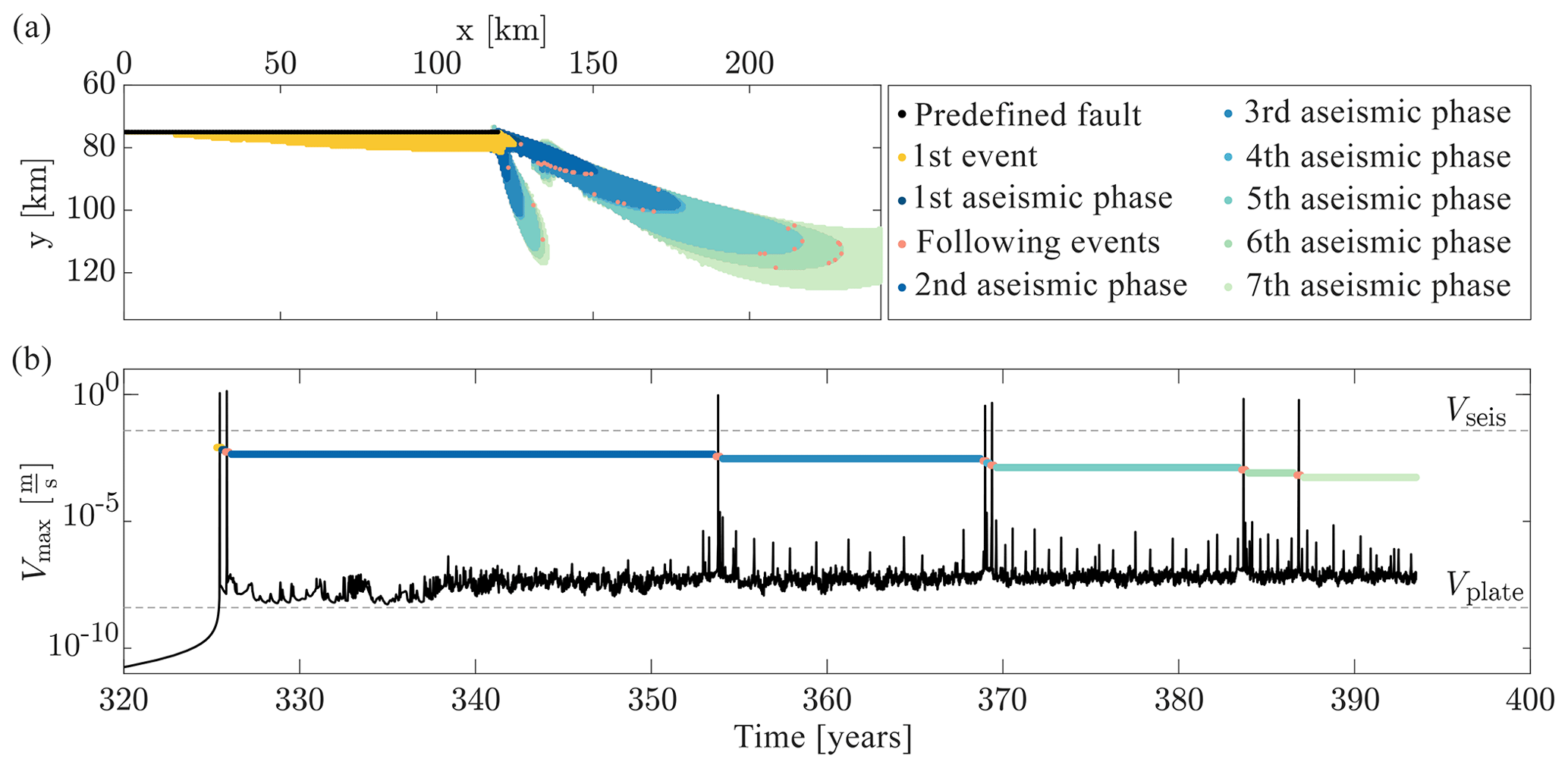
Figure 5Temporal and spatial evolution of model RT with indications of aseismic and seismic fault growth stages in color. (a) Accumulated plastic strain exceeding for different growth stages. (b) Logarithm of the global maximum slip velocity log(Vmax). A video of the simulation can be found in the Video supplement (video model RT, 116 Mb, https://www.research-collection.ethz.ch/bitstream/handle/20.500.11850/397242/Video_Model_RT_reduced.mov?sequence=22&isAllowed=y, last access: 28 May 2020).
3.2 Role of a viscoelastic substrate on off-fault deformation
In this section we first analyze the properties of the saturating plastic off-fault fan and study the determining parameters for this saturation. Secondly, we study the long-term effects of the relaxed viscoelastic substrate on the growth of the splay fault fan.
3.2.1 Off-fault fan and saturation
In all four reference models the plastic off-fault fan reaches a maximal width Hmax at distances over x∼80 km. The onset distance of the saturation does not depend on the bulk rheology. However, Hmax varies from 8.7 km in model RS, to 8.2 km in model RT, to 6.4 km in model RN, to 6.2 km in model RW. In Fig. 6a we show that the slip during the first earthquake saturates; i.e., the rupture develops a flat slip profile. The reason for this behavior is the transition from a crack-like to a pulse-like rupture, which can be seen in the steep tapering-off of the slip velocity (a healing front) in Fig. 6b when the rupture front reaches a distance x∼80 km. This transition to a steady pulse-like rupture results from the finite seismogenic depth. In 3-D rupture models, a healing front emerges when the rupture front reaches the bottom of the seismogenic zone and then travels back to the surface, turning the initial crack-like rupture into a pulse. This interpretation of the saturation of the plastic zone thickness, based on dynamic fracture mechanics and 3-D simulations, was first proposed by Ampuero and Mao (2017). In our 2.5-D approach we do not model the actual rupture front or the healing front at depth. However, the counteracting response of the viscoelastic substrate in the conservation equation of momentum (Eq. 2) captures the effect of stress transfer from depth to the surface. The thickness TS of the lower crustal substrate can be set arbitrarily large and is irrelevant for the model outcome.

Figure 6Accumulated plastic slip and slip velocity during the first earthquake on the main fault plotted in 5 s intervals.
We investigate the impact of crustal thickness T, initial background pressure P, initial bulk host rock state variable θhr and (a−b) on the maximum plastic fan width Hmax for model RT. In our simulation the fan width increases proportionally to the crustal thickness T (Fig. 7a). The onset distance of the saturation is also proportional to T (Fig. 7e). Both characteristics are due to the 2.5-D effect of our simulation. In essence, this T-Hmax relation agrees with the simulation data of Ampuero and Mao (2017, inset of Fig. 13.5 therein). However, our simulation results coincide better with the theoretically determined linear relation between Hmax and T at large T than with the nonlinear trend in the 3-D simulation (Ampuero and Mao, 2017). This is due to a small ratio (nucleation size∕seismogenic depth =0.5) in our simulations, which favors a faster convergence of the curve to the linear trend. Furthermore, the different values of H between the two studies are due to different plastic strain cutoff levels used in the definition of H.
We additionally vary the initial background pressure P from 10 to 40 MPa in steps of 10 MPa and find that the maximum fan width converges to Hmax∼8.5 km, which is 0.3 km wider than Hmax of the reference model RT (Fig. 7b). This implies that Hmax is less sensitive to variations in lithostatic pressure with depth than to the crack-to-pulse-like rupture transition induced by the depth of the seismogenic zone. Our result is consistent with the theory of Ampuero and Mao (2017, their Eq. 13), who found that the maximum fan width is independent of normal stress. A reduction and increase in the initial host rock state variable θhr reveals that the value corresponding to the reference model results in the greatest fan width, while higher and lower state values lead to a reduction of Hmax (Fig. 7c). A change in (a−b) from 0.001 to 0.01 shows that the fan width Hmax converges to a value of 6.4 km for decreasing (a−b), which corresponds to the fan width of the rate-neutral model in which bulk (Fig. 7d). However, since bulk (a−b) is positive in model RT that we analyze here, no localization is reported in contrast to model RN or model RW. A maximum in the relation is reached for with Hmax=10 km. If (a−b) is increased above 0.006 the fan width drops to values below 4 km. This is due to a factor of 2 decrease in the slip velocity (Fig. 7f). Although seems to be anticorrelated with Hmax, which is particularly observable for the crustal thickness and pressure model variations, it has an impact on the fan width in the case of higher (a−b).
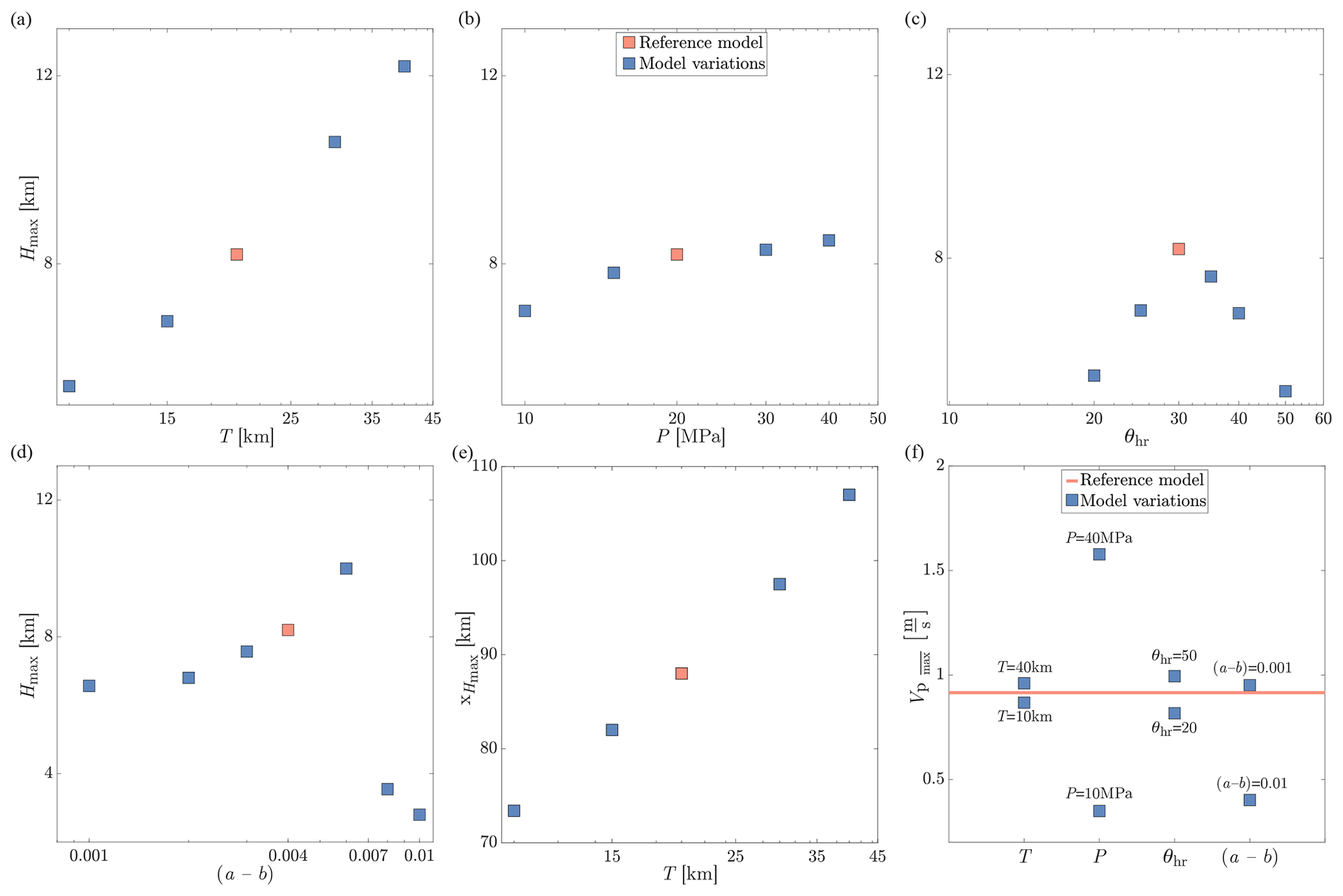
Figure 7Impact of various parameters on the maximum plastic fan width Hmax: (a) crustal thickness T; (b) initial background pressure P; (c) initial bulk host rock state variable θhr; and (d) (a−b). (e) Relation between the onset of the saturation and T. (f) Average slip velocity during the first earthquake as a function of the highest and lowest parameter of each of the four model variations (T, P, θhr, (a−b)).
3.3 Role of the predefined fault angle in off-fault deformation
In Sect. 3.1 and 3.2.1 we demonstrated that the plastic strain produced during the first earthquake reaches similar values for all four reference models. In the presence of localized deformation (models RN and RW) the splay faults form at a greater angle than the predefined main fault. Thus, the optimal angle of a newly forming fault in a dynamically elevated stress field does not coincide with the predefined fault strike. We suppose that the majority of the off-fault strain in these models is due to a “misalignment” of the predefined fault together with the dynamic reorientation of stresses. In order to prove this supposition we design a model with an optimally oriented fault in which the predefined fault strike is at 15∘ to the horizontal shear direction. This is the optimal strike angle, which we obtain by inserting the static friction coefficient μ0=0.6 in Eq. (18). The parameters of the model with an optimally oriented fault are based on model RT. In Fig. 8 we compare the amount of plastic off-fault energy between model RT and the model with an optimally oriented fault. While the reference model RT reaches typical plastic energy values and a typical ratio of on-fault to dissipated off-fault plastic energy (e.g., similar to Okubo et al., 2019), these values for the optimally oriented fault model are substantially lower. In fact, the latter model exhibits almost no off-fault deformation (Fig. 8a), and the amount of plastic energy dissipated to the off-fault material is only 0.2 % (Fig. 8c). This means that the different strike angle of the optimally oriented fault model reduces the magnitude of the off-fault stresses and thus the reach of off-fault deformation. The minor off-fault deformation starting at x≈90 km is due to the dynamic reorientation of stresses, which leaves the preexisting fault slightly misaligned with the dynamic stress field at high slip velocities.
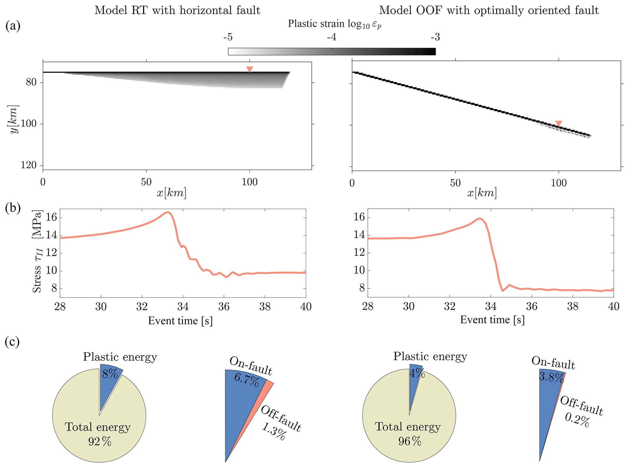
Figure 8Comparison of plastic off-fault strain and energy between model RT and OOF (optimally oriented fault model). (a) Accumulated plastic off-fault strain for both models in grayscale during the first earthquake. Red triangles indicate the sample location of the stress data plotted in (b). Panel (c) shows the ratio of the plastic energy to the total energy in percentage. The plastic energy is subdivided into an on-fault (blue) and an off-fault (red) part.
In Fig. 8b we compare the dynamic stress drop between model RT (3.9 MPa) and the optimally oriented fault model (5.8 MPa). The difference of 1.9 MPa reveals that more energy is concentrated on the predefined fault in the optimally oriented fault model. Additionally, the process of the stress drop is 3.8 s faster than in model RT. We can note that this difference cannot be explained by the theoretical relation in Ampuero and Mao (2017, Eq. 13), in which Hmax∕W is proportional to the ratio of stress drop to strength drop squared. This points to opportunities to refine that theory. In summary, a fault at an optimal angle in the interseismic sense results in a much smaller off-fault plastic yielding during earthquakes. However, due to dynamic reorientations of the fault-near stress field, minor off-fault yielding still occurs.
3.4 Role of higher pressure and a thicker crust on secondary off-fault localization and main fault replacement
In order to increase the strong off-fault localization of reference model RW, with its propensity towards irregular fault patterns and unevenly spaced secondary fault branches, we increase the initial background pressure PB of model RW by a factor of 2 (to 40 MPa). Additionally, we increase the crustal thickness T by a factor of 2, to 40 km, which is a typical value for continental crust and furthermore enhances the extent of off-fault plasticity (Sect. 3.2.1). This model is called HPT. The rate-weakening behavior of the bulk is kept as in model RW to facilitate fault localization. The primary earthquake in model HPT occurs after 656.3 years, which approximately corresponds to twice the event time in model RW. The time lag is caused by the doubled PB and the thicker crust. As the rupture propagates along the predefined main fault, secondary ruptures create localized secondary splay fault branches like in model RW. However, in contrast to model RW, the splays are sharply localized as soon as the off-fault deformation occurs (Fig. 9b). The main fault rupture induces four dynamically rupturing secondary Riedel splays (HPT1, HPT01, HPT001 and HPT0001) under the Coulomb angle. In turn, these splays induce some tertiary ruptures. Each of the dynamically created incipient faults has an extensional and a compressional side, like the main fault. Interestingly, the secondary splays in model HPT do not saturate in contrast to model RW, in which an upper-bound Hmax exists. This is caused by the higher energies of the individual ruptures due to the higher initial background pressure. Hence, this is an indication that the counteracting stresses at the base of the crust are too small to limit the extent of splay faulting in this setting. This behavior is particularly visible for the outermost branch HPT0001, which is the most free to grow and barely interacts with other ruptures as it diverges from the predefined fault. Besides the four Riedel faults, model HPT additionally produces high-angle secondary conjugate faults. This happens even before the main fault rupture penetrates into the bulk at the tip of the predefined fault (fault strands HPT2, HPT02 and HPT002). Some of these conjugate faults extend to connect the main fault with the secondary splays and then stop growing when they intersect with the next fault strand (Fig. 9c). The resulting fault pattern has similarities to fault structures observed in nature and their schematic interpretations (compare to Fig. 1). Another effect of higher PB and thicker T is that the lateral spacing between the separate branches increases such that they become individual independent fault strands. Concurrently, these fault strands can interact with each other due to an interference of the individual local stress fields with the ones of the surrounding dynamic ruptures. This leads to irregularities in splay spacing, splay bending and abandoning of splays. It follows that a higher background pressure increases the degree of localization of the splays and affects the spacing between the splays. Additionally, the complexity in the localized off-fault deformation is increased and the combination with a higher crustal thickness enhances the spatial reach of the off-fault splays. The latter is facilitated by the rate-weakening bulk.
In the following we analyze several indications of fault and rupture interactions due to stress changes that are typically ignored in seismic cycle models. They include (1) rupture arrest when two subparallel ruptures get too close to one another. This can be observed for fault HPT001, which stops growing because the stresses on the extensional side of the subsequently forming branch HPT01 increase, become dominant and limit the compressional side stresses of HPT001. As a consequence, only extensional stresses remain at the tip of HPT001 such that the fault becomes thinner on its compressional side (Fig. 9c, b). This leads to (2) a stop in fault growth and fault abandoning. Further, fault bending (3) is observed as fault HPT02 approaches HPT0001, and the former starts to bend due to local interactions of stresses. After bending, both faults intersect (4), which causes HPT02 to terminate (5). All together, this behavior is clearly visible in the video of the HPT simulation, 19 Mb, (https://www.research-collection.ethz.ch/bitstream/handle/20.500.11850/397242/Video_Model_HPT.mov?sequence=6&isAllowed=n, last access: 28 May 2020). Consequently, new interjacent branches can stop if their extensional side stress field interacts with the compressional side stress field of another rupture. This is the case when the branches of two subparallel ruptures get close to one another. In this process, the fault on the extensional side is likely to continue extending. This line of reasoning applies for a dextral fault system and is reasonable since the evolving fault structure as a total has an extensional character, which means that an extensional stress state is predominant and the extensional fault's side is favored.
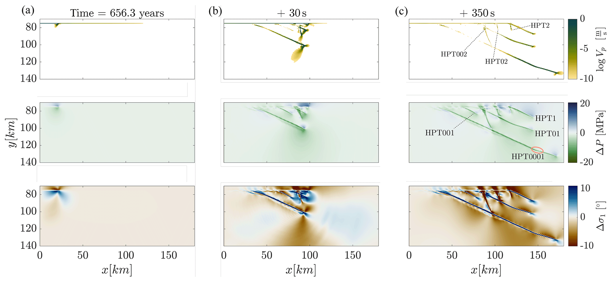
Figure 9Model HPT with higher background pressure (PB=40 MPa) and increased crustal thickness (T=40 km). Plotted are the logarithm of the slip velocity Vp, the pressure difference ΔP between initial background pressure PB and dynamic pressure P, and the dynamic change in σ1 orientation Δσ1 for three different instants in panels (a), (b) and (c), respectively. Different fault branch names are indicated in (c). The red circle in (c) marks the bend of branch HPT0001 due to an aseismic transition phase between two successive earthquakes.
The main fault rupture forms a Riedel fault HPT1 and a conjugate HPT2 like in model RW. These two faults and the secondary branch HPT01 grow until the event slip velocity drops to m s−1 after a duration of 330 s. Then, they stop growing and only the outermost splay HPT0001 continues to grow as the slip velocity again rises to the seismic range. The drop in slip velocity leads to a fault bend (red circle in Fig. 9c). Since the outermost fault is the only active fault at the end of the simulation we infer that during the evolution of the fault network HPT a main fault change occurred. Hence, the branch HPT0001 is most favorably oriented with the local and far-field stresses and replaces the predefined straight main fault. We refer to this dynamic process as a main fault replacement.
Our results suggest that all four reference models have predominantly aseismically growing faults. A bulk rheology with constant rate sensitivity favors faster fault growth. In contrast, the heterogeneities introduced by a weakening of the RSF parameters L and b slow down the faulting process due to the absorption of energy by the weakening mechanism. As a consequence, the faults in the model RT that transition from rate strengthening to rate weakening can extend in alternating seismic and aseismic growth periods. Only if the region ahead of the fault tip has experienced distinct plastic strain and L and b are altered to create a rate-weakening fault earthquakes can propagate there. Otherwise, dynamic rupturing is hindered in the intact bulk, where L is still high and b is still low with rate strengthening. This contrast of large L and low b in the bulk rock results in intermittent seismic and aseismic growth sequences. We think this behavior reflects the natural growth of crustal faults better than constant values of L and b, which lead to rapid fault propagation after singular earthquakes. Furthermore, the evolution of L and b with strain was observed in laboratory studies (e.g., Beeler et al., 1996; Scuderi et al., 2017; Marone and Kilgore, 1993). The differences between the two end-member bulk rheologies have major implications for the dynamics and geometry of fault evolution, which are discussed in this section.
4.1 Riedel shear splays
The concept of work minimization states that new faulting starts when the active fault has become suboptimal in the Coulomb sense and inefficient, with sufficiently high amounts of strain transferred into the surrounding rock (e.g., Cooke and Murphy, 2004; Cooke and Madden, 2014). In fact, natural faults are often unfavorably oriented with respect to remotely acting stresses (e.g., Faulkner et al., 2006). In this case, new secondary faults form at acute Coulomb angles to a primary fault (Scholz et al., 2010). Several studies linked Riedel shears and Coulomb shears (e.g., Tchalenko, 1970). In all our reference models a dynamically formed Riedel fault R1 and a conjugate R2 (R′) emerge at the fault tip. In the rate-weakening and rate-neutral models, Riedel faults dynamically initiate off-fault and grow during the first earthquake, which indicates that the seed fault was not optimally oriented relative to the local dynamic stresses (Fig. 4, discussed in Sect. 4.4).
Interestingly, most of the dynamically generated Riedel faults are abandoned after they form. An exception is the Riedel fault at x=105 km in model RW, which was generated during the first event and grew aseismically 0.35 years later (see video RW, 68 Mb, https://www.research-collection.ethz.ch/bitstream/handle/20.500.11850/397242/Video_Model_RW_reduced.mov?sequence=25&isAllowed=y, last access: 28 May 2020). It is an example of a fault that is excluded from the saturating effect of the lower crustal substrate (discussed in Sect. 4.7). A potential reason might be that the counteracting stresses of the crustal substrate caused by the primary event have ceased and the substrate is again relaxed. This means that the saturation of off-fault deformation thickness does not apply to slow growth processes whose timescale is longer than the deep relaxation timescale as was first proposed by Ampuero and Mao (2017).
We analyzed the angles of newly formed Riedel faults R1 and R2 and showed that they comply with the Mohr–Coulomb faulting theory. Earthquakes on the main fault induce a dynamic elevation of the local stress and friction coefficient and a lobe-like alteration of the stress orientations. These dynamic changes determine, via classical failure theory, greater fault angles than the typical 10–20∘ range reported in experimental studies (e.g., Moore et al., 1989; Tchalenko, 1970). We reported this behavior in a previous study (Preuss et al., 2019). Here, we additionally observe that the conjugate R2 responds to dynamic stresses with a decrease in β2 due to its antithetic nature (sinistral fault in a dextral fault system). Hence, with respect to the absolute fault angle, the seismic contribution is contrary to that in a dextral fault like R1. The angle of R2 seems high, although it forms according to the classical faulting theory. A high angle was also reported in a computational study of dynamic rupture, allowing for the formation and growth of secondary faults during a single earthquake (Kame and Yamashita, 2003). Stress analysis of a crack loaded in mode II explains the formation of tensile fractures at the crack tip (e.g., King and Sammis, 1992; Cooke, 1997; Poliakov et al., 2002; Rice et al., 2005).
4.2 Fault bending due to earthquakes
Owing to the differences between quasi-static and dynamic stress and strength conditions, the faults in our models reorient and bend as they alternate between aseismic and seismic growth stages. The fault angle β changes after each earthquake in all models. This behavior is especially visible at the “big bend” of R1 at the tip of the preexisting fault at x=120 km (Fig. 3). Here, during the first earthquake, the preexisting fault is severely misaligned with the locally rotated stresses. Thus, as the rupture reaches the tip of the fault and penetrates into the bulk, the fault bends under a great angle. In the following aseismic stage β decreases. This behavior leads to multiple smaller fault trace bends in the long term in the case of model RT with several earthquakes (Fig. 3). This history is clearly traceable in the increments of fault growth in Fig. 5. The bends become less and less pronounced in the later stages of fault evolution because, first, the contribution of seismic fault growth is reduced over time; second, the fault system tends to optimize its growth efficiency and reaches a steady state in which seismic and aseismic growth happen in the same direction (earthquakes 5, 6, 7 in Fig. 5). These two reasons are interconnected. On average, the fault bends in model RT are of the order of ∼10–15∘ during fault formation, but the individual bend angles decrease over time. These values fit well within the range of 6–20∘ reported by Moore and Byerlee (1991) and the average splay bend angle of (Ando et al., 2009) for the San Andreas Fault. Additionally, these values support the statement of Preuss et al. (2019), whose stress field analysis of the Landers–Kickapoo fault suggests that an angle greater than between two faults indicates seismic fault growth.
To summarize, our findings imply that fault bending is most likely the result of a misalignment of the preexisting fault, which can occur also in a frictionally homogeneous medium. This fault misalignment can be strongly affected by seismically activated dynamic processes. Fault bending must not necessarily be the result of only seismic rupturing, but the magnitude of bending can be strongly increased by it. Additionally, modeling shows that bending related to seismic rupture smears out over time, but an overall increase in the angle of the entire fault trace can be recorded in the long term.
4.3 Contribution of aseismic and seismic fault growth
All four reference models agree to first order with the finding that the maximum amount a fault can grow in a single earthquake that ruptures the entire fault is of the order of 1 % of its previous length (Cowie and Scholz, 1992). We show that seismic growth has a visible influence on the overall fault trace angle, which is reflected in the greater fault angle of the partly seismic and partly aseismic extending RT1 compared to the purely aseismic extending RS1 in the rate-strengthening model (Fig. 3). However, in general fault growth predominantly occurs through aseismic deformation in all four reference models, independent of the type of bulk rheological behavior. That is because a seismic rupture only reaches the current fault tip if this part of the fault is already highly localized. This is solely the case in the first earthquake when the entire fault trace coincides with the predefined, weak, mature fault. In the subsequent earthquakes, the rupture only breaks the fault at seismic slip rates far behind the current fault tip (to the west), and the seismic rupture stops before reaching the actual fault tip (see video model RT, 116 Mb, https://www.research-collection.ethz.ch/bitstream/handle/20.500.11850/397242/Video_Model_RT_reduced.mov?sequence=22&isAllowed=y, last access: 28 May 2020). Hence, the contribution of the seismic events is rather limited to further localizing deformation in areas of initialized distributed yielding and to increasing the overall fault trace angle rather than extending the fault significantly at the tip.
4.4 On the optimality of the preexisting fault angle
Our study shows that the amount of off-fault deformation is crucially dependent on the misalignment of the fault or, in other words, on the optimality of the angle of a predefined fault (Sect. 3.3). For a model with an optimally oriented fault in the interseismic sense we report a 6.5-fold plastic energy decrease with respect to a fault that is parallel to the loading direction (Fig. 8). This decrease in expended energy results in significantly less plastic deformation off the main fault. The same model with an optimally oriented fault shows a 1.7-fold decrease in plastic deformation on the main fault and a stress drop increase by 149 % with respect to model RT. These numbers reveal that the initial orientation of a fault subject to dynamic earthquake rupture with off-fault deformation is essential for the amount of off-fault deformation. Data from locked strike-slip faults in California confirm that stress drops are larger on faults with a greater measured Riedel angle (Moore and Byerlee, 1992). An equivalent to varying the initial fault angle is to vary the initial σ1 direction in the simulation. A number of studies investigated the effect of the far-field stress direction on the off-fault deformation or on the angle of dynamically rupturing secondary fault branches (Templeton and Rice, 2008; Kame et al., 2003; Rice et al., 2005; Bhat et al., 2007). The value of the slip-weakening distance was shown to regulate between more continuous along-strike damage and concentrated fracturing at fault tips (Savage and Cooke, 2010). However, these simplified studies (simple linear on-fault slip-weakening law and constant or linear slip-weakening off-fault law, simplified elastic or elastic–plastic off-fault rheology, predefined secondary fault paths, no possibility of re-nucleation of rupture and artificial event nucleation) omitted a quantification of the amount of plastic off-fault strain energy related to different angles between the fault and σ1 direction. Furthermore, we showed that the distance a fault can grow in one event also depends on the optimality of the fault orientation and on the bulk rheology prior to the rupturing. In model RT, for example, only the first event extends the fault significantly, while the subsequent events occur after the fault orientation has already adapted to the far-field stress and extend the fault only marginally (Fig. 5).
Our findings regarding the time-dependent optimality of the fault angle have implications for nature and for future dynamic rupture modeling studies. Active fault strands in nature that are surrounded by severe localized or diffuse damage zones, possibly extending far into the host rock, are strongly misaligned with the interseismic far-field stress field. This misalignment may be increased dynamically during seismic rupturing. This means that individual fault traces may reflect the local geology, structure or stress state rather than the prevailing far-field long-term stress field, and this effect would vary from segment to segment, randomizing the fault pattern (Moore and Byerlee, 1989). This explains the complex nature of inter-branched crustal fault systems.
These statements are supported by model HPT, wherein strong local alterations of stresses lead to marked secondary rupturing and a main fault replacement (Fig. 9). Moderate off-fault deformation close to a fault suggests that the fault is slightly misaligned in interseismic phases, which may again be amplified by dynamic reorganization of stresses. Absent or very little off-fault yielding indicates that the respective fault is well aligned with the far-field long-term stress field, and dynamic rupturing on the fault has a minor effect on the off-fault stresses. Further, we showed that a higher dynamic stress drop can be taken as evidence for a well-aligned fault trace. A higher angle of the secondary splays indicates a stronger dynamic elevation of local stresses and friction due to increased slip rates, which increases the misalignment of the preexisting fault in a dynamic sense. This statement is supported by a comparison of stably sliding and stick-slip segments in laboratory fault zones and the San Andreas Fault (Moore and Byerlee, 1991). In nature it is very likely that faults adapt to the regional stress field in the long term (e.g., Nur et al., 1989; Swanson, 2006, 1992; Katz et al., 2004; Chester and Chester, 1998; Vermilye and Scholz, 1998).
It is noted that the typical dynamic rupture modeling setup of a 0∘ preexisting fault in a constant stress field with represents a very particular case. This case seems well suited to study the reactivation of formerly passive faults. However, it seems less well suited to study realistic faulting processes in the long term that are interacting with earthquakes, which alter the local stress field and friction values.
4.5 Interaction of fault branches to optimize the fault system efficiency
We found evidence for connecting fault segments, which highlights the fact that different fault strands interact both during and between earthquakes. Dynamic interaction is versatile and pronounced in model HPT (Fig. 9; video of the HPT simulation, 19 Mb, https://www.research-collection.ethz.ch/bitstream/handle/20.500.11850/397242/Video_Model_HPT.mov?sequence=6&isAllowed=n, last access: 28 May 2020). Instantaneous weakening of the local friction coefficient and an instantaneous local stress rotation at the tip of each dynamic rupture lead to complex faulting behavior due to an interference of the individual local stress fields with the ones of the surrounding dynamic ruptures (Sect. 3.4). The single main fault rupture in this model excites 10 dynamic secondary ruptures on the extensional side bulk that can arrest, bend, converge, intersect and be abandoned. This complexity is linked to spatial and temporal variations in the normal stress during and between earthquake sequences, which affect the evolving fault pattern. That behavior highlights the importance of including both spatially and temporally varying normal stress in earthquake cycle models instead of assuming a constant normal stress or only assuming a depth-dependent normal stress. We explain the tendency for the extensional side fault of two subparallel faults to be favored by the extensional stress state in a dextral fault system subject to a σ1 direction of 45∘. Supposedly, a fault network in a compressive stress field favors fault growth on the compressive side in a likewise manner.
An interesting feature in model HPT is the main fault replacement (or jump). This is reflected in the singular growth and slip activity of the outermost fault branch HPT0001 at the end of the simulation. In the dynamically altered stress field this outermost fault branch is most favorably oriented. A main fault jump was reported in southern California where the San Gabriel Fault was originally the main strand of the San Andreas Fault but was replaced at about 4 Ma (Moore and Byerlee, 1991). Faults that are unfavorably oriented for large amounts of slip will be replaced by progressively better-oriented faults (e.g., Moore and Byerlee, 1989).
Fault branch interaction occurs also in the long term when the stress fields of approaching fault strands start to interfere (manifest in a seismically initiated incipient connection between RT1 and RT2 at x∼140 km in Fig. 3). Seemingly, the fault system intends to increase its efficiency by decreasing the fault complexity in the long term due to fault interaction, which can lead to the abandoning of abundant fault strands. This is another indication, apart from the previously discussed one, that the fault optimizes its growth efficiency and aims to reach a steady state in the long term in which seismic and aseismic growth preferentially happen in the same direction.
4.6 Wing crack transition and relation to normal and reverse faults in the Anatolian Fault system
The decreasing strike angle of fault RT2 brings another aspect with it. The fault RT2 is initially formed at the typical angle of a conjugate Riedel fault (R′) and agrees with the standard Mohr–Coulomb failure criterion (Fig. 4). The predictions during the earthquake agree very well with the angles determined in laboratory experiments (Tchalenko, 1970). In the subsequent aseismic stage the angle of the conjugate RT2 starts to decrease. This behavior leads to a bending of RT2 in the long term (Fig. 3; video RT, 116 Mb, https://www.research-collection.ethz.ch/bitstream/handle/20.500.11850/397242/Video_Model_RT_reduced.mov?sequence=22&isAllowed=y, last access: 28 May 2020). The conjugate angle decreases from an initial value of 75∘ to an angle of 56∘ at the end of the simulation. A tension fracture or wing crack forms perpendicular to the orientation of the minimum principal stress direction (Dooley and Schreurs, 2012). In our 2.5-D plane strain model this implies a formation parallel to the σ1 direction. One could argue that the fault RT2 is undergoing a transition phase from a conjugate Riedel fault to a tension fracture. Before this transition is completed the simulation is stopped because RT1 has reached the eastern model boundary. Two more characteristics strengthen this argument. Firstly, the counterclockwise bending behavior of RT2 corresponds to the one of a wing crack (tension fracture) in laboratory experiments (illustrated in Fig. 1d; e.g., Cooke, 1997; Willemse and Pollard, 1998). Secondly, we record a significant amount of opening for RT2, which varies in the range of 50 %–100 % compared to the shear component of RT2. This is another similarity to a classical tension fracture, which is typically an opening-mode crack (Willemse and Pollard, 1998). Nonetheless, the dominant shear component alludes to a transition or an approximation to a wing crack rather than the development of a classical wing crack.
Such classical wing cracks are typically found in laboratory experiments and as subsidiary cracks in nature (e.g., Lee et al., 2016; Birren and Reber, 2019; Mutlu and Pollard, 2008; Willemse and Pollard, 1998). In the following we briefly attempt to link our model observations with the theory of wing cracks and normal and reverse faults in nature. Similarities between wing cracks and normal faults at a larger scale were reported before (e.g., Mutlu and Pollard, 2008). A modeling study of the Anatolian Fault system by Hubert-Ferrari et al. (2003) linked mode I wing crack formation to large-scale mode I failure representing a dyke, normal fault or rift formation. Their Coulomb shear failure map predicts left-lateral optimum fault formation in areas of increased tensile stresses compatible with the creation of the East Anatolian Fault. Furthermore, their associated left-lateral optimum faults coincide well with mapped normal faults branching off under steep angles from the main northern Anatolian strike-slip fault (see the Supplement of Perrin et al., 2016b). Many of such normal faults and also branching thrust faults are found in the Cinarcik Basin, the central high area south of Büyükçekmece and the central basin south of Marmaraereğlisi (Le Pichon et al., 2003). A perfect example is the Gölcük normal fault just west of the Izmit fault that is oriented at 46∘ to the main North Anatolian Fault trace (Barka et al., 2002) and also small-scale normal faults with similar trends and 45∘ oblique to the master fault (Alpar and Yaltirak, 2002). Thus, transtensional and normal faulting located near pull-apart basins in the North Anatolian Fault system (Ickrath et al., 2015) is geometrically very similar to lab-scale opening wing cracks and the fault RT2 of our simulation. They evolve in a tension gash just like wing cracks (Sengör et al., 2004), and RT2 develops in the direction of such a tension gash. Additionally, their transtensional nature is reflected in the shear and opening component of RT2, which is a necessary prerequisite for extensional faulting. Another great example of normal and thrust faults bordering an advancing strike-slip fault is the Altyn Tagh fault (see map in Perrin et al., 2016b). Some of the branching splays in this example are marked by the same bending behavior as RT2 farther away from the main fault.
4.7 Width of the off-fault fan
In Sect. 3.2.1 we showed that the implementation of the 2.5-D approximation has a limiting effect on the width of the dynamically created plastic fan off the main fault, which is observed for the width of the inner damage zone in 3-D numerical models and in nature (Ampuero and Mao, 2017; Savage and Brodsky, 2011; Perrin et al., 2016b). This limiting effect is controlled by the transition from a crack-like to a pulse-like rupture shown in Fig. 6, which is evoked by counteracting stresses in response to the sudden excitement of earthquake forces at the surface of the relaxed lower crustal substrate. The width of the plastic fan in our models is larger than that seen in observations from Savage and Brodsky (2011). This difference is related to the nonoptimally oriented fault of the reference model, which was discussed in Sect. 4.4 and which is compared to an optimally oriented fault with a significantly lower width of the plastic yielding fan in Fig. 8. Furthermore, the plane strain assumption in our 2.5-D model assumes a constant thickness of the seismogenic fault with depth-constant rate-weakening behavior, which favors a larger width of the plastic yielding fan generated during earthquakes if it is compared to a natural fault that typically has alternating rate-weakening and rate-strengthening patches. Additionally, in our model the width of the fan is controlled by several parameters, of which the thickness of the elastic layer T on top of the viscoelastic half-space has the greatest impact. Higher values of (a−b) as well as high and low initial bulk host rock state variable values θhr decrease the fan width significantly. If (a−b) decreases towards 0, the fan width approaches the fan width of the rate-neutral model for which . A change in slip velocity due to the variation of one parameter does not affect the plastic fan width (Fig. 7). Another effect of the viscoelastic lower crustal substrate is the delayed onset of the first dynamic earthquake due to the viscous contribution of the lower layer compared to a pure 2-D simulation in which the crust is infinitely thick.
4.8 Comparison to previous publications, modeling limitations and future work
The natural faulting process is a three-dimensional process. Compared to previous studies that applied the STM code, we approach three dimensionality here with a 2.5-D approximation. We thus obtain a finiteness of the seismogenic depth that limits the stress concentration at the fault tip, which in turn limits the spatial extent of plasticity outside the main fault (Ampuero and Mao, 2017). However, this approximation assumes a simple linearly elastic crust and computes the thickness-averaged stresses in it due to traveling rupture zones. This approximation does not actually account for the third dimension and neglects parameter variations with depth as well as a possible change in the fault dip angle with depth. In this study faults are always vertical in a plane strain sense, cutting through the entire upper crustal layer. This implies that faults in our models cannot initiate at depth and link from an early set of echelon faults that propagate upwards as shown by analog experiments. Further, the simulations exclude a temperature-dependent rheology that would imply rheology changes with depth. The presented comparison of rate strengthening, rate neutral, rate weakening and a transition case between them can be seen as an insightful improvement compared to our previous study in which we only use a rate-weakening bulk material (Preuss et al., 2019). In particular, it represents an improvement because it simulates behavior observed in the laboratory. Here, we presented changes in frictional parameters L and (a−b) with plastic strain. Additionally, we run test models in which we weakened a instead of b, keeping the overall (a−b) constant. Further, we tested a simultaneous weakening of a and b, keeping (a−b) again constant. These different weakening scenarios do not change the behavior of the model. However, changes in other frictional parameters or material parameters (e.g., shear modulus) with plastic strain are not taken into account in our simulations despite the fact that they can be expected in natural fault systems. Our model is a simplification in that it ignores anisotropy, poroelasticity and dilatant volume changes, which are typically observed in natural faults (e.g., Woodcock et al., 2007; Brace et al., 1966; Peacock and Sanderson, 1992; Rawling et al., 2002). Our choice of parameters results in a Poisson's ratio of 0.125. Such a relatively low Poisson's ratio is on the lower end of values for rocks but still common for a wide range of rock types as, for example, shown in Gercek (2007). To illustrate the impact of different Poisson's ratios we have tested a range of different shear moduli resulting in varying Poisson's ratios. These tests have shown that the main messages of our paper are not influenced by changes in the Poisson's ratio. In our previous work we discussed the need for an alternative invariant continuum-based rate- and state-dependent friction formulation for fault width W. The result of using the slip-velocity-dependent heuristic fault-width formulation proposed here is that both the fault angle and the temporal onset of the earthquake converge with grid size at a resolution of 250 m (Appendix A). For computational time reasons all our reference models had to be run with a resolution of 500 m, however. With respect to the note in Sect. 4.4 of Preuss et al. (2019) we want to add that our proposed heuristic fix needs further research, including a comparison to analog models to test and further refine the continuum-based constitutive relationship describing self-consistently in both localization toward a fault and deformation within the fault.
In this study we simulated the spatiotemporal evolution of a complex strike-slip fault system subjected to repeated earthquake ruptures. We applied an invariant rate- and state-dependent friction formulation framework that allows for the spontaneous growth and evolution of a fault. This STM-RSF framework was extended with a 2.5-D approximation, a new dynamically adapting slip-velocity-dependent fault-width formulation and a plastic-strain-weakening mechanism of bulk parameters inspired by laboratory experiments. With this advanced model we present different possibilities of how a strike-slip fault grows due to (a)seismic processes in different host rock rheologies of which the end-member cases are bulk velocity weakening and bulk velocity strengthening. This work focuses on three main aspects.
-
It discriminates between the conditions leading to distributed or localized dynamic off-fault deformation and the saturation of the plastic zone width. Our models distinguish between off-fault deformation geometries observed in nature (Fig. 1).
-
This study analyzes distinct propagation styles of the main fault leading to a complex interactive fault network with bends caused by differences in angle between seismic and aseismic segments. The different fault branches are successfully linked to the Mohr–Coulomb faulting criterion. The development of Riedel shear faults and their conjugates is caused by dynamic stress field effects and also explained by the theoretical faulting criterion.
-
Ultimately, our study demonstrates that the amount of plastic off-fault deformation crucially depends on both the initial fault orientation with respect to the far-field stresses and also on the dynamic optimality of the fault angle in relation to local stresses. The optimality of fault alignment in a stress field is time-dependent and depends on local variations of rotating stress orientations.
Additionally, we found that under the wide range of conditions explored the contribution of seismic fault growth is limited compared to the aseismic contribution. Earthquakes rather lead to greater localization in areas of distributed deformation close to the fault tip. Nevertheless, the overall fault angle of a fault that extends by combined aseismic and seismic growth is 14.2∘ greater than the fault angle of a purely aseismically growing fault. Further, the earthquakes evoke small segment bends of the order of ∼10–15∘ along a fault trace. However, to some extent these bends are smeared out over time as the fault straightens gradually.
With respect to fault branch and rupture interactions we reported rupture arrest, fault bending, fault convergence and intersection, arrest of fault growth, and fault strand abandoning. Fault interaction was observed in the long term and during coseismic events. In an extensional fault setting the extensional side fault of two subparallel faults is the favored one and likely to continue. The dynamic rotation of stresses can lead to a reorientation of stresses, which might result in the severe misalignment of the former main fault. This will lead to a replacement of the main fault trace and a jump of fault activity. Thus, fault systems tend to optimize their efficiency by adapting to changing conditions. We additionally found that fault systems optimize their growth efficiency by progressively favoring similar growth directions for seismic and aseismic growth.
With our work we provide the basis for simulations and analyses of complex evolving fault networks subject to long-term and short-term dynamics. The approach we presented has potential to be applied to a more realistic fault map in a future study.
We tested the new slip-velocity-dependent fault-width formulation (Eq. 15) using four different resolutions (Δx=125, 250, 500 and 1000 m). The model setup used is the one from Preuss et al. (2019) because in it faults are completely free to start growing from the center of the model without any predefined fault line but a small elliptical defect. In this model, faults grow both aseismically and seismically but under a different angle. This is considered in the convergence analysis, which shows that both seismic and aseismic fault angles converge with grid size (Fig. A1a, b). Also, the time of the earthquake converges with grid size in a similar manner (Fig. A1d). We note that the model with the lowest resolution has a temporal onset of the event, which is only 0.86 years off from the highest-resolved model. In conclusion and based on the convergence analysis of the new slip-velocity-dependent fault-width formulation, the authors choose to apply the second-finest resolution, Δx=250 m, for all model runs. This decision is mainly based on the fact that the highest variation is found in the seismic fault angles, while the seismic relative fault angle α and the seismic absolute fault angle β converge for Δx≤250 m. The aseismic fault angles and the temporal onset of the earthquake start to converge before, i.e., for Δx≥250 m.
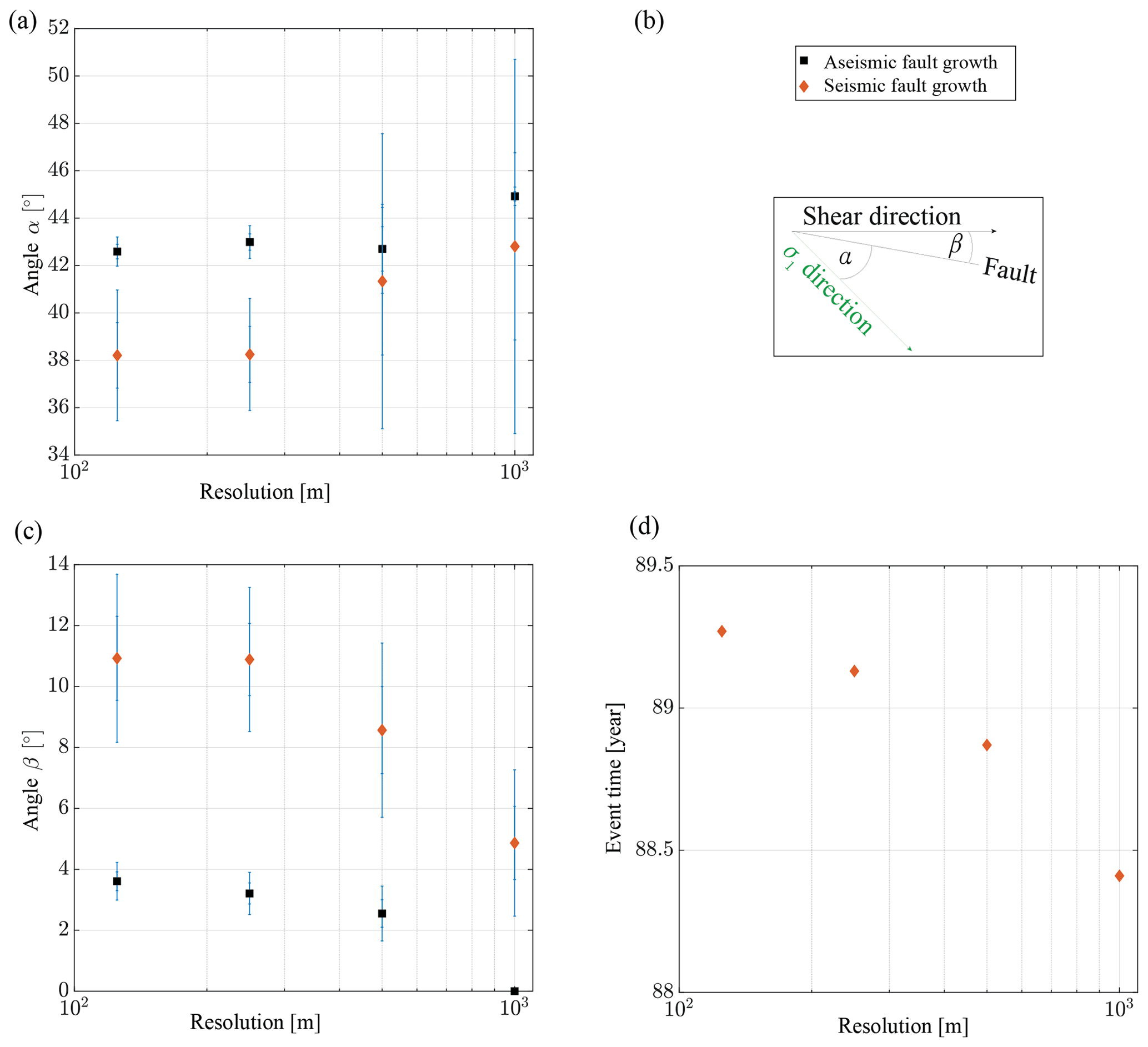
Figure A1Convergence analysis of fault angle and earthquake time as a relation between grid resolution and fault angles and between grid resolution and earthquake time start, respectively. The analysis shows that all seismic and aseismic fault angles as well as earthquake timing converge with grid size. Color-filled symbols indicate different faulting stages. Blue error bars correspond to errors in measuring the absolute angle β and to spatial variations of the σ1 direction at the fault tip (details are explained in Preuss et al., 2019). The solid line corresponds to the standard deviation [] and the dashed line to the standard deviation []. (a) Grid resolution in meter versus relative fault angle (see schematic illustration in c). (b) Grid resolution in meters versus absolute fault angle β. (c) Fault angle legend and schematic illustration of fault angles. (d) Grid resolution in meters versus the temporal onset of the earthquake in years.
The repository cited in the references (https://doi.org/10.3929/ethz-b-000397242; Preuss et al., 2020) contains five videos showing the temporal evolution of the four reference models and model HPT, which are all discussed in the main text.
SP designed the study, implemented and tested the 2.5-D approximation and the dynamically adaptive measure of fault width, designed the model setup, decided the parameter space, ran the simulations, gathered and interpreted the results, wrote the paper, and organized the submission process. JPA provided the initial idea to use the 2.5-D generalized Elsasser approach, helped clarify the results and improved the paper. TG provided the initial idea and tests of the dynamically adaptive measure of fault width, assisted in formulating the 2.5-D approximation for STM-RSF, and helped to design the initial model setup. YvD helped clarify the results and improved the paper.
The authors declare that they have no conflict of interest.
We thank Robert Herrendörfer for providing the STM-RSF code. We additionally thank André Niemeijer for a discussion on rate and state friction parameters for the bulk and Jianye Chen for giving very useful comments on the slip-velocity-dependent fault-width formulation. For constructive comments and discussions we thank the STM group at ETH Zurich. Numerical simulations were performed on the ETH clusters Leonhard and Euler. Perceptually uniform color maps are used in this study to prevent visual distortion of the data (Crameri, 2018). Lastly, we want to thank Michele Cooke for her constructive and well thought out commenting and Boris Kaus for clarifying an important detail about our implemented yield stress criteria.
This research has been supported by the Swiss National Science Foundation SNF (grant no. 200021_182069). Jean Paul Ampuero was supported by the French National Research Agency (ANR) through project FAULTS_R_GEMS (grant ANR-17-CE31-0008) and the Investments-in-the-Future project UCAJEDI (grant ANR-15-IDEX-01).
This paper was edited by David Healy and reviewed by Michele Cooke and Boris Kaus.
Alpar, B. and Yaltirak, C.: Characteristic features of the North Anatolian Fault in the eastern Marmara region and its tectonic evolution, Mar. Geol., 190, 329–350, https://doi.org/10.1016/S0025-3227(02)00353-5, 2002. a
Ampuero, J. P. and Mao, X.: Upper limit on damage zone thickness controlled by seismogenic depth, Fault Zone Dynamic Processes: Evolution of Fault Properties During Seismic Rupture, 227, 243, https://doi.org/10.1002/9781119156895.ch13, 2017. a, b, c, d, e, f, g, h, i, j, k, l
Ando, R., Shaw, B. E., and Scholz, C. H.: Quantifying natural fault geometry: Statistical of splay fault angles, B. Seismol. Soc. Am., 99, 389–395, https://doi.org/10.1785/0120080942, 2009. a
Andrews, D. J.: Rupture Propagation With Finite Stress in Antiplane Strain, J. Geophys. Res., 81, 3575–3582, https://doi.org/10.1029/JB081i020p03575, 1976. a
Andrews, D. J.: Rupture dynamics with energy loss outside the slip zone, J. Geophys. Res.-Sol. Ea., 110, 1–14, https://doi.org/10.1029/2004JB003191, 2005. a
Ashby, M. F. and Sammis, C. G.: The damage mechanics of brittle solids in compression, Pure Appl. Geophys., 133, 489–521, https://doi.org/10.1007/BF00878002, 1990. a
Aydin, A. and Berryman, J. G.: Analysis of the growth of strike-slip faults using effective medium theory, J. Struct. Geol., 32, 1629–1642, https://doi.org/10.1016/j.jsg.2009.11.007, 2010. a
Barka, A., Akyüz, H. S., Altunel, E., Sunal, G., Çakir, Z., Dikbas, A., Yerli, B., Armijo, R., Meyer, B., De Chabalier, J. B., Rockwell, T., Dolan, J. R., Hartleb, R., Dawson, T., Christofferson, S., Tucker, A., Fumal, T., Langridge, R., Stenner, H., Lettis, W., Bachhuber, J., and Page, W.: The surface rupture and slip distribution of the 17 August 1999 Izmit earthquake (M 7.4), North Anatolian fault, B. Seismol. Soc. Am., 92, 43–60, https://doi.org/10.1785/0120000841, 2002. a
Barth, N. C., Boulton, C., Carpenter, B. M., Batt, G. E., and Toy, V. G.: Slip localization on the southern Alpine Fault , New Zealand, Tectonics, 32, 620–640, https://doi.org/10.1002/tect.20041, 2013. a
Beeler, N. M., Tullis, T. E., Blanpied, M. L., and Weeks, J. D.: Frictional behavior of large displacement experimental faults, J. Geophys. Res.-Sol. Ea., 101, 8697–8715, https://doi.org/10.1029/96JB00411, 1996. a, b, c, d
Bhat, H. S., Dmowska, R., Rice, J. R., and Kame, N.: Dynamic slip transfer from the Denali to totschunda faults, Alaska: Testing theory for fault branching, B. Seismol. Soc. Am., 94, 202–213, https://doi.org/10.1785/0120040601, 2004. a
Bhat, H. S., Olives, M., Dmowska, R., and Rice, J. R.: Role of fault branches in earthquake rupture dynamics, J. Geophys. Res.-Sol. Ea., 112, 1–16, https://doi.org/10.1029/2007JB005027, 2007. a, b
Bhat, H. S., Rosakis, A. J., and Sammis, C. G.: A Micromechanics Based Constitutive Model for Brittle Failure at High Strain Rates, J. Appl. Mech., 79, 031016, https://doi.org/10.1115/1.4005897, 2012. a, b
Birren, T. and Reber, J. E.: The Impact of Rheology on the Transition From Stick-Slip to Creep in a Semibrittle Analog, J. Geophys. Res.-Sol. Ea., 124, 3144–3154, https://doi.org/10.1029/2018JB016914, 2019. a
Brace, W. F., Paulding, B. W., and Scholz, C.: Dilatancy in the fracture of crystalline rocks, J. Geophys. Res., 71, 3939–3953, https://doi.org/10.1029/jz071i016p03939, 1966. a
Brantut, N., Schubnel, A., Rouzaud, J., Brunet, F., and Shimamoto, T.: High-velocity frictional properties of a clay-bearing fault gouge and implications for earthquake mechanics, J. Geophys. Res., 113, 1–18, https://doi.org/10.1029/2007JB005551, 2008. a
Buiter, S. J. H., Babeyko, A. Y., Ellis, S., Gerya, T. V., Kaus, B. J., Kellner, A., Schreurs, G., and Yamada, Y.: The numerical sandbox: Comparison of model results for a shortening and an extension experiment, Geol. Soc. Spec. Publ., 253, 29–64, https://doi.org/10.1144/GSL.SP.2006.253.01.02, 2006. a
Cappa, F., Perrin, C., Manighetti, I., and Delor, E.: Off-fault long-term damage: A condition to account for generic, triangular earthquake slip profiles, Geochem., Geophy. Geosy., 15, 1476–1493, https://doi.org/10.1002/2013GC005182, 2014. a, b
Chen, J., Niemeijer, A. R., and Spiers, C. J.: Microphysically Derived Expressions for Rate-and-State Friction Parameters, a, b, and Dc, J. Geophys. Res.-Sol. Ea., 122, 9627–9657, https://doi.org/10.1002/2017JB014226, 2017. a
Chester, F. M. and Chester, J. S.: Ultracataclasite structure and friction processes of the Punchbowl fault, San Andreas system, California, Tectonophysics, 295, 199–221, https://doi.org/10.1016/S0040-1951(98)00121-8, 1998. a, b
Chester, F. M., Evans, J. P., and Biegel, R. L.: Internal structure and weakening mechanisms of the San Andreas Fault, J. Geodynam., 98, 771–786, https://doi.org/10.1029/92JB01866, 1993. a, b
Collettini, C., Carpenter, B. M., Viti, C., Cruciani, F., Mollo, S., and Tesei, T.: Fault structure and slip localization in carbonate-bearing normal faults: An example from the Northern Apennines of Italy, J. Struct. Geol., 67, 154–166, https://doi.org/10.1016/j.jsg.2014.07.017, 2014. a, b
Cooke, M.: Fracture localization along faults with spatially varying friction, J. Geophys. Res., 102, 22425–22434, 1997. a, b, c
Cooke, M. L. and Madden, E. H.: Is the Earth Lazy? A review of work minimization in fault evolution, J. Struct. Geol., 66, 334–346, https://doi.org/10.1016/j.jsg.2014.05.004, 2014. a
Cooke, M. L. and Murphy, S.: Assessing the work budget and efficiency of fault systems using mechanical models, J. Geophys. Res.-Sol. Ea., 109, 1–13, https://doi.org/10.1029/2004JB002968, 2004. a
Cowie, P. A. and Scholz, C. H.: Growth of faults by accumulation of seismic slip, J. Geophys. Res., 97, 11085, https://doi.org/10.1029/92JB00586, 1992. a
Crameri, F.: Geodynamic diagnostics, scientific visualisation and StagLab 3.0, Geosci. Model Dev., 11, 2541–2562, https://doi.org/10.5194/gmd-11-2541-2018, 2018. a
Dieterich, J. H.: Constitutive properties of faults with simulated gouge, Geophys. Monogr. Ser., 24, 103–120, https://doi.org/10.1029/GM024p0103, 1981. a
Dooley, T. P. and Schreurs, G.: Analogue modelling of intraplate strike-slip tectonics: A review and new experimental results, Tectonophysics, 574–575, 1–71, https://doi.org/10.1016/j.tecto.2012.05.030, 2012. a
Drucker, D. C. and Prager, W.: Soil mechanics and plastic analysis or limit design, Q. Appl. Math., 10, 157–165, https://doi.org/10.1090/qam/48291, 1952. a
Erdogan, F. and Sih, G. C.: On the Crack Extension in Plates Under Plane Loading and Transverse Shear, J. Basic Eng.-T. ASME, 85, 519, https://doi.org/10.1115/1.3656897, 1963. a
Erickson, B. A., Dunham, E. M., and Khosravifar, A.: A finite difference method for off-fault plasticity throughout the earthquake cycle, J. Mech. Phys. Sol., 109, 50–77, https://doi.org/10.1016/j.jmps.2017.08.002, 2017. a
Fang, Z. and Dunham, E. M.: Additional shear resistance from fault roughness and stress levels on geometrically complex faults, J. Geophys. Res.-Sol. Ea., 118, 3642–3654, https://doi.org/10.1002/jgrb.50262, 2013. a
Faulkner, D. R., Mitchell, T. M., Healy, D., and Heap, M. J.: Slip on “weak” faults by the rotation of regional stress in the fracture damage zone, Nature, 444, 922–925, https://doi.org/10.1038/nature05353, 2006. a
Faulkner, D. R., Mitchell, T. M., Jensen, E., and Cembrano, J.: Scaling of fault damage zones with displacement and the implications for fault growth processes, J. Geophys. Res.-Sol. Ea., 116, 1–11, https://doi.org/10.1029/2010JB007788, 2011. a
Gabriel, A. A., Ampuero, J. P., Dalguer, L. A., and Mai, P. M.: Source properties of dynamic rupture pulses with off-fault plasticity, J. Geophys. Res.-Sol. Ea., 118, 4117–4126, https://doi.org/10.1002/jgrb.50213, 2013. a, b
Gercek, H.: Poisson's ratio values for rocks, Int. J. Rock Mech. Min., 44, 1–13, https://doi.org/10.1016/j.ijrmms.2006.04.011, 2007. a
Gerya, T. V. and Yuen, D. A.: Characteristics-based marker-in-cell method with conservative finite-differences schemes for modeling geological flows with strongly variable transport properties, Phys. Earth Planet. In., 140, 293–318, https://doi.org/10.1016/j.pepi.2003.09.006, 2003. a
Gerya, T. V. and Yuen, D. A.: Robust characteristics method for modelling multiphase visco-elasto-plastic thermo-mechanical problems, Phys. Earth Planet. In., 163, 83–105, https://doi.org/10.1016/j.pepi.2007.04.015, 2007. a, b
Han, R., Hirose, T., and Shimamoto, T.: Strong velocity weakening and powder lubrication of simulated carbonate faults at seismic slip rates, J. Geophys. Res., 115, B03412, https://doi.org/10.1029/2008JB006136, 2010. a
Hatem, A. E., Cooke, M. L., and Toeneboehn, K.: Strain localization and evolving kinematic efficiency of initiating strike-slip faults within wet kaolin experiments, J. Struct. Geol., 101, 96–108, https://doi.org/10.1016/j.jsg.2017.06.011, 2017. a
Herrendörfer, R., Gerya, T. V., and van Dinther, Y.: An Invariant Rate- and State-Dependent Friction Formulation for Viscoeastoplastic Earthquake Cycle Simulations, J. Geophys. Res.-Sol. Ea., 123, 5018–5051, https://doi.org/10.1029/2017JB015225, 2018. a, b, c, d, e, f, g, h
Hobbs, B. E., Mühlhaus, H. B., and Ord, A.: Instability, softening and localization of deformation, Geol. Soc. Spec. Publ., 54, 143–165, https://doi.org/10.1144/GSL.SP.1990.054.01.15, 1990. a
Hubert-Ferrari, A., King, G., Manighetti, I., Armijo, R., Meyer, B., and Tapponnier, P.: Long-term elasticity in the continental lithosphere; modelling the Aden Ridge propagation and the Anatolian extrusion process, Geophys. J. Int., 153, 111–132, https://doi.org/10.1046/j.1365-246X.2003.01872.x, 2003. a, b
Ickrath, M., Bohnhoff, M., Dresen, G., Martínez-Garzón, P., Bulut, F., Kwiatek, G., and Germer, O.: Detailed analysis of spatiotemporal variations of the stress field orientation along the Izmit-Düzce rupture in NW Turkey from inversion of first-motion polarity data, Geophys. J. Int., 202, 2120–2132, https://doi.org/10.1093/gji/ggv273, 2015. a
Ikari, M. J.: Principal slip zones: Precursors but not recorders of earthquake slip, Geology, 43, 955–958, https://doi.org/10.1130/G37028.1, 2015. a, b
Jenkins, J. T.: Localization in granylar materials, Appl. Mech. Rev., 43, 194–195, https://doi.org/10.1115/1.3120803, 1990. a
Jolivet, R., Lasserre, C., Doin, M. P., Peltzer, G., Avouac, J. P., Sun, J., and Dailu, R.: Spatio-temporal evolution of aseismic slip along the Haiyuan fault, China: Implications for fault frictional properties, Earth Planet. Sc. Let., 377-378, 23–33, https://doi.org/10.1016/j.epsl.2013.07.020, 2013. a
Jolivet, R., Simons, M., Agram, P. S., Duputel, Z., and Shen, Z. K.: Aseismic slip and seismogenic coupling along the central San Andreas Fault, Geophys. Res. Lett., 42, 297–306, https://doi.org/10.1002/2014GL062222, 2015. a
Kame, N. and Yamashita, T.: Dynamic branching, arresting of rupture and the seismic wave radiation in self-chosen crack path modelling, Geophys. J. Int., 155, 1042–1050, https://doi.org/10.1111/j.1365-246X.2003.02113.x, 2003. a, b
Kame, N., Rice, J. R., and Dmowska, R.: Effects of prestress state and rupture velocity on dynamic fault branching, J. Geophys. Res.-Sol. Ea., 108, 1–21, https://doi.org/10.1029/2002JB002189, 2003. a, b
Katz, Y., Weinberger, R., and Aydin, A.: Geometry and kinematic evolution of Riedel shear structures, Capitol Reef National Park, Utah, J. Struct. Geol., 26, 491–501, https://doi.org/10.1016/j.jsg.2003.08.003, 2004. a
Kim, Y. S., Peacock, D. C. P., and Sanderson, D. J.: Fault damage zones, J. Struct. Geol., 26, 503–517, https://doi.org/10.1016/j.jsg.2003.08.002, 2004. a, b
King, G. C. and Sammis, C. G.: The mechanisms of finite brittle strain, Pure Appl. Geophys., 138, 611–640, https://doi.org/10.1007/BF00876341, 1992. a
Lapusta, N. and Barbot, S.: Models of earthquakes and aseismic slip based on laboratory-derived rate and state friction laws, vol. 661, Research Signpost, Kerala, India, 2012. a
Lapusta, N., Rice, J. R., Ben-Zion, Y., and Zheng, G.: Elastodynamic analysis for slow tectonic loading with spontaneous rupture episodes on faults with rate- and state-dependent friction, J. Geophys. Res., 105, 23765, https://doi.org/10.1029/2000JB900250, 2000. a
Lavier, L. L., Buck, W. R., and Poliakov, A. N. B.: Factors controlling normal fault offset in an ideal brittle layer, J. Geophys. Res., 105, 23431, https://doi.org/10.1029/2000JB900108, 2000. a
Lee, S., Reber, J. E., Hayman, N. W., and Wheeler, M. F.: Investigation of wing crack formation with a combined phase-field and experimental approach, Geophys. Res. Lett., 43, 7946–7952, https://doi.org/10.1002/2016GL069979, 2016. a
Lehner, F. K., Li, V. C., and Rice, J. R.: Stress Diffusion Along Rupturing Plate Boundaries, J. Geophys. Res., 86, 6155–6169, 1981. a, b, c, d
Le Pichon, X., Chamot-Rooke, N., Rangin, C., and Sengör, A. M. C.: The North Anatolian fault in the Sea of Marmara, J. Geophys. Res.-Sol. Ea., 108, 1–20, https://doi.org/10.1029/2002jb001862, 2003. a
Lindsey, E. O. and Fialko, Y.: Geodetic constraints on frictional properties and earthquake hazard in the Imperial Valley, Southern California, J. Geophys. Res.-Sol. Ea., 121, 1097–1113, https://doi.org/10.1002/2015JB012516, 2016. a
Logan., J., Friedman, M., Higgs, M., Dengo, C., and Shimamoto, T.: Experimental studies of Simulated gouge and their application to studies of natural fault zones, U.S. Geo. Survey, Menlo Park, CA., Analysis, 305–343, 1979. a
Logan, J. M. and Rauenzahn, A. K.: Frictional dependence of gouge mixtures of quartz and montmorillonite on velocity, composition and fabric, Tectonophysics, 144, 87–108, https://doi.org/10.1016/0040-1951(87)90010-2, 1987. a
Logan, J. M., Dengo, C. A., Higgs, N. G., and Wang, Z. Z.: Fabrics of Experimental Fault Zones: Their Development and Relationship to Mechanical Behavior, vol. 51, Elsevier, https://doi.org/10.1016/S0074-6142(08)62814-4, 1992. a
Manighetti, I., King, G., and Sammis, C. G.: The role of off-fault damage in the evolution of normal faults, Earth Planet. Sc. Lett., 217, 399–408, https://doi.org/10.1016/S0012-821X(03)00601-0, 2004. a
Marone, C. and Kilgore, B.: Scaling of the critical slip distance for seismic faulting with shear strain in fault zones, Nature, 362, 618–621, https://doi.org/10.1038/362618a0, 1993. a, b, c
Marone, C., Hobbs, B. E., and Ord, A.: Coulomb constitutive laws for friction: Contrasts in frictional behavior for distributed and localized shear, Pure Appl. Geophys., 139, 195–214, https://doi.org/10.1007/BF00876327, 1992. a
Meyer, S. E., Kaus, B., and Passchier, C.: Development of branching brittle and ductile shear zones: A numerical study, Geochem. Geophy. Geosy., 18, 2054–2075, https://doi.org/10.1002/2016GC006793, 2017. a
Mitchell, T. M. and Faulkner, D. R.: The nature and origin of off-fault damage surrounding strike-slip fault zones with a wide range of displacements: A field study from the Atacama fault system, northern Chile, J. Struct. Geol., 31, 802–816, https://doi.org/10.1016/j.jsg.2009.05.002, 2009. a, b, c
Moore, D. E. and Byerlee, J.: Geometry of Recently Active Breaks Along the San Andreas Fault , California, Tech. rep., United States Department of the Interior – Geological Survey, https://doi.org/10.3133/ofr89347, 1989. a, b
Moore, D. E. and Byerlee, J. D.: Comparative geometry of the San Andreas Fault, California, and laboratory fault zones, Geol. Soc. Am. Bull., 103, 762–774, https://doi.org/10.1130/0016-7606(1991)103<0762:CGOTSA>2.3.CO;2, 1991. a, b, c
Moore, D. E. and Byerlee, J.: Relationships between sliding behavior and internal geometry of laboratory fault zones and some creeping and locked strike-slip faults of California, Tectonophysics, 211, 305–316, https://doi.org/10.1016/0040-1951(92)90067-G, 1992. a
Moore, D. E., Summers, R., and Byerlee, J. D.: Sliding behavior and deformation textures of heated illite gouge, J. Struct. Geol., 11, 329–342, https://doi.org/10.1016/0191-8141(89)90072-2, 1989. a
Mutlu, O. and Pollard, D. D.: On the patterns of wing cracks along an outcrop scale flaw: A numerical modeling approach using complementarity, J. Geophys. Res.-Sol. Ea., 113, 1–20, https://doi.org/10.1029/2007JB005284, 2008. a, b
Norris, R. J. and Toy, V. G.: Continental transforms: A view from the Alpine Fault, J. Struct. Geol., 64, 3–31, https://doi.org/10.1016/j.jsg.2014.03.003, 2014. a, b
Nur, A., Ron, H., and Scottti, O.: Kinematics and Mechanics of Tectonic Block Rotations, Geophysical, 49, 31–46, 1989. a
Okubo, K., Bhat, H. S., Rougier, E., Marty, S., Schubnel, A., Lei, Z., Knight, E. E., and Klinger, Y.: Dynamics, radiation and overall energy budget of earthquake rupture with coseismic off-fault damage, J. Geophys. Res.-Sol. Ea., 124, 11771–11801, https://doi.org/10.1029/2019jb017304, 2019. a, b, c, d
Paola, N. D., Holdsworth, R. E., Viti, C., Collettini, C., and Bullock, R.: Can grain size sensitive flow lubricate faults during the initial stages of earthquake propagation?, Earth Planet. Sc. Lett., 431, 48–58, https://doi.org/10.1016/j.epsl.2015.09.002, 2015. a
Peacock, D. C. and Sanderson, D. J.: Effects of layering and anisotropy on fault geometry, J. Geol. Soc., 149, 793–802, https://doi.org/10.1144/gsjgs.149.5.0793, 1992. a
Perrin, C., Manighetti, I., Ampuero, J.-P., Cappa, F., and Gaudemer, Y.: Location of largest earthquake slip and fast rupture controlled by along-strike change in fault structural maturity due to fault growth, J. Geophys. Res.-Sol. Ea., 2, 1–16, https://doi.org/10.1002/2015JB012671, 2016a. a, b
Perrin, C., Manighetti, I., and Gaudemer, Y.: Off-fault tip splay networks: A genetic and generic property of faults indicative of their long-term propagation, Comptes Rendus – Geoscience, 348, 52–60, https://doi.org/10.1016/j.crte.2015.05.002, 2016b. a, b, c, d, e, f, g
Plesch, A., Nicholson, C., Shaw, J., Marshall, S., Su, M.-H., and Maechling, P.: The SCEC Community Fault Model (CFM), available at: https://www.scec.org/research/cfm (last access: 28 May 2020), 2017. a
Poliakov, A. N. B., Dmowska, R., and Rice, J. R.: Dynamic shear rupture interactions with fault bends and off-axis secondary faulting, J. Geophys. Res.-Sol. Ea., 107, ESE 6–1–ESE 6–18, https://doi.org/10.1029/2001JB000572, 2002. a, b
Pozzi, G., Paola, N. D., Nielsen, S. B., Holdsworth, R. E., and Bowen, L.: A new interpretation for the nature and significance of mirror-like surfaces in experimental carbonate-hosted seismic faults, Geology, 46, 583–586, 2018. a
Preuss, S., Herrendörfer, R., Gerya, T. V., Ampuero, J., and Dinther, Y.: Seismic and Aseismic Fault Growth Lead to Different Fault Orientations, J. Geophys. Res.-Sol. Ea., 124, 8867–8889, https://doi.org/10.1029/2019jb017324, 2019. a, b, c, d, e, f, g, h, i, j, k, l, m, n, o
Preuss, S., Ampuero, J. P., Gerya, T. V., and van Dinther, Y.: Model data sets and videos to “Characteristics of earthquake ruptures and dynamic off-fault deformation on propagating faults”, ETH Zurich Research Collection, https://doi.org/10.3929/ethz-b-000397242, 2020. a
Price, R. J. and Kelly, A.: Deformation of age-hardened aluminium alloy crystals II. Fracture, Acta Metall. Mater., 12, 979–992, https://doi.org/10.1016/0001-6160(64)90070-7, 1964. a
Rawling, G. C., Baud, P., and Wong, T.-F.: Dilatancy, brittle strength, and anisotropy of foliated rocks: Experimental deformation and micromechanical modeling, J. Geophys. Res.-Sol. Ea., 107, ETG 8–1–ETG 8–14, https://doi.org/10.1029/2001jb000472, 2002. a
Rice, J. R.: The mechanics of earthquake rupture, Physics of the Earth's Interior, Amsterdam, North-Holland, 78th Edn., 1980. a, b
Rice, J. R.: Heating, weakening and shear localization in earthquake rupture Subject Areas, Philos. T. Roy. Soc. A, 375, https://doi.org/10.1098/rsta.2016.0015, 2017. a
Rice, J. R., Sammis, C. G., and Parsons, R.: Off-fault secondary failure induced by a dynamic slip pulse, B. Seismol. Soc. Am., 95, 109–134, https://doi.org/10.1785/0120030166, 2005. a, b, c
Riedel, W.: Zur Mechanik geologischer Brucherscheinungen, Centralbl. Mineral. Geol. u. Pal., 1929B, 354–368, 1929. a
Ritter, M. C., Rosenau, M., and Oncken, O.: Growing Faults in the Lab: Insights Into the Scale Dependence of the Fault Zone Evolution Process, Tectonics, 37, 140–153, https://doi.org/10.1002/2017TC004787, 2018a. a
Ritter, M. C., Santimano, T., Rosenau, M., Leever, K., and Oncken, O.: Sandbox rheometry: Co-evolution of stress and strain in Riedel- and Critical Wedge- experiments, Tectonophysics, 722, 400–409, https://doi.org/10.1016/j.tecto.2017.11.018, 2018b. a
Rubin, A. M. and Ampuero, J. P.: Earthquake nucleation on (aging) rate and state faults, J. Geophys. Res.-Sol. Ea., 110, 1–24, https://doi.org/10.1029/2005JB003686, 2005. a
Savage, H. M. and Brodsky, E. E.: Collateral damage: Evolution with displacement of fracture distribution and secondary fault strands in fault damage zones, J. Geophys. Res.-Sol. Ea., 116, https://doi.org/10.1029/2010JB007665, 2011. a, b, c
Savage, H. M. and Cooke, M. L.: Unlocking the effects of friction on fault damage zones, J. Struct. Geol., 32, 1732–1741, https://doi.org/10.1016/j.jsg.2009.08.014, 2010. a
Scholz, C. H., Dawers, N. H., Yu, J.-Z., Anders, M. H., and Cowie, P. A.: Fault growth and fault scaling laws: Preliminary results, J. Geophys. Res.-Sol. Ea., 98, 21951–21961, https://doi.org/10.1029/93JB01008, 1993. a
Scholz, C. H., Ando, R., and Shaw, B. E.: The mechanics of first order splay faulting: The strike-slip case, J. Struct. Geol., 32, 118–126, https://doi.org/10.1016/j.jsg.2009.10.007, 2010. a
Scuderi, M. M., Niemeijer, A. R., Collettini, C., and Marone, C.: Frictional properties and slip stability of active faults within carbonate, evaporite sequences: The role of dolomite and anhydrite, Earth Planet. Sc. Lett., 369–370, 220–232, https://doi.org/10.1016/j.epsl.2013.03.024, 2013. a
Scuderi, M. M., Collettini, C., Viti, C., Tinti, E., and Marone, C.: Evolution of shear fabric in granular fault gouge from stable sliding to stick slip and implications for fault slip mode, Geology, 45, 731–734, https://doi.org/10.1130/G39033.1, 2017. a, b
Segall, P. and Rice, J. R.: Dilatancy, compaction, and slip instability of a fluid-infiltrated fault, Nature, 100, 155–171, https://doi.org/10.1029/95JB02403, 1995. a
Sengör, A., Tüysüz, O., Imren, C., Sakinç, M., Eyidogan, H., Görür, N., Le Pichon, X., and Rangin, C.: The North Anatolian Fault: A New Look, Annu. Rev. Earth Pl. Sc., 33, 37–112, https://doi.org/10.1146/annurev.earth.32.101802.120415, 2004. a
Shipton, Z. K., Evans, J. P., Abercrombie, R. E., and Brodsky, E. E.: The Missing Sinks: Slip Localization in Faults, Damage Zones, and the Seismic Energy Budget, in: Earthquakes: Radiated Energy and the Physics of Faulting, Volume 170, edited by Abercrombie, R., McGarr, A., Toro, G. D., and Kanamori, H., Geophysical Monograph Series 170, available at: http://sites.bu.edu/rea/files/2016/02/Shipton_etal2006_AGUmono.pdf (last access: 17 July 2020), 2006. a
Sibson, R. H.: Fault rocks and fault mechanisms, J. Geol. Soci., 133, 191–213, https://doi.org/10.1144/gsjgs.133.3.0191, 1977. a
Sibson, R. H.: Continental fault structure and the shallow earthquake source, J. Geol. Soc., 140, 741–767, https://doi.org/10.1144/gsjgs.140.5.0741, 1983. a, b
Sibson, R. H.: Thickness of the Seismic Slip Zone, B. Seismol. Soc. Am., 93, 1169–1178, https://doi.org/10.1785/0120020061, 2003. a
Sleep, N. H.: Ductile creep, compaction, and rate and state dependent friction within major fault zones, J. Geophys. Res.-Sol. Ea., 100, 13065–13080, https://doi.org/10.1029/94jb03340, 1995. a
Smith, S. A. F., Billi, A., Di Toro, G., and Spiess, R.: Principal Slip Zones in Limestone : Microstructural Characterization and Implications for the Seismic Cycle (Tre Monti Fault, Central Apennines, Italy), Pure Appl. Geophys., 168, 2365–2393, https://doi.org/10.1007/s00024-011-0267-5, 2011. a
Smith, S. A. F., Nielsen, S., and Toro, G. D.: Strain localization and the onset of dynamic weakening in calcite fault gouge, Earth Planet. Sc. Lett., 413, 25–36, https://doi.org/10.1016/j.epsl.2014.12.043, 2015. a
Swanson, M. T.: Fault structure, wear mechanisms and rupture processes in pseudotachylyte generation, Tectonophysics, 204, 223–242, https://doi.org/10.1016/0040-1951(92)90309-T, 1992. a, b
Swanson, M. T.: Late Paleozoic strike-slip faults and related vein arrays of Cape Elizabeth, Maine, J. Struct. Geol., 28, 456–473, https://doi.org/10.1016/j.jsg.2005.12.009, 2006. a
Tchalenko, J. S.: Similarities between Shear Zones of Different Magnitudes, Geol. Soc. Am. Bull., 81, 1625–1640, https://doi.org/10.1130/0016-7606(1970)81[1625:SBSZOD]2.0.CO;2, 1970. a, b, c, d
Templeton, E. L. and Rice, J. R.: Off-fault plasticity and earthquake rupture dynamics: 1. Dry materials or neglect of fluid pressure changes, J. Geophys. Res.-Sol. Ea., 113, 1–19, https://doi.org/10.1029/2007JB005529, 2008. a, b, c
Toro, G. D., Goldsby, D. L., and Tullis, T. E.: Friction falls towards zero in quartz rock as slip velocity approaches seismic rates, Nature, 427, 436–439, https://doi.org/10.1038/nature02249, 2004. a
van Dinther, Y., Gerya, T. V., Dalguer, L. A., Corbi, F., Funiciello, F., and Mai, P. M.: The seismic cycle at subduction thrusts: 2. Dynamic implications of geodynamic simulations validated with laboratory models, J. Geophys. Res.-Sol. Ea., 118, 1502–1525, https://doi.org/10.1029/2012JB009479, 2013a. a, b, c
van Dinther, Y., Gerya, T. V., Dalguer, L. A., Mai, P. M., Morra, G., and Giardini, D.: The seismic cycle at subduction thrusts: Insights from seismo-thermo-mechanical models, J. Geophys. Res.-Sol. Ea., 118, 6183–6202, https://doi.org/10.1002/2013JB010380, 2013b. a, b, c
van Dinther, Y., Mai, P. M., Dalguer, L. A., and Gerya, T. V.: Modeling the seismic cycle in subduction zones: The role and spatiotemporal occurrence of off-megathrust earthquakes, Geophys. Res. Lett., 41, 1194–1201, https://doi.org/10.1002/2013GL058886, 2014. a
Vermilye, J. M. and Scholz, C. H.: The process zone: A microstructural view of fault growth, J. Geophys. Res., 103, 12223–12237, https://doi.org/10.1029/98JB00957, 1998. a
Wdowinski, S., Smith-Konter, B., Bock, Y., and Sandwell, D.: Diffuse interseismic deformation across the Pacific-North America plate boundary, Geol. Soc. Am., 35, 311–314, https://doi.org/10.1130/G22938A.1, 2007. a
Weng, H. and Ampuero, J. P.: The Dynamics of Elongated Earthquake Ruptures, EarthArXiv, https://doi.org/10.31223/osf.io/9yq8n, 2019. a, b
Willemse, E. J. M. and Pollard, D. D.: On the orientation and patterns of wing cracks and solution surfaces at the tips of a sliding flaw or fault, J. Geophys. Res.-Sol. Ea., 103, 2427–2438, https://doi.org/10.1029/97JB01587, 1998. a, b, c
Wollherr, S., Gabriel, A. A., and Mai, P. M.: Landers 1992 “Reloaded”: Integrative Dynamic Earthquake Rupture Modeling, J. Geophys. Res.-Sol. Ea., 124, 6666–6702, https://doi.org/10.1029/2018JB016355, 2019. a
Woodcock, N. H., Dickson, J. A. D., and Tarasewicz, J. P. T.: Transient permeability and reseal hardening in fault zones: evidence from dilation breccia textures, Geol. Soc. Spec. Publ., 270, 43–53, https://doi.org/10.1144/gsl.sp.2007.270.01.03, 2007. a