Characterizing a decametre-scale granitic reservoir using ground-penetrating radar and seismic methods

Ground-penetrating radar (GPR) and seismic imaging have proven to be important tools for the characterization of rock volumes. Both methods provide information about the physical rock mass properties and geological structures away from boreholes or tunnel walls. Here, we present the results from a geophysical characterization campaign that was conducted as part of a decametre-scale hydraulic stimulation experiment in the crystalline rock volume of the Grimsel Test Site (central Switzerland). For this characterization experiment, we used tunnel-based GPR reflection imaging as well as seismic travel-time tomography to investigate the volumes between several tunnels and boreholes. The interpretation of the GPR data with respect to geological structures is based on the unmigrated and migrated images. For the tomographic analysis of the seismic first-arrival travel-time data, we inverted for an anisotropic velocity model described by the Thomsen parameters v₀, ϵ and δ to account for the rock mass foliation. Subsequently, the GPR and seismic images were interpreted in combination with the geological model of the test volume and the known in situ stress states. We found that the ductile shear zones are clearly imaged by GPR and show an increase in seismic anisotropy due to a stronger foliation, while they are not visible in the p-wave (v₀) velocity model. Regions of decreased seismic p-wave velocity, however, correlate with regions of high fracture density. For geophysical characterization of potential deep geothermal reservoirs, our results imply that wireline-compatible borehole GPR should be considered for shear zone characterization, and that seismic anisotropy and velocity information are desirable to acquire in order to gain information about ductile shear zones and fracture density, respectively.

1 Introduction

Crystalline rock has been identified as the key host rock for geothermal energy exploitations (Brown et al., 2012). The detailed geophysical and geological characterizations of crystalline rock volumes are important steps in planning and managing geothermal reservoirs (e.g. Schmelzbach et al., 2016). Before exploiting geothermal energy, the hydraulic transmissivity within the reservoir needs to be enhanced to allow for sufficient fluid flow at depths where temperatures are adequately high. Within crystalline rock, fractures are the most important fluid flow pathways. Thus, the goal is to enhance their transmissivities and connectivities by high-pressure fluid injections (so-called hydraulic stimulations). To this end, the key property to be characterized in crystalline rock is the geometrical characteristics, i.e. location, orientation, density as well as fracture length and aperture. However, quantification of fracture length and aperture is challenging. The local fracture densities may also lead to local heterogeneities in the in situ stress field (e.g. Bell et al., 1992; Valley and Evans, 2010) and consequently impact the rock mass response to hydraulic stimulations. Additionally, the rock mass anisotropy (i.e. of elasticity, strength, etc.) is of importance as it can influence the propagation direction of induced fractures (Gischig et al., 2018).

Available geological information originates mostly from the mapping of rock outcrops and tunnel walls, and from borehole data (e.g. geophysical and geological core and borehole logging). Direct sampling is thus restricted to accessible locations leading to highly fragmented data sets with limited spatial coverage. To improve the spatial coverage, inter- and extrapolation between these highly fragmented data are required. While such inter- and extrapolation can be reliably performed in settings with high borehole density (e.g. Krietsch et al., 2018a), it can lead to high uncertainties in situations with sparse control data and/or significant spatial heterogeneity (Wellmann et al., 2010, 2014; Wellmann and Caumon, 2018).

Geophysical imaging can help to infer geological structures in the rock mass away from boreholes and tunnels. In particular, ground-penetrating radar (GPR), as well as seismic imaging and tomography have been shown to work well for tracing geological structures in crystalline rock (Schmelzbach et al., 2007). The challenge of imaging structures within crystalline rock with geophysical methods is that the rock mass appears typically quite homogeneous on large scales with respect to its mechanical properties (i.e. no layering or geological sequencing is observable). Nevertheless, fractures and shear zones cause local perturbations of these mechanical properties and dominate the hydraulic flow field and particle transport. As fractures only change the rock properties very locally (e.g. due to hydraulic and mechanical fracture apertures in the submillimetre range), individual fractures may remain undetected by geophysical methods that have a spatial resolution in the metre range and hence only allow resolving bulk properties representative of a certain volume.

GPR is one of the highest-resolution geophysical imaging method that may allow recording the reflections from individual fractures in crystalline rock. Applications of GPR methods offer the potential to constrain both the geometry and hydraulic properties of fractured rock formations. Pioneering tests of GPR reflection and ray-based transmission methods for characterizing shear zones, fractures and intrusions in granitic rock date back to the 1980s (Falk et al., 1987; Olsson et al., 1987, 1988, 1992; Sandberg et al., 1989). Experiments conducted in underground laboratories at Äspö in Sweden and the Grimsel Test Site (GTS) in Switzerland demonstrated that shear zones and lamprophyre dykes could be clearly identified in GPR images (Falk et al., 1987). In salt tracer tests at GTS, the tracer flow through permeable fractures was visualized using GPR cross-hole amplitude tomography (Niva et al., 1988). More recently, Dorn et al. (2012) have shown how water-bearing fractures in a granitic rock could be imaged using multi-offset single-hole and cross-hole GPR techniques. As demonstrated in laboratory experiments (Grégoire and Hollender, 2004), even the fracture aperture can be estimated from GPR data if the fracture filling is known.

Besides GPR investigations, seismic methods offer excellent opportunities to characterize crystalline rock masses as found at GTS. In particular, transmission experiments, such as cross-hole tomography, can provide valuable information on the presence or absence of fracture zones (Maurer and Green, 1997; Vasco et al., 1996, 1998). Seismic investigations at GTS also provided clear evidence that the seismic anisotropy of the intact rock cannot be neglected (Vasco et al., 1998), which complicates the analysis of seismic data. Nevertheless, the anisotropy parameters determined in rock volumes of intact rock and rock mass can provide valuable diagnostics on fracture orientations (e.g. Boadu and Long, 1996). Numerical experiments by Rubino et al. (2017) show the first evidence that also the fracture connectivity can significantly reduce the anisotropy of a rock mass.

Theoretical considerations combined with experimental data show that seismic velocity is influenced by the fracture density (i.e. an increased fracture density leads to a decrease in seismic velocity), the length of fractures intersecting a ray path, the fraction of the fracture in contact and the fracture filling (Boadu and Long, 1996). There are, however, other factors altering seismic velocity, such as mineralogical rock composition, pore space and its filling, and the in situ stress field. The fidelity of seismic velocity as a proxy for fracture density is thus rock type and site specific.

The link between seismic velocity and in situ stresses is evident from laboratory studies (e.g. Holt et al., 1996). For field studies, seismic velocities have been used to estimate in situ stresses before drilling into hydrocarbon reservoirs (Sayers et al., 2002). However, it is not generally possible to infer in situ stresses from seismic velocities due to the abovementioned factors that influence velocity. In contrast, transient poro-elastic stress changes can be imaged using seismic time-lapse tomography, as all factors except effective stresses remain the same (Doetsch et al., 2018b; Rivet et al., 2016; Schopper et al., 2020). The study presented here was conducted within the framework of the In-situ Stimulation and Circulation (ISC) project (Amann et al., 2018; Doetsch et al., 2018a) in the crystalline rocks at GTS in central Switzerland. The ISC project addresses key scientific questions related to hydraulic stimulation aspects of enhanced geothermal systems (EGSs), including a detailed reservoir characterization before and after the stimulation treatments. The crystalline target rock mass was carefully characterized with respect to its geological, hydraulic, mechanical and geophysical properties. Here, we present the results of the pre-stimulation geophysical characterization and interpret them in the context of the geology (Krietsch et al., 2018a) and in situ stress field (Krietsch et al., 2019). Prior to the experiments, our results supported the planning and design of the stimulation experiments, and later helped improve the interpretation of the stimulation experiments.

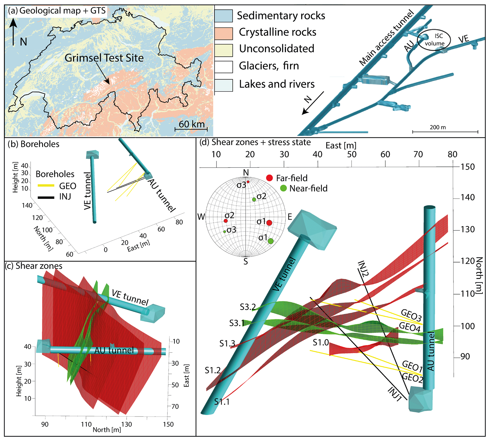
Figure 1 Location of GTS within Switzerland along with an overview of GTS (a) and ISC test volume with drilled boreholes (b). The geologically interpolated shear zones are visualized in panels (c) and (d). Panel (c) looks towards the west with an inclination of ∼30^∘. The orientations of the principal stress components for the perturbed (near-field) and unperturbed (far-field) stress fields are plotted in a lower hemisphere stereo net (d).

2 Site description

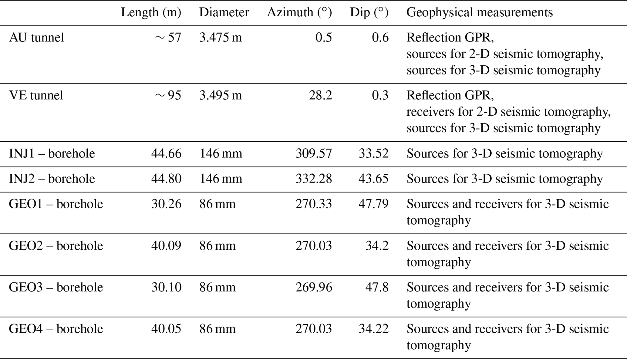
GTS is hosted within the crystalline rocks of the central Aar Massif in central Switzerland and operated by the Swiss National Cooperative for the Disposal of Radioactive Waste (Nagra). GTS is an underground research facility with an overburden of ∼480 m. The test volume of the ISC project has a size of approximately 20 m × 20 m × 20 m and is located at the very southern end of the laboratory and accessible from three tunnels (Fig. 1). For this study, measurements only along the tunnel walls of the AU and VE tunnels were conducted. Both tunnels were drilled with a tunnel-boring machine (TBM), resulting in an excavation damage zone of 0.4 to 1.5 m (Frieg et al., 2012) and smooth walls that easily allow measurements on the tunnel walls. In addition to the tunnels, two boreholes dedicated to high-pressure fluid injections (INJ holes) and four boreholes dedicated to geophysical monitoring (GEO holes) were used for geophysical borehole measurements (see Table 1).

Table 1 Overview of tunnels and boreholes used for geophysical measurements.

2.1 Geology

The ISC test volume is located at the lithological boundary between the central Aar granite (CAGr) and the Grimsel granodiorite (GrGr) (Keusen et al., 1989). These lithologies are close to the mineralogical transition between granitic and granodioritic rocks, and similar in quartz content (Wenning et al., 2018). The major mineralogical difference between CAGr and GrGr is their amount in sheet silicate minerals (biotite and white mica) (Wehrens et al., 2016). The rocks of these lithologies intruded the crystalline crust in the post-Variscan (Schaltegger and Corfu, 1992) and were subjected to Alpine deformation. During the latest phase of differentiation of the plutonic bodies, NW-striking, SE-dipping zones of weakness were initiated, along which aplitic dykes and lamprophyres intruded (Steck, 1968; Wehrens et al., 2016). The rock mass was metamorphosed with peak pressures of 6.5 kbar and temperatures around 450 ^∘C during the Alpine orogeny (Goncalves et al., 2012).

Simultaneously with the metamorphosis, the rock mass was deformed firstly in a ductile manner and later during exhumation in a brittle–ductile manner. Two shear zone orientations can be distinguished within the test volume. The older shear zone orientation (S1) strikes NE–SW with a dip towards SE formed in thrusting regime under ductile conditions (see Fig. 2 and Wehrens et al., 2016). Parallel to this S1 orientation, a pervasive foliation characterized by a preferential alignment of sheet silicates formed in the rock mass.

Figure 2 Overview geological structures and in situ stress field. The figure is reproduced from Krietsch et al. (2018a).

The younger shear zone orientation (S3) strikes E–W with a subvertical dip towards south. S3 shows a dextral strike-slip movement. Wherever the orientation of the metabasic dykes (i.e. metamorphosed lamprophyres) is aligned with the S3 direction, the shear zones localized within those dykes (Fig. 2). During the late phase of the S3-oriented shearing, brittle fractures formed, as well as milky quartz veins (Wehrens et al., 2016). These fractures often show a biotite coating, which indicates that this brittle deformation took place under green schist conditions when biotite is chemically stable. The uplift of the Aar Massif in the late Alpine stage induced some partly open tension joints (Steck, 1968; Wehrens et al., 2016). They seem to be the youngest features within the experimental test volume. Globally, the strike of the majority of the geological structures ranges between E–W and NE–SW (Fig. 2).

Krietsch et al. (2018a) identified four S1 and two S3 shear zones that crosscut the ISC test volume. Additionally, a highly fractured zone (up to 20 fractures per borehole metre) was identified in the eastern part of the test volume between the two S3 shear zones (Fig. 1).

2.2 In situ state of stress

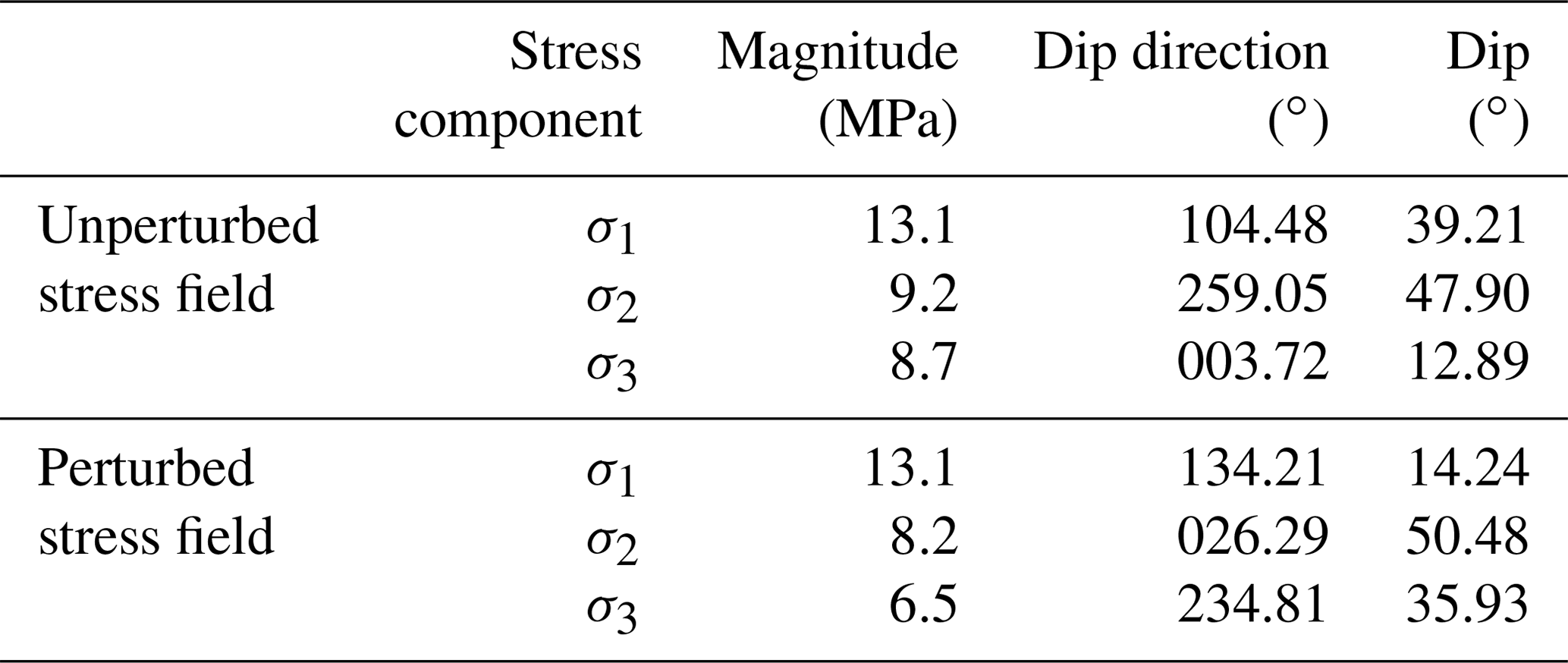
In addition to the geology, the in situ stress state within the test volume was characterized prior to the stimulation experiments (Krietsch et al., 2019). Based on the stress measurements, locations of two different principal stress measurement tensors were estimated for the description of the stress field. One tensor was measured far away (more than 30 m) from the shear zones (referred to as the unperturbed stress field), and the other tensor was derived from measurements at about 5 m from the shear zones (perturbed stress field). The unperturbed tensor has a maximum principal stress magnitude of 13 MPa which plunges 40^∘ towards the east (Table 2). The perturbed stress tensor indicates a maximum principal stress magnitude of 13 MPa that points subhorizontally towards the southeast (135^∘). The minimum principal stress component drops from 8.7 MPa far away from the shear zone to <3 MPa at the S3 shear zones. The detailed analysis of the in situ stress measurements has been described by Krietsch et al. (2019). Additional information on the in situ stress field and its heterogeneity was obtained during the 12 main hydraulic stimulation experiments of the ISC project (Dutler et al., 2019; Krietsch et al., 2020).

Table 2 Stress field information for the perturbed and unperturbed stress states (Krietsch et al., 2019). The perturbed stress tensor was measured at a distance of 5 m from the S3 shear zones.

3 Geophysical methods and data acquisition

With the aim of imaging geological structures within the rock volume of the ISC project, several geophysical characterization techniques were applied. GPR reflection imaging and seismic travel-time tomography were chosen due to the sensitivity of these methods to the location and orientation of shear zones, as well as to the mechanical rock properties, such as fracture density. Previous tests have shown that the acquisition of high-quality data is achievable in the environment of the Grimsel Test Site (e.g. Niva et al., 1988; Falk et al., 1987; Olsson et al., 1988; Vasco et al., 1998; Maurer and Green, 1997). Other techniques, such as electrical resistance tomography (ERT) or frequency-domain electromagnetic (EM) methods, were considered but not found suitable. For both methods, the electrical and metallic installations at GTS are a major obstacle, in particular the grounding cables through the tunnels, which channel the injected or induced electrical current, limiting the ability to investigate the highly resistive rock volume. In addition, for the ERT, the electrode–rock coupling is difficult, as the rock has a very high resistivity (>10 000 Ωm), which makes galvanic coupling and injection of a current very challenging. For GPR, the high resistivity of the rock is a major advantage, as it ensures minimum damping of the propagating signal.

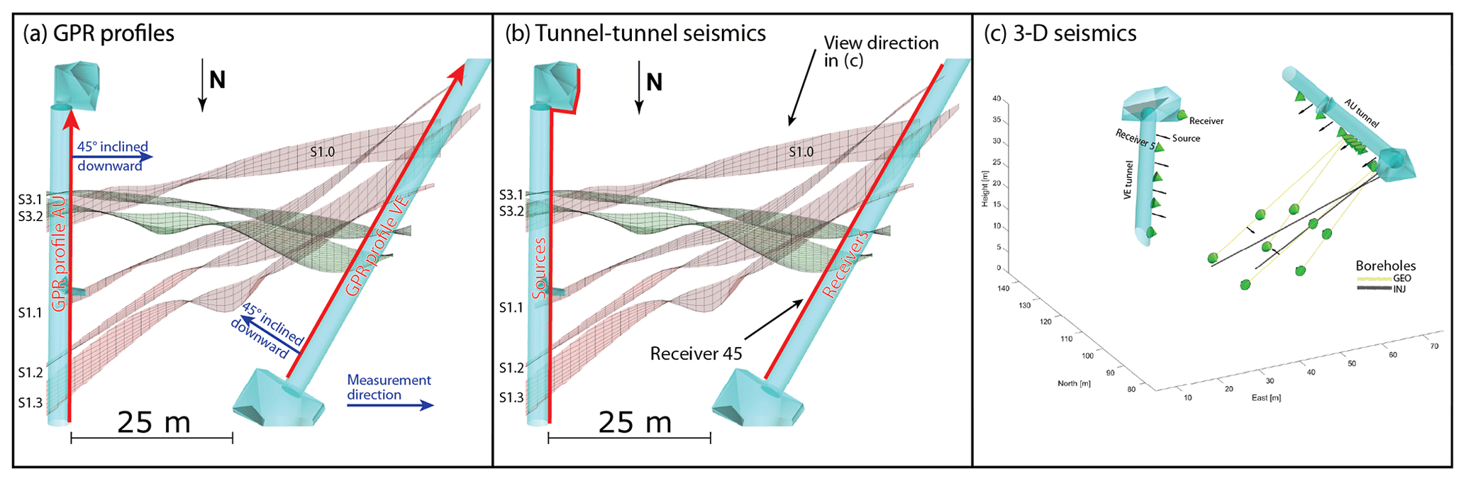
Figure 3 Acquisition geometry for the three geophysical data sets. GPR data were acquired using shielded antennas in the tunnels (a), the 2-D seismic data were acquired between the AU and VE tunnels (b), and the 3-D seismic data were acquired with both sources and receivers located in tunnels and boreholes (c).

3.1 Ground-penetrating radar (GPR)

The aim of the GPR imaging was to improve the geometrical information of the geological model for the ISC test volume. Structures of interest within the rock volume are the S1 and S3 shear zones, as well as individual fractures. In this study, we concentrated on the shear zones, as they cut through the entire test volume and were the target of hydraulic stimulations within the Grimsel ISC project. In order to improve the knowledge of the positions of the shear zones in the geological model, we jointly interpreted (i) unmigrated images and forward modelled data (Sect. 4.1) and (ii) the migrated and time-to-depth converted images (Sect. 4.2). This joint interpretation approach allowed constraining the location of the shear zones in 3-D even though the GPR data were acquired only along 2-D profiles. The interpretation of the 2-D migrated reflection images on its own may be affected by out-of-plane artefacts resulting from the geometry of subsurface features.

3.1.1 Data acquisition

GPR reflection data were acquired along the tunnel walls using shielded Malå high dynamic range (HDR) antennas with a nominal frequency of 160 MHz. The shielding of the antennas is important in this tunnel environment to ensure that strong interfering reflections from surface installations within the tunnels are attenuated. Other shielded antennas with frequencies between 80 and 250 MHz were tested as well, but the Malå HDR 160 MHz antennas were found to provide the best trade-off between resolution and depth penetration. Common-offset measurements with an antenna spacing of 0.33 m were performed in the VE and AU tunnels (Fig. 3a) with the imaging plane oriented in the direction of the experimental volume (approximately 45^∘ from the vertical towards the east and west, respectively). Traces were recorded every 5 cm along the two approximately 50 m long profiles. Data quality is high due to the low signal damping as a result of the high resistivity of the rock and due to relatively few reflectors in the target volume.

3.1.2 Processing of GPR data

Due to the very low electrical conductivity of the granitic rock, attenuation of the GPR signal was very low and data quality high. Processing of the constant-offset GPR data was performed using SeisSpace/Promax^® including the following steps (e.g. Schmelzbach et al., 2012):

1. setting up the geometry;

2. time zero correction;

3. top mute (mute arrivals before 25 ns);

4. amplitude gain using “time to power” of 2.25;

5. spectral whitening (whitening band: 140–300 MHz);

6. trace balancing (time window 40–500 ns);

7. automatic gain control (AGC; 300 ns window);

8. f–x deconvolution (in a sliding window);

9. Stolt migration using a constant velocity of 120 m µs⁻¹;

10. time-to-depth conversion (velocity of 120 m µs⁻¹).

The workflow and its parameters were fine tuned to enhance reflections in the GPR images. An initial data-independent amplitude scaling (in contrast to data-dependent scaling such as inverse envelope scaling) helped to increase signal amplitudes at later times, while not overly boosting remnants of surface reflections. The application of spectral whitening significantly suppresses mono-frequent ringing, whereas f–x deconvolution enhances coherent reflection events at the expense of random noise. A GPR velocity of 120 m µs⁻¹ was used for the migration and time-to-depth conversion. It was derived from cross-hole tomography and confirmed by testing different migration velocities by inspecting collapsing diffraction hyperbolae and the quality of other features.

For the interpretation, the migrated images are used to infer the position and characteristics of the shear zones. In addition, the unmigrated data (processed up to step 8) are compared with modelled GPR data using the 3-D geological model. The measurements on tunnel walls at unconventional (45^∘ side-looking) angles, as well as the orientation of the shear zones and other 3-D structures within the rock volume (tunnels, boreholes) render the interpretation of the acquired GPR data challenging. Therefore, to verify reflections from known structures and to potentially improve the geometrical information of these structures, we modelled the reflections of known structures based on the available 3-D geological model.

For each source–receiver combination and based on the existing 3-D geological model, a straight-ray-based modelling algorithm (Schmelzbach et al., 2007) was used to calculate the 3-D coordinates of the reflection points on each reflector. Then, assuming a constant velocity of 120 m µs⁻¹, the reflection travel times were computed and a Ricker wavelet was placed at the time of the reflection. Under the assumption of constant velocity and planar reflectors, this modelling provides arrival times of reflected waves that can be compared with the observed (unmigrated) reflection travel times to infer on the location and orientation of the planar reflectors. Displaying the modelled reflection times on top of the processed (up to step 8) but unmigrated data allowed us to identify and verify various reflections from key geological structures. Any observed mismatch between the modelled and measured reflection travel times can be used to improve the 3-D geological model.

3.2 Seismic methods

3.2.1 Tunnel–tunnel seismics

Seismic data were recorded between the AU and VE tunnels (Fig. 3b). A total number of 120 100 Hz resonance one-component geophones were installed at the VE tunnel walls at 0.5 m spacing, covering the western side of the experimental volume (Fig. 3b). Seismic signals were generated in the AU tunnel using a small hammer and a chisel. The 120 source points were separated by 0.5 m and covered the eastern side of the experiment.

The high quality of recorded seismic data allowed the picking of 9500 first-arrival travel times from the 14 400 total source–receiver combinations. The dominant frequency of the first-arriving seismic energy is ∼1.1 kHz. We estimated the picking uncertainty to be around 0.04 ms, corresponding to roughly 0.5 % of the travel times. Figure 4 shows a receiver gather for a geophone in the middle of the layout but north of the two S3 shear zones (location marked as “receiver 45” in Fig. 3b). The receiver gather shows a clear delay in the arrival times for all shots fired south of the two S3 shear zones (shot numbers 75–100). Another delay can be observed for the shot positions 40–42, which are located at the intersection of shear zone S3.2 and the AU tunnel. These arrival delays give the first hint for the influence of the shear zones on the seismic velocities.

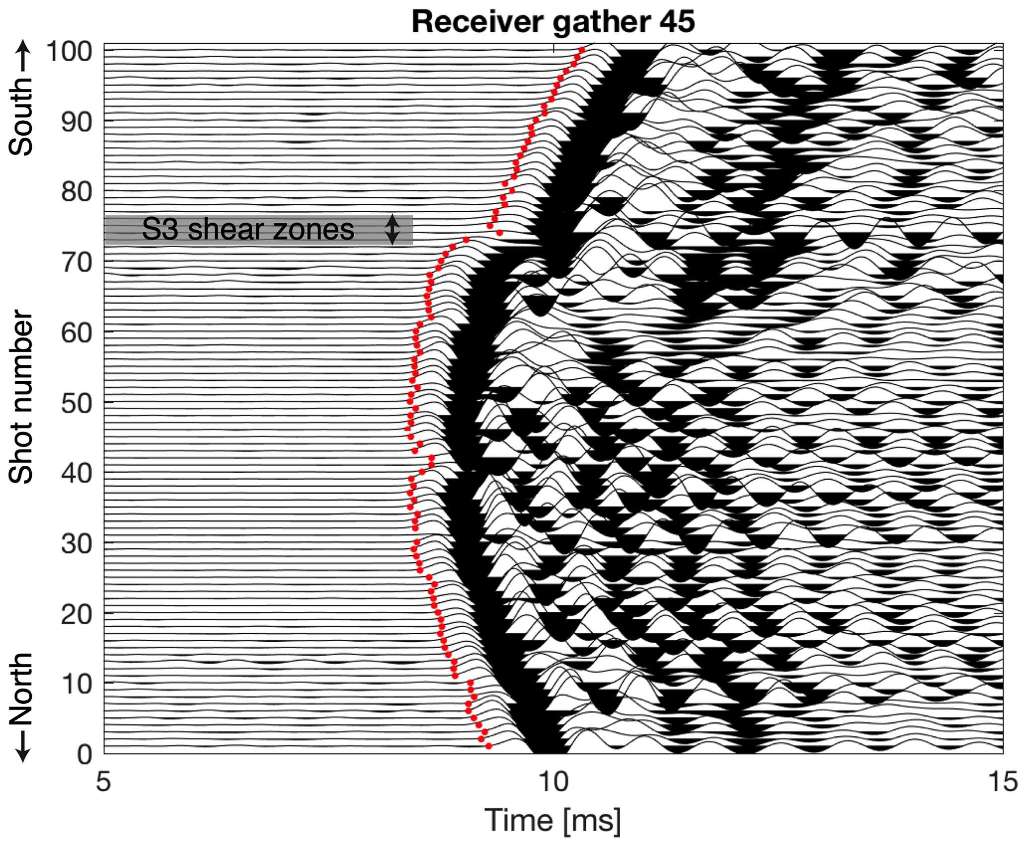
Figure 4 Seismic receiver gather for the tunnel–tunnel survey at a position north of the two S3 shear zones (location marked in Fig. 3b). A hammer source was used and data were recorded using 100 Hz geophones. The red dots mark the picked first arrivals. Delays in the arrivals can be observed for shot positions 40–42 and positions above 75.

3.2.2 Seismic characterization of the (3-D) volume

Seismic data for the 3-D tomography of the test volume were recorded using the 26 piezoelectric receivers installed for the passive seismic monitoring and sources in tunnels and boreholes (Fig. 3c, Doetsch et al., 2018a, b; Schopper et al., 2020). A sparker source was used in the six water-filled boreholes (INJ and GEO boreholes; see Table 1 and Fig. 1b), resulting in 448 source positions with a source spacing of 0.5 m along the boreholes. In addition, eight hammers placed in the AU and VE tunnels were used as sources. An example receiver gather (location marked as “receiver 5” in Fig. 3c) for all sparker sources in the INJ1 borehole is shown in Fig. 5. A total number of 10 050 first-arrival travel times were manually picked with an estimated uncertainty of 0.02 ms. In addition to the first arrivals that can be reliably picked, arrivals with a linear moveout in the receiver gather stand out in the data (Fig. 5). These events are recordings of secondary seismic waves that are generated by tube waves interacting with open fractures intersecting the source borehole. The sparker source generates a strong pressure pulse in the water-filled borehole. Some of the energy is transmitted through the rock, but another large part of the energy travels as a pressure wave within the water of the borehole. As this pressure wave interacts with open fractures intersecting the borehole, a part of the energy is transmitted into the surrounding rock. The fractures act as a source for secondary p waves (tube waves converted to p waves) that are recorded with a delay caused by the tube wave travelling from the sparker position along the borehole to the intersection of the borehole with the fracture. The secondary p waves have a linear moveout, because the distance between the scatter point and the receiver remains constant, and the tube-wave travel time is a linear function of the source depth in the borehole. The apparent velocity of the linear moveout is 1450 m s⁻¹, corresponding to the p-wave velocity in water. These linear-moveout features can be used to identify and characterize borehole-intersecting fractures, as the amplitude of these secondary waves depends on the fracture aperture and compliance (Hunziker et al., 2020).

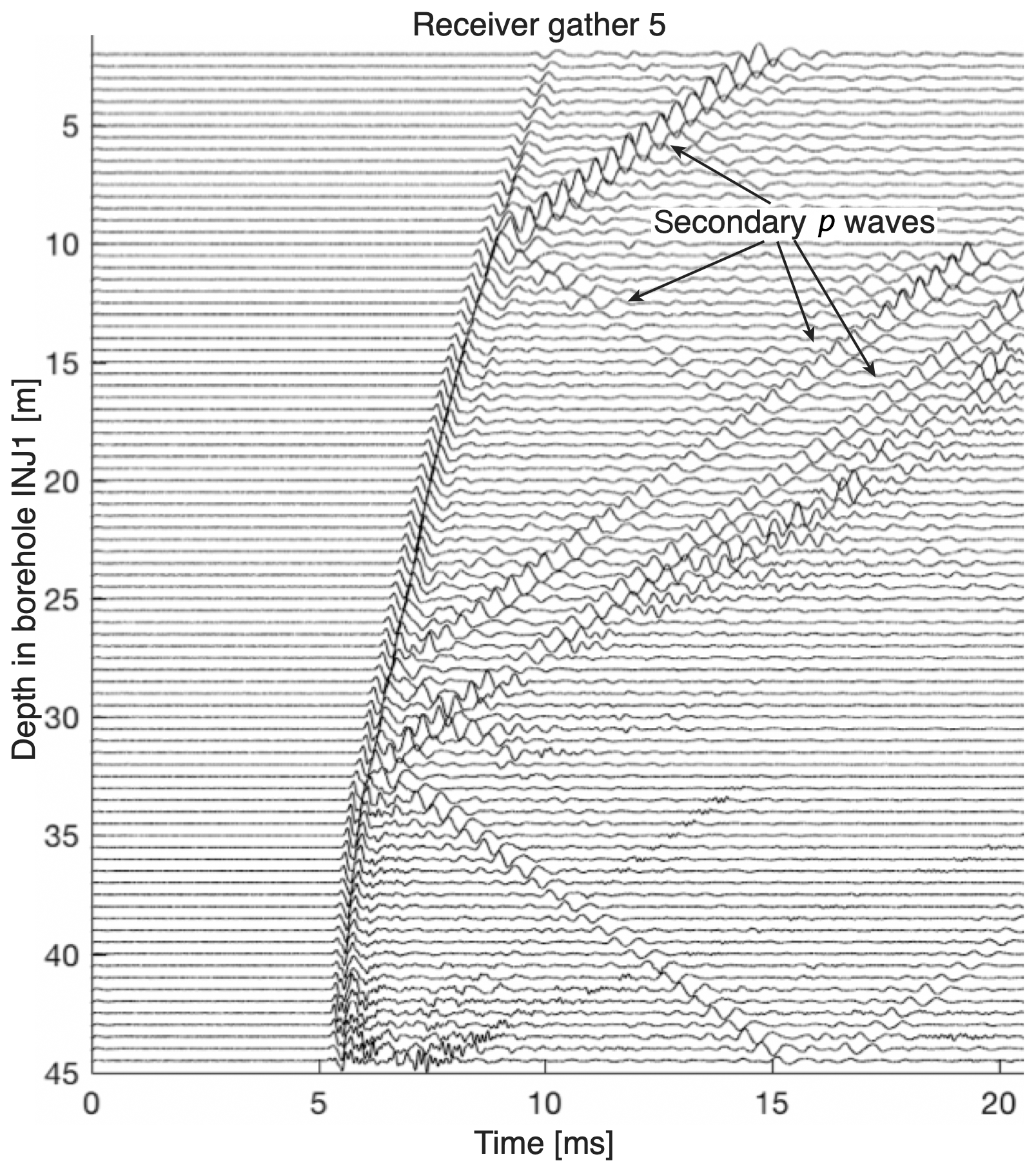
Figure 5 Example seismic data for one receiver and sources in one borehole. Data were recorded using a piezosensor at position 5 (marked in Fig. 3c), and a sparker source was used in borehole INJ1 at 0.5 m intervals. The linear features are secondary p waves, created by tube waves at the intersection with open fractures.

3.2.3 Anisotropic 2-D seismic travel-time tomography

Due to the foliation of the crystalline host rock within the test volume, the seismic velocity is anisotropic, which needs to be accounted for any travel-time tomography. For the 2-D anisotropic travel-time inversion, we extended the existing inversion framework presented by Doetsch et al. (2010) that uses the eikonal forward solver of Podvin and Lecomte (1991) and Tryggvason and Bergman (2006). We use the parameterization of Thomsen (1986) for weak seismic anisotropy in a transversely isotropic medium, with the velocity v_p at an angle θ to the symmetry axis normal of the anisotropy plane given by

$$\begin{array}{}\text{(1)}& v_{\mathrm{p}}\left(\mathit{\theta }\right)=v_{\mathrm{0}}\cdot \left(\mathrm{1}+\mathit{\delta }{\sin }^{\mathrm{2}}\mathit{\theta }{\cos }^{\mathrm{2}}\mathit{\theta }+\mathit{ϵ}{\sin }^{\mathrm{4}}\mathit{\theta }\right).\end{array}$$

v₀ is the velocity in the direction normal to the anisotropy plane, and ϵ and δ correspond to the strength of the anisotropy. ϵ represents the relative difference between the slow velocity v₀ and the fast velocity v_p(90^∘) within the anisotropy plane: $v_{\mathrm{p}}\left(\mathrm{90}{}^{\circ }\right)/v_{\mathrm{0}}=\mathrm{1}+\mathit{ϵ}$. The parameter δ is related to the ellipticity of the anisotropy.

The inversion framework was set up in a way that 2-D models of the parameters v₀, ϵ and δ were estimated simultaneously. It is also possible to simultaneously invert for the direction of the anisotropic symmetry axis, if this axis lies within the 2-D inversion plane. If the anisotropic symmetry axis points out of the inversion plane, it is not possible to invert for the direction of this symmetry axis, because 2-D data are not sufficient to constrain the two anisotropy angles. Therefore, in the case of a 2-D inversion, the direction of the symmetry axis has to be prescribed, and it is not possible to invert for it. For the Grimsel Test Site, we know the direction of the seismic anisotropy from the direction of foliation, determined in the geological characterization. This direction, which is oblique to the inversion plane, was thus prescribed in the inversion.

For the calculation of the ray paths, we assume that the ray paths are not affected by anisotropy. This assumption is only valid for cross-hole or cross-tunnel geometries and if the anisotropy is weak, which is given for our experiments. The travel times are calculated from the ray paths by calculating the travel time in each model cell using Eq. (1) and summing these times up along each ray path. The sensitivity or Jacobian matrix for the anisotropy parameters are also calculated using Eq. (1), as well as the ray path information (see the Supplement for details).

In addition to the estimation of the velocity and anisotropy parameters, the inversion algorithm also allows inverting for source and receiver static time shifts. These time shifts for individual sources and receivers can compensate local effects around the source and receiver positions, thereby improving the quality and consistency of the velocity and anisotropy parameter fields.

3.2.4 3-D seismic travel-time tomography

For the anisotropic travel-time tomography of the seismic 3-D data set, we perform a two-step inversion. First, we invert for global values of v₀, ϵ and δ, while prescribing the anisotropic symmetry axis. In a second step, we fix the values of ϵ and δ to the result of the first inversion in order to estimate the 3-D heterogeneity of v₀. We thus assume the direction of the anisotropic symmetry axis to be known and the Thomsen parameters ϵ and δ (Eq. 1) to be constant throughout the test volume. These assumptions are necessary, as the 3-D ray coverage in our experiment is not sufficient to invert for 3-D distributions of v₀, ϵ and δ as well as the two angles defining the symmetry axis. As for the 2-D tomography, the symmetry axis was assumed to be parallel to foliation. In the first step of the inversion, ϵ and δ are estimated by calculating the velocity for each source–receiver pair by dividing the source–receiver distance by the travel time and plotting these apparent velocities as a function of the angle between the ray path and the anisotropic symmetry axis. The assumed direction of the symmetry axis can thereby be verified by analysing the apparent velocity as a function of the angle to the symmetry axis. ϵ and δ are then estimated from fitting the anisotropic velocity of Eq. (1) to the angular velocity distribution. We found that this inversion problem is well constrained as it is highly overdetermined, with three parameters (ϵ, δ and v₀) and a large number of travel-time observations (>10 000 in this study).

In the second inversion step, the values of ϵ and δ, as well as the direction of the symmetry axis are then kept constant and only the heterogeneity in v₀ is estimated. This simplification allows for algorithms built for isotropic 3-D travel-time inversion to be used with minimal adjustment. Here, we use the inversion algorithm of Doetsch et al. (2010) that uses the eikonal solver of Podvin and Lecomte (1991) and Tryggvason and Bergman (2006).

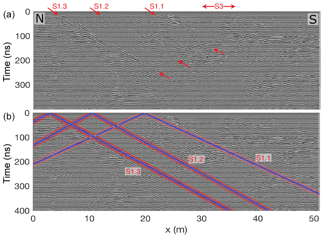
Figure 6 GPR reflection data measured from the AU tunnel in the N–S plane, looking west. These data are processed up to step 8 (Sect. 3.1.2) but not migrated. The shear zone locations inferred from the geological mapping are marked in panel (a). Panel (b) shows as an overlay GPR reflections, which were modelled based on known shear zone locations and their average orientation.

4 Results and interpretation

4.1 Comparison of unmigrated and modelled GPR data

Figure 6 shows the pre-processed (up to step 8) but unmigrated data acquired in the AU tunnel in the N–S plane, looking west. The three S1 shear zones are clearly visible in the radargram (arrows in Fig. 6a) and match the modelled reflections (Fig. 6b) very well. The geological model was already of high quality and only needed minor updates of the shear zone details to match the GPR data. Reflections from the two S3 shear zones are visible neither in the recorded nor in the modelled data, because these shear zones are perpendicular to the tunnel and thus do not create reflections for the side-looking GPR. The migrated data are shown in Fig. S1 in the Supplement.

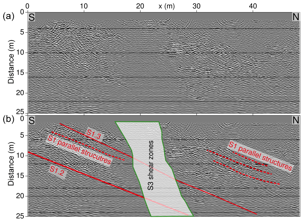
Figure 7 Fully processed and migrated GPR data acquired from the VE tunnel, along with its geological interpretation. Panels (a) and (b) show the same GPR image. Additionally, in panel (b), the intersections with the geological structures inferred from the geological model are shown. Here, especially the complex intersection zone of the S1 and S3 shear zones is of interest.

4.2 Migrated GPR data

The fully processed data acquired in the VE tunnel were used to analyse the more complex shear zone geometry in this area, with the S1 shear zones being intersected by the two S3 shear zones. Figure S2 shows the unmigrated data and Fig. 7 shows the migrated and time-to-depth converted GPR data along with our interpretation. The S3 shear zones that intersect the volume and cut through the S1 shear zones are evident as areas of low reflectivity. The S3 shear zones intersect the VE tunnel at steep angles, which makes them poor reflectors in constant-offset GPR images recorded from the tunnel (compare with Fig. 6). Even the strongly fractured rock between the two S3 shear zones shows surprisingly little reflectivity, most likely due to fractures being parallel to the S3 shear zones. It is possible that they could have been imaged when rotating the antennas by 90^∘, but this was not tested in the field. Another reason for the little reflectivity might be the enrichment in phyllosilicates within the S3 shear zones, leading to an enhanced electrical conductivity (Wenning et al., 2018). In contrast, borehole GPR data recorded from the GEO boreholes (Fig. 1 and Table 1) clearly image the S3 shear zones and even monitoring of saline tracer migration between them is possible using borehole GPR (Giertzuch et al., 2020).

The S1 shear zones can be identified on both sides of the S3 shear zone in Fig. 7 but cannot be traced through them. Also, S1-parallel brittle structures can be identified on both sides of the S3 shear zones. These types of S1-parallel structures of limited length (here 5–10 m) occur throughout the experiment volume and are also evident in borehole logs. These features are likely associated with brittle deformation along the foliation planes. During the time of retrograde brittle deformation of the S1 shear zones, the S1-parallel foliation also might have been locally deformed under brittle conditions.

The shear zone geometry as imaged by GPR fits with the previous geological model and adds detail in form of the S1-parallel features, which were not previously mapped. GPR also adds detail information in the area of the intersecting shear zones, which is not accessed by boreholes.

4.3 Anisotropic 2-D seismic velocity model

The 9500 travel times (Sect. 3.2.1) were inverted for 2-D distributions of the Thomsen parameters v₀,ϵ and δ (Sect. 3.2.3), while fixing the direction of the anisotropy axis to the direction of the foliation of the rock. Figure 8 shows the result of the inversion, with a root mean square (rms) misfit of 0.04 ms (0.3 %–0.6 % of the travel times of 8–16 ms). In addition to the three parameter fields, source statics (standard deviation of 0.07 ms) were estimated to account for differences in the rock properties in the immediate vicinity of the source locations (Fig. 8d). Source statics are largest for sources within the shear zones (source numbers 40–42 and 70–75), where delays could already be observed in the raw waveforms (Fig. 4), as well as in the AU cavern. In contrast to the tunnels, which were TBM drilled, the AU cavern was blasted, which leads to a larger excavation damage zone and thus larger source statics.

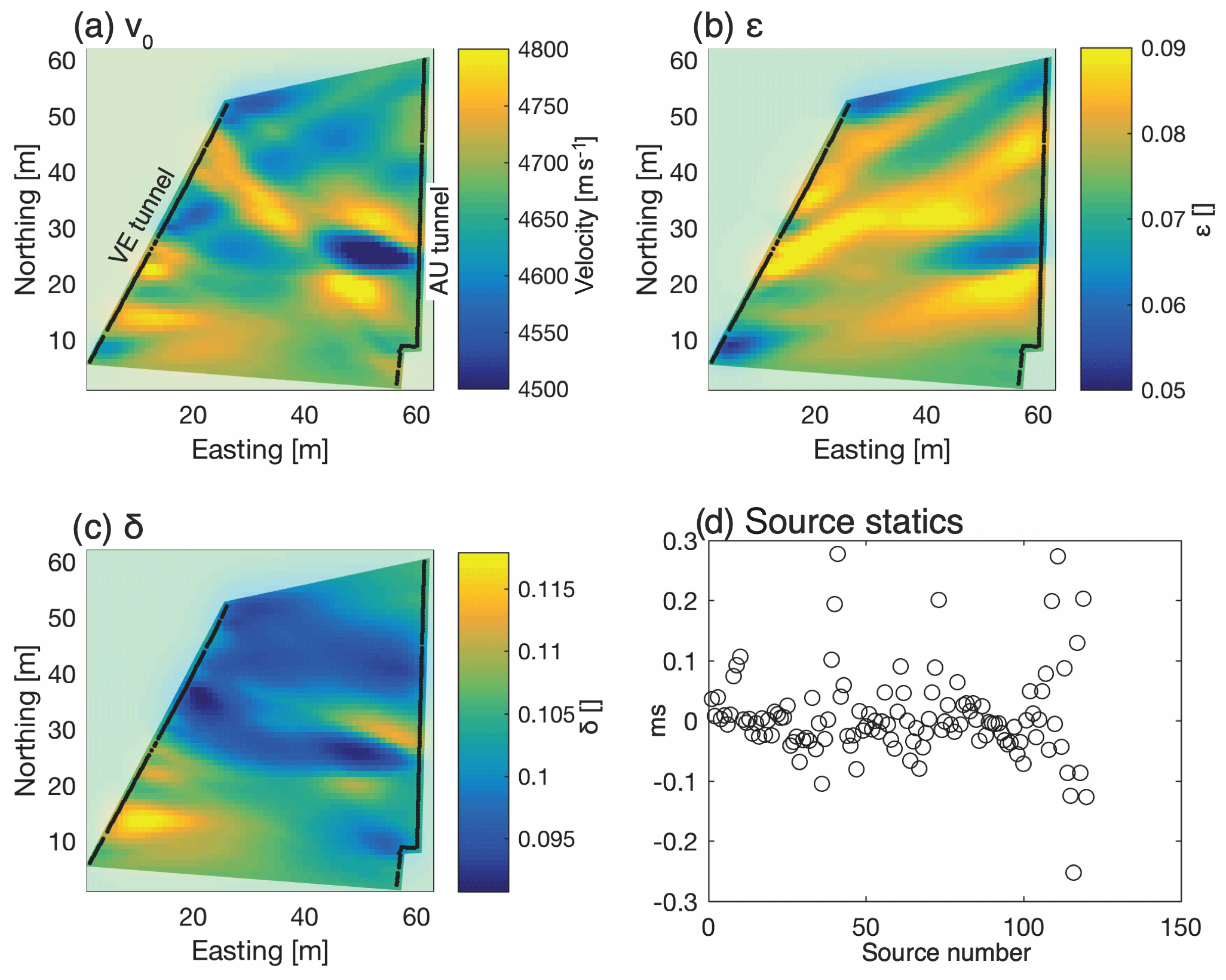
Figure 8 Results of the anisotropic 2-D tunnel–tunnel seismic travel-time tomography. The inversion estimates the three Thomsen (1986) parameters v₀ (a), ϵ (b) and δ (c) along with source statics (d) to account for rock quality differences around the source positions. Sources and receivers are marked as black dots.

The p-wave velocity in the direction of the anisotropic symmetry axis (v₀) in Fig. 8a shows a low-velocity zone in the east–west direction, adjacent to the AU tunnel as the main feature. Otherwise, the velocity is relatively homogeneous (±2 %). The dominant low-velocity zone is located between the positions of the two S3 shear zones and extends about 15–20 m west from the AU tunnel. The NE- to SW-striking S1 shear zones are not visible in the v₀ image. The ϵ model (Fig. 8b) shows the relative increase of velocity within the anisotropy plane, compared to the velocity in direction of the symmetry axis (v₀). The ϵ model shows several high-anisotropy features in northeast to southwest directions. These features coincide in direction and location with the S1 shear zones. In addition to the previously known shear zone strands that connect the AU and VE tunnels, a high-ϵ feature can be observed just south of the location of the S3 shear zones near the AU tunnel. While undetected during the geological characterization (Krietsch et al., 2018a), this feature has recently been verified as a fourth S1 shear zone.

Geologically, the S1 shear zones are characterized by an increase in foliation compared to the surrounding rock. As foliation is also the reason for the seismic anisotropy of the rock, it is no surprise that the increased foliation within the shear zones are detected as an increase of anisotropy. The model of δ (Fig. 8c), which characterizes the ellipticity of the anisotropy, shows only a minor variation and does not contribute to our interpretation of the results.

4.4 3-D velocity model

For the 3-D seismic travel-time data set, we first estimate the anisotropy parameters that are then assumed to be constant throughout the volume. The red dots in Fig. 9 show apparent velocity (source–receiver distance divided by travel time) as a function of angle from the symmetry axis. This velocity distribution confirms that the direction of the anisotropy axis is parallel to foliation, because the maximum velocity is at a 90^∘ angle to the symmetry axis (i.e. within the anisotropy plane) and the distribution is symmetric about the 90^∘ direction. A different symmetry axis would result in a shifted or skewed distribution. Fitting the anisotropy model of Eq. (1) to the apparent velocity distribution results in estimated values of ϵ=0.065 and δ=0.038, and the velocity distribution is shown as a green line in Fig. 9. The ϵ value is consistent with the 2-D result (Fig. 8b), while δ is slightly lower than the 2-D result (Fig. 8c). δ is not very well resolved and thus not interpreted. The scatter of the apparent velocity values around the estimated distribution shows the inhomogeneity of the rock, which we explain in our inversion by variations in v₀. Keeping the ϵ and δ values fixed, we use the 10 050 travel times to invert for the 3-D distribution v₀. We use a model with 2 m × 2 m × 2 m grid size and fit the data to the estimated error level of 0.02 ms.

Figure 9 Apparent velocities (source–receiver distance divided by travel time) plotted in red against the angle from the anisotropic symmetry axis. The green dots/line show the prediction of the fitted anisotropic velocity model (Eq. 1). The difference between the red and green dots is evidence for the heterogeneity of the rock and used in the 3-D inversion for v₀.

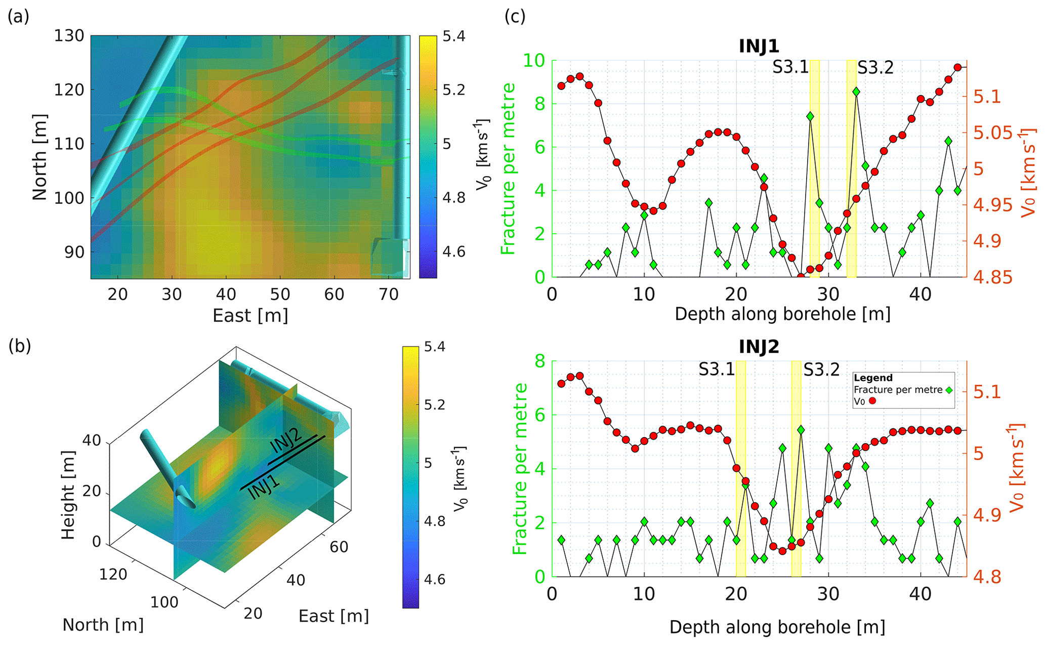
Figure 10 Results of the 3-D velocity inversion. Panels (a) and (b) show slices through the 3-D v₀ volume, along with the interpolated shear zones and the boreholes shown in panel (c). The horizontal cut in panel (a) is extracted 1 m below tunnel level. Panel (c) shows the velocity extracted from the 3-D volume along the trajectories of two boreholes along with the fracture count per metre. One can observe a decrease of velocity near the S3 shear zones and where fracture density is high.

Figure 10a and b show cut sections through the 3-D v₀ model. Similar to the 2-D image, the low-velocity zone between the S3 shear zones near the AU tunnel is the strongest feature. Horizontally, at the level of the tunnels, the low-velocity zone extends from the AU tunnel 15 m to the west, in agreement with the 2-D results. Vertically, the low-velocity zone extends downwards near the AU tunnel and extends further to the west at a depth of 20 m below the tunnels (15 m elevation). While extending vertically and in E–W direction, the N–S extent of the low-velocity zone is restricted to a few metres – approximately the extent between the two S3 shear zones. Similar to the 2-D velocity model, there is no evidence of the S1 shear zones in the tomogram.

5 Integration of geomechanical a priori knowledge and implications for hydraulic stimulations

The major aim of the GPR surveys was to constrain the knowledge on shear zone orientations and persistency for further spatial extrapolation away from tunnel and borehole intersections. The S1 shear zones could be traced in the unmigrated GPR image from the AU tunnel, as well as in the migrated image from the VE tunnel (see Sect. 4.1 and 4.2). Additional S1-parallel fractures have been identified inside the rock mass, which could not have been mapped during the geological characterization. This is in agreement with the observations from Krietsch et al. (2020) and Villiger et al. (2020). Both describe that fluid diffuses mostly along a single planar feature during the hydraulic stimulation experiments targeting S1 structures. In contrast to this, the S3 shear zones are poorly visible in the GPR images. Above, we named an increased fracture density between the S3 shear zones as potential explanation for the low reflectivity. This would fit again the interpretations from Krietsch et al. (2020) and Villiger et al. (2020), who argued that fluid diffuses within a complex fracture network when injected into S3 shear zones. Thus, the GPR survey helped to refine the geological model published by Krietsch et al. (2018a).

From 2-D seismic tomography, S1 and S3 could have been traced throughout the rock volume. The S1 shear zones are evident as an increase in anisotropy, visualized in the spatial variation of the Thomson parameter ϵ. We argue that this is caused by the more distinct foliation within these shear zones, compared to the overall host rock. Due to this more distinct foliation, the rock anisotropy (i.e. the contrast in stiffness normal and parallel to the foliation) becomes larger. In contrast, the dense fracturing within the S3 shear zones reduces elasticity anisotropy and thus is not visible in the ϵ variations. Nevertheless, it is clearly visible in the v₀ tomogram as zones of reduced velocity. This velocity reduction can have multiple reasons, for example, changes in elastic properties of the rock mass and/or variation within the in situ stress field. Wenning et al. (2018) described an enrichment in phyllosilicates as S3 shear zones are intersected. This, in combination with the enhanced fracture density between the S3 shear zones, may have resulted in locally reduced rock mass stiffness, strength and increased rock porosity, leading to a seismic velocity reduction. Interestingly, the zone of highest fracture density collocates with the lowest ϵ magnitudes. This is in agreement with Rubino et al. (2017), who described that with increasing fracture connectivity the velocity anisotropy reduces.

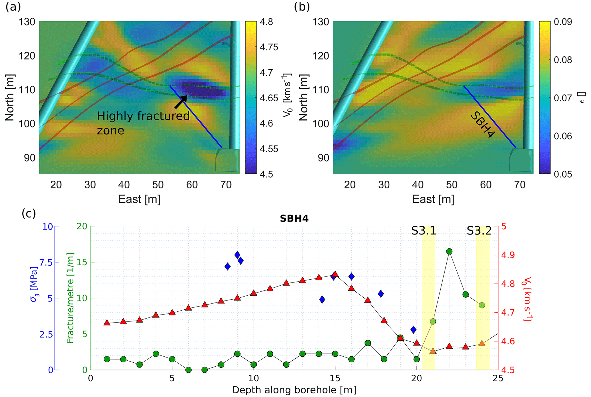
Figure 11 P-wave velocities (v₀) (a) and Thomsen's ϵ (b) from 2-D anisotropic inversion of the tunnel–tunnel seismic travel-time data, along with the three S1 shear zones and the SBH4 borehole. Panel (c) shows fractures per metre, the minimum in situ σ₃ stress and p-wave velocities (v₀) along borehole SBH4. Fracture density and σ₃ were measured within the borehole; velocity is extracted from panel (a).

To describe the influence of the rock mass elasticity, we compare the rheology and fracture density with the v₀ measurements (Fig. 11). We extract the velocities along the boreholes from the 2-D (borehole SBH4) and 3-D (boreholes INJ1 and INJ2) tomograms and use the velocity v₀ in the direction of the anisotropy axis, which coincides with the direction of foliation. Fractures were mapped along the boreholes using a combination of optical borehole televiewer images and core logs (Krietsch et al., 2018a). The fracture density values mapped along boreholes are biased by the borehole orientation with respect to fracture orientations, since, e.g. borehole-parallel fractures are very likely to be missed in the mapping. To overcome this influence, we transfer the longitudinal borehole observations (the so-called P₁₀) into volumetric estimates (the so-called P₃₂) (Dershowitz and Herda, 1992). Here, we follow the approach used by Brixel et al. (2020) for the same data set. Fracture frequency is generally low, mostly with three or fewer fractures per metre but increases towards the shear zones.

Along borehole SBH4, fracture density strongly increases as the S3 shear zones are penetrated. At a distance of 5 m from the shear zones along SBH4, v₀ starts to decrease, reaching its minimum between the two shear zones. It is expected that seismic velocity decreases with increasing fracture density (e.g. Boadu and Long, 1996). While our observations fit this expectation, also other factors influence seismic velocity. Thus, we cannot purely attribute the drop in v₀ to the increase in fracture density. For example, the S3 shear zones that bind the zone of high fracture density consists of metabasic dykes, which include an increase in phyllosilicates, highly sheared material and fault gouge. As mentioned earlier, the contrast in material compliance between host rock and metabasic dyke could have also led to a reduction in v₀. Generally, seismic velocities in the tomograms vary smoothly, which is primarily due to resolution limitations of the method as well as parameterization and regularization of the inversion. In contrast, measurements of fracture density depend on the aggregation interval and offset, but any two measurements are fully independent. Figures 10c and 11c show that all zones with low velocity are characterized by increased fracture density. The main geological features for low seismic velocities are the S3 shear zones, which are characterized by a high fracture density in all boreholes. Additionally, the interval of 8–12 m in borehole INJ1 shows intermediate to low velocities and is characterized by above-average fracture density. At the same time, there are borehole locations that show a high fracture density, but the measured velocity is also high.

Nevertheless, since the highest fracture density in the rock mass was mapped where the v₀ minimum was observed in the tomogram (Fig. 11a), it seems valid to assume that the fracture density had a large impact on v₀ at this location. At other locations between the S3 shear zones, the fracture density did not increase so strongly. This fits the higher v₀ observed between the shear zones in the tomogram (Fig. 11a). However, v₀ is reduced between and along the S3 shear zones compared to the host rock, indicating the influence of the shear zones themselves. In contrast, we observe elevated fracture density at 43 m in INJ1 (Fig. 10c) that is not linked with a decrease in v₀. Here, we argue that the grid size for the 3-D inversion of the seismic data is too coarse to capture local fracture density increases, which are not collocated with compliance contrasts. Our data thus support the hypothesis that in our test volume, all zones with low seismic velocity have an above-average fracture density, but not all areas of high fracture density are images as a low-velocity zone. A direct interpretation of seismic velocities in terms of fracture density is thus not possible, but identified zones of low velocity are likely to have high fracture density. Villiger et al. (2020) stated that the stimulations targeting S3 shear zones are more seismogenic than injections into S1 shear zones and suggest that the geological setting of the S3 shear zones is decisive for it. We here argue too that this increased seismogenic behaviour might be linked to the enhanced fracture density and connectivity between the two S3 shear zones. Thus, we may also attribute an increased seismogenic behaviour during high-pressure fluid injections to the zone where seismic wave velocities and anisotropy was reduced, compared to the overall host rock.

The extensive stress measurements of Krietsch et al. (2019) enable us to also compare seismic velocity to the in situ stresses. The minimum principal σ₃ stress, measured in multiple locations along SBH4, is consistent with the v₀ estimates. Both parameters start to decrease at a distance of 5 m to the S3 shear zones. We argue that both parameters show a similar behaviour when approaching the shear zones, as both are strongly linked to the elastic properties of the shear zones (e.g. Boadu and Long, 1996; Krietsch el al., 2019). Therefore, we conclude that the seismic velocity and the in situ stresses are linked indirectly via the elastic host rock properties. In-depth modelling of the geomechanics and stress state based on the geological and geophysical observations is the subject of further studies.

6 Conclusions

We combined GPR and seismic data to characterize shear and fracture zones within a granitic rock volume. The GPR survey allowed imaging up to 25 m from the tunnels into the rock mass. We could resolve the S1 shear zones that consist of an enhanced transversal isotropic elasticity model, compared to the host rock. Shear zones and areas with higher fracture density and connectivity were characterized by poor GPR reflectivity. The analysis of the seismic data required an anisotropic inversion of the travel-time data, due to the pervasive foliation within the rock mass. The seismic tomography indicates that the zones of highest anisotropy are the S1 shear zones, which are also clearly visible in the GPR images. These structures are rather planar and contain few distinct fractures. In contrast, the S3 shear zones are visualized by reduced seismic anisotropy, which might be linked to locally enhanced fracture connectivity. Similarly, the S3 shear zones are characterized by reduced seismic wave velocities with respect to the host rock. A comparison between the in situ stress state and seismic velocity shows that stress decreases if seismic velocity decreases. Possibly, more intense fracturing is associated with a reduction in compliance, leading to reduced stresses. The results of the geophysical characterization might be linked to the observations from the hydraulic stimulation experiments, as seismic responses and the propagation behaviour of the injection fluid seem to correlate with the observed seismic velocity and anisotropy around the injection location. Therefore, we argue that the geophysical characterization of the ISC test volume using a combination of GPR and seismic methods provided valuable insight into the rock mass geology and was important for the understanding of the hydraulic stimulation experiments. For geophysical characterization prior to development of potential deep geothermal reservoirs, we suggest to consider borehole GPR, which is available for deep boreholes, for imaging shear zones. Seismic surveys should be designed to resolve velocity as well as anisotropy variations so that fracture zones as well as ductile shear zones can be located.