the Creative Commons Attribution 4.0 License.
the Creative Commons Attribution 4.0 License.
 | 13 Aug 2020
High-resolution analysis of the physicochemical characteristics of sandstone media at the lithofacies scale
Sebastian Wiesler
Jens Hornung
Matthias Hinderer
The prediction of physicochemical rock properties in subsurface models regularly suffers from uncertainty observed at the submeter scale. Although at this scale – which is commonly termed the lithofacies scale – the physicochemical variability plays a critical role for various types of subsurface utilization, its dependence on syndepositional and postdepositional processes is still subject to investigation.
The impact of syndepositional and postdepositional geological processes, including depositional dynamics, diagenetic compaction and chemical mass transfer, onto the spatial distribution of physicochemical properties in siliciclastic media at the lithofacies scale is investigated in this study. We propose a new workflow using two cubic rock samples where eight representative geochemical, thermophysical, elastic and hydraulic properties are measured on the cubes' faces and on samples taken from the inside. The scalar fields of the properties are then constructed by means of spatial interpolation. The rock cubes represent the structurally most homogeneous and most heterogeneous lithofacies types observed in a Permian lacustrine-deltaic formation that deposited in an intermontane basin. The spatiotemporal controlling factors are identified by exploratory data analysis and geostatistical modeling in combination with thin section and environmental scanning electron microscopy analyses.
Sedimentary structures are well preserved in the spatial patterns of the negatively correlated permeability and mass fraction of Fe2O3. The Fe-rich mud fraction, which builds large amounts of the intergranular rock matrix and of the pseudomatrix, has a degrading effect on the hydraulic properties. This relationship is underlined by a zonal anisotropy that is connected to the observed stratification. Feldspar alteration produced secondary pore space that is filled with authigenic products, including illite, kaolinite and opaque phases. The local enrichment of clay minerals implies a nonpervasive alteration process that is expressed by the network-like spatial patterns of the positively correlated mass fractions of Al2O3 and K2O. Those patterns are spatially decoupled from primary sedimentary structures. The elastic properties, namely P-wave and S-wave velocity, indicate a weak anisotropy that is not strictly perpendicularly oriented to the sedimentary structures.
The multifarious patterns observed in this study emphasize the importance of high-resolution sampling in order to properly model the variability present in a lithofacies-scale system. Following this, the physicochemical variability observed at the lithofacies scale might nearly cover the global variability in a formation. Hence, if the local variability is not considered in full-field projects – where the sampling density is usually low – statistical correlations and, thus, conclusions about causal relationships among physicochemical properties might be feigned inadvertently.
- Article
(19688 KB) - Full-text XML
- BibTeX
- EndNote


The utilization of the subsurface in disciplines such as petroleum reservoir engineering, geothermal heat extraction, mining, carbon capture and storage or nuclear waste disposal requires highly accurate spatial predictions of relevant physical or geochemical properties in order to assess the economic feasibility of a target region (Landa and Strebelle, 2002; Heap et al., 2017; Kushnir et al., 2018; Rodrigo-Ilarri et al., 2017). Although most of these types of utilizations take place at full-field scales, geological variability present at the submeter scale may play an important role during the development process. The scale we are speaking of is commonly termed the lithofacies scale (Miall, 1985). Geological heterogeneities at the lithofacies scale might constitute undesirable features in the subsurface such as flow barriers in reservoirs (Landa and Strebelle, 2002; Ringrose et al., 1993; Medici et al., 2016, 2019), pathways in radionuclide repository sites (Kiryukhin et al., 2008) and in contaminated sites (Tellam and Barker, 2006) or geochemical anomalies in mining areas (Wang and Zuo, 2018). Hence, the controlling factors of submeter variability should be understood and at least roughly quantified before starting the development in the subsurface region.
In sedimentary bodies, the spatial distribution of the properties is mainly controlled by depositional and diagenetic processes (McKinley et al., 2011, 2013). The spatial characteristics of physicochemical properties in sedimentary rock media are complex due to strongly intersecting and interacting processes during sediment transport, deposition and diagenesis (McKinley et al., 2011). Multiple studies aimed to quantify the variability at the lithofacies scale, most of which concentrated on reservoir properties such as permeability and porosity in 2D spaces (McKinley et al., 2011; Hornung et al., 2020). A 2D analysis is well suited to identifying nonvisible patterns related to microbedding structures at multiple scales even in very homogeneous sandstones (McKinley et al., 2004). That perspective, however, involves simplifications of the physicochemical variability in 3D spaces since specific rock properties such as permeability are dependent on the Cartesian direction. Also, consideration of geostatistical parameters such as variographic direction, range, sill and nugget revealed differences in 3D compared to 2D spaces (Landa and Strebelle, 2002; Hurst and Rosvoll, 1991).
With proper knowledge of the statistical and causal relationships among physicochemical rock properties at different scales, prognostic property models can be significantly enhanced by the integration of small-scale uncertainty into upscaling or conditional simulation algorithms (Lake and Srinivasan, 2004; Verly, 1993). Especially since multivariate geostatistics can account for interrelationships between rock properties, those relationships can be used as trends or drifts in geostatistical predictions in order to optimize their accuracy in space and time (Hudson and Wackernagel, 1994).
In order to quantify the spatial variability and the multidimensional relationships among physicochemical properties at the 3D lithofacies scale, the quasi-continuous scalar fields of two rock cubes are modeled by means of spatial interpolation, which is constrained by laboratory measurements. The rock cubes have volumes of 0.0156 and 0.008 m3 and have been sampled from a Permian lacustrine-deltaic sandstone formation that deposited in the intermontane Saar–Nahe basin during the Cisuralian series.
The lithological characteristics of the sandstones are analyzed, and both isotropic and anisotropic properties, including bulk rock geochemistry, thermophysical, hydraulic and elastic rock properties, are measured on the cubes' faces. In addition, the intrinsic gas permeability under an infinite pressure gradient, the effective porosity, the elemental composition, the thermal conductivity, and the thermal diffusivity together with the P-wave and S-wave velocity are measured on 108 rock cylinders taken from the inside of the cubes representative for each Cartesian direction in order to account for anisotropic patterns.
The measurements are used to interpolate the full 3D field of each property. Prior to interpolation, the discrete measurements are statistically analyzed for correlation and formal relationships. Interpolations are conducted using deterministic and geostatistical methods, including the inverse distance weighting (IDW) and simple kriging (SK) interpolation. The models are evaluated through cross validation, and the observed spatial patterns are categorized. The interpolation results providing the lowest cross validation error are statistically analyzed again and compared with the aforementioned statistical patterns. Eventually, the geological processes, which produced the observed patterns, are interpreted and discussed with the help of qualitative thin section and environmental scanning electron microscope (ESEM) analyses.
The research outputs of this study lie between the scale of a core plug measurement and a wireline log and/or pumping test (Medici et al., 2018). Hence, we aim to contribute to estimating the uncertainty that must be accounted for when performing up- or downscaling between those two scales of investigation (Zheng et al., 2000; Jackson et al., 2003; Corbett et al., 2012; Hamdi et al., 2014).
2.1 Sedimentological characterization and rock sampling
In order to cover multiple varieties of sedimentary lithofacies types, a quarry in Obersulzbach (Rhineland-Palatinate, Germany) in the Saar–Nahe basin was selected for the investigations (Fig. 1). The quarry belongs to the lacustrine-deltaic Disibodenberg Formation that is assigned to the inner Variscan Rotliegend group and comprises four lithofacies types. This formation is deeply buried (1995 to 2380 m below ground surface) in the northern Upper Rhine Graben in southwestern Germany (Becker et al., 2012) and constitutes a potential target unit for hydrothermal exploitation (Aretz et al., 2015). The maximum past overburden of the field site can be estimated to be between 1950 and 2400 m, as indicated by shale-compaction analyses which were performed by Henk (1992). The outcrop has been chosen in order to estimate the variability of physicochemical properties that could be expected in this formation as an uncertainty factor if it is targeted in a deep geothermal project.
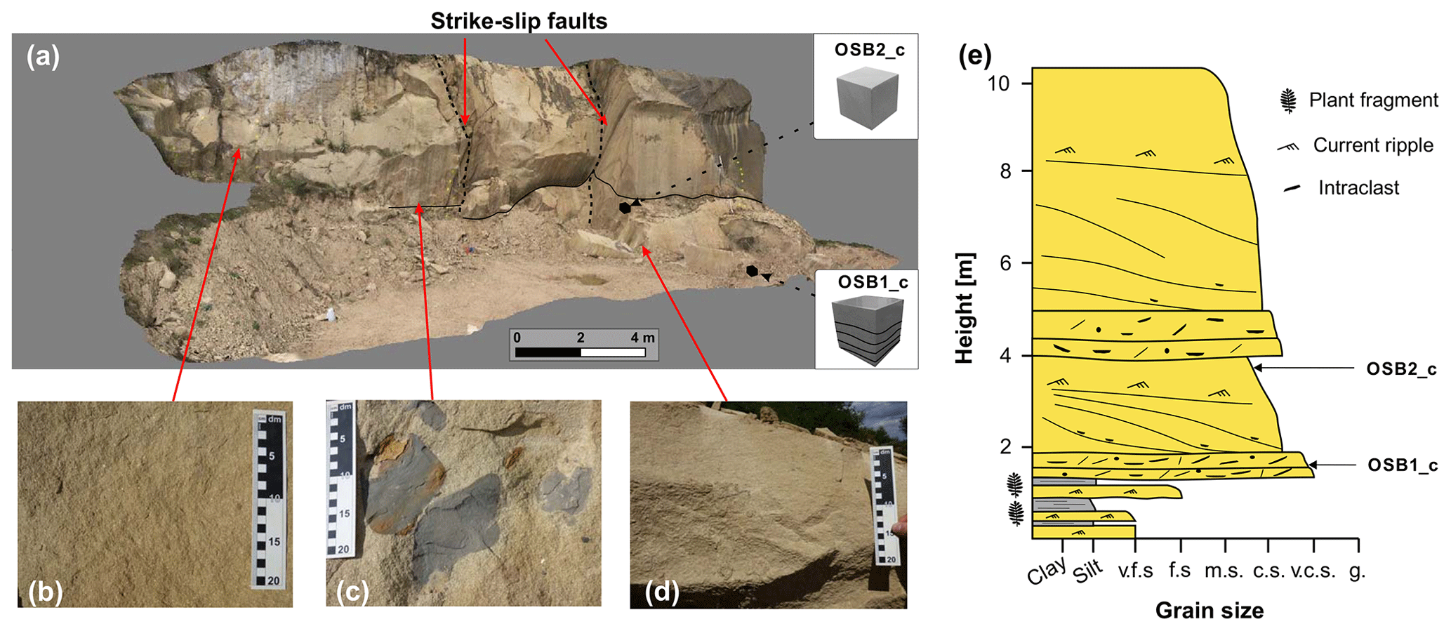
Figure 1(a) The investigated sandstone quarry in Obersulzbach, Germany. The outcrop is compartmentalized in the central part by two strike-slip faults which belong to the Lauter fault zone (Stollhofen, 1998). The strike-slip faults provide offsets of a few meters. (b) Massive sandstone. (c) Pelitic rip-up clasts embedded in a massive rock matrix. (d) Ripple-cross bedded sandstone. (e) Cumulative sedimentary log of the outcrop architecture. The sampling positions of OSB1_c and OSB2_c are marked in the sedimentary log (v.f.s. – very fine sand; f.s. – fine sand; m.s. – medium sand; c.s. – coarse sand; v.c.s. – very coarse sand; and g. – granule).
Two rock cubes of m (OSB2_c) and m (OSB1_c) were extracted from the outcrop wall using a rock chainsaw. According to the outcrop's coordinate system, one edge of the cuboid runs east–west (x), one north–south (y) and one in an altitudinal (z) direction. The irregular cuboids were reworked to regular cubes with a stationary rock saw. We selected two types of lithofacies (Fig. 1e) – both sandstones – with one representing a heterogeneous, compartmentalized variety (OSB1_c) and the other one being a homogeneous variety (OSB2_c). The cubes were both extracted from a distributary mouth bar that is building a foreset in a fluviatile-dominated lacustrine delta. OSB1_c (Fig. 2) was taken from the high energetic basal part, whereas OSB2_c was taken from the lower energetic top. The sedimentological characteristics, including grain size, sorting, angularity, sedimentary structures and mineral content, were determined by visual inspection, thin section and ESEM analyses. Two different types of zonal anisotropy and spatial patterns were expected to be found with the aforementioned sampling strategy. In other studies, such as McKinley et al. (2011), measurements were directly conducted in the field. This approach, however, often provides a drawback with the accuracy and precision, especially in permeability measurements. In order to address this issue, we performed analyses on the faces of the cubes under laboratory conditions. In the next step, the cubes were cut into rock slabs from which cylinder samples were extracted. In total, 108 rock cylinders – 79 from OSB1_c and 29 from OSB2_c – were extracted from the rock cubes. It was ensured that at least five samples were produced that were representative for each Cartesian direction. By applying the formula for calculating a cylinder's volume Vc with the following:
where h is the height of the cylinder and r the radius, the relative volume covered by the rock cylinders in the rock cubes was calculated to be 25.4 % for OSB1_c and 18.2 % for OSB2_c, respectively. Eventually, target meshes are needed to interpolate the full 3D scalar fields. Therefore, both cubes were modeled in 3D using a regular grid consisting of 27 000 hexahedral orthogonal cells. The elementary cell of OSB1_c has a volume of m3, whereas OSB2_c's elementary cells have a volume of m3.
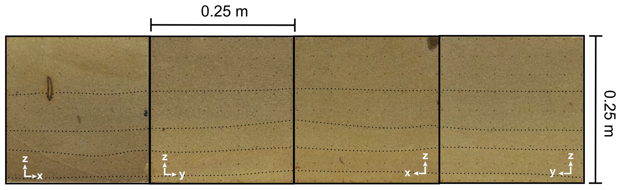
Figure 2Lateral faces of OSB1_c displayed in the form of an open cube (from left to right: XZ front, YZ front, XZ back and YZ back). The internal bounding surfaces are indicated by the dotted lines.
2.2 Laboratory experiments
First, a local metric coordinate system was defined, where each edge of the cube represents an axis in the Cartesian coordinate system in order to reference each measurement to a point in space. The sampling points were set in a raster of 9×9 points on each face for OSB1_c and 5×5 for each face of OSB2_c. All measurements were conducted in the laboratory of the Institute of Applied Geosciences in Darmstadt, Germany. After drying the rock cubes at 60 ∘C, noninvasive measurements were conducted on each face of the cube. On the cubes' faces, the P-wave and S-wave velocity and elemental mass fractions were determined (Fig. 3).
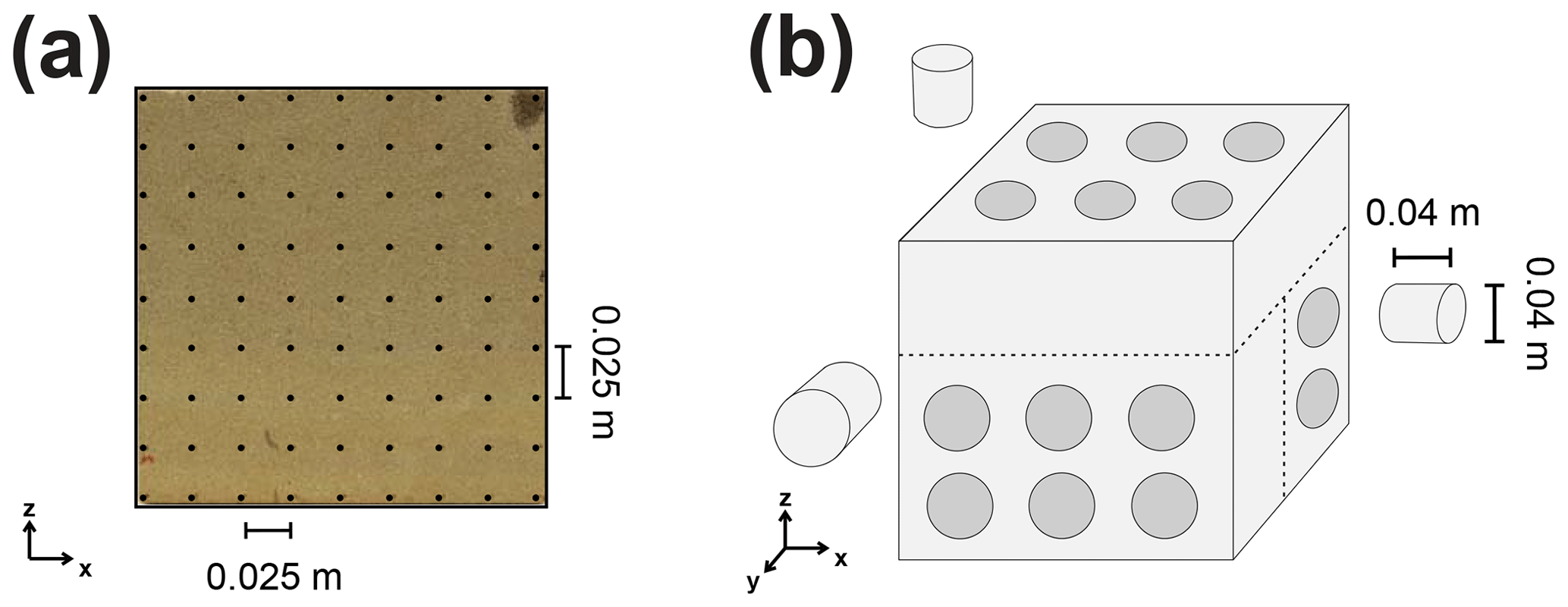
Figure 3(a) Sampling locations for the noninvasive measurements, including P-wave and S-wave velocity and X-ray fluorescence, displayed for the face XZ back of OSB1_c. (b) Schematic of the extraction strategy for sampling the rock cylinders.
After the extraction, the rock cylinders were ovendried at 105 ∘C and measured in order to determine the intrinsic gas permeability, effective porosity, P-wave and S-wave velocity, elemental mass fractions, thermal conductivity, and the thermal diffusivity in unsaturated conditions. Those properties can be considered key properties of the rock matrix in porous aquifers with regard to hydrothermal systems (Agemar et al., 2014) since they constitute input variables for the governing equations for heat transfer and fluid flow in the subsurface (Carslaw and Jaeger, 1959).
The permeability was measured with the Hassler cell permeameter, which is described in Filomena et al. (2014). The Hassler cell is a gas-driven permeameter which measures the permeability of a cylinder-shaped rock sample under steady-state gas flow. This technique allows for the estimation of the intrinsic gas permeability, which is the permeability at an infinite pressure gradient. The permeameter was set to accept a measurement if 15 consecutive readings did not deviate by more than 5 %. The measurement error, however, can exceed that value, especially in low permeable lithologies. Effective porosity measurements were conducted using an envelope density analyzer (GeoPyc 1360). The accuracy is given by the manufacturer to be within ±0.55 % (Micromeritics, 1998). Thermal properties under unsaturated conditions, namely the thermal conductivity and thermal diffusivity, were determined with a thermal conductivity scanner (TCS) according to the work of Popov et al. (1999). The measurement error is quantified to be ≤3 % for thermal conductivity and ≤8 % for thermal diffusivity (Popov et al., 1999). The elastic properties of P-wave and S-wave velocity in the rock media were measured with the sonic wave generator UKS-D (Geotron Elektronik) by sending a sonic wave pulse from a pulse-providing test head (UPG-S) to a receiver (UPG-E). The wave velocity is a function of the travel length and time, together with the density of the material. The initial occurrence of the P wave or S wave must be picked manually after visual inspection by the operator. Thus no measurement error can be provided since user bias cannot be assessed quantitatively. Bulk elemental analysis using the Bruker S1 TITAN handheld portable X-ray fluorescent (pXRF) analyzer was used to find correlations between the elemental composition and the petrophysical properties. The measurement device works on the basis of energy-dispersive X-ray fluorescence (EDXRF) and estimates the elemental mass fractions of a sample. This device produces an ionizing X-ray beam with a diameter of 1.2 cm and quantifies the elemental composition based on the energy emitted by the ionized elements in the targeted area. The portable device can measure the fraction of elements with an ordinal number ≥12 and ≤235 if the threshold value, defined by the measurement error for the specific element in the sample, is exceeded. For this study, the device was operated in GeoChem, Dual Mining mode, allowing for the detection of the major oxides of SiO2, Al2O3, Fe2O3 and K2O and a wide range of other elements. The device was calibrated with international standards. We used the previously mentioned major oxides for analyses since those can provide insight into the iron oxide and clay mineral distribution, which can significantly impact the petrophysical properties. More details on the measurement devices can be found in the works of Hornung and Aigner (2002), Sass and Götz (2012), Filomena et al. (2014), and Aretz et al. (2015).
2.3 Data analysis and spatial modeling
2.3.1 Variography
The experimental semivariogram represents the cumulative dissimilarity of a discrete set of point pairs x, with nc as the count of point pairs within the distance classes h of identical distance increments (Eq. 2).
The continuous counterpart, represented by the variogram model, is an approximation of the experimental semivariogram that assumes z(x) to be a stationary random field (Wackernagel, 2003). A variogram model γtheo is represented by a covariance function c, with the relationship , where c is a positive definite even function. Six covariance models are mostly used to fit the experimental semivariogram, namely the spherical, gaussian, exponential, power, cardinal sine and the linear model (Armstrong, 1998; Ringrose and Bentley, 2015). In this study, we only observe spherical relationships with a nugget effect. This model is calculated as follows:
with the variables nugget (n), range (a) and sill (b). Semivariograms can be used to quantify the spatial or time correlation of a random property (Ringrose and Bentley, 2015; Gu et al., 2017; Rühaak et al., 2015). Further on, the differences in range and sill in dissimilar directional semivariograms can quantify the zonal and geometric anisotropy of a property (Ringrose and Bentley, 2015). The resulting covariance function is an input variable for geostatistical interpolation algorithms.
2.3.2 Rock property interpolation
Spatial inter- and extrapolation can be generated with deterministic and geostatistical techniques. All interpolations are based on the assumption that a point xk with a known value z(xk) has a weight on a discrete point x0 in space with an unknown value z(x0). The global known points, however, can be reduced to a local neighborhood of x0.
For deterministic interpolation, the p value inverse distance weighting (IDW; Shepard, 1968) interpolation is used. The IDW interpolation generally calculates an unknown value z(x0) at point x0 by weighting the distance of that point to each known value point (xk) in space. The underlying formula for IDW is as follows:
where d is the Euclidean distance between the point with the known value xk and the point with the unknown value x0, and p is an exponent factor to bias the weights nonlinearly. The p value is mostly used for smoothing the results by controlling the distance decay effect (Lu and Wong, 2008). IDW is a reliable and widely applied method to interpolate static rock properties in a 1D to 3D space (Rühaak, 2006).
For geostatistical interpolation, simple kriging (SK) is used. Kriging in general is a popular technique for interpolating geological properties in space (Goovaerts, 1997; Rühaak, 2015; Malvić et al., 2019). Through kriging, the value z(x0) at an unknown point x0 is calculated by weighting the neighboring known values and building a linear combination of those via the following formula:
where wk is the weight of the known point xk with the value z(xk). SK requires knowledge of the stationary mean μ (Deutsch and Journel, 1998), which modifies Eq. (5) into the following:
To obtain the simple kriging weights, a set of n equations has to be solved. This set of equations can be written as follows:
with c as the covariance function and xn as the point with a known value (Wackernagel, 2003). The quality of kriging interpolation is dependent on the variogram model, defined neighborhood, sampling density and goodness of fit to the experimental values.
2.4 Cross validation
Cross validation can be used to assess the quality of a model. During cross validation, p randomly selected samples are removed from the input data set of size n with , and the interpolation is performed without those samples (Celisse, 2014). The measures of goodness of fit being used in this study include the root mean square error (RMSE) as follows:
and the mean absolute error (MAE) as follows:
with as estimated value at point xk. Those parameters allow for the quantitative assessment of an interpolation's quality. They might be prone to bias if the sampling density in the target domain is extremely scarce.
2.4.1 Anisotropy
Anisotropy describes the dependence of a physical property on a direction. Rock properties such as stiffness, permeability or thermal conductivity are anisotropic in most cases. Hence, measurements of those properties might show differing magnitudes in different directions if the medium is polar anisotropic. The intrinsic permeability, for example, provides typical ranges for the ratio between the vertical (kv) and horizontal permeability (kh) of 10−5 to 1 (Ringrose and Bentley, 2015). Anisotropy in geological media is generated by the preferred orientation of mineral grains or cracks and by the intrinsic anisotropy of single crystals (Thomsen, 1986).
In the following, we will provide an exemplary description of the anisotropy of elasticity, and we will provide measures for anisotropy quantification under the simplifying assumption of transverse isotropy. The elastic modulus tensor can be expressed as a fourth rank tensor as follows:
where Cij represents an elasticity modulus and the indices are related to the directional P-wave and S-wave velocity, under the assumption that z is the symmetry axis. The velocities can be calculated by the following:
where vp is the P-wave velocity and vs is the S-wave velocity parallel to the symmetry axis and ρ is the bulk density (Yang et al., 2020). The anisotropy, here exemplarily expressed for the P-wave polar anisotropy, can be quantified with the Thomsen parameters (Thomsen, 1986). For example, ϵ can be expressed as follows:
If ϵ≪1, the material can be classified as weakly anisotropic.
2.4.2 Correlation and regression analysis
In order to quantify the linear statistical relationship between two independent variables x and y, the Pearson linear product–moment correlation coefficient (R) can be used. R is expressed as follows:
with n representing the number of compared point pairs and and standing for the arithmetic mean of x and y.
Regression aims at finding a fitting function between samples of two or more random variables. For curvilinear regression, a function of a degree > 1 will be approximated for a discrete set of values. A second-degree polynomial function f(x), for instance, would be described as follows:
Thus, we would need to find n+1 regression coefficients, where n is the degree of f(x). In general, the regression model yields the following:
with . The regression coefficients bm are obtained through solving a system of linear equations as follows:
where x and y are the samples. The function approximations, as produced in regression analyses, are commonly evaluated by the coefficient of determination (R2), which is calculated through the following:
where
is the explained sum of squares, and
is the total sum of squares.
2.4.3 Spatial modeling and statistical analyses
The spatial dependence of the discrete values is evaluated through experimental semivariograms. The semivariograms are generated for the single rock faces, where measurements are available, and for the plug measurements. The empirical semivariogram is fitted to a variogram model, which is then used for the geostatistical interpolation. Interpolation analyses are performed as IDW and SK realizations (Fig. 4) that are assessed through cross validation. The power parameter for IDW is chosen to be three since this constant provides the lowest RMSE among the realizations. The search radii for each prediction is chosen to be 0.2 m, in x and y direction, and 0.15 m, in z direction, in OSB1_c to account for the sedimentary structures. For OSB2_c, the search radii are chosen to be isotropic with a length of 0.2 m. To make the methods comparable, we selected the maximum number of neighboring points to be 25 to represent between 5 % and 95 % of the measurements.
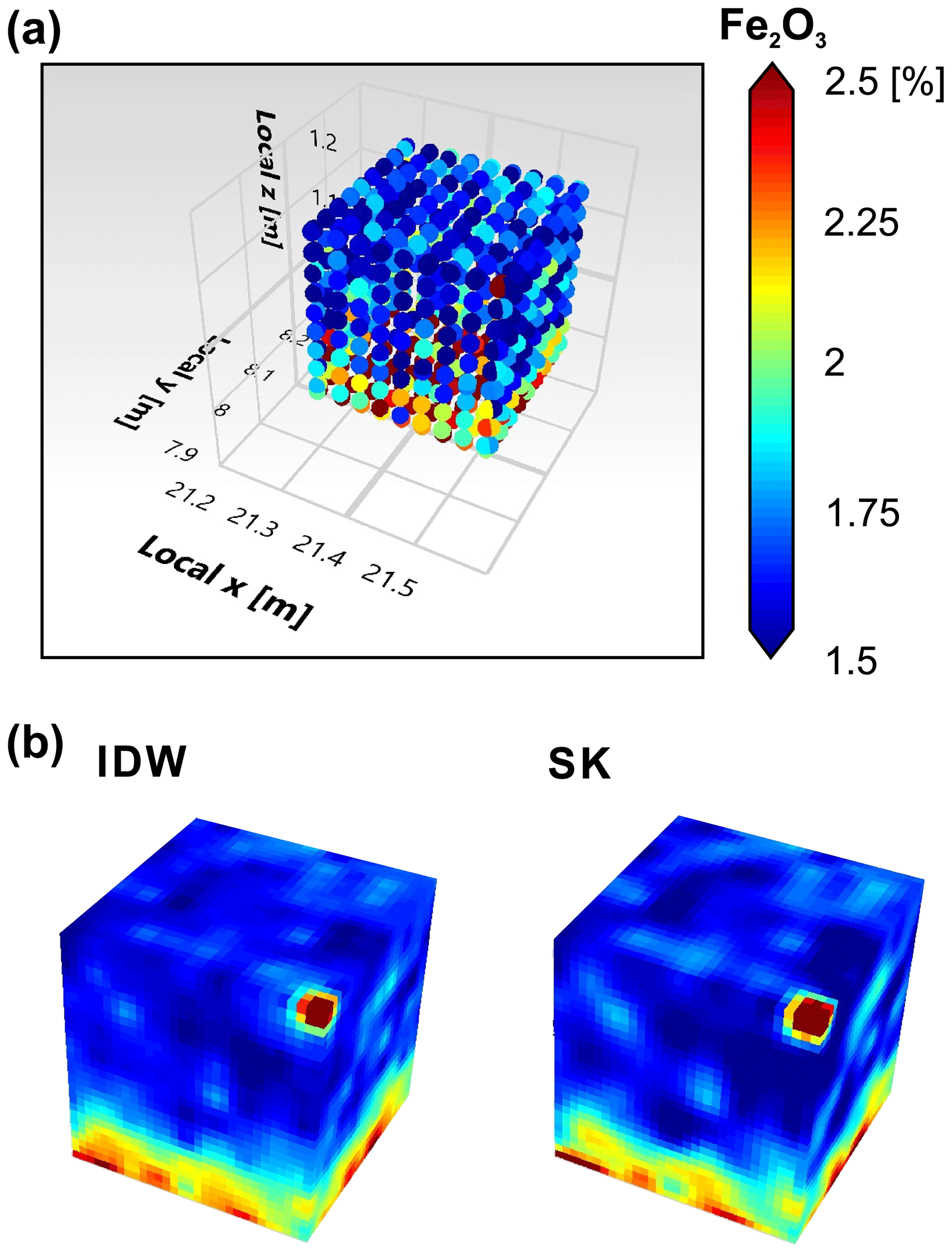
Figure 4(a) Fe2O3 measurement locations on the cube faces of OSB1_c and on the rock samples extracted from the cube. The diameter of one point is 1.2 cm, which corresponds to the beam diameter of the pXRF measurement device. (b) Visual representation of the inverse distance weighting (IDW) and simple kriging (SK) realization of the 3D scalar field of Fe2O3, using the discrete points displayed in (a) as known data points.
We decided to waive sequential simulation as large amounts of the cubes' volumes are covered by rock samples. Thus, we do not expect a relevant kriging variance. With this in mind, the simulations are assumed to capture most of the total variance from the measurements themselves. The interpolation results that provide the lowest cross validation error are used for statistical analyses in order to derive correlations and regression functions between the scalar fields. Eventually, significant correlations are compared with the noninterpolated data sets. Both the spatial modeling and the statistical analyses are performed with the open source software called Geological Reservoir Virtualization (GeoReVi; Linsel, 2020a). This software tool provides functionality for multidimensional subsurface characterization using the concept of knowledge discovery in databases, which is helpful when handling huge data sets such as those produced in this study.
3.1 Sedimentological characteristics
The sandstones belong to a clinothem strata deposited in a fluvial-dominated lacustrine delta. More specifically, the architectural element represents a distributary mouth bar formed by rapid sandstone deposition in sheet-like bodies, as described in Fongngern et al. (2018). The base of those bodies is typically erosive, which is why muddy rip-up clasts commonly occur above the base. Also, the beds, which deposited after the intraclast-rich basal beds, typically show trough or ripple-cross stratification with set heights of 5–15 cm. The vertical orientation of rip-up clasts can be observed in matrix-rich debrites or turbidites deposited under high-energy turbulent hyperpycnal to homopycnal flow conditions (Li et al., 2017). Those are unconformably overlying lacustrine, laminated mud strata from the prodelta environment. Accordingly, Bouma A–E layers (Bouma, 1962; Middleton, 1993) with a prograding trend can be identified in the outcrop. With ongoing sedimentation, the depositional energy in a Bouma sequence typically decreases, which leads to massive sandstones. OSB1_c was taken from a basal bed of the Bouma A interval characterized by a high number of rip-up intraclasts, normal grading and subhorizontal pseudolayering, which may occur in a Bouma A interval if the rip-up clasts experienced buoyancy during transport. OSB2_c was taken from the topmost bed, which corresponds to a Bouma E interval that is characterized by a massive structure.
The average grain size in both cubes ranges from fine to very coarse sand (200–1400 µm). While the grain size distribution in OSB2_c does not show a significant variability – mainly characterized by medium to coarse sand – a normal grading is observable in OSB1_c. Here, the grain size gradually decreases from very coarse sand at the base to medium sand at the top. Likewise, sorting increases from poor to moderate. In OSB2_c the sorting is moderate throughout the entire sample volume. The components provide a low to medium sphericity, while the grain shapes vary between subangular and subrounded. Locally, pelitic rip-up clasts occur with diameters of up to 4 cm. The rip-up clasts show a very low textural maturity and are subvertically oriented with respect to bedding.
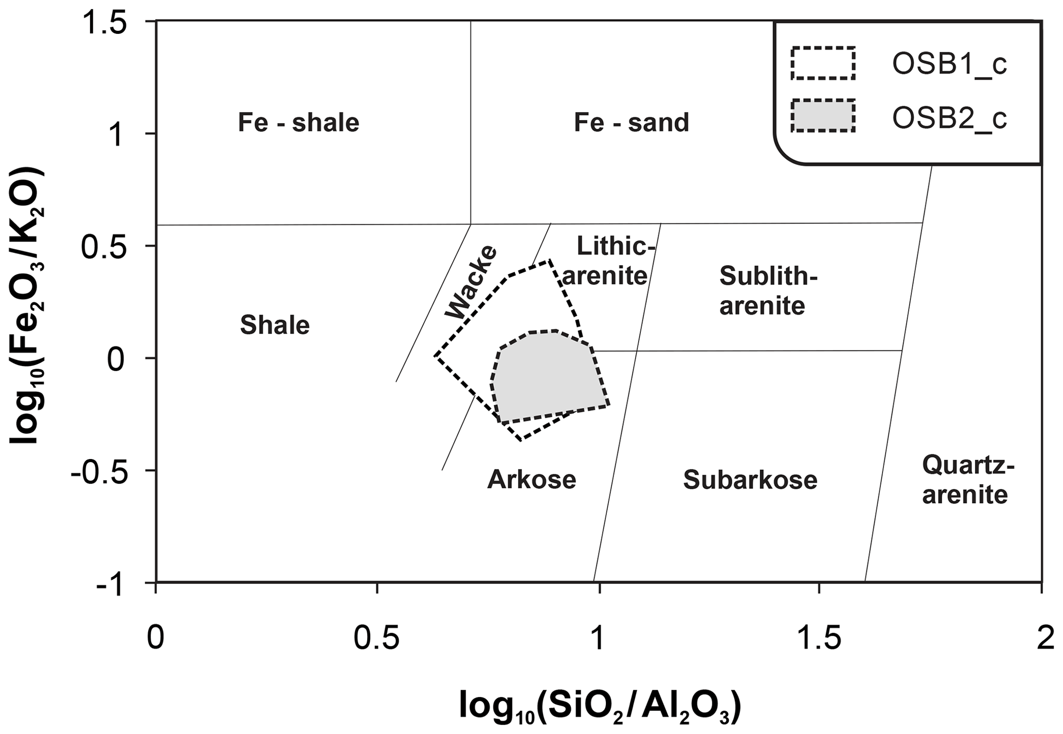
The original rigid detrital components consist of 50 %–60 % quartz, 20 %–30 % strongly altered feldspar and 10 %–25 % lithic fragments. Mica grains are often bent between more rigid grains. The rock matrix accounts for approximately 10 %–20 % and is built up by detrital grains, coated by iron oxides, ductile, autochthonous pelite grains and fine-grained quartz. According to the geochemical analyses, the rocks can be classified as lithic arenites to arkoses or wackes (Fig. 5), respectively, if the matrix content exceeds 15 % based on the classification of Herron (1988).
Thin section analysis (Fig. 6a) reveals that most of the pore space is secondary due to grain dissolution. The secondary pores are undeformed, indicating that grain dissolution took place during structural inversion – probably during telogenesis, according to the concept of Worden and Burley (2003). Most of the primary intergranular volume was destroyed during mechanical compaction. ESEM analysis (Fig. 6b) confirms the presence of quartz accompanied by coprecipitated calcite, opaque phases – mainly iron oxides – and authigenic clay minerals including kaolinite and illite in the cement fraction. Thus, chemical compaction had taken place due to iron oxide, quartz and clay mineral precipitation during diagenesis. Here, the earliest cement phase is represented by the opaque phases comprising a high number of iron oxides. Thereafter, kaolinite is formed, mainly in the secondary pore space, and overgrown by illite. Often, the early cement is overgrown syntaxially by quartz. The source of SiO2 might be internal and related to feldspar dissolution.
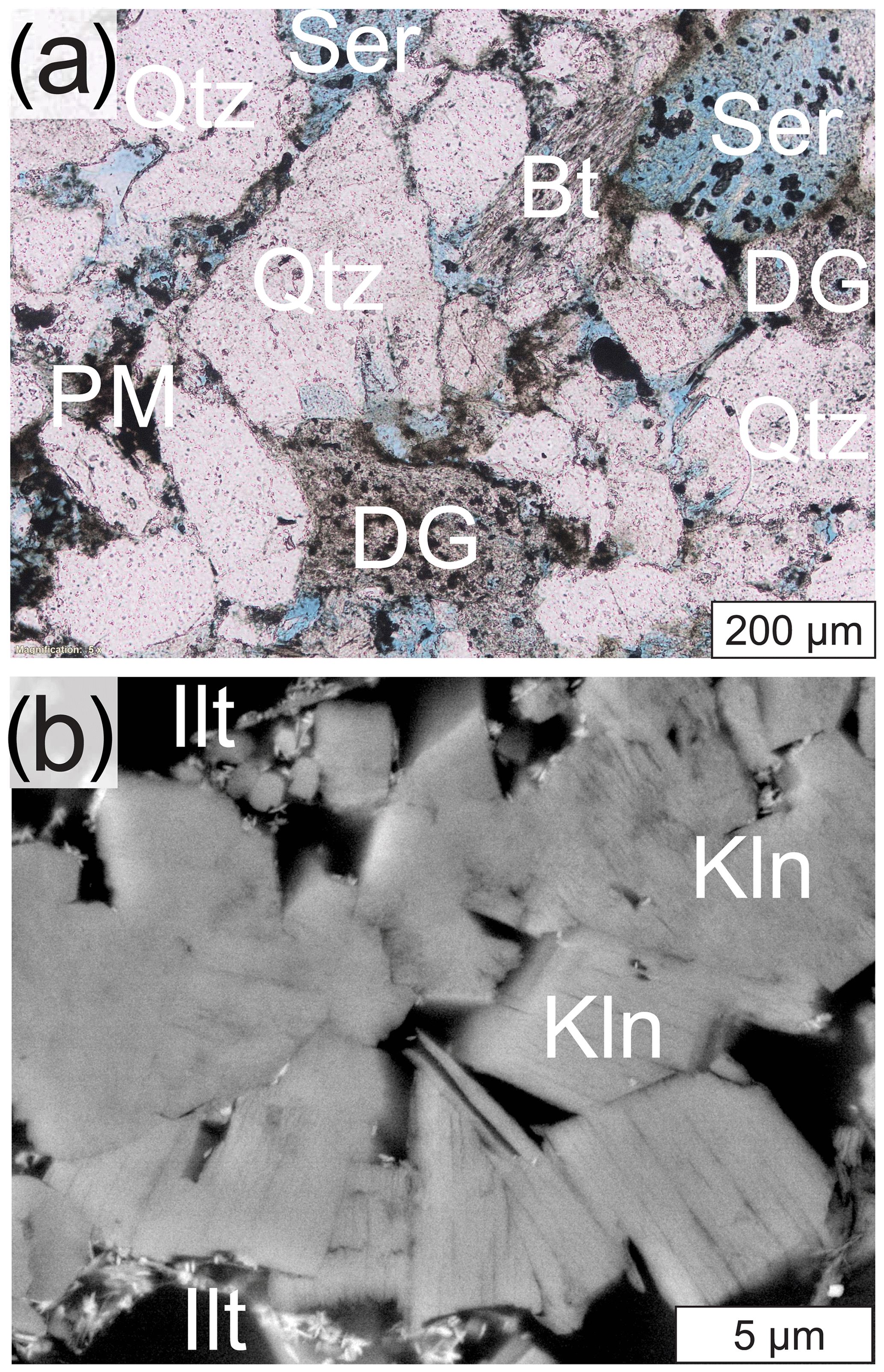
Figure 6(a) Representative thin section taken from rock cube OSB2_c. The sandstone consists mainly of quartz (Qtz), altered feldspars with residual mineral aggregations (sericite – Ser), altered biotite (Bt) and ductile grains (DG). Feldspar dissolution lead to a high grade of secondary porosity (Molenaar et al., 2015), while the vast majority of the intergranular pore space is filled with primary and pseudomatrix (PM) which is rich in iron oxides. (b) Environmental scanning electron microscope (ESEM) image of the authigenic clay minerals, mainly kaolinite (Kln) and illite (Ilt), built in the pore space. Mineral abbreviations were taken from Whitney (2010).
3.2 Exploratory data analysis
In order to provide full comparability, the following section will provide an overview of the measurements derived from the rock cylinder analyses. For each property, 79 rock samples from OSB1_c and 29 from OSB2_c were investigated. An overview of the rock properties' ranges is provided in the box and whisker charts shown in Fig. 7.

Figure 7Box and whisker charts showing the empirical distribution of the rock properties measured in the rock cylinders taken from the rock cubes. Outliers were detected according to Tukey's method (Tukey, 1977), where a value is tested to be in the 1.5 times interquartile range of the arithmetic mean. (a) Intrinsic permeability – k. (b) Effective porosity – ϕ. (c) P-wave velocity – vp. (d) S-wave velocity – vs. (e) Thermal conductivity – λ. (f) Thermal diffusivity – α; the mass fraction of (g) silicon oxide – SiO2. (h) Iron oxide – Fe2O3. (i) Aluminum oxide – Al2O3. (j) Potassium oxide – K2O.
The local variability of OSB1_c is significantly higher than that of OSB2_c. The intrinsic permeability of OSB1_c provides a coefficient of variation of 0.3 and a Dykstra–Parsons coefficient of 0.4, while measurements from OSB2_c show values of 0.2 for the coefficient of variation and 0.18 for the Dykstra–Parsons coefficient, respectively. According to the classification provided by Corbett and Jensen (1992), the intrinsic permeability of both rock cubes can be classified as being very homogeneous. Also, the intrinsic permeability does not show a significant anisotropy.
The range of values in OSB1_c for each property is greater than the range of those in OSB2_c. OSB1_c provides lower values in P-wave and S-wave velocity, thermal conductivity and mass fraction of Fe2O3 compared to OSB2_c. Intrinsic permeability and porosity, in turn, are greater. The mass fraction of silicon oxide and thermal diffusivity provides similar statistical parameters in both cubes; however, the ranges are marginally larger in OSB1_c. The measurements of the elastic rock properties revealed a weak anisotropy of the P-wave attenuation, especially in rock cube OSB2_c. The Thomsen parameter ϵ is 0.047 for OSB1_c and 0.096 for OSB2_c. It should be noted that OSB1_c provides visible bedding structures in contrast to OSB2_c; hence, the observed degree of anisotropy is not connectable to the bedding features in this case.
Statistically significant linear correlations (Fig. 8), in the sense of passing a two-tailed significance test at the 0.05 level, were found between porosity and permeability, permeability and Fe2O3, vp and vs, vp and SiO2, vp and Al2O3, vp and K2O, Fe2O3 and SiO2, and K2O and Al2O3. The strongest positive linear correlation can be observed between vp and vs (R=0.88), K2O and Al2O3 (R=0.70), and porosity and permeability (R=0.31). The strongest negative correlation can be observed between permeability and Fe2O3 (). Properties not being mentioned do not provide significant statistical correlations to others.

Figure 8Matrix visualization of the Pearson correlation coefficient derived from the plug measurements. Statistically significant correlations with a p-value ≤ 0.05 are highlighted by gray boxes. The diameter of the ellipses' conjugate axes is dependent on the correlation coefficient. The smaller the length of the axis, the stronger the correlation. The matrix is diagonal, meaning that the Pearson correlation coefficient as numerical expression is located at the diagonal position relative to each ellipsis. Φ – effective porosity; k – permeability; λ – thermal conductivity; α – thermal diffusivity; vp – P-wave velocity; and vs – S-wave velocity.
3.3 Submeter-scale spatial correlation
The spatial dependence of the discrete measurements is estimated using experimental semivariograms. Therefore, the geochemical representatives SiO2 (Fig. 9a) and Fe2O3 (Fig. 9b) that were measured on each of the rock faces of OSB1_c are given an exemplary analysis. The experimental semivariograms greatly vary from rock face to rock face in OSB1_c. The nugget effect for each experimental variogram is very low. The range of each semivariogram varies between 0.05 and 0.3 m. In the experimental semivariograms of SiO2, two types of patterns can be identified. The XY base, XZ back and YZ front of the rock faces show ranges of approximately 0.08 m and a sill between 8 %2 and 10 %2, until the semivariance exponentially increases when exceeding a lag distance of 0.2 m. The semivariance on the other rock faces runs similarly, with ranges of 0.2 m and a sill of 4.7 %2. The semivariogram for Fe2O3 shows some similarities. Here, the XY base, YZ front and XZ front of the rock faces show very low ranges between 0.05 and 0.15 m and a sill between 0.1 %2 and 0.15 %2 again, with an exponential increase when exceeding a lag distance from 0.2 to 0.25 m. In contrast, the semivariance of YZ back has the highest sill, with 0.21 %2 and a range of 0.15 m; however, semivariance drops after exceeding a lag distance of 0.2 m. XZ back provides the highest degree of similarity with a range of 0.3 m and a sill of 0.09 %2, using a spherical approximation. Both geochemical properties show a zonal anisotropy where the sill shows different magnitudes along different directions (Wackernagel, 2003; Allard et al., 2016).
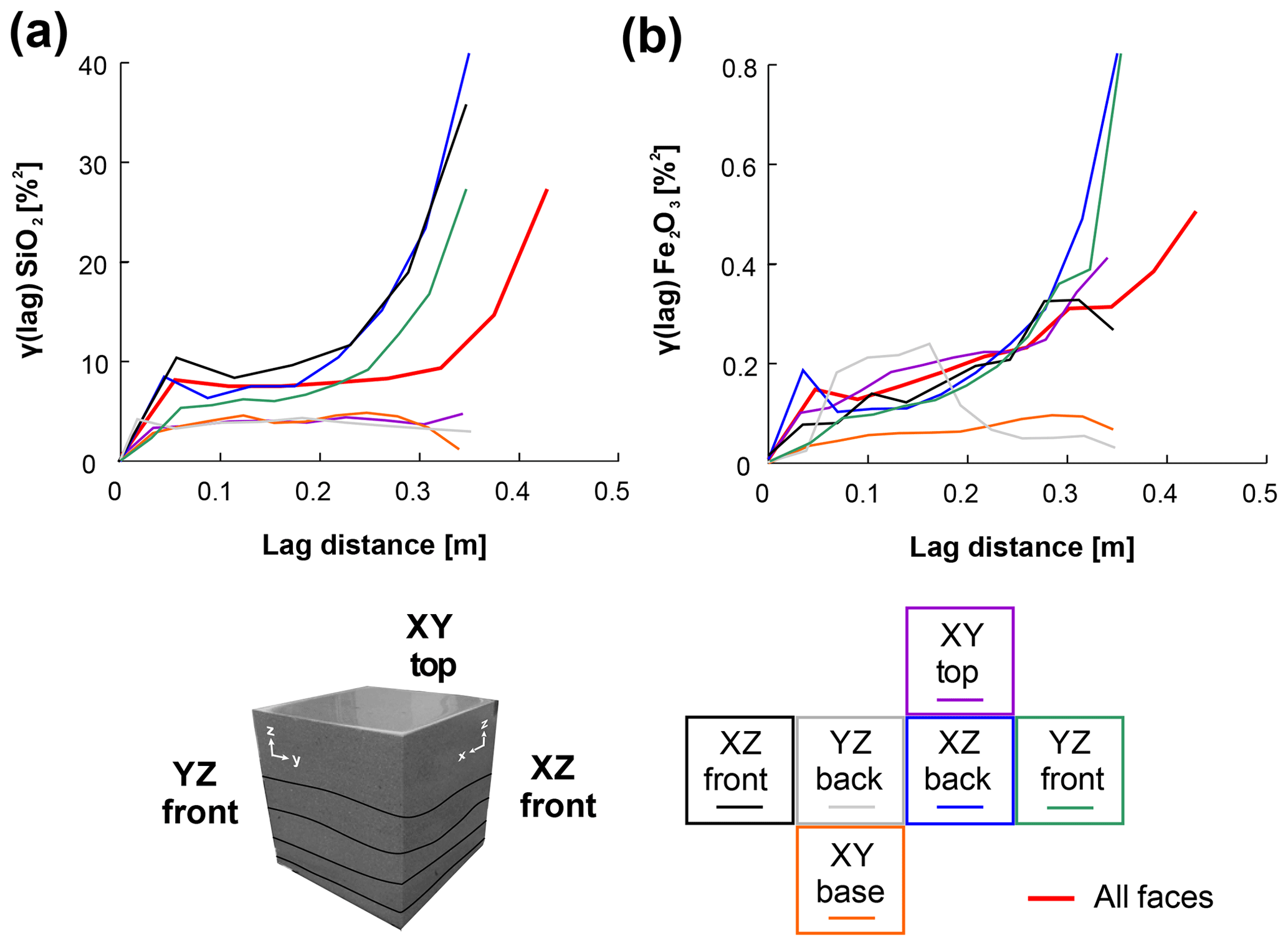
Figure 9Empirical semivariograms of the mass fraction of SiO2 (a) and Fe2O3 (b) in rock cube OSB1_c grouped by the investigated rock face.
3.4 Spatial pattern analysis
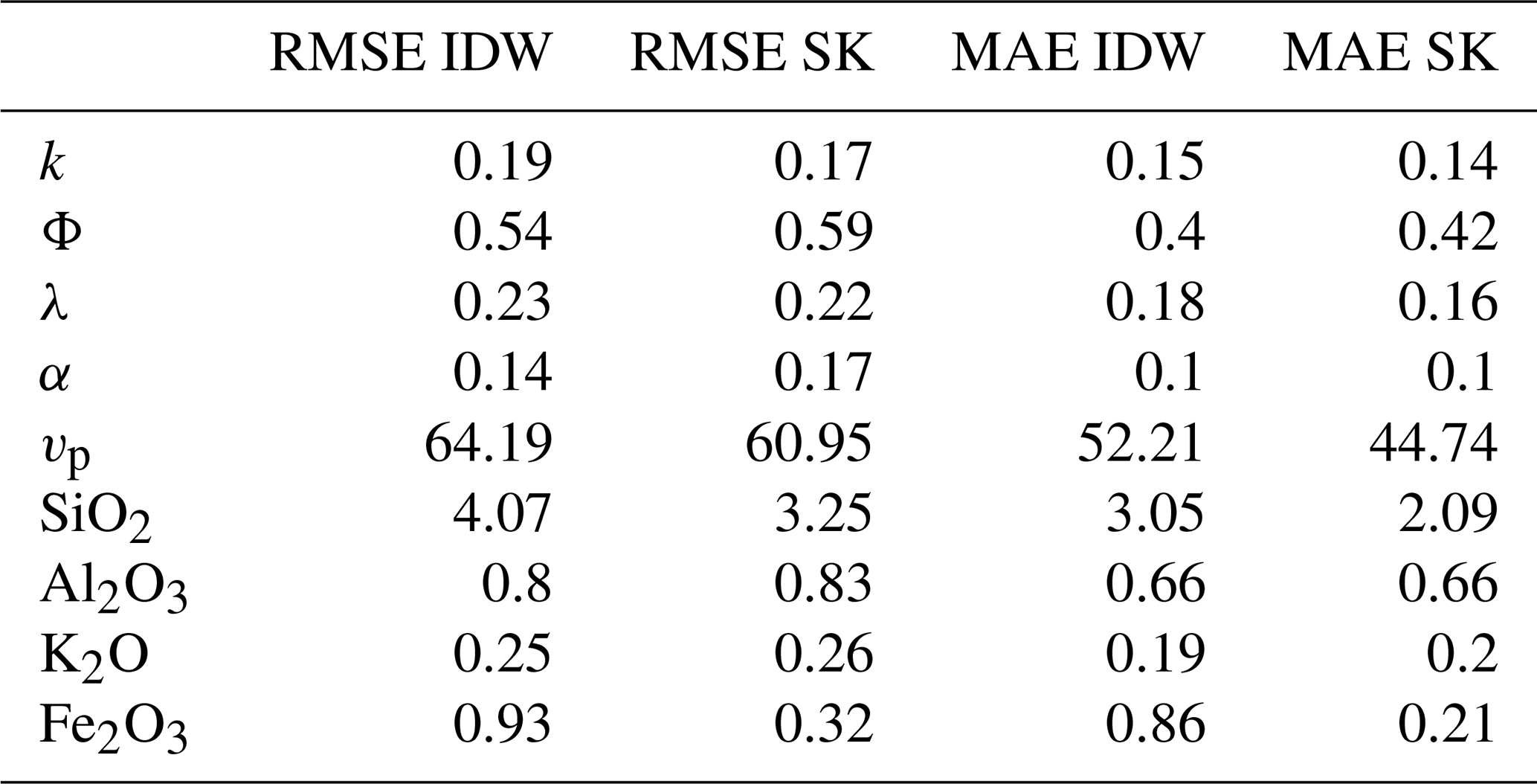
The spatial distributions of the rock properties are interpolated with Shepard's inverse distance weighting (IDW) and simple kriging (SK). Both realizations of a single scalar field provide comparable patterns, which is due to the high sampling density. The interpolation errors are also located in similar ranges; however, IDW seems to be more sensitive to outliers, resulting in much higher interpolation errors with regard to properties like P-wave velocity or mass fraction of SiO2 (Table 1). IDW tends to underestimate the maximum and minimum values in the scalar fields. Thus, petrophysical and geochemical contrasts are more distinctly reproduced in the geostatistical approach. Also, the IDW realization shows the bull's eye effect, which is a typical artifact of IDW interpolations (Shepard, 1968). Accordingly, the simple kriging realizations are used for further analyses.
The rock properties exhibit a multitude of spatial patterns. Here, discrete, layered and homogeneous patterns, both connected and disconnected to primary sedimentary structures, could be observed in the interpolations.
Table 1RMSE and MAE for the interpolation results of IDW and SK for OSB1_c. k – permeability; Φ – effective porosity; λ – thermal conductivity; α – thermal diffusivity; and vp – P-wave velocity.
3.4.1 Patterns connected to sedimentary structures
A bedding-connected pattern is exhibited in the intrinsic permeability and Fe2O3 interpolation results of OSB1_c. The mass fraction of Fe2O3 varies between 1.25 % and 5 % in OSB1_c. In the histogram displayed in Fig. 11, outliers were removed according to Tukey's outlier-detection method (Tukey, 1977). The local histogram of OSB1_c's intrinsic permeability shows a bimodal distribution ranging from 0.7 to 3.9 mD. The application of Tukey's method revealed no statistical outliers in this scalar field.
The bedding structures in OSB1_c are well reflected by the spatial pattern of the interpolated intrinsic permeability gradually increasing from low values, between 0.7 and 2 mD, in the lower beds to higher values, between 2 and 4 mD, in the upper beds (Fig. 10).
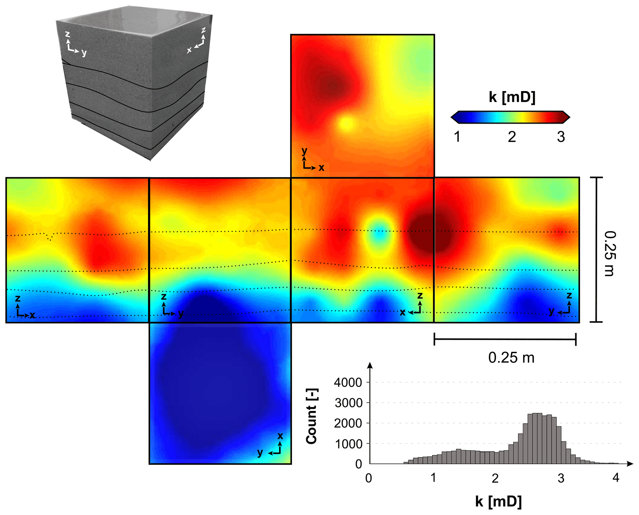
Figure 10Spatial distribution of the intrinsic permeability modeled with a simple kriging interpolation. The histogram shows a bimodality of the distribution split up into the basal beds and uppermost beds.
The spatial distribution of the mass fraction of Fe2O3 in OSB1_c provides a reciprocal trend compared to the permeability. Here, the lowermost bed shows a significantly higher content compared to the upper beds. Both scalar fields show zonal anisotropy. The Fe2O3 content is an indicator of the detrital matrix, pseudomatrix and cement content that, in turn, would explain the reciprocal relationship with the permeability measurements. In siliciclastic systems, iron can be contained in clay minerals (up to 30 wt %; Brigatti et al., 2006), mafic components or in iron-rich oxides, hydroxides or carbonates. Local excesses in the Fe2O3 content exist in the spatial distribution. Those can be explained by clay-rich intraclasts observed on the rock faces. When comparing the pattern to Fig. 2 at both XZ-oriented cube faces, rip-up clasts can be observed where high Fe2O3 mass fractions occur. Those areas provide the maximum values of the Fe2O3 distribution.
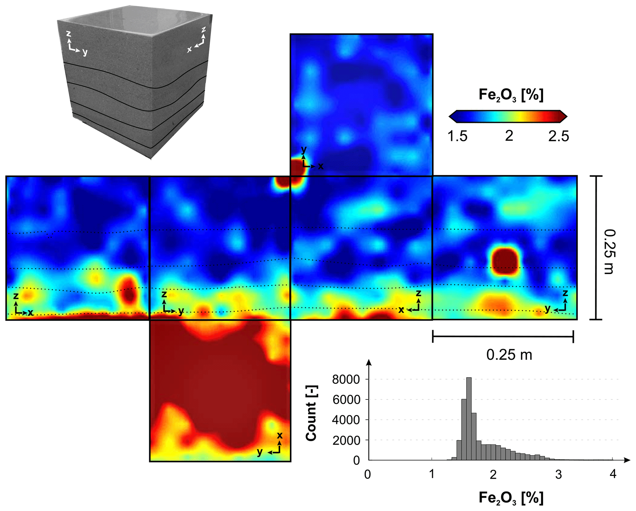
Figure 11Spatial distribution of the mass fraction of Fe2O3 modeled with a simple kriging interpolation. As in the intrinsic permeability interpolation, a bimodality can be observed in the empirical histogram.
3.4.2 Patterns decoupled from sedimentary structures
Other scalar fields are decoupled from depositional bounding surfaces. For instance, the geochemical mass fractions of K2O (Fig. 12) and Al2O3 (Fig. 13) provide a significant positive correlation unconnected to visible structural boundaries. Typically, those geochemical properties are indicative of the presence of orthoclase feldspar (KAlSi3O8) and/or illite (KAl3Si3O10(OH)2) in siliciclastic environments. The mass ratio of both components is roughly 1 : 3 to 1 : 4, which is in accordance to the illite fraction that was observed in the thin section and ESEM analyses. Only minor amounts of orthoclase feldspar could be found in the thin sections. Thus, we assume that the correlation of K2O and Al2O3 can be traced back to the illite phases.
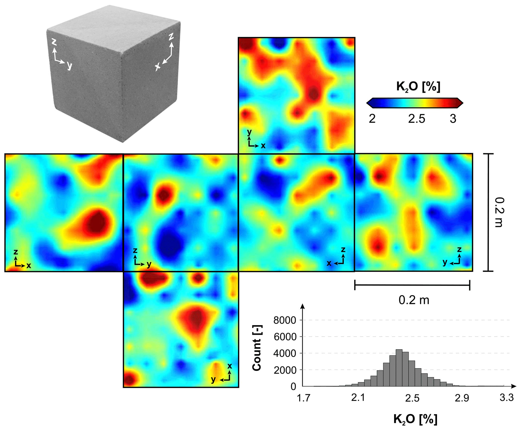
Figure 12Spatial distribution of the mass fraction of K2O modeled with a simple kriging interpolation. The pattern is decoupled from primary sedimentary structures and shows a network-like structure.
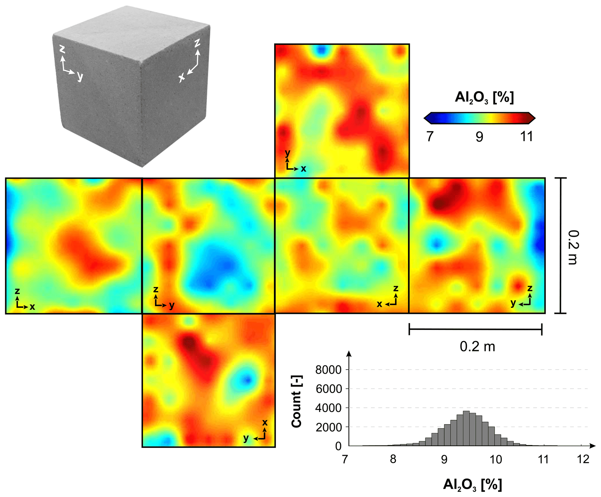
Figure 13Spatial distribution of the mass fraction of Al2O3 modeled with a simple kriging interpolation. The pattern is decoupled from primary sedimentary structures and shows a network-like structure.
Higher fractions of Al2O3 are supposedly due to higher kaolinite (Al2Si2O5(OH)4) fractions in the clay mineral assemblages. The patterns are diffuse, showing autocorrelated areas of slightly enriched and depleted mass fractions. Enriched areas seem to be connected, building network-like patterns, while depleted areas are more isolated.
The overall aim of this study was to quantify the 3D interdependencies of thermophysical, hydraulic, elastic and geochemical scalar fields in sandstone media at the lithofacies scale and to identify the controlling factors for the property distributions. With a high-resolution study at the lithofacies scale, statistical and spatial interrelationships between characteristic physicochemical fields could be discovered and traced back to depositional and diagenetic processes.
4.1 Petrophysical and geochemical characteristics
Recent multiscale modeling approaches without the use of local constraints show that the prediction of permeability and porosity in siliciclastic systems is still challenging (Nordahl et al., 2014). Geological sampling almost never includes the entire domain that is investigated. With sampling densities of 25.4 % and 18.2 %, we reached a very high degree of coverage. Studies such as Hurst and Rosvoll (1991) showed that a very high sampling density is necessary to cover the entire variance of permeability at the lithofacies scale. The interpolations performed in this study reproduce the global histogram properly and outliers are also accounted for. This, in fact, implies that the sampling density was selected adequately in order to capture the total variability present in the physical and geochemical scalar fields. This condition is typically only fulfilled in sequential simulations (Robertson et al., 2006) rather than in conventional interpolations.
Although statistically significant correlations may imply a natural relationship between physicochemical properties, this relationship could also be based on random processes requiring causality to be verified. Weak correlations were found between the effective porosity and the intrinsic permeability, which are usually positively correlated (Pape et al., 1999). This relationship can be traced back to the Kozeny–Carman equation that connects the permeability with the effective pore throat radius and a formation factor F as follows:
The formation factor is defined as the ratio of tortuosity and porosity showing that porosity and permeability provide a positive formal relationship empirically. A high number of secondary pores, produced by feldspar dissolution, did not significantly contribute to the permeability in the investigated sandstones since those pores are often hydraulically isolated. Consequently, secondary porosity did not necessarily lead to increasing radii of the effective pore throats rather than increasing tortuosity. Also, recrystallized quartz cement – blocking a large number of the pore throats – must be taken into account. Both effects, in turn, resulted in a degraded permeability. In addition to the geometrical aspects previously mentioned, the alteration products in the form of clay minerals occupy the pore space, which lead to larger adhesive effects that hinder the ability to transport fluids as well. This observation is in good agreement with observations made by Molenaar et al. (2015) in Rotliegend rocks from the Donnersberg Formation. In addition, these observations are well reflected by the very low values of the intrinsic permeability in both rock cubes. Another reason for the very low intrinsic permeability is the high amount of primary clay and the low maturity of deltaic sheet-like distributary mouth bar deposits (Tye and Hickey, 2001).
The linear correlation analysis revealed a significant negative relationship between hydraulic and geochemical properties that fits to a polynomial regression (Fig. 14). It should be considered that the geochemical measurements cover a very different measurement area – represented by a spot with a 1.2 cm diameter and around 0.5 cm penetration depth compared to the hydraulic measurements performed on an entire rock cylinder with a 40 mm height and diameter. Additionally, instead of using highly precise stationary X-ray fluorescence devices for measurements, a portable, faster device was used to efficiently derive spatial trends in the objects of investigation. This technique weakens the implications for absolute values; however, the trends observed in the measurements from the portable device are in good agreement with trends observed by stationary devices. Also, the observed geochemical characteristics are in accordance with geochemical properties of quartz-rich sandstone varieties that were investigated in Bhatia (1983) or Baiyegunhi et al. (2017).
Geochemical analyses, in contrast to petrographic ones, limit the interpretations of geological processes as mineral phases can only be assumed and not determined for certain. A high mass fraction of Fe2O3 may imply that the rock is rich in iron-bearing minerals like clay minerals, hematite, magnetite, goethite, lepidocrite or ferrihydrite (Costabel et al., 2018), however, a precise classification of the mineral phase is not possible. Iron oxides are more common in secondary precipitates that usually form during eo- and mesodiagenesis (Pettijohn et al., 1987). The degrading impact of iron-oxide-rich coatings on permeability and porosity in unconsolidated sand and gravel has been shown in studies like Costabel et al. (2018). The number of detrital iron-rich phases, such as hematite, which are present in the rock matrix, is typically less (Walker et al., 1981; Turner et al., 1995; Ixer et al., 1979) when compared to the secondary amount. In our case, however, thin section and ESEM analyses revealed that a high degree of the intergranular matrix is still preserved, especially at the base of OSB2_c where high amounts of mud and mud intraclasts are incorporated from basal erosion. The small grain size of the matrix offers a great surface area for iron-oxide-rich precipitates, which might have further enforced degradation of porosity and permeability. The primary matrix typically plugs the pore throats of porous, matrix-rich media. This reduces the ability to conduct fluids compared to matrix-free ones. However, due to progressive compaction, we cannot quantify for certain how large the size of the primary matrix is compared to the pseudomatrix produced by the plastic compaction of ductile, clay-rich grains and by feldspar dissolution.

Figure 14Regression analysis of the relationship between intrinsic permeability and mass fraction of Fe2O3 in the interpolated scalar fields of the rock cube OSB2_c. is the coefficient of determination for the plug measurements, and is the coefficient of determination for the interpolated values.
A significant correlation between K2O and Al2O3 could be detected. The spatial distribution resembles a network-like structure that might be either a product of diffusive mass transport during meso- or telodiagenesis or it might reflect the distribution of feldspar grains and its residues in the sandstone. During feldspar alteration, SiO2 is dissolved and K remains in the alteration products, which could be an implication for the mesoscale network-like structure into which pore fluids could have had migrated. This relationship is underlined by a negative, yet nonsignificant, correlation of K2O with SiO2.
Significant nonintuitive relationships between the physical and geochemical scalar fields at the lithofacies scale have been revealed with a deductive approach of spatial field modeling and statistical data analysis. All in all, the following conclusions can be drawn from this study:
-
As specific properties such as the mass fraction of Fe2O3 preserve sedimentological textures well in their spatial distribution, other properties seem to be completely decoupled from depositional bounding surfaces. These scalar fields probably reflect processes that might have taken place during the diagenetic overprint of the rocks as a result of burial and exhumation. These processes produce diffuse patterns, as discussed with regard to the correlation of K2O and Al2O3.
-
This study demonstrates that the observation of bedding structures does not necessarily indicate a stronger polar anisotropy compared to macroscopically unstructured lithologies. Here, the microscopic characteristics, like the amount of secondary porosity, might play a more important role in the attenuation of physical waves than the bounding surfaces.
-
It could be shown that hydraulic properties are dependent on the intergranular matrix and cement amount, which are in turn controlled by depositional processes and eogenetic precipitates. Those findings are not new (see Wilson and Pittman, 1977 or Nordahl et al., 2014); however, they have not been evaluated in lithofacies-scale 3D environments yet. We assume that primary matrix and ductile grain content has the most detrimental effect on rock permeability. Ductile grains were mechanically deformed during compaction, leading to plugged pore throats. Feldspar dissolution has a highly productive effect on porosity but not on permeability.
-
We demonstrate that the strength of statistical correlation can be preserved in spatial interpolations as long as the sampling density is sufficient. If the sampling density is too low, a statistical correlation might be inadvertently feigned.
-
As shown in this study, the local geological variability should not be underestimated as an uncertainty factor in spatial predictions and upscaling procedures. In fact, the local geological variability of physicochemical properties might nearly cover the variability being present in an entire formation. Therefore, a high-resolution analysis of physicochemical rock properties can assist in assessing the uncertainty of field-scale property models which is induced by the local geological variability at the lithofacies scale.
GeoReVi is an open source software for Windows systems available at https://github.com/ApirsAL/GeoReVi (https://doi.org/10.5281/zenodo.3695815, Linsel, 2020a). The executables are available in the repository at https://github.com/ApirsAL/GeoReVi/blob/master/binaries/ (last access: 11 August 2020). The measurements are available at https://doi.org/10.6084/m9.figshare.11791407.v2 (Linsel, 2020b).
The investigated rock samples are available at the Institute of Applied Geosciences, TU Darmstadt, and can be requested from linsel@geo.tu-darmstadt.de. Also, the samples are registered in the System for Earth Sample Registration (SESAR; http://www.geosamples.org, last access: 11 August 2020; registration numbers are provided in the data set of Linsel, 2020b).
AL conceptualized and prepared the paper. AL and SW conducted the laboratory and field measurements. JH contributed to the conceptualization of the study. MH was the overall supervisor of the study.
The authors declare that they have no conflict of interest.
The authors are grateful for the permission to work in the sandstone quarry of Konrad Müller GmbH in Obersulzbach, Germany. Also, we would like to thank Reimund Rosmann and Institut IWAR (Technische Universität Darmstadt, Germany) for the preparation of the rock cubes. We are extremely thankful to Mattia Pizzati and Giacomo Medici for their time and effort in putting together constructive reviews. Adrian Linsel has received financial support from the Friedrich-Ebert-Stiftung, Germany, which is gratefully acknowledged.
This research has been supported by the Friedrich-Ebert-Stiftung, Germany.
This paper was edited by Kei Ogata and reviewed by Giacomo Medici and Mattia Pizzati.
Agemar, T., Weber, J., and Schulz, R.: Deep geothermal energy production in Germany, Energies, 7, 4397–4416, https://doi.org/10.3390/en7074397, 2014. a
Allard, D., Senoussi, R., and Porcu, E.: Anisotropy models for spatial data, Math. Geosci., 48, 305–328, https://doi.org/10.1007/s11004-015-9594-x, 2016. a
Aretz, A., Bär, K., Götz, A. E., and Sass, I.: Outcrop analogue study of permocarboniferous geothermal sandstone reservoir formations (northern Upper Rhine Graben, Germany): impact of mineral content, depositional environment and diagenesis on petrophysical properties, Int. J. Earth Sci., 105, 1431–1452, https://doi.org/10.1007/s00531-015-1263-2, 2015. a, b
Armstrong, M.: Experimental variograms, Springer, Berlin, Heidelberg, Germany, 47–58, https://doi.org/10.1007/978-3-642-58727-6_4, 1998. a
Baiyegunhi, C., Liu, K., and Gwavava, O.: Geochemistry of sandstones and shales from the Ecca Group, Karoo Supergroup, in the Eastern Cape Province of South Africa: Implications for provenance, weathering and tectonic setting, Open Geosci., 9, 340–360, https://doi.org/10.1515/geo-2017-0028, 2017. a
Becker, A., Schwarz, M., and Schäfer, A.: Lithostratigraphische Korrelation des Rotliegend im östlichen Saar–Nahe–Becken, Jber. Mitt. Oberrhein. Geol. Ver., 94, 105–133, https://doi.org/10.1127/jmogv/94/2012/105, 2012. a
Bhatia, M. R.: Plate Tectonics and Geochemical Composition of Sandstones, J. Geol., 91, 611–627, 1983. a
Bouma, A. H.: Sedimentology of some Flysch deposits; a graphic approach to facies interpretation, Elsevier, Amsterdam, New York, 1962. a
Brigatti, M. F., Galan, E., and Theng, B. K. G.: Chapter 2 Structures and Mineralogy of Clay Minerals, in: Handbook of Clay Science vol. 1, edited by: Bergaya, F., Theng, B. K. G., and Lagaly, G., Elsevier, 19–86, https://doi.org/10.1016/S1572-4352(05)01002-0, 2006. a
Carslaw, H. S. and Jaeger, J. C.: Conduction of Heat in Solids, Second Edition, Oxford University Press, Oxford, United Kingdom, 1959. a
Celisse, A.: Optimal cross-validation in density estimation with the L2-loss, Ann. Stat., 42, 1879–1910, https://doi.org/10.1214/14-AOS1240, 2014. a
Corbett, P. and Jensen, J. L.: Estimating the mean permeability: how many measurements do you need?, First Break, 10, 5, https://doi.org/10.3997/1365-2397.1992006, 1992. a
Corbett, P. W. M., Hamdi, H., and Gurav, H.: Layered fluvial reservoirs with internal fluid cross flow: a well-connected family of well test pressure transient responses, Petrol. Geosci., 18, 219–229, https://doi.org/10.1144/1354-079311-008, 2012. a
Costabel, S., Weidner, C., Müller-Petke, M., and Houben, G.: Hydraulic characterisation of iron-oxide-coated sand and gravel based on nuclear magnetic resonance relaxation mode analyses, Hydrol. Earth Syst. Sci., 22, 1713–1729, https://doi.org/10.5194/hess-22-1713-2018, 2018. a, b
Deutsch, C. V. and Journel, A.: GSLIB: Geostatistical Software Library and User's Guide, Oxford University Press, Oxford, United Kingdom, https://books.google.de/books?id=CNd6QgAACAAJ (last access: 11 August 2020), 1998. a
Filomena, C. M., Hornung, J., and Stollhofen, H.: Assessing accuracy of gas-driven permeability measurements: a comparative study of diverse Hassler-cell and probe permeameter devices, Solid Earth, 5, 1–11, https://doi.org/10.5194/se-5-1-2014, 2014. a, b
Fongngern, R., Olariu, C., Steel, R., Mohrig, D., Krézsek, C., and Hess, T.: Subsurface and outcrop characteristics of fluvial-dominated deep-lacustrine clinoforms, Sedimentology, 65, 1447–1481, https://doi.org/10.1111/sed.12430, 2018. a
Goovaerts, P.: Geostatistics for Natural Resources Evaluation, Oxford University Press, Oxford, United Kingdom, 1997. a
Gu, Y., Rühaak, W., Bär, K., and Sass, I.: Using seismic data to estimate the spatial distribution of rock thermal conductivity at reservoir scale, Geothermics, 66, 61–72, https://doi.org/10.1016/j.geothermics.2016.11.007, 2017. a
Hamdi, H., Ruelland, P., Bergey, P., and Corbett, P. W.: Using geological well testing for improving the selection of appropriate reservoir models, Petrol. Geosci., 20, 353–368, https://doi.org/10.1144/petgeo2012-074, 2014. a
Heap, M. J., Kushnir, A. R. L., Gilg, H. A., Wadsworth, F. B., Reuschlé, T., and Baud, P.: Microstructural and petrophysical properties of the Permo-Triassic sandstones (Buntsandstein) from the Soultz-sous-Forêts geothermal site (France), Geoth. Energy, 5, 26, https://doi.org/10.1186/s40517-017-0085-9, 2017. a
Henk, A.: Mächtigkeit und Alter der erodierten Sedimente im Saar–Nahe–Becken (SW-Deutschland), Geologische Rundschau, 81, 323–331, https://doi.org/10.1007/BF01828601, 1992. a
Herron, M. M.: Geochemical classification of terrigenous sands and shales from core or log data, J Sediment. Res., 58, 9, https://doi.org/10.1306/212F8E77-2B24-11D7-8648000102C1865D, 1988. a, b
Hornung, J. and Aigner, T.: Reservoir Architecture in a Terminal Alluvial Plain: An Outcrop Analogue Study (Upper Triassic, Southern Germany) Part 1: Sedimentology And Petrophysics, J Petrol. Geol., 25, 3–30, https://doi.org/10.1111/j.1747-5457.2002.tb00097.x, 2002. a
Hornung, J., Linsel, A., Schröder, D., Gumbert, J., Ölmez, J., Scheid, M., and Pöppelreiter, M.: Understanding small-scale petrophysical heterogeneities in sedimentary rocks – the key to understand pore geometry variations and to predict lithofacies-dependent reservoir properties, Digital Geology – Multi-scale analysis of depositional systems and their subsurface modelling workflows, Special Volume, EAGE, Houten, the Netherlands, 71–90, ISBN: 9789462823372, 2020. a
Hudson, G. and Wackernagel, H.: Mapping temperature using kriging with external drift: Theory and an example from Scotland, Int. J. Climatol., 14, 77–91, https://doi.org/10.1002/joc.3370140107, 1994. a
Hurst, A. and Rosvoll, K. J.: Permeability Variations in Sandstones and their Relationship to Sedimentary Structures, Academic Press, Inc., San Diego, New York, Boston, London, Sydney, Tokyo, Toronto, 166–196, https://doi.org/10.1016/B978-0-12-434066-4.50011-4, 1991. a, b
Ixer, R. A., Turner, P., and Waugh, B.: Authigenic iron and titanium oxides in triassic red beds: St. Bees Sandstone, Cumbria, Northern England, Geol. J., 14, 179–192, https://doi.org/10.1002/gj.3350140214, 1979. a
Jackson, M. D., Muggeridge, A. H., Yoshida, S., and Johnson, H. D.: Upscaling Permeability Measurements Within Complex Heterolithic Tidal Sandstones, Math. Geol., 35, 499–520, https://doi.org/10.1023/A:1026236401104, 2003. a
Kiryukhin, A. V., Kaymin, E. P., and Zakharova, E. V.: Using TOUGHREACT to Model Laboratory Tests on the Interaction of NaNO3–NaOH Fluids with Sandstone Rock at a Deep Radionuclide Repository Site, Nucl. Technol., 164, 196–206, https://doi.org/10.13182/NT08-A4019, 2008. a
Kushnir, A. R. L., Heap, M. J., Baud, P., Gilg, H. A., Reuschlé, T., Lerouge, C., Dezayes, C., and Duringer, P.: Characterizing the physical properties of rocks from the Paleozoic to Permo-Triassic transition in the Upper Rhine Graben, Geotherm. Energy, 6, 16, https://doi.org/10.1186/s40517-018-0103-6, 2018. a
Lake, L. W. and Srinivasan, S.: Statistical scale-up of reservoir properties: concepts and applications, J. Petrol. Sci. Eng., 44, 27–39, https://doi.org/10.1016/j.petrol.2004.02.003, 2004. a
Landa, J. L. and Strebelle, S.: Sensitivity Analysis of Petrophysical Properties Spatial Distributions, and Flow Performance Forecasts to Geostatistical Parameters Using Derivative Coefficients, Society of Petroleum Engineers, SPE Annual Technical Conference and Exhibition, 29 September–2 October, San Antonio, Texas, https://doi.org/10.2118/77430-MS, 2002. a, b, c
Li, S., Li, S., Shan, X., Gong, C., and Yu, X.: Classification, formation, and transport mechanisms of mud clasts, Int. Geol. Rev., 59, 1609–1620, https://doi.org/10.1080/00206814.2017.1287014, 2017. a
Linsel, A.: GeoReVi v1.0.1, https://doi.org/10.5281/zenodo.3695815, 2020a. a, b
Linsel, A.: Physicochemical Characteristics of Sandstone Media, figshare, https://doi.org/10.6084/m9.figshare.11791407.v2, 2020b. a, b
Lu, G. Y. and Wong, D. W.: An adaptive inverse-distance weighting spatial interpolation technique, Comput. Geosci., 34, 1044–1055, https://doi.org/10.1016/j.cageo.2007.07.010, 2008. a
Malvić, T., Ivšinović, J., Velić, J., and Rajić, R.: Kriging with a Small Number of Data Points Supported by Jack-Knifing, a Case Study in the Sava Depression (Northern Croatia), Geosci., 9, 36, https://doi.org/10.3390/geosciences9010036, 2019. a
McKinley, J. M., Lloyd, C. D., and Ruffell, A. H.: Use of Variography in Permeability Characterization of Visually Homogeneous Sandstone Reservoirs with Examples from Outcrop Studies, Math. Geol., 36, 761–779, https://doi.org/10.1023/b:Matg.0000041178.73284.88, 2004. a
McKinley, J. M., Atkinson, P. M., Lloyd, C. D., Ruffell, A. H., and Worden, R. H.: How Porosity and Permeability Vary Spatially With Grain Size, Sorting, Cement Volume, and Mineral Dissolution In Fluvial Triassic Sandstones: The Value of Geostatistics and Local Regression, J. Sediment. Res., 81, 844–858, https://doi.org/10.2110/jsr.2011.71, 2011. a, b, c, d
McKinley, J. M., Ruffell, A. H., and Worden, R. H.: An Integrated Stratigraphic, Petrophysical, Geochemical and Geostatistical Approach to the Understanding of Burial Diagenesis: Triassic Sherwood Sandstone Group, South Yorkshire, UK, John Wiley & Sons, Inc., Chichester, United Kingdom, 231–255, https://doi.org/10.1002/9781118485347.ch10, 2013. a
Medici, G., West, L. J., and Mountney, N. P.: Characterizing flow pathways in a sandstone aquifer: Tectonic vs. sedimentary heterogeneities, J. Contam. Hydrol., 194, 36–58, https://doi.org/10.1016/j.jconhyd.2016.09.008, 2016. a
Medici, G., West, L. J., and Mountney, N. P.: Characterization of a fluvial aquifer at a range of depths and scales: the Triassic St Bees Sandstone Formation, Cumbria, UK, Hydrogeol. J., 26, 565–591, https://doi.org/10.1007/s10040-017-1676-z, 2018. a
Medici, G., West, L. J., and Mountney, N. P.: Sedimentary flow heterogeneities in the Triassic U.K. Sherwood Sandstone Group: Insights for hydrocarbon exploration, Geol. J., 54, 1361–1378, https://doi.org/10.1002/gj.3233, 2019. a
Miall, A. D.: Architectural-element analysis: A new method of facies analysis applied to fluvial deposits, Earth-Sci. Rev., 22, 261–308, https://doi.org/10.1016/0012-8252(85)90001-7, 1985. a
Micromeritics: GeoPyc 1360 – Envelope Density Analyzer, available at: https://www.micromeritics.com/repository/files/geopyc_1360_reg_and_tap.pdf (last access: 8 August 2020), 1998. a
Middleton, G. V.: Sediment Deposition from Turbidity Currents, Annu. Rev. Earth Pl. Sc., 21, 89–114, https://doi.org/10.1146/annurev.ea.21.050193.000513, 1993. a
Molenaar, N., Felder, M., Bär, K., and Götz, A. E.: What classic greywacke (litharenite) can reveal about feldspar diagenesis: An example from Permian Rotliegend sandstone in Hessen, Germany, Sediment. Geol., 326, 79–93, https://doi.org/10.1016/j.sedgeo.2015.07.002, 2015. a, b
Nordahl, K., Messina, C., Berland, H., Rustad, A. B., Rimstad, E., Martinius, A. W., Howell, J. A., and Good, T. R.: Impact of multiscale modelling on predicted porosity and permeability distributions in the fluvial deposits of the Upper Lunde Member (Snorre Field, Norwegian Continental Shelf), Geol. Soc. Lon., 387, 25, https://doi.org/10.1144/sp387.10, 2014. a, b
Pape, H., Clauser, C., and Iffland, J.: Permeability prediction based on fractal pore‐space geometry, Geophysics, 64, 1447–1460, https://doi.org/10.1190/1.1444649, 1999. a
Pettijohn, F. J., Potter, P. E., and Siever, R.: Mineral and Chemical Composition, Springer New York, New York, NY, 25–67, https://doi.org/10.1007/978-1-4612-1066-5_2, 1987. a
Popov, Y. A., Pribnow, D. F. C., Sass, J. H., Williams, C. F., and Burkhardt, H.: Characterization of rock thermal conductivity by high-resolution optical scanning, Geothermics, 28, 253–276, https://doi.org/10.1016/S0375-6505(99)00007-3, 1999. a, b
Ringrose, P. and Bentley, M.: Reservoir Model Design, First Edition, Springer, the Netherlands, https://doi.org/10.1007/978-94-007-5497-3, 2015. a, b, c, d
Ringrose, P. S., Sorbie, K. S., Corbett, P. W. M., and Jensen, J. L.: Immiscible flow behaviour in laminated and cross-bedded sandstones, J. Petrol. Sci. Eng., 9, 103–124, https://doi.org/10.1016/0920-4105(93)90071-L, 1993. a
Robertson, R. K., Mueller, U. A., and Bloom, L. M.: Direct sequential simulation with histogram reproduction: A comparison of algorithms, Comput. Geosci., 32, 382–395, https://doi.org/10.1016/j.cageo.2005.07.002, 2006. a
Rodrigo-Ilarri, J., Reisinger, M., and Gómez-Hernández, J. J.: Influence of Heterogeneity on Heat Transport Simulations in Shallow Geothermal Systems, Springer International Publishing, Cham, Germany, 849–862, https://doi.org/10.1007/978-3-319-46819-8_59, 2017. a
Rühaak, W.: A Java application for quality weighted 3-d interpolation, Comput. Geosci., 32, 43–51, https://doi.org/10.1016/j.cageo.2005.04.005, 2006. a
Rühaak, W.: 3-D interpolation of subsurface temperature data with measurement error using kriging, Environ. Earth Sci., 73, 1893–1900, https://doi.org/10.1007/s12665-014-3554-5, 2015. a
Rühaak, W., Guadagnini, A., Geiger, S., Bär, K., Gu, Y., Aretz, A., Homuth, S., and Sass, I.: Upscaling thermal conductivities of sedimentary formations for geothermal exploration, Geothermics, 58, 49–61, https://doi.org/10.1016/j.geothermics.2015.08.004, 2015. a
Sass, I. and Götz, A. E.: Geothermal reservoir characterization: a thermofacies concept, Terra Nova, 24, 142–147, https://doi.org/10.1111/j.1365-3121.2011.01048.x, 2012. a
Shepard, D.: A Two-Dimensional Interpolation Function for Irregularly-Spaced Data., in: Proceedings of the 1968 ACM National Conference, Association for Computing Machinery, New York, NY, USA, 517–524, https://doi.org/10.1145/800186.810616, 1968. a, b
Stollhofen, H.: Facies architecture variations and seismogenic structures in the Carboniferous–Permian Saar–Nahe Basin (SW Germany): evidence for extension-related transfer fault activity, Sediment. Geol., 119, 47–83, https://doi.org/10.1016/S0037-0738(98)00040-2, 1998. a
Tellam, J. H. and Barker, R. D.: Towards prediction of saturated-zone pollutant movement in groundwaters in fractured permeable-matrix aquifers: the case of the UK Permo-Triassic sandstones, Geol. Soc. Lon., Special Publications, 263, 1–48, https://doi.org/10.1144/gsl.Sp.2006.263.01.01, 2006. a
Thomsen, L.: Weak elastic anisotropy, Geophysics, 51, 1954–1966, https://doi.org/10.1190/1.1442051, 1986. a, b
Tukey, J.: Exploratory Data Analysis, Pearson, Reading, Massachussetts, USA, 1977. a, b
Turner, P., Burley, S., Rey, D., and Prosser, J.: Burial history of the Penrith Sandstone (Lower Permian) deduced from the combined study of fluid inclusion and palaeomagnetic data, Geol. Soc. Lon., Special Publications, 98, 43–78, https://doi.org/10.1144/GSL.SP.1995.098.01.04, 1995. a
Tye, B. and Hickey, J.: Permeability characterization of distributary mouth bar sandstones in Prudhoe Bay field, Alaska: How horizontal cores reduce risk in developing deltaic reservoirs, AAPG Bull., 85, 459–475, https://doi.org/10.1306/8626C91F-173B-11D7-8645000102C1865D, 2001. a
Verly, G.: Sequential Gaussian Simulation: A Monte Carlo Method for Generating Models of Porosity and Permeability, in: Generation, Accumulation and Production of Europe's Hydrocarbons III, edited by: Spencer, A. M., Springer, Berlin, Heidelberg, Germany, 345–356, 1993. a
Wackernagel, H.: Multivariate Geostatistics, Third Edition, Springer, Berlin, Heidelberg, Germany, https://doi.org/10.1007/978-3-662-05294-5, 2003. a, b, c
Walker, T. R., Larson, E. E., and Hoblitt, R. P.: Nature and origin of hematite in the Moenkopi Formation (Triassic), Colorado Plateau: A contribution to the origin of magnetism in red beds, J. Geophys. Res.-Sol. Ea., 86, 317–333, https://doi.org/10.1029/JB086iB01p00317, 1981. a
Wang, J. and Zuo, R.: Identification of geochemical anomalies through combined sequential Gaussian simulation and grid-based local singularity analysis, Comput. Geosci., 118, 52–64, https://doi.org/10.1016/j.cageo.2018.05.010, 2018. a
Whitney, D. L. and Evans, B. W.: Abbreviations for names of rock-forming minerals, Am. Mineral., 95, 185–187, https://doi.org/10.2138/am.2010.3371, 2010. a
Wilson, M. D. and Pittman, E. D.: Authigenic clays in sandstones; recognition and influence on reservoir properties and paleoenvironmental analysis, J. Sediment. Res., 47, 3–31, https://doi.org/10.1306/212f70e5-2b24-11d7-8648000102c1865d, 1977. a
Worden, R. H. and Burley, S. D.: Sandstone Diagenesis: The Evolution of Sand to Stone, in: Sandstone Diagenesis, edited by: Burley, S. D. and Worden, R. H., 1–44, https://doi.org/10.1002/9781444304459.ch, 2003. a
Yang, J., Hua, B., Williamson, P., Zhu, H., McMechan, G., and Huang, J.: Elastic Least-Squares Imaging in Tilted Transversely Isotropic Media for Multicomponent Land and Pressure Marine Data, Surv. Geophys., 805–833, https://doi.org/10.1007/s10712-020-09588-3, 2020. a
Zheng, S.-Y., Corbett, P. W. M., Ryseth, A., and Stewart, G.: Uncertainty in Well Test and Core Permeability Analysis: A Case Study in Fluvial Channel Reservoirs, Northern North Sea, Norway, AAPG Bull., 84, 1929–1954, https://doi.org/10.1306/8626c72b-173b-11d7-8645000102c1865d, 2000. a