the Creative Commons Attribution 4.0 License.
the Creative Commons Attribution 4.0 License.
 | 26 Aug 2020
Increased density of large low-velocity provinces recovered by seismologically constrained gravity inversion
Wolfgang Szwillus
Jörg Ebbing
Bernhard Steinberger
The nature and origin of the two large low-velocity provinces (LLVPs) in the lowest part of the mantle remain controversial. These structures have been interpreted as a purely thermal feature, accumulation of subducted oceanic lithosphere or a primordial zone of iron enrichment. Information regarding the density of the LLVPs would help to constrain a possible explanation.
In this work, we perform a density inversion for the entire mantle, by constraining the geometry of potential density anomalies using tomographic vote maps. Vote maps describe the geometry of potential density anomalies according to their agreement with multiple seismic tomographies, hence not depending on a single representation. We use linear inversion and determine the regularization parameters using cross-validation. Two different input fields are used to study the sensitivity of the mantle density results to the treatment of the lithosphere. We find the best data fit is achieved if we assume that the lithosphere is in isostatic balance.
The estimated densities obtained for the LLVPs are systematically positive density anomalies for the LLVPs in the lower 800–1000 km of the mantle, which would indicate a chemical component for the origin of the LLVPs. Both iron-enrichment and a mid-oceanic ridge basalt (MORB) contribution are in accordance with our data, but the required superadiabatic temperature anomalies for MORB would be close to 1000 K.
- Article
(5348 KB) - Full-text XML
-
Supplement
(441 KB) - BibTeX
- EndNote


Seismology has systematically revealed more and more of the heterogeneity in the mantle. Interpretations of seismic images often aim at determining the density of features, because buoyancy is the driver of mantle dynamics. For instance, much research has focused on tracing sinking slabs in order to understand how subduction works (e.g. van der Meer et al., 2018). At greater depths such interpretation becomes more difficult, due to reduced resolution and lack of corroborating surface evidence. The most striking features of the lowermost mantle are probably the large low-velocity provinces (LLVPs) (Garnero et al., 2016).
The two LLVPs are antipodal regions of decreased seismic velocity that extend from the core–mantle boundary about 400–800 km into the mantle and cover about 25 % of the surface of the core–mantle boundary (Garnero et al., 2016). There is considerable debate regarding their nature and origin, with them being interpreted as a purely thermal feature (Koelemeijer et al., 2017), an accumulation of subducted oceanic lithosphere (Mulyukova et al., 2015) or iron-enriched zones (Ballmer et al., 2015; Deschamps et al., 2012). In addition, it has been suggested that plumes are formed preferentially at the edges of the LLVPs, based on the reconstructed locations of large igneous provinces and kimberlites (Burke et al., 2008; Conrad et al., 2013), which imply that the LLVPs are stable over long time periods.
The debate regarding the LLVPs is often centred on their density, because density allows one to distinguish between a purely thermal and a thermo-chemical origin. However, direct determinations of density using seismological and geodetic methods have led to contradictory results, indicating either positive (Ishii and Tromp, 1999; Lau et al., 2017; Moulik and Ekström, 2016; Trampert et al., 2004) or negative (Koelemeijer et al., 2017) density anomalies, with a strength between 0.5 % and 2.0 %.
Combining seismology and gravity to investigate the mantle is a well-established approach that typically includes dynamical modelling of mantle convection (Richards and Hager, 1984; Hager and O'Connell, 1979). Most commonly, seismic velocity anomalies are directly converted into density anomalies, and the vertical viscosity distribution is adjusted in order to fit the geoid (Richards and Hager, 1984). Using this technique, many models of viscosity and density inside the mantle have been derived (King, 1995, 2016; Steinberger, 2007, 2016; Richards and Hager, 1984; Hager et al., 1985).
While viscosity inversions can successfully explain the geoid with variance reductions of 80 % or more (King and Masters, 1992; Ricard et al., 1993), this approach relies on some assumptions that can be challenged. To derive a conversion factor from velocity to density anomalies based on mineral physics, often purely thermal anomalies are assumed (Karato, 1993). However, differences in terms of composition certainly play a role in the upper mantle/lithosphere (Griffin et al., 2009) and have been suggested for the lower mantle as well (Ballmer et al., 2017; Deschamps et al., 2012). For example, the velocity and density model Gypsum (Simmons et al., 2009) allows for a partial decorrelation of velocity and density.
Furthermore, the modelled geoid associated with a certain density distribution is partly based on the dynamic topography caused by this density distribution. Thus, viscosity inversion should also reproduce surface topography, since it is an important part of the total gravity effect. However, before the dynamic predictions can be compared to real topography, the isostatic part of topography must be removed using crustal models. While the agreement between predicted and non-isostatic topography has been increasing (Flament et al., 2013; Steinberger, 2016), there are still considerable differences (Molnar et al., 2015).
The justification for directly inverting for density instead of going through viscosity is that the gravity field is only affected indirectly by the viscosity distribution, through viscosity's influence on the deformation of the boundaries (surface and core–mantle boundary) (Hager and O'Connell, 1979). However, the gravity effect of any deformed boundary is independent of what caused the deformation. Thus, the gravity effect of the top boundary (i.e. topography) can simply be calculated and removed from the observed data, without needing any dynamic simulations or viscosity structures. In contrast, the core–mantle boundary (CMB) topography is not well known. While a variety of seismological techniques can be used to estimate CMB topography, there is no consensus regarding amplitude and patterns (see comparisons in Tanaka, 2010). Geodynamical simulations have shown that CMB deformation is sensitive to possible lateral viscosity variations in the lowermost mantle and the viscosity and density variations related to the presence post-perovskite (Deschamps et al., 2018; Deschamps and Li, 2019). Hence, CMB deformation cannot be accounted for a priori, but its possible effects must be considered a posteriori in the interpretation.
In this contribution, we explore an alternative approach for fitting the gravity field using mantle density structure. Instead of density–velocity conversion, we use tomographic vote maps (Lekic et al., 2012; Shephard et al., 2017) to provide geometrical constraints for a linear gravity inversion. The geometry is defined by the fast and slow zone derived from the vote maps, and each zone is assigned an unknown but constant density anomaly. These density anomalies are completely free parameters that are adjusted to fit the gravity field. As input data we use satellite gravity data, corrected for topography and lithosphere. For the latter correction we compare two different approaches. In the first approach it is assumed that the lithosphere is in perfect isostatic balance, and in the second we make use of a recently developed crustal model by Szwillus et al. (2019).
2.1 Gravity data
We use satellite gravity data from the global gravity field model GOCO05S (Pail et al., 2010) at the measurement height (225 km) of the GOCE satellite in its last mission phase (van der Meijde et al., 2015). Often, gravity data are mathematically downward continued to a lower height, but this introduces omission errors (Bouman et al., 2013), which we would like to avoid. In addition, the target density distributions are at such a great depth that downward continuation probably provides no additional sensitivity.
As a first step we calculate an ice-corrected Bouguer anomaly based on the topography of ETOPO1 (Amante and Eakins, 2009). Onshore we assume a density of 2670 kg m−3, and offshore we use a correction density of 1770 kg m−3 based on a reference crustal density of 2800 kg m−3 and a water density of 1030 kg m−3. In addition, the influence of ice is removed assuming a density of 917 kg m−3.
Since we are interested in the mantle density structure, the second step is to account for the gravity effect of the crust and/or lithosphere. Two inherently different approaches exist to achieve this. The first option is to assume some form of isostatic compensation and use this to account for the crust and/or lithosphere. Alternatively, the gravity effect of crustal models, such as Crust1.0 (Laske et al., 2013) or Litho1.0 (Pasyanos et al., 2014) can be calculated. The latter approach includes more geophysical data, but it also “propagates” errors of the crustal model into the mantle. In particular, all crustal models predict several kilometres of residual topography, even in the continents (Steinberger, 2016) and are thus not nearly in isostatic balance. As a consequence, the topography would need to be supported dynamically, which should lead to higher free-air anomaly values than observed (Molnar et al., 2015).
In light of this discrepancy, we explore two approaches. In the first approach, we assume that continental topography is compensated by crustal thickness variations, whereas ocean floor depth is compensated by variations in the mantle lithosphere density (the same isostatic model as in Szwillus et al., 2016, with a compensation depth of 120 km). The isostatic residual is then
where FA is the free-air anomaly (Fig. 1a), gtopo is the gravity effect of topography and giso is the gravity effect of the isostatic compensation masses.

Figure 1Input data for the inversions. (a) Free-air anomaly at a measurement height of 225 km. (b) Isostatic residual gravity anomaly at 225 km height. This is obtained by correcting for the presence of topography and isostatic compensation masses. (c) Crustal residual gravity anomaly at 225 km height obtained by removing the gravity effect of the crustal model from Szwillus et al. (2019). (d) Residual topography after removing the isostatic contribution of the crustal model from Szwillus et al. (2019).
In the second approach, we use our recent crustal model based on kriging (Szwillus et al., 2019) and assume a density contrast between crust and mantle of 400 kg m−3 to estimate the gravity effect of varying crustal thickness. This gives the crustal residual:
where gcrust is the gravity response of the crustal thickness variations.
The isostatic residual is very similar to the free-air anomaly (Fig. 1b), except in areas of high topography. In contrast, the crustal residual has a much higher amplitudes and patterns (Fig. 1c). For comparison we also computed the residual (non-isostatic) topography of the kriging crustal model (Szwillus et al., 2019), which anti-correlates with the crustal residual on large scales (Fig. 1d).
2.2 Geometry constraints
Additional constraints are required to overcome the inherent non-uniqueness of a density inversion. We use information from whole mantle seismic tomographies in the form of vote maps (Shephard et al., 2017) to define volumes which could potentially contain density anomalies. Vote maps were first introduced by Lekic et al. (2012) in the context of cluster analysis and then further developed by Shephard et al. (2017). A vote map is based on a collection of tomography models, and at each point it gives the number of tomographies that detect a significant anomaly at that location. The threshold that constitutes a significant anomaly is the standard deviation at that depth for each seismic tomography. Thus, even tomographies with vastly different amplitude ranges can be combined in a single vote map. We used the vote maps based on 17 S-wave tomography models as available on SubMachine (Hosseini et al., 2018) at a resolution of 1∘ and 100 km depth spacing. There are two separate vote maps for positive and negative anomalies. Figure 2 shows an example of the vote maps at a depth of 2700 km, close to the core–mantle boundary.
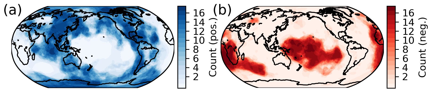
Figure 2Vote maps at 2700 km depth. (a) Vote map for fast (positive) anomalies. (b) Vote map for slow (negative) anomalies. Note the clear signature of the two LLVPs underneath Africa and the central Pacific.
The first step is to discretize the inversion problem by extracting regions of potential density anomalies from the vote map individually for each depth. Our underlying assumption is that density anomalies only occur in horizontally connected regions where at least N tomographies detect anomalous velocity. We choose N=10, because this is the cut-off that correlates with the strongest gradients of the vote maps. Each connected region is assigned a constant but unknown density anomaly. As a result of this process, we have a total of 1135 anomalous regions that are each described in terms of their depths, their pixels and unknown density anomaly values. These density anomalies are completely free parameters that will be adjusted during the inversion to fit the gravity field. Importantly, we impose no correlation between velocity and density.
2.3 Cross-validation inversion approach
Our inversion is a two-step approach. First, we forward calculate for each potential density anomaly region its characteristic gravity response. Second, the characteristic gravity responses of all of the potential density anomalies are placed into a matrix A and solved with a generalized Tikhonov regularization technique. The regularization parameters are chosen based on cross-validation.
The gravity effect of each potential density anomaly is estimated by approximating it as a collection of point masses. Each point mass represents a volume V, given by
where r is the radius, lat is the latitude, Δϕ is the angular size of each pixel (1∘) and Δz is the vertical resolution (100 km). The mass m is then found by multiplying the volume with the density anomaly ρ.
The gravity kernel K(P,Q) caused by a unit point mass located at on a measurement point is given by
where γ is the great-circle distance between the point mass and the measurement point, and m3 (kg s2)−1 is the gravitational constant. The total gravity effect of each potential density anomaly is then found by summing over the gravity effect of all its pixels.
Next, the gravity response of all of the potential density anomalies are placed into a matrix A, where Aij is the gravity effect of potential density anomaly j on measurement point i, assuming a density of 1. Using Eq. (4), Aij becomes
where ℛj is the set of indices belonging to potential density anomaly j; P contains all subsurface points and Q all measurement points.
The unknown density values of the potential density anomalies are placed in a vector ρ. In principle, , where gi=g(Qi) is the measured gravity value at point Qi. However, in practice the solution will be unstable and non-unique, so that regularization is required. Here, we choose to minimize the following least-squares functional:
The three terms relate to the data misfit, the magnitude of density variations and the vertical derivative of density anomaly. is the quadratic form related to matrix M, and is the Euclidean norm. β and γ are the regularization parameters that enforce the minimization of absolute norm of the density anomalies and their vertical derivative respectively. In addition, the parameter β represents the ratio of data variance to model variance. D is a finite differencing matrix consisting of first-order forward vertical differences in density. Finally, Matrix Σg is an assumed correlation matrix of the gravity values. We use an isotropic correlation function with a correlation distance of 10∘, based on a semivariogram analysis (Chilès and Delfiner, 2012). The main purpose of the matrix is to down-weigh observation points near the pole, which are otherwise over represented due to convergence near the pole.
The optimal ρ belonging to this formulation is
The regularization parameters β and γ exert critical control over the resulting density structure and the achievable data fit. The most popular methods to determine such parameters are L curves and cross-validation (Farquharson and Oldenburg, 2004). Here we use cross-validation to estimate the regularization parameter.
In k-fold cross-validation, the gravity data set is randomly split into k distinct index sets ℐj. The first set ℐ1=𝒯 then becomes the training set and the remaining sets are combined to form the validation set 𝒱. The training set is then used to solve the inversion problem giving a solution ρ1. Based on how well ρ1 predicts the data in 𝒯 and 𝒱, the training and validation misfit is calculated. Each ℐ𝒿 becomes the training set once, and this is repeated for many random partitions of the data.
By design, the training misfit is minimal when β and γ are zero (if there are no numerical instabilities). However, small values of β and γ also risk overfitting the data. By carrying out cross-validation for all combinations of β and γ in a reasonable range of values, the optimal β and γ corresponding to the minimum validation misfit can be found.
Apart from constraining the regularization parameters, this procedure also gives a bootstrap estimate (Efron and Gong, 1983) of the density structure. The collection of all the density anomaly estimates derived for all subsets of gravity data can be used to calculate a mean density anomaly value and its standard deviation for each potential anomaly, given certain regularization parameters. This is useful to determine how robust a single density anomaly is.
2.4 Boundary topography
The surface and CMB deformations implied by the density model recovered by inversion are important to judge the quality of the results. The surface topography predicted by the density model should roughly agree with the residual topography, because topography is strongly sensitive to density. The magnitude of the CMB deformation is required to assess how much it affects the gravity field fitting.
We determine the deformation of the upper and lower domain boundary caused by density structure as a postprocessing step after inversion. We use both an isostatic and a simple dynamic formulation to determine this deformation.
Let tCMB(lat,long) be the CMB-topography as a function of longitude and latitude. Under the assumption of isostatic balance at the CMB, we find
where ΔρCMB is the density jump at the CMB, H is the height above the CMB where isostatic balance applies, and is the mean density between r=CMB and .
We convert the density difference associated with undulating topography into a surface density σ=tCMBΔρCMB and calculate its gravity response in spherical harmonics by
where values are the spherical harmonic coefficients of the surface density, is a spherical harmonic function and km is the radius of the observations.
Isostatic surface topography is calculated in the same way using the upper 300 km of the domain and a density contrast of 2670 kg m−3 at the surface.
To determine the dynamic surface and CMB topography we use the propagator matrix approach of Hager and O'Connell (1979), with free slip boundary conditions on the surface and CMB. The viscosity is layered and increases by a factor of 100 at 700 km depth. This is a simplification of the real viscosity structure, which is additionally affected by lateral variations due to temperature and – possibly – compositional differences.
The resulting kernels show that for the assumed viscosity structure, the influence of density anomalies below 500 km on topography is limited, even at very long wavelengths (Fig. 3a). The CMB kernels decrease much more slowly, even with a layered viscosity (Fig. 3b) and even at degree 10.

Figure 3Topography and CMB kernels calculated using the propagator matrix approach (Hager and O'Connell, 1979). The black line is computed using a two-layer viscosity structure, the grey line uses a constant viscosity. The solid line is for spherical harmonic degree 2 and the dashed line for spherical harmonic degree 10.
3.1 Inversion using isostatic residual
A grid search of β and γ values between 10−3 and 103 using the cross-validation procedure leads to a minimum validation misfit of 5.32 mGal if β=0.03 and γ=1.0 (Fig. 4a). Although this minimum is not particularly well developed, we proceed with these values of β and γ, since neighbouring regularization settings give similar results. With these regularization parameters, the training misfit becomes 3.25 mGal, which is about 20 % of the rms of the input gravity field (96 % variance reduction).
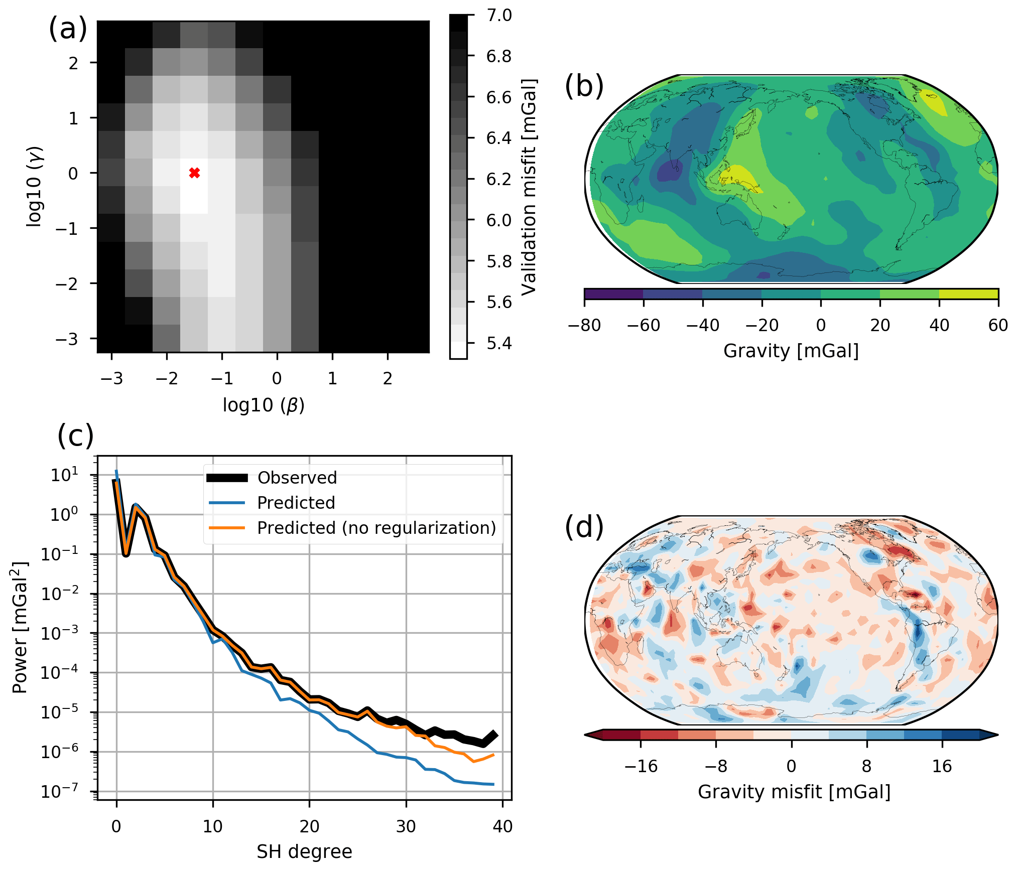
Figure 4Results of the inversion using the isostatic residual. (a) Validation misfit as a function of regularization parameter β. (b) Predicted field of the inversion results. (c) Spectral comparison of the input and predicted data. (d) Difference between input and predicted data.
The inversion is able to reasonably reproduce the main features of the isostatic residual gravity field (Fig. 4b). However, the amplitude of the residual field is systematically too small. A linear regression of the gravity field predicted from the model against the measured values gives a linear factor of 0.85, implying that the modelled anomalies are about 15 % too weak. This is probably a result of the regularization.
In the spectral domain, the predicted gravity field is able to reproduce the long-wavelength part up to spherical harmonic (SH) degree 10 (Fig. 4c). At shorter wavelengths, the predicted field is systematically too weak, going down to less than 10 % of the observed data at spherical harmonic degree 40. For comparison, the solution with no regularization () is able to reproduce the spectrum up to spherical harmonic degree 25 perfectly. Thus, wavelengths shorter than SH degree 25 simply cannot be produced, due to the insufficient spectral content of the vote maps.
The inverted density anomalies show no clear correlation with sign of the velocity anomaly (Sect. 4.2), which would suggest that many density anomalies are not caused only by temperature variations. The spatial distribution is highly complex, and not all density anomalies are easily related to expected features. However, some first-order trends can be identified (Fig. 5).

Figure 5Density anomaly slices through selected depths of the inversion results using the isostatic residual.
The upper 100 km of the inversion results contain very little density variations (Fig. 5a). Some cratons (South America, South Africa, Eurasia) show a slight negative density anomaly (Fig. 5b). This is probably related to simplifications in our isostatic model and not representative of the actual density structure
At greater depths, subducted slabs would be expected in the density structure. This is overall reflected in our density inversion results, but not all slabs are resolved as positive density anomalies over their complete depth range. For example, the Andean slabs can be seen at a depth of 900 km as an anomaly of +6 kg m−3 (Fig. 5d) but not at 600 km depth.
The LLVPs have systematically a positive density anomaly of up to +10 kg m−3 (Fig. 5e and f). The top of the African LLVP appears at a depth of 1800 km and extends down to the CMB. The Pacific LLVP only appears at greater depths of 2200 km and is also continuous to the CMB. Both LLVPs are overlaid by slight negative density anomalies.
3.2 Inversion using crustal residual
The preferred regularization parameters derived by the cross-validation procedure are similar to those for the isostatic residual, β=0.1 and γ=1.0 (Fig. 6a). With these values, a validation misfit of 34 mGal and a training misfit of 23 mGal are achieved, which corresponds to about 40 % of the input signal. Thus, the fit for the crustal residual is considerably worse than for the isostatic residual, both in an absolute and a relative sense. The predicted and input gravity data only agree qualitatively in some areas (Fig. 6b), and large residuals remain (Fig. 6d).
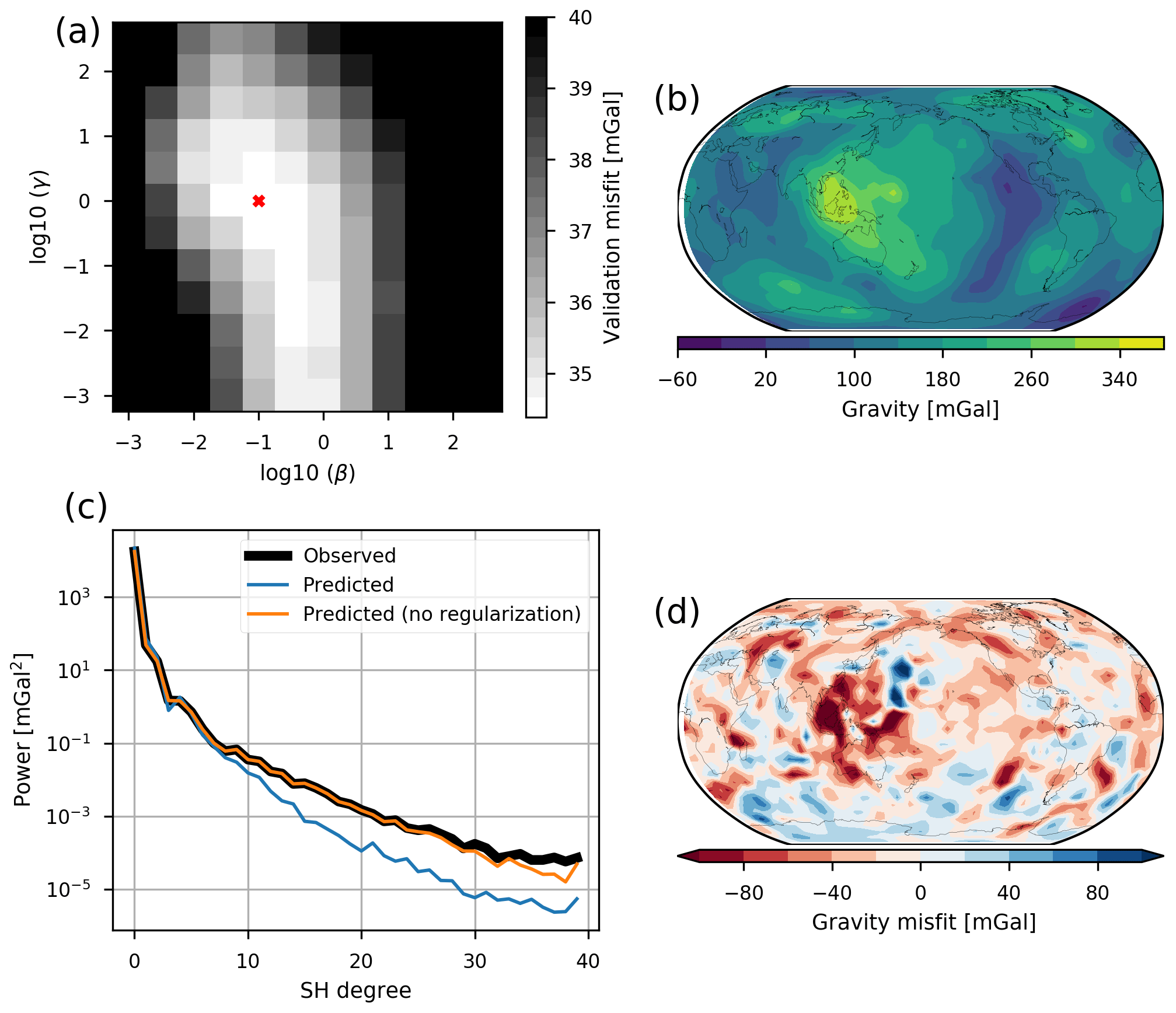
Figure 6Results of the inversion using the crustal residual. (a) Validation misfit as a function of regularization parameter β. (b) Predicted field of the inversion results. (c) Spectral comparison of the input and predicted data. (d) Difference between input and predicted data.
Overall the inverted density variations are much larger for the crustal residual than for the isostatic residual (Fig. 7). In the upper 300 km or so, this is expected, since the lithospheric density structure has not been accounted for by the crustal model. The ocean cooling trend is not imaged well by the vote maps, and as a result, only the Pacific and Indian oceans' spreading ridges are resolved as crude negative density anomalies (Fig. 7a). Some cratons (North America, Eurasia) show strong positive density anomalies (30 kg m−3), but this neither is consistent vertically nor applies to most geographical regions (Fig. 7a and b). Thus, the ability to resolve mantle lithospheric sources is limited and probably contributes to the poor fit of the data.
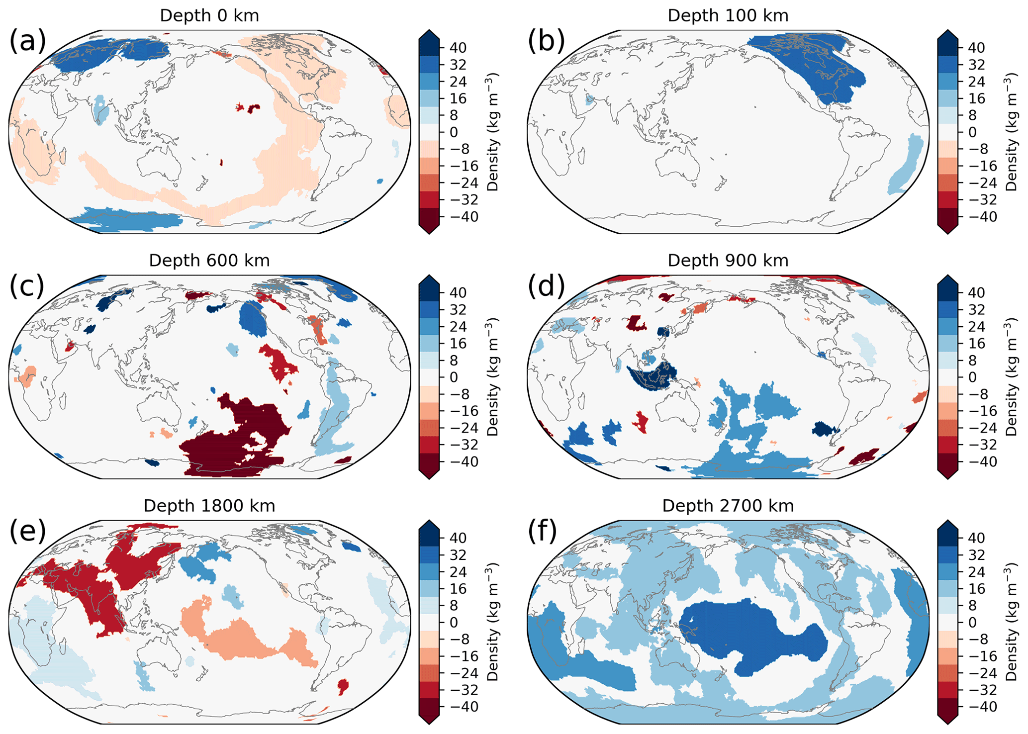
Figure 7Density anomaly slices through selected depths of the inversion results using the crustal residual.
At depths of 600 and 900 km, some subduction-related density anomalies can be seen, but overall correlation is poor. Only in the lowest mantle a more consistent picture emerges, in particular the LLVPs are resolved as positive density anomalies (+40 kg m−3). As in the case with isostatic residual, the African LLVP appears to extend further upwards as a positive density anomaly than the Pacific LLVP (Fig. 7e and f).
4.1 Resolved mantle structure
While the main features observed are the LLVPs, it is important to also scrutinize the results for the remaining mantle. A long-wavelength error in the upper-mantle density structures leads to an incorrect estimate of the density of the LLVPs. In the upper mantle above the transition zone (410–670 km depth) much of the seismic image can be linked to tectonic features: thick and cold lithospheric roots underlie the cratonic cores of the continents and can extend up to 300 km deep (Schaeffer and Lebedev, 2015); the oceans are characterized by a velocity trend related to cooling of the lithosphere (Priestley and McKenzie, 2006); and slabs formed during subduction sink through the mantle, sometimes stagnating at various depths and sometimes passing through the transition zone to the lowermost mantle (e.g. van der Meer et al., 2018).
The cratonic lithospheric mantle density is the result of a complex interaction between temperature, composition and mineralogy (Griffin et al., 2009; Fullea et al., 2009; Afonso et al., 2013). The density increase due to low temperature is probably (partially) offset by its depleted composition (the isopycnic hypothesis; Jordan, 1978). Indeed, a slightly positive density anomaly (+5 to 7.5 kg m−3) is recovered by the inversion with crustal residual in the cratonic cores of North America, central Europe, Siberia and East Antarctica. In contrast, the inversion with the isostatic residual does not show the cratons. The cratonic mantle keels affect surface topography and, hence, are removed by the isostatic correction.
The density of the oceanic mantle is expected to increase with age, following the cooling trend, which also explains seafloor subsidence. The inversion with crustal residual shows some decreased density associated with mid-oceanic ridges, but vote maps are unsuited to resolve the continuous gradient associated with the cooling of the plate. When using the isostatic residual, ocean floor subsidence and the cooling trend has already been accounted for during the isostatic correction and is thus not resolved by the inversion.
Subducted slabs are denser than surrounding mantle immediately after subduction. As the plate sinks, heat diffuses into the plate from the surrounding mantle, so that the plate slowly loses its negative buoyancy. How quickly a subducted plate thermally equilibrates depends on how effectively heat is transported to the slab by convection and conduction. Since some slabs seem to stagnate on mantle discontinuities, it is conceivable for a slab to loose all or most of its negative buoyancy. We compared our results with the slab depth contours from Slab 1.0 (Hayes et al., 2012).
Out of the 12 slabs contained in Slab1.0, only five are detected as positive velocity anomalies based on the vote maps (Fig. 8a) and only at depths greater than 200 km or more. These are Izu–Bonin, Kermadec–Tonga, Kamchatka–Kurils–Japan, South America and Sumatra, according to the terminology of Slab1.0.
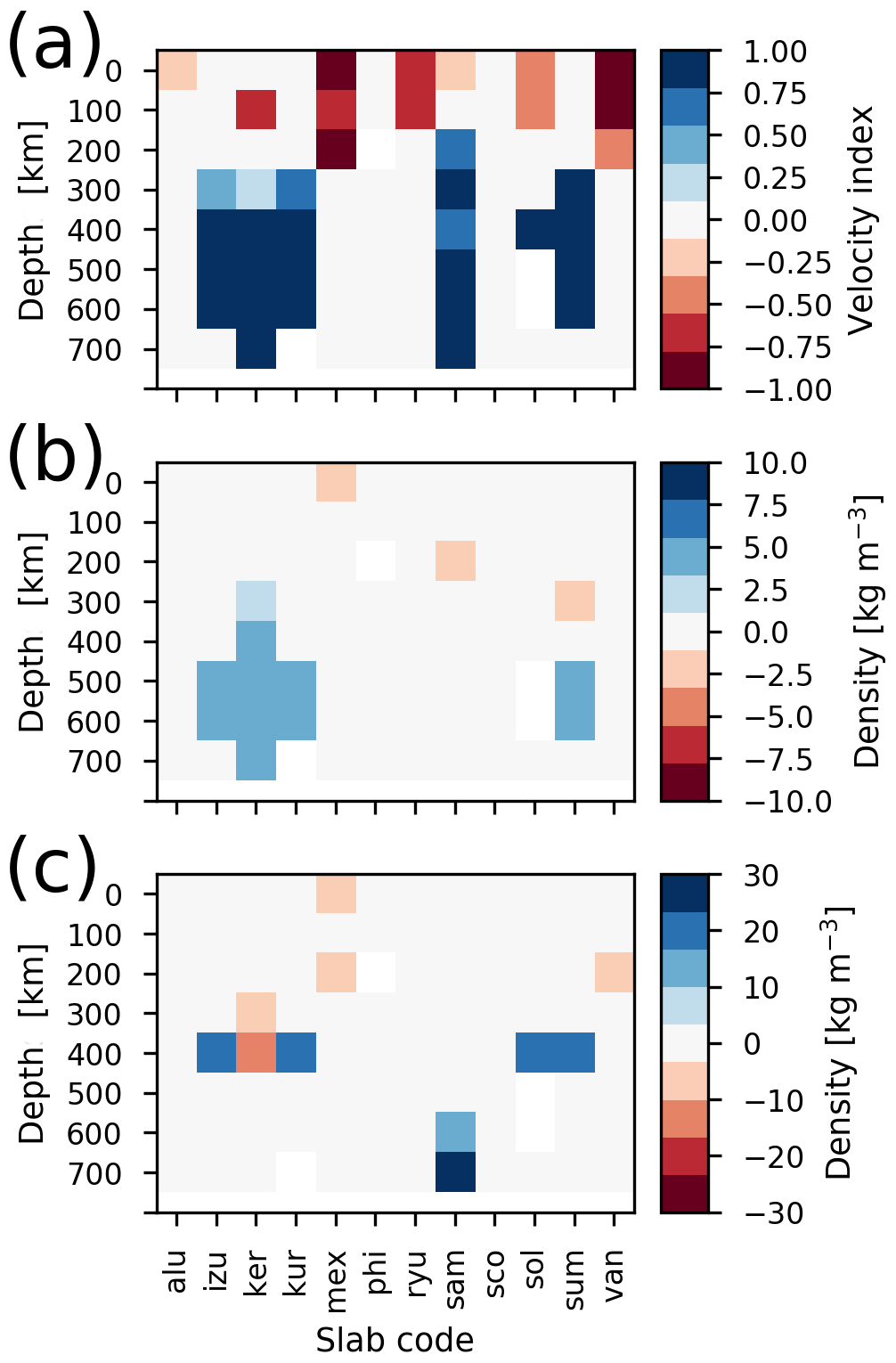
Figure 8Comparison with Slab1.0 (Hayes et al., 2012). The slab codes stand for the following: alu – Alaska–Aleutians; izu – Izu–Bonin; ker – Kermadec–Tonga; kur – Kamchatka–Kurils–Japan; mex – Central America; phi – Philippines; ryu – Ryukyu; sam – South America; sco – Scotia (South Sandwich); sol – Solomon Islands; sum – Sumatra; van – Santa Cruz Islands–Vanuatu–Loyalty Islands. (a) Average value of the velocity anomalies inside the Slab1.0 contour, where 1 = positive, −1 = negative anomaly. (b) Average density anomaly from inversion using the isostatic residual. (c) Average density anomaly from inversion of the crustal residual.
The reason might be that the tomography models are too heterogeneous in quality and resolution to resolve these relatively narrow features. Of course, vote maps are not the only way to extract features from seismic tomographies, and an alternative would be to use the “best” seismic tomography model available instead of a collection of models. But there are no clear criteria to decide which tomography result is the best, except that newer results are probably based on more and better data. Furthermore, there is some evidence that the differences between tomographic models partly reflect different regularization parameters, rather than different resolved features (Root et al., 2016; Root, 2020). Thus, vote maps only extract the features that are resolved by a majority of tomographic models
Still, out of the five detected slabs, four have positive density contrasts (+5 to +10 kg m−3) in the inversion with the isostatic residual (Fig. 8b). However, these density anomalies are not continuous over the entire depth range of the slabs and are limited to depths between 400 and 700 km. Similar results are obtained using the crustal residual as input, but the density anomalies are more sporadic and concentrated at a single depth of 400 km with stronger density variations of up to +30 kg m−3 (Fig. 8c).
Based on these results, we think that our density inversion gives acceptable results overall for most of the mantle. The binary classification scheme we use to extract regions from the vote maps leads to a very rough representation in the upper 300 km, which likely contributes to the poor data fit obtained using the crustal residual. In addition, we assume a constant density contrast over the vertical resolution of 100 km. Thus, the volume of relatively thin structures like slabs might be smeared out over a too large depth range.
4.2 Velocity–density relation
We compare the recovered density values with velocity values from the SMEAN2 tomography, an update of SMEAN (Becker and Boschi, 2002). SMEAN2 is itself an average of three tomography models and agrees reasonably well with the patterns of the vote maps. To correlate velocity and density, every potential density anomaly is assigned the average value of SMEAN2 over the area of the potential density anomaly.
Next, we calculated the distribution of the ρ∕vs ratio at each depth. For this distribution, we used the variability in each density value that we calculated during the cross-validation procedure. In addition, we weighted the distribution by the area of each potential density anomaly. Two histograms were estimated for the fast and slow anomalies.
In the case of the isostatic residual, the median conversion factor changes significantly with depth (Fig. 9a). In the upper 300 km it is on average close to zero, starts to increase at depths greater than 300 km and reaches a maximum of ∼0.2 at 1000 km depth. Remarkably, the conversion factor then decreases rapidly with depth, becoming negative at around 1200 km depth. The distributions at the different depths are highly variable as well. At most depths, the scaling factor shows a multimodal distribution, so there is no single consistent velocity–density relation.
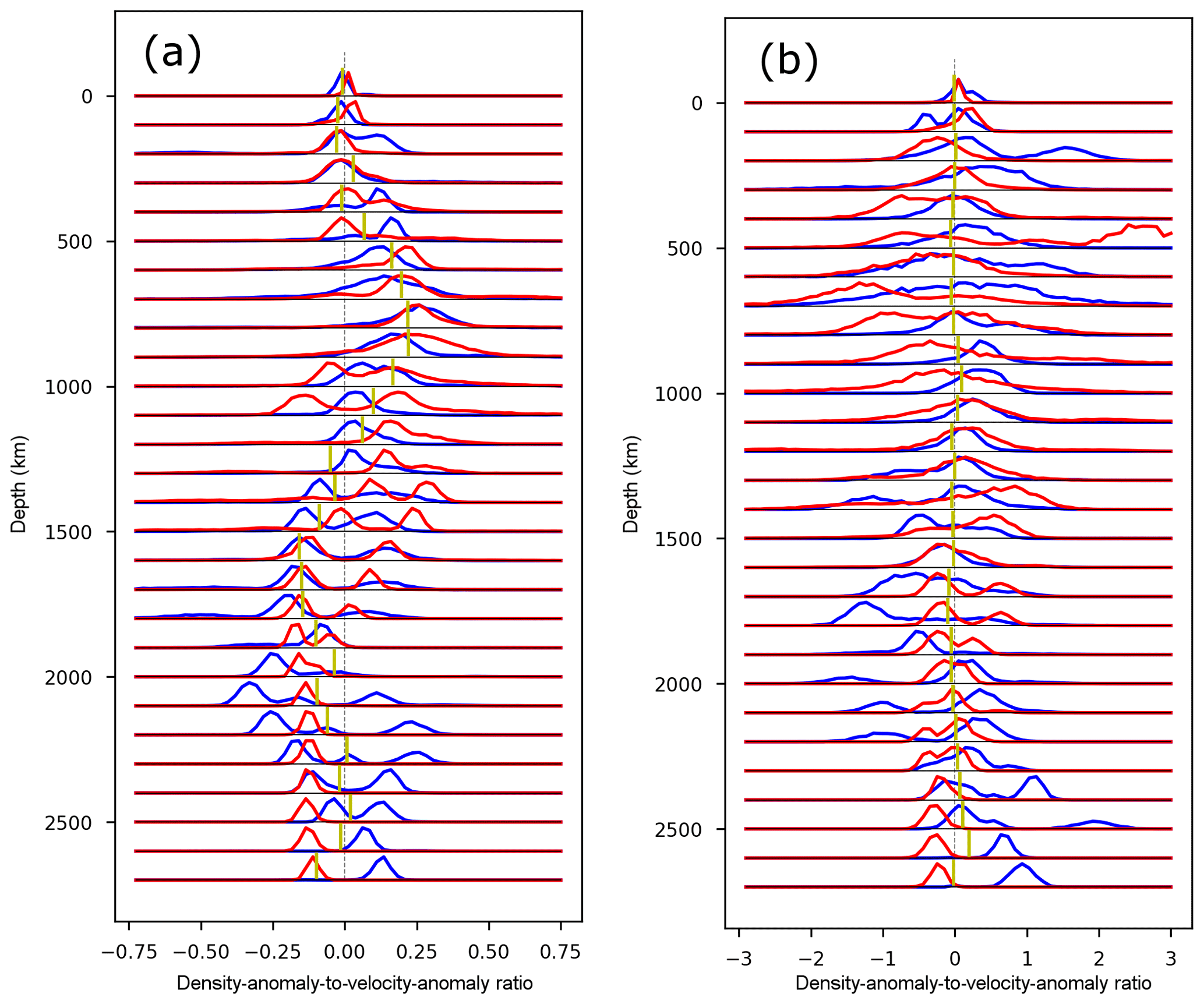
Figure 9Distribution of density-anomaly-to-velocity-anomaly ratios as a function of depth. The blue line is the distribution for fast velocity anomalies, and the red line is for slow velocity anomalies. The yellow line gives the median of the ratio distribution. Note that the median sometimes appears to lie outside the distribution, which is due to heavy tails that are not visible on this scale. Furthermore, the histograms for slow and fast anomalies are scaled to have the same maximum height for easier visual comparison. (a) Scaling for results with isostatic residual. (b) Scaling for results with crustal residuals.
The velocity–density scaling relations we calculated could have the following causes. The small scaling values in the upper 300 km is due to the fact that we use the isostatic residual. The increased scaling factors in the transition zone depths could be related to undulations in the phase transitions depths, because the higher-pressure phases have both higher density and velocity. Thus, any undulation of the phase transition would strongly affect both density and velocity. The negative velocity-anomaly-to-density-anomaly ratios we calculated below 1200 km depth zone can only be explained by compositional variations. In Appendix A we calculate sensitivities of density and velocity to temperature, iron content and MORB (mid-oceanic ridge basalt) fraction changes. We find that the sensitivities to iron content and MORB fraction are fairly constant below the transition zone, whereas the temperature sensitivity slowly decreases with depth. Thus, the velocity and density values below the transition zone could be more indicative of compositional variations than above the transition zone.
The joint geodynamic–tomographic model Gypsum (Simmons et al., 2009) also recovered a depth-variable velocity anomaly to density anomaly scaling of similar magnitude as our results. In addition, they also obtained an increase towards a maximum at around 1000 km depth. However, while their results show a decrease below 1000 km, they did not obtain systematically negative scaling factors, because they regularized towards a thermal scaling factor, which is always positive.
However, the negative conversion factors might also be affected by unmodelled dynamic effects. Depending on the viscosity model, the geoid kernel can become negative at the longest wavelengths in the lower mantle (Steinberger, 2016). This is mainly due to the effect of dynamic topography at the surface and the CMB, which has the opposite sign of the density anomaly causing it. However, we do not think that this effect alone is sufficient to explain the sign change in the lower mantle. We use the gravity field, not the geoid, and the former is more sensitive to the dynamic surface topography, which is predicted to be small, based on our density model (see next section). Still, dynamic compensation of masses in the lower mantle on the CMB could bias our results in the direction of negative conversion factors (see also Sect. 4.4).
In the case of the crustal residual, the increased overall density variation leads to higher velocity anomaly to density anomaly scaling values (Fig. 9b). However, the distribution of the scaling values are so broad that there is not a clear change in the scaling with depth.
4.3 Surface topography
We calculated the contribution of the mantle to surface topography. This allows one to assess the quality of our results, because the predicted mantle topography contribution should be zero for the isostatic residual and equal to the residual topography in the crustal residual case.
In the isostatic case, the upper mantle contributes less than 250 m to surface topography (Fig. 10a). Contrary to expectation, there is a slight positive topographic contribution in some regions with thick lithosphere (North America, eastern Australia, East Antarctica) due to negative density anomalies in the upper mantle. The likely explanation is that we only use the Moho depth to compensate topography, but in reality there is an additional contribution from the lithospheric mantle. Thus, our isostatic Moho depths is too shallow, making the isostatic correction too positive, which is then corrected by the density inversion.
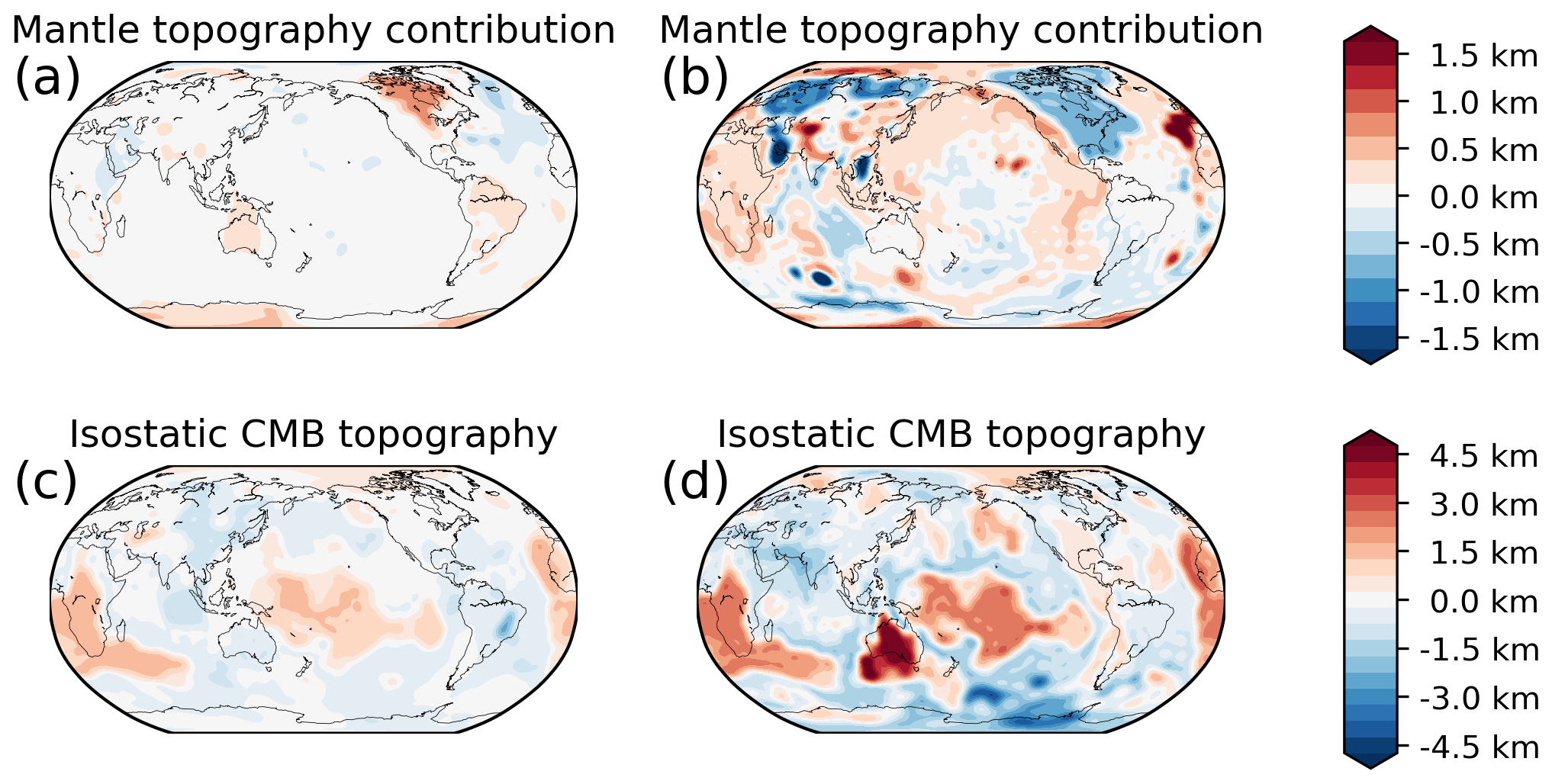
Figure 10Isostatic contributions to boundary deformations from inverted density model. To facilitate comparison with the dynamic topography in Fig. 11 the results have been filtered to spherical harmonic degree 30. (a) Contribution of upper 300 km to surface topography for the inversion results based on the isostatic residual. (b) The same for the results based on the crustal residual. (c) Contribution of the lower 800 km of the mantle to topography at the core–mantle boundary based on the isostatic residual inversion. Positive values indicate a depression of the CMB. (d) The same for the crustal residual inversion.
These results are also confirmed by the dynamic topography calculation. With the two-layer viscosity model that we chose, the topography kernels are essentially zero except for the upper 300 km of the mantle. Hence, the predicted dynamic topography is very similar to the isostatic topography. Even at degree 2, where one would expect the strongest signal from dynamic topography, according to the kernels, there is hardly any topographic contribution, because the high-density LLVPs (the dominating degree 2 structure) are overlaid by negative density anomalies. The existence of a low-density layer on top of the LLVPs was also observed in a mantle convection simulation (Liu and Zhong, 2015).
The inversion results with the crustal residual reproduce the main feature of the residual topography of our crustal model to first order. The isostatic topography contribution of the upper 300 km is considerable (up to 1.5 km). In the North American and Siberian craton, the isostatic topography is mainly negative due to the strong influence of thick, dense lithosphere, but in other areas (e.g. South Africa) the topographic contribution is negative. In the oceans, the expected signal from ocean floor spreading can only be seen in the Pacific. This is because the vote maps only reflect the oceanic cooling trends in a very crude way, such that only the broad ridges in the Pacific can be captured using this technique.
Still, there is qualitative agreement between the residual topography of the crustal model we used and the topography contribution from the upper mantle. The remaining misfit is due to an imperfect crustal model and the poor representation of the lithospheric mantle in the vote maps. In a recent model (Afonso et al., 2019), it was found that topography and the gravity field can be explained by the crust and upper mantle (for wavelengths shorter than spherical harmonic degree 15), while still staying within the uncertainty in the global seismological model Litho1.0 (Pasyanos et al., 2014). This suggests that when using a crustal model to account for the upper Earth, one should jointly consider the uncertainties in the crustal model, possibly even co-inverting a crustal model.
4.4 Impact of CMB topography
We did not explicitly include the gravity effect of CMB deformation in our inversion. To estimate the impact of CMB topography, we use the results based on the isostatic residual gravity. If the lower 800 km of the mantle is isostatically balanced on the CMB and assuming a density contrast of 4500 kg m−3 at the CMB, the inverted density structure would lead to CMB undulations of ±1200 m. The CMB topography is dominated by the depressions underneath Africa and the Pacific that are caused by the increased density of the LLVPs. At satellite altitude, these undulations would cause a gravity response of ±20 mGal. Due to the great depth of the source, the gravity response is anti-correlated with the proper gravity effect of the density anomalies in the lower 800 km of the mantle. Thus, the gravity effect of isostatic CMB deformations would reduce the gravity effect associated with lower-mantle density anomalies from ±30 to ±15 mGal but does not affect the spatial pattern. Hence, the actual density anomalies in the lower mantle would have to be twice as large to produce the same gravity effect as without CMB deformation. Therefore, we expect that the inversion underestimates the true density variations in the lowermost mantle.
These results also hold if dynamic topography is calculated using a two-layer viscosity model at least at the wavelengths where the gravity signal of the CMB would be visible (compare Figs. 10d and 11d). However, several studies have found that the convection dynamics in the lowest mantle might be more complicated. Viscosity probably varies laterally, because of strong temperature or composition differences (Lassak et al., 2010; Deschamps et al., 2018). In addition, post-perovskite might have much lower viscosity than perovskite (Deschamps and Li, 2019). In some scenarios the CMB deformation decorrelates from the density distribution in the lowest mantle. These findings imply that there is an additional source of uncertainty for the LLVP densities that we estimated.
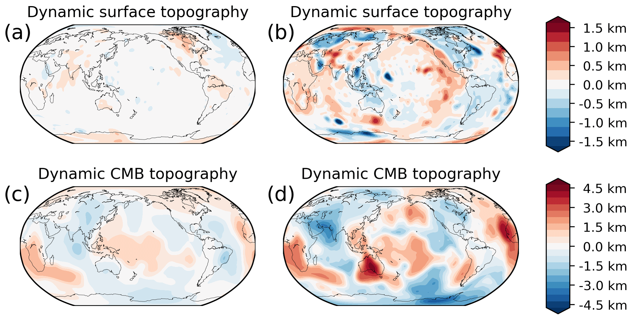
Figure 11Dynamic contributions to boundary deformations from inverted density model and a two-layer viscosity model. The results are filtered to spherical harmonic degree 30. (a) Contribution of upper 300 km to surface topography for the inversion results based on the isostatic residual. (b) The same for the results based on the crustal residual. Note that some structures appear which were not seen in Fig. 10b. This is caused by strong density anomalies below 300 km depth, which were not considered in the isostatic calculation shown in Fig. 10b. (c) Dynamic core–mantle boundary topography based on the isostatic residual inversion. Positive values indicate a depression of the CMB. (d) The same for the crustal residual inversion.
Comparing our results with published CMB topography estimates based on seismological methods (Morelli and Dziewonski, 1987; Doornbos and Hilton, 1989; Sze and van der Hilst, 2003; Tanaka, 2010), we find that none of the models contain the first-order pattern of CMB depressions beneath Africa and the central Pacific, seen in our maps (Fig. 10c, d). In terms of the magnitude, the CMB topography based on the isostatic residual are much smaller than any seismic determination except Sze and van der Hilst (2003), whereas the crustal residual CMB topography has similar range as Doornbos and Hilton (1989) and Morelli and Dziewonski (1987).
4.5 Isostatic residual vs. crustal correction
The results obtained with isostatic and crustal residual disagree substantially. The correlation coefficient calculated for individual depth slices is typically less than 0.5 and even negative for some depths. The highest correlations are found in the depth ranges of 2500–2800 and 1500–2000 km and are mainly due to the influence of the LLVPs. In addition, the magnitude of the density anomalies is on average 4 times larger based on the crustal residual, which agrees with the relative magnitude of the input gravity fields.
Based on the fit to the data, the isostatic residual is preferred, because it achieves both higher absolute and relative data fit. However, the isostatic Moho depths disagree with the seismological determinations. Furthermore, the crustal residual lacks a correction for the oceanic cooling trend, which clearly contributes to the crustal residual. Thus, the better data fit preference for the isostatic residual is not as straightforward.
In any case, the isostatic and crustal residuals are extreme examples of how the crust and upper mantle can be accounted for in a gravity inversion. Our results clearly demonstrate that these different approaches lead to an enormous spread in terms of the recovered densities in the mantle. At the same time, signals from the deep Earth in terms of gravity or topography might affect modelling of the upper Earth. Commonly, high-pass filtering is used to remove the signal of the deep Earth (Bowin, 1991), but this is clearly insufficient, due to the spectral overlap (Root et al., 2015). Thus, a coupled approach that simultaneously considers the entire crust and mantle is required in order to properly model the gravity field and Earth's topography.
4.6 Implications for LLVP temperature and composition
Broadly speaking, the LLVPs could originate from any combination of increased temperature and compositional variation. After their first discovery, the LLVP were initially considered as a purely thermal feature: two “superplumes” that rise from the core–mantle boundary (Dziewonski, 1984). However, even if the LLVPs are purely due to temperature increase, a more likely explanation is that they are swarms of smaller plumes that are smeared due to the limited resolution of seismic tomographies (Schubert et al., 2004; Schuberth et al., 2009), with an additional influence from the stability field of post-perovskite (Koelemeijer et al., 2018).
In contrast to this isochemical view, some authors have proposed that the LLVPs are chemically distinct from the normal (pyrolitic) mantle. The chemical distinctiveness of the LLVP can either be accumulated over time or be a primitive reservoir that separated early in Earth's history (Deschamps et al., 2012). A likely process for accumulation is the separation of oceanic crust from subducted lithosphere (Mulyukova et al., 2015). However, these two hypotheses are not mutually exclusive, and a small amount of subducted oceanic lithosphere might be incorporated in pre-existing structure, as proposed in the basal melange (BAM) hypothesis (Tackley, 2012). If the LLVPs have a compositional component, they have to be intrinsically denser than surrounding pyrolitic mantle to have remained near the core–mantle boundary, despite very high temperatures. If the LLVPs are indeed old features, this would also explain the proposed spatial correlation between plume generation and the edges of the LLVPs over the last 200 million years (Burke et al., 2008).
Our inversion results indicate a positive density anomaly for the LLVPs both using isostatic and crustal residual. This would rule out a purely thermal origin of the LLVPs, since such a scenario would lead to negative density anomalies.
In order to test different scenarios using our inversion results, we make use of the petrological database of Stixrude and Lithgow-Bertelloni (2011). We construct a simple adiabatic model (see Appendix A) based on a pyrolitic composition for the mantle (Stixrude and Lithgow-Bertelloni, 2012) that serves as reference model. The adiabatic model is entirely self-consistent, and the only free parameter is the temperature at the top of the model, which we adjusted in order to fit the surface wave dispersion curves from PREM (Dziewonski and Anderson, 1981). Unlike previous thermochemical interpretations for the lower mantle (e.g. Deschamps et al., 2012), this corrects for the bias between the petrophysical database and PREM. Next, we applied first-order perturbations to the model and obtained sensitivities of shear wave velocity and density to changes in temperature, iron content and fraction of mid-ocean ridge basalt (MORB).
We assume a negative S-wave velocity deviation of 2 % for the LLVPs, since most mantle tomographies display roughly this amount of slowness. Our inversion results would place the density anomaly of the LLVP between 0.1 % (isostatic residual) and 0.3 % (crustal residual), but due to possible isostatic compensation at the CMB, (Sect. 4.4), the density anomalies could be twice as large (up to 0.6 %).
A temperature increase of 670 K leads to the required velocity reduction; however it would also entail a density change of −1 %, which would be incompatible with our findings. Likewise, a 2.6 % increase in iron content (without temperature change) fits the velocity reduction but leads to a density increase of 1.6 %. To fit both velocity and our lowest density estimate, a temperature increase of 380 K and an iron increase of 1.1 % is required, while our highest density estimate would require changes of 260 K and 1.6 % FeO respectively.
Adding a MORB fraction leads to higher required temperatures, because MORB is slightly faster than pyrolitic mantle at the depths of the LLVPs, according to our petrophysical calculations. Our lowest density estimate (+0.1 %) would require a temperature change of +870 K and a MORB fraction of 40 %, and the highest density estimate (+0.6 %) requires +960 K and 58 % MORB. Deschamps et al. (2012) also found high excess temperatures (+1500 K) were necessary to explain the shear wave velocity and bulk sound speed if the LLVPs are MORB-enriched. However, our interpretation is dependent on the petrological database of Stixrude and Lithgow-Bertelloni (2011), which is based on sparse measurements at extremely high pressures. Recent measurements of calcium–perovskite (Ca–Pv) (Gréaux et al., 2019; Thomson et al., 2019) imply that seismic velocities in MORB-enriched zones would be lower than thought previously. Thus, less extreme temperatures would be required to reconcile increased density and reduced velocity. Furthermore, the chemical composition of MORB is highly variable, especially its iron content (Deschamps et al., 2012), which could also strongly affect the impact of mixing a MORB fraction into a pyrolitic mantle.
Based on our results it is difficult to express preference for MORB or iron enrichment. Since MORB is introduced to the mantle by subduction, plate reconstructions place some constraints on the amount of MORB produced. Stixrude and Lithgow-Bertelloni (2012) estimate that the total amount of basalt input into the mantle corresponds to about 10 % of the volume of the mantle. As an absolute upper limit, assuming the LLVPs have a height of 800 km and cover 25 % of the core surface area, the volume would be around 4 % of the total mantle. Thus, to reach a MORB fraction of 60 % in the LLVPs, about a fourth of the total generated subducted basalt would need to accumulate.
In this paper we have presented how the gravity field and tomographic vote maps can be combined to estimate the density distribution inside the mantle. We have shown that the method is able to reasonably recover expected features in the mantle without requiring any information about the viscosity structure. Still, our recovered density structure leads to qualitative agreement between isostatic and residual topography. Furthermore, our results indicate that the LLVPs are slightly denser and hence chemically distinct.
In our first-order analysis, the nonlinear dependencies of velocity and density, the impact of melt, heterogeneity inside the LLVPs, and the possible presence of post-perovskite is neglected. However, our results can be reconciled with our present knowledge about rock properties at these extreme conditions.
One important difference compared to previous methods is that in our method density is free to vary independent of seismic velocity. While this gives the necessary freedom to the density inversion, it ignores the strong evidence for the important role of temperature. In the future, more precise petrophysical data could help to put constraints on the relative importance of temperature and composition. This would also help to reconcile our results with previous viscosity inversions.
Furthermore, our results show that the lithospheric mantle is critical to resolve disagreements between bottom-up and top-down methods. In fact, depending on how the lithosphere is treated, the inverted density anomalies can change by a factor of 4. Thus, a combined approach is necessary, where the uncertainties in seismic determinations of the lithosphere are considered in conjunction with signals resulting from deeper density anomalies.
Our inversion breaks down the mantle volume into discrete volumes with a constant density anomaly. This reduces the number of unknowns compared to a continuous inversion and means that less regularization is required. However, using vote maps to extract features from a collection of seismic tomographies is the most basic way to do this, and a more refined method (e.g. Fadel et al., 2015) could lead to better constrained volumes. In particular it might benefit an inversion if uncertainties could be placed on the size and position of the volumetric features to allow them to change during inversion.
Instead of relying on seismic tomographies or derived quantities like vote maps, it might be beneficial to stay closer to seismic data. The canonical choice would be seismic travel times and normal modes (as in Dziewonski and Anderson, 1981), but there are more uncommon seismic products that might provide additional constraints. For instance, core-diffracted waves are very sensitive to velocity near the CMB (Hosseini and Sigloch, 2015).
We derived a simple 1-D adiabatic model of Earth's mantle, based on a petrological database (Stixrude and Lithgow-Bertelloni, 2005, 2011). We assume a pyrolitic composition (45.1 % SiO2, 38.1 % MgO, 8.0 % FeO, 3.3 % Al2O3, 3.1 % CaO) throughout the entire mantle.
The main relations – density ρ(P,T), specific heat capacity cp(P,T) and heat expansivity α(P,T) – are functions of temperature and pressure and are calculated using the Stixrude database with PerpleX (Connolly, 2009). Pressure is purely hydrostatic as follows:
The temperature is purely adiabatic, such that
The gravity acceleration at a specific depth is determined by the internal mass at that depth
and the internal mass is decreasing with depth according to
This set of equations can be solved by finite differences if the pressure, temperature and gravity strength are specified at the top of the model domain. First, the ρ, cp and α belonging to these P−T conditions are calculated using PerpleX (Connolly, 2009). Then, these values are used to update pressure, temperature and internal mass as follows:
This process is repeated iteratively from the top of the model domain down to the core–mantle boundary, with a step size Δr of 1 km.
We begin this integration at a depth of 80 km, with a pressure of 2.5 GPa and g=9.81 m s−2. In order to determine the temperature at the top, we relied on PREM (Dziewonski and Anderson, 1981). At first we attempted to directly minimize the difference between the velocities in PREM and the modelled velocity from PerpleX. However, this approach was unsuccessful, because the depths of the main discontinuities in PREM (410, 660 km) are incompatible with the Stixrude database.
Instead, we relied on Rayleigh wave dispersion curves to choose the temperature at the top of the model. Using Mineos (Masters et al., 2019) we calculated the phase velocity of the fundamental Rayleigh wave between frequencies of 0 and 50 mHz for PREM and for the adiabatic model, for temperatures at the top between 1300 and 1800 K in steps of 50 K. We found that a top temperature of 1550 K gives the best fit to the PREM dispersion curves (Fig. A1a), if equal weight is given to phase velocities at all periods. In particular, we find that the T=1550 K model fits the dispersion curve data with an average relative accuracy of 0.3 %, which is similar to the fit with which PREM fits the data used in its construction. Thus, our model is equivalent to PREM with respect to the dispersion curve data. During these calculations we also found that the presence of a post-perovskite phase completely prevents fitting the long-period dispersion curves, so we excluded post-perovskite from the PerpleX calculations.
The resulting temperature curve for the preferred model is nearly linear but shows a distinct kink below the 660 km discontinuity, due to the different properties of perovskite and a slower temperature increase at greater depths due to the decrease in thermal expansivity α (Fig. A1b). The temperature at the bottom of the mantle is roughly 2350 K. The pressure curve is also nearly linear but is slightly bent due to the increase in density with depth.
We then applied first-order perturbations in terms of temperature, iron content and mid-oceanic ridge basalt (MORB) fraction to the adiabatic model. The vertical resolution of our density models is 100 km, so we applied the perturbation over the same depth range. To determine the sensitivity to temperature variations, we simply used our existing lookup table from PerpleX, while for compositional variations we determined new phase equilibria and corresponding rock properties with FeO content increased by 1 %. For the MORB we proceeded somewhat differently, because the MORB is likely not in phase equilibrium with the surrounding mantle rocks, due to the long timescale of chemical diffusion (Stixrude and Lithgow-Bertelloni, 2012). Thus, we determined the phase equilibrium of a pure MORB and then calculated velocities and densities as volume averages of the MORB fraction and the surrounding mantle. These results can be used together to determine how sensitive vs and density are to changes in temperature, iron content or MORB fraction (Fig. A2).
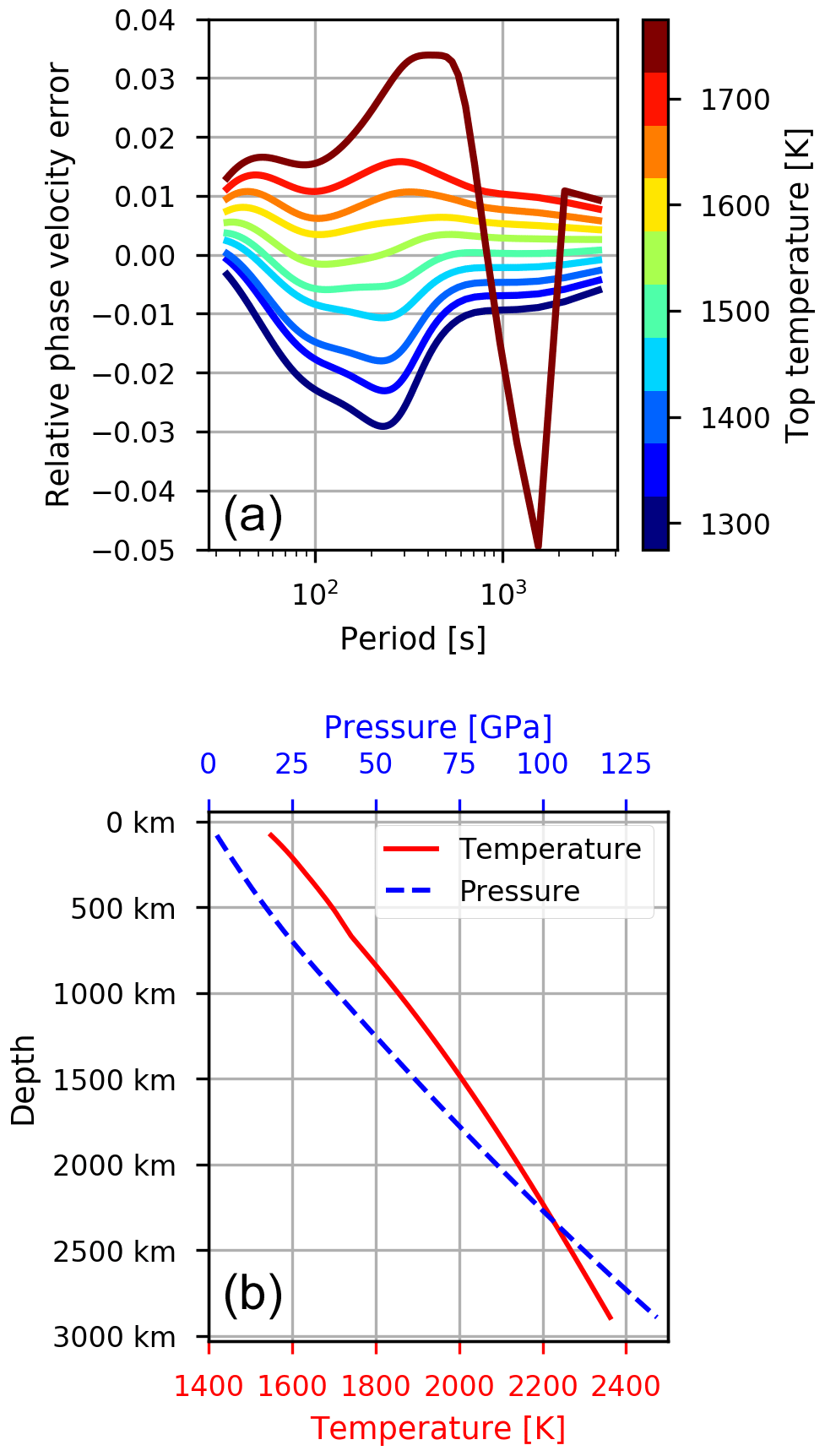
Figure A1Results of the adiabatic model. (a) Rayleigh temperatures at the top of the adiabatic model (80 km). (b) Temperature and pressure profiles for the preferred model with Ttop=1550 K.
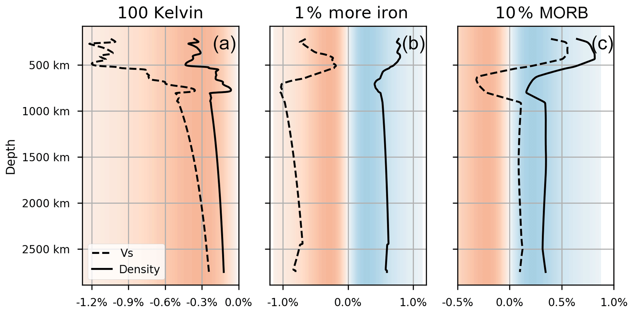
Figure A2First-order perturbation curves for deviations from a adiabatic, hydrostatic model with pyrolitic composition. The red and blue background shading indicates negative and positive changes of the respective quantity. (a) Relative change for a temperature change of 100 K. (b) Relative change for including 1 % more FeO. (c) Relative change for a mixture of 90 % pyrolite and 10 % MORB.
All input data of the study are freely available. Gravity data can be downloaded from International Centre for Global Earth Models (ICGEM); vote maps are available from http://www.earth.ox.ac.uk/~smachine (Hosseini et al., 2018); the crustal model is available in the Supplement of Szwillus et al. (2019). Mineos can be downloaded via the Computational Infrastructure for Geodynamics (http://geodynamics.org/cig/software/mineos, Masters et al., 2019); PerpleX is available from the author's website http://www.perplex.ethz.ch/ (Connolly, 2020).
All software required to repeat the calculations presented here is available on GitHub (https://github.com/wokos/llvp-density, Szwillus, 2020).
The supplement related to this article is available online at: https://doi.org/10.5194/se-11-1551-2020-supplement.
JE developed the initial idea of the project; WS developed the code and ran the calculations. BS benchmarked the topography kernel calculations. WS prepared the article with contributions from JE and BS.
The authors declare that they have no conflict of interest.
The authors thank John Brodholt for his comments on an earlier version of this manuscript. We also thank the two anonymous reviewers for their constructive criticism that helped improve our article.
This work was carried out as part of the European Space Agency's Support to Science Element “3D Earth – A dynamic living planet”. Bernhard Steinberger received partial support from the Centre of Excellence project 223272 through the Research Council of Norway.
This paper was edited by Taras Gerya and reviewed by two anonymous referees.
Afonso, J. C., Fullea, J., Griffin, W. L., Yang, Y., Jones, A. G., D. Connolly, J. A., and O'Reilly, S. Y.: 3-D multiobservable probabilistic inversion for the compositional and thermal structure of the lithosphere and upper mantle. I: A priori petrological information and geophysical observables, J. Geophys. Res.-Sol. Ea., 118, 2586–2617, https://doi.org/10.1002/jgrb.50124, 2013. a
Afonso, J. C., Salajegheh, F., Szwillus, W., Ebbing, J., and Gaina, C.: A global reference model of the lithosphere and upper mantle from joint inversion and analysis of multiple data sets, Geophys. J. Int., 217, 1602–1628, https://doi.org/10.1093/gji/ggz094, 2019. a
Amante, C. and Eakins, B. W.: ETOPO1 Global Relief Model converted to PanMap layer format, NOAA-National Geophysical Data Center, PANGAEA https://doi.org/10.1594/PANGAEA.769615, 2009. a
Ballmer, M. D., Schmerr, N. C., Nakagawa, T., and Ritsema, J.: Compositional mantle layering revealed by slab stagnation at ∼1000-km depth, Science Advances, 1, e1500815, https://doi.org/10.1126/sciadv.1500815, 2015. a
Ballmer, M. D., Houser, C., Hernlund, J. W., Wentzcovitch, R. M., and Hirose, K.: Persistence of strong silica-enriched domains in the Earth's lower mantle, Nat. Geosci., 10, 236–240, https://doi.org/10.1038/NGEO2898, 2017. a
Becker, T. W. and Boschi, L.: A comparison of tomographic and geodynamic mantle models, Geochem. Geophy. Geosy., 3, 2001GC000168, https://doi.org/10.1029/2001GC000168, 2002. a
Bouman, J., Ebbing, J., Meekes, S., Fattah, R. A., Fuchs, M., Gradmann, S., Haagmans, R., Lieb, V., Schmidt, M., Dettmering, D., and Bosch, W.: GOCE gravity gradient data for lithospheric modeling, Int. J. Appl. Earth Obs., 35, 16–30, https://doi.org/10.1016/j.jag.2013.11.001, 2013. a
Bowin, C.: The Earth's gravity field and plate tectonics, Tectonophysics, 187, 69–89, 1991. a
Burke, K., Steinberger, B., Torsvik, T. H., and Smethurst, M. A.: Plume Generation Zones at the margins of Large Low Shear Velocity Provinces on the core–mantle boundary, Earth Planet. Sc. Lett., 265, 49–60, https://doi.org/10.1016/j.epsl.2007.09.042, 2008. a, b
Chilès, J.-P. and Delfiner, P.: Geostatistics: Modeling spatial uncertainty, 2nd Edn., Wiley series in probability and statistics, vol. 713, Wiley, Hoboken, NJ, https://doi.org/10.1002/9781118136188, 2012. a
Connolly, J. A. D.: The geodynamic equation of state: What and how, Geochem. Geophy. Geosy., 10, Q10014, https://doi.org/10.1029/2009GC002540, 2009. a, b
Connolly, J. A. D.: PerpleX, available at: http://www.perplex.ethz.ch/, last access: 18 August 2020. a
Conrad, C. P., Steinberger, B., and Torsvik, T. H.: Stability of active mantle upwelling revealed by net characteristics of plate tectonics, Nature, 498, 479–482, https://doi.org/10.1038/nature12203, 2013. a
Deschamps, F. and Li, Y.: Core–Mantle Boundary Dynamic Topography: Influence of Postperovskite Viscosity, J. Geophys. Res.-Sol. Ea., 124, 9247–9264, https://doi.org/10.1029/2019JB017859, 2019. a, b
Deschamps, F., Cobden, L., and Tackley, P. J.: The primitive nature of large low shear-wave velocity provinces, Earth Planet. Sc. Lett., 349–350, 198–208, https://doi.org/10.1016/j.epsl.2012.07.012, 2012. a, b, c, d, e, f
Deschamps, F., Rogister, Y., and Tackley, P. J.: Constraints on core–mantle boundary topography from models of thermal and thermochemical convection, Geophys. J. Int., 212, 164–188, https://doi.org/10.1093/gji/ggx402, 2018. a, b
Doornbos, D. J. and Hilton, T.: Models of the core-mantle boundary and the travel times of internally reflected core phases, J. Geophys. Res.-Sol. Ea., 94, 15741–15751, https://doi.org/10.1029/JB094iB11p15741, 1989. a
Dziewonski, A. M.: Mapping the lower mantle: Determination of lateral heterogeneity in P velocity up to degree and order 6, J. Geophys. Res.-Sol. Ea., 89, 5929–5952, https://doi.org/10.1029/JB089iB07p05929, 1984. a
Dziewonski, A. M. and Anderson, D. L.: Preliminary reference Earth model, Phys. Earth Planet. In., 25, 297–356, https://doi.org/10.1016/0031-9201(81)90046-7, 1981. a, b, c
Efron, B. and Gong, G.: A leisurely look at the bootstrap, the jackknife, and cross-validation, Am. Stat., 37, 36–48, 1983. a
Fadel, I., van der Meijde, M., Kerle, N., and Lauritsen, N.: 3D object-oriented image analysis in 3D geophysical modelling: Analysing the central part of the East African Rift System, Int. J. Appl. Earth Obs., 35, 44–53, https://doi.org/10.1016/j.jag.2013.11.004, 2015. a
Farquharson, C. G. and Oldenburg, D. W.: A comparison of automatic techniques for estimating the regularization parameter in non-linear inverse problems, Geophys. J. Int., 156, 411–425, https://doi.org/10.1111/j.1365-246X.2004.02190.x, 2004. a
Flament, N., Gurnis, M., and Müller, R. D.: A review of observations and models of dynamic topography, Lithosphere-US, 5, 189–210, 2013. a
Fullea, J., Afonso, J. C., Connolly, J. A. D., Fernàndez, M., García-Castellanos, D., and Zeyen, H.: LitMod3D: An interactive 3-D software to model the thermal, compositional, density, seismological, and rheological structure of the lithosphere and sublithospheric upper mantle, Geochem. Geophy. Geosy., 10, Q08019, https://doi.org/10.1029/2009GC002391, 2009. a
Garnero, E. J., McNamara, A. K., and Shim, S.-H.: Continent-sized anomalous zones with low seismic velocity at the base of Earth's mantle, Nat. Geosci., 9, 481–489, https://doi.org/10.1038/ngeo2733, 2016. a, b
Gréaux, S., Irifune, T., Higo, Y., Tange, Y., Arimoto, T., Liu, Z., and Yamada, A.: Sound velocity of CaSiO3 perovskite suggests the presence of basaltic crust in the Earth's lower mantle, Nature, 565, 218–221, https://doi.org/10.1038/s41586-018-0816-5, 2019. a
Griffin, W. L., O'Reilly, S. Y., Afonso, J. C., and Begg, G. C.: The Composition and Evolution of Lithospheric Mantle: A Re-evaluation and its Tectonic Implications, J. Petrol., 50, 1185–1204, https://doi.org/10.1093/petrology/egn033, 2009. a, b
Hager, B. H. and O'Connell, R. J.: Kinematic models of large-scale flow in the Earth's mantle, J. Geophys. Res.-Sol. Ea., 84, 1031–1048, https://doi.org/10.1029/JB084iB03p01031, 1979. a, b, c, d
Hager, B. H., Clayton, R. W., Richards, M. A., Comer, R. P., and Dziewonski, A. M.: Lower mantle heterogeneity, dynamic topography and the geoid, Nature, 313, 541–545, https://doi.org/10.1038/313541a0, 1985. a
Hayes, G. P., Wald, D. J., and Johnson, R. L.: Slab1.0: A three-dimensional model of global subduction zone geometries, J. Geophys. Res.-Sol. Ea., 117, B01302, https://doi.org/10.1029/2011JB008524, 2012. a, b
Hosseini, K. and Sigloch, K.: Multifrequency measurements of core-diffracted P waves (Pdiff) for global waveform tomography, Geophys. J. Int., 203, 506–521, https://doi.org/10.1093/gji/ggv298, 2015. a
Hosseini, K., Matthews, K. J., Sigloch, K., Shephard, G. E., Domeier, M., and Tsekhmistrenko, M.: SubMachine: Web-Based Tools for Exploring Seismic Tomography and Other Models of Earth's Deep Interior, Geochem. Geophy. Geosy., 19, 1464–1483, https://doi.org/10.1029/2018GC007431, 2018 (data available at: http://www.earth.ox.ac.uk/~smachine, last access: 18 August 2020). a, b
Ishii, M. and Tromp, J.: Normal-mode and free-Air gravity constraints on lateral variations in velocity and density of Earth's mantle, Science, 285, 1231–1236, https://doi.org/10.1126/science.285.5431.1231, 1999. a
Jordan, T. H.: Composition and development of the continental tectosphere, Nature, 274, 544–548, https://doi.org/10.1038/274544a0, 1978. a
Karato, S.-i.: Importance of anelasticity in the interpretation of seismic tomography, Geophys. Res. Lett., 20, 1623–1626, https://doi.org/10.1029/93GL01767, 1993. a
King, S. D.: The viscosity structure of the mantle, Rev. Geophys., 33, 11–17, https://doi.org/10.1029/95RG00279, 1995. a
King, S. D.: An evolving view of transition zone and midmantle viscosity, Geochem. Geophy. Geosy., 17, 1234–1237, https://doi.org/10.1002/2016GC006279, 2016. a
King, S. D. and Masters, G.: An inversion for radial viscosity structure using seismic tomography, Geophys. Res. Lett., 19, 1551–1554, https://doi.org/10.1029/92GL01700, 1992. a
Koelemeijer, P., Deuss, A., and Ritsema, J.: Density structure of Earth's lowermost mantle from Stoneley mode splitting observations, Nature Commun., 8, 15241, https://doi.org/10.1038/ncomms15241, 2017. a, b
Koelemeijer, P., Schuberth, B., Davies, D. R., Deuss, A., and Ritsema, J.: Constraints on the presence of post-perovskite in Earth's lowermost mantle from tomographic-geodynamic model comparisons, Earth Planet. Sc. Lett., 494, 226–238, https://doi.org/10.1016/j.epsl.2018.04.056, 2018. a
Laske, G., Masters, T. G., Ma, Z., and Pasyanos, M. E.: Update on CRUST1.0 - A 1-degree Global Model of Earth's Crust, Geophys. Res. Abstr., EGU2013-2658, EGU General Assembly 2013, Vienna, Austria, available at: https://igppweb.ucsd.edu/~gabi/crust1.html (last access: 18 August 2020), 2013. a
Lassak, T. M., McNamara, A. K., Garnero, E. J., and Zhong, S.: Core–mantle boundary topography as a possible constraint on lower mantle chemistry and dynamics, Earth Planet. Sc. Lett., 289, 232–241, https://doi.org/10.1016/j.epsl.2009.11.012, 2010. a
Lau, H. C. P., Mitrovica, J. X., Davis, J. L., Tromp, J., Yang, H.-Y., and Al-Attar, D.: Tidal tomography constrains Earth's deep-mantle buoyancy, Nature, 551, 321–326, https://doi.org/10.1038/nature24452, 2017. a
Lekic, V., Cottaar, S., Dziewonski, A., and Romanowicz, B.: Cluster analysis of global lower mantle tomography: A new class of structure and implications for chemical heterogeneity, Earth Planet. Sc. Lett., 357–358, 68–77, https://doi.org/10.1016/j.epsl.2012.09.014, 2012. a, b
Liu, X. and Zhong, S.: The long-wavelength geoid from three-dimensional spherical models of thermal and thermochemical mantle convection, J. Geophys. Res.-Sol. Ea., 120, 4572–4596, https://doi.org/10.1002/2015JB012016, 2015. a
Masters, G., Woodhouse, J. H., and Freeman, G.: Mineos, available at: https://geodynamics.org/cig/software/mineos/ (last access: 18 August 2020), 2019. a, b
Molnar, P., England, P. C., and Jones, C. H.: Mantle dynamics, isostasy, and the support of high terrain, J. Geophys. Res.-Sol. Ea., 120, 1932–1957, https://doi.org/10.1002/2014jb011724, 2015. a, b
Morelli, A. and Dziewonski, A. M.: Topography of the core–mantle boundary and lateral homogeneity of the liquid core, Nature, 325, 678–683, https://doi.org/10.1038/325678a0, 1987. a
Moulik, P. and Ekström, G.: The relationships between large-scale variations in shear velocity, density, and compressional velocity in the Earth's mantle, J. Geophys. Res.-Sol. Ea., 121, 2737–2771, https://doi.org/10.1002/2015JB012679, 2016. a
Mulyukova, E., Steinberger, B., Dabrowski, M., and Sobolev, S. V.: Survival of LLSVPs for billions of years in a vigorously convecting mantle: Replenishment and destruction of chemical anomaly, J. Geophys. Res.-Sol. Ea., 120, 3824–3847, https://doi.org/10.1002/2014JB011688, 2015. a, b
Pail, R., Goiginger, H., Schuh, W.-D., Höck, E., Brockmann, J. M., Fecher, T., Gruber, T., Mayer-Gürr, T., Kusche, J., Jäggi, A., and Rieser, D.: Combined satellite gravity field model GOCO01S derived from GOCE and GRACE, Geophys. Res. Lett., 37, L20314, https://doi.org/10.1029/2010GL044906, 2010. a
Pasyanos, M. E., Masters, T. G., Laske, G., and Ma, Z.: LITHO1.0: An updated crust and lithospheric model of the Earth, J. Geophys. Res.-Sol. Ea., 119, 2153–2173, https://doi.org/10.1002/2013jb010626, 2014. a, b
Priestley, K. and McKenzie, D.: The thermal structure of the lithosphere from shear wave velocities, Earth Planet. Sc. Lett., 244, 285–301, https://doi.org/10.1016/j.epsl.2006.01.008, 2006. a
Ricard, Y., Richards, M., Lithgow-Bertelloni, C., and Le Stunff, Y.: A geodynamic model of mantle density heterogeneity, J. Geophys. Res.-Sol. Ea., 98, 21895–21909, https://doi.org/10.1029/93JB02216, 1993. a
Richards, M. A. and Hager, B. H.: Geoid anomalies in a dynamic Earth, J. Geophys. Res.-Sol. Ea., 89, 5987–6002, https://doi.org/10.1029/JB089iB07p05987, 1984. a, b, c
Root, B. C.: Comparing global tomography-derived and gravity-based upper mantle density models, Geophys. J. Int., 221, 1542–1554, https://doi.org/10.1093/gji/ggaa091, 2020. a
Root, B. C., Wal, W., Novák, P., Ebbing, J., and Vermeersen, L. L.: Glacial isostatic adjustment in the static gravity field of Fennoscandia, J. Geophys. Res.-Sol. Ea., 120, 503–518, 2015. a
Root, B. C., Ebbing, J., van der Wal, W., England, R. W., and Vermeersen, L.: Comparing gravity-based to seismic-derived lithosphere densities: A case study of the British Isles and surrounding areas, Geophys. J. Int., 208, ggw483, https://doi.org/10.1093/gji/ggw483, 2016. a
Schaeffer, A. J. and Lebedev, S.: Global Heterogeneity of the Lithosphere and Underlying Mantle: A Seismological Appraisal Based on Multimode Surface-Wave Dispersion Analysis, Shear-Velocity Tomography, and Tectonic Regionalization, in: The Earth's Heterogeneous Mantle, edited by: Khan, A. and Deschamps, F., 3–46, Springer International Publishing, Cham, https://doi.org/10.1007/978-3-319-15627-9_1, 2015. a
Schubert, G., Masters, G., Olson, P., and Tackley, P.: Superplumes or plume clusters?, Phys. Earth Planet. In., 146, 147–162, https://doi.org/10.1016/j.pepi.2003.09.025, 2004. a
Schuberth, B. S. A., Bunge, H.-P., Steinle-Neumann, G., Moder, C., and Oeser, J.: Thermal versus elastic heterogeneity in high-resolution mantle circulation models with pyrolite composition: High plume excess temperatures in the lowermost mantle, Geochem. Geophy. Geosy., 10, Q01W01, https://doi.org/10.1029/2008GC002235, 2009. a
Shephard, G. E., Matthews, K. J., Hosseini, K., and Domeier, M.: On the consistency of seismically imaged lower mantle slabs, Sci. Rep.-UK, 7, 10976, https://doi.org/10.1038/s41598-017-11039-w, 2017. a, b, c
Simmons, N. A., Forte, A. M., and Grand, S. P.: Joint seismic, geodynamic and mineral physical constraints on three-dimensional mantle heterogeneity: Implications for the relative importance of thermal versus compositional heterogeneity, Geophys. J. Int., 177, 1284–1304, https://doi.org/10.1111/j.1365-246X.2009.04133.x, 2009. a, b
Steinberger, B.: Effects of latent heat release at phase boundaries on flow in the Earth's mantle, phase boundary topography and dynamic topography at the Earth's surface, Phys. Earth Planet. In., 164, 2–20, https://doi.org/10.1016/j.pepi.2007.04.021, 2007. a
Steinberger, B.: Topography caused by mantle density variations: Observation-based estimates and models derived from tomography and lithosphere thickness, Geophys. J. Int., 205, 604–621, https://doi.org/10.1093/gji/ggw040, 2016. a, b, c, d
Stixrude, L. and Lithgow-Bertelloni, C.: Thermodynamics of mantle minerals - I. Physical properties, Geophys. J. Int., 162, 610–632, https://doi.org/10.1111/j.1365-246X.2005.02642.x, 2005. a
Stixrude, L. and Lithgow-Bertelloni, C.: Thermodynamics of mantle minerals - II. Phase equilibria, Geophys. J. Int., 184, 1180–1213, https://doi.org/10.1111/j.1365-246X.2010.04890.x, 2011. a, b, c
Stixrude, L. and Lithgow-Bertelloni, C.: Geophysics of Chemical Heterogeneity in the Mantle, Ann. Rev. Earth Pl. Sc., 40, 569–595, https://doi.org/10.1146/annurev.earth.36.031207.124244, 2012. a, b, c
Sze, E. K. and van der Hilst, R. D.: Core mantle boundary topography from short period PcP, PKP, and PKKP data, Phys. Earth Planet. In., 135, 27–46, https://doi.org/10.1016/S0031-9201(02)00204-2, 2003. a
Szwillus, W.: llvp-density, available at: https://github.com/wokos/llvp-density, last access: 18 August 2020. a
Szwillus, W., Ebbing, J., and Holzrichter, N.: Importance of far-field topographic and isostatic corrections for regional density modelling, Geophys. J. Int., 207, 274–287, https://doi.org/10.1093/gji/ggw270, 2016. a
Szwillus, W., Afonso, J. C., Ebbing, J., and Mooney, W. D.: Global Crustal Thickness and Velocity Structure From Geostatistical Analysis of Seismic Data, J. Geophys. Res.-Sol. Ea., 124, 1626–1652, https://doi.org/10.1029/2018JB016593, 2019. a, b, c, d, e, f
Tackley, P. J.: Dynamics and evolution of the deep mantle resulting from thermal, chemical, phase and melting effects, Earth-Sci. Rev., 110, 1–25, https://doi.org/10.1016/j.earscirev.2011.10.001, 2012. a
Tanaka, S.: Constraints on the core-mantle boundary topography from P 4 KP-PcP differential travel times, J. Geophys. Res.-Sol. Ea., 115, 1063, https://doi.org/10.1029/2009JB006563, 2010. a, b
Thomson, A. R., Crichton, W. A., Brodholt, J. P., Wood, I. G., Siersch, N. C., Muir, J. M. R., Dobson, D. P., and Hunt, S. A.: Seismic velocities of CaSiO3 perovskite can explain LLSVPs in Earth's lower mantle, Nature, 572, 643–647, https://doi.org/10.1038/s41586-019-1483-x, 2019. a
Trampert, J., Deschamps, F., Resovsky, J., and Yuen, D.: Probabilistic tomography maps chemical heterogeneities throughout the lower mantle, Science, 306, 853–856, https://doi.org/10.1126/science.1101996, 2004. a
van der Meer, D. G., Spakman, W., and van Hinsbergen, D. J.: Atlas of the underworld: Slab remnants in the mantle, their sinking history, and a new outlook on lower mantle viscosity, Tectonophysics, 723, 309–448, https://doi.org/10.1016/j.tecto.2017.10.004, 2018. a, b
van der Meijde, M., Pail, R., Bingham, R., and Floberghagen, R.: GOCE data, models, and applications: A review, Int. J. Appl. Earth Obs., 35, 4–15, https://doi.org/10.1016/j.jag.2013.10.001, 2015. a