the Creative Commons Attribution 4.0 License.
the Creative Commons Attribution 4.0 License.
 | 09 Nov 2020
Using horizontal-to-vertical spectral ratios to construct shear-wave velocity profiles
Elmer Ruigrok
Rien Herber
For seismic hazard assessment and earthquake hypocentre localization, detailed shear-wave velocity profiles are an important input parameter. Here, we present a method to construct a shear-wave velocity profiles for a deep unconsolidated sedimentary layer by using strong teleseismic phases and the ambient noise field. Gas extraction in the Groningen field, in the northern part of the Netherlands, is causing low-magnitude, induced seismic events. This region forms an excellent case study due to the presence of a permanent borehole network and detailed subsurface knowledge. Instead of conventional horizontal-to-vertical spectral ratios (H∕V ratios) from amplitude spectra, we calculate power spectral densities and use those as input for H∕V calculations. The strong teleseisms provide resonance recordings at low frequencies, where the seismic noise field is too weak to be recorded well with the employed geophones and accelerometers. The H∕V ratios of the ambient noise field are compared with several forward modelling approaches to quality check the teleseism-based shear-wave velocity profiles. Using the well-constrained depth of the sedimentary basin, we invert the H∕V ratios for velocity profiles. A close relationship is observed between the H∕V spectral ratios from the ambient noise field, shear-wave resonance frequencies and Rayleigh-wave ellipticity. By processing only five teleseismic events, we are able to derive shear-wave velocities for the deeper sedimentary sequence with a 7 % bias in comparison with the existing detailed velocity model for the Cenozoic sediments overlying the Groningen gas field. Furthermore, a relation between resonance frequency and unconsolidated sediment thickness is derived, to be used in other areas in the Netherlands, where detailed depth maps are not available.
- Article
(6853 KB) - Full-text XML
-
Supplement
(63 KB) - BibTeX
- EndNote


Induced earthquakes in the province of Groningen, the Netherlands, are caused by reservoir compaction due to exploitation of the large gas field. Since 2003, the number of seismic events and the magnitudes has been increasing (Dost et al., 2017) and subsequently triggered the research on induced earthquakes and site response in the Netherlands (Bommer et al., 2017, 2016; Rodriguez-Marek et al., 2017; Noorlandt et al., 2018; Kruiver et al., 2017). Although the magnitudes of the earthquakes recorded to date are relatively small (maximum magnitude of 3.6), damage on houses is significant, amongst others, due to the shallow depth of the events (approximately 3 km). An extra factor leading to significant damage of these low-magnitude earthquakes is the presence of a low-velocity sedimentary cover. A soft-sedimentary cover has strong effects on seismic wave propagation and these effects have been observed and studied after multiple occurrences, e.g. after the Mexico City earthquake in 1985 (Bard et al., 1988) and the Darfield earthquake in 2010 in New Zealand (Bradley, 2012). Since the installation of a borehole seismic network in Groningen in 2015, a region-specific ground-motion prediction model has been developed, including the assessment of the local site effects of the sedimentary cover on wave propagation (Bommer et al., 2016, 2017; Rodriguez-Marek et al., 2017; Noorlandt et al., 2018).
The current shear-wave velocity model by Kruiver et al. (2017) is an accurate field-scale description for the upper 120 m of the soft-sedimentary layer in the Groningen region. Shear-wave velocities in the lower part of the unconsolidated sediments (known as the North Sea Group; NSG) are based on single Vp∕Vs ratios derived from only two well logs. This causes large uncertainties in the lateral variation of the velocities in the lower part of the sedimentary cover, stretching to about 800 m depth. Specifically at the borehole seismic stations, detailed shear-wave velocities are known for the upper 200 m (Hofman et al., 2017). We aim to update the shear-wave velocities for the sedimentary cover below 200 m (Lower NSG) at each borehole station, e.g., to act as input velocity model for hypocentre localization.
Seismic properties of the subsurface can be estimated, amongst others, by the use of the ambient noise field (microtremors). Many experiments established that the H∕V spectral ratio (the ratio between the amplitude spectra of the horizontal and vertical components of a seismic recording) shows a correlation with the fundamental resonance frequency of the recording site (Arai and Tokimatsu, 2005; Bonnefoy-Claudet et al., 2006a; Fäh et al., 2001; Lermo and Chavez-Garcia, 1993; Nakamura, 1989, 2019; Scherbaum et al., 2003; Parolai et al., 2002). More recently, teleseismic phases have also been used to study the resonance of deep sedimentary basins (Nishitsuji et al., 2014; Ruigrok et al., 2012). When a strong interface between bedrock and soft sediments is present, the peak in the H∕V curve is closely related to the shear-wave resonance frequency for that site. Based on the knowledge of the fundamental resonance frequency and layer thickness, one can determine constraints on the shear-wave velocity structure (Arai and Tokimatsu, 2004; Fäh et al., 2003; Parolai et al., 2002; Scherbaum et al., 2003; Tsai and Housner, 1970). Zhu et al. (2020) presented an overview of the uncertainties of using Fourier amplitude spectra or response spectra and the identification of the fundamental resonance frequency.
H∕V spectral ratios can be calculated from seismic events, teleseismic phases or from the ambient seismic noise field. As a result of almost 4 years of deployment of the Groningen network, abundant ambient noise data and teleseismic event recordings are available and are analysed for estimating shear-wave velocities. In Groningen, the ambient noise field contains a frequency- and time-dependent mixture of body and surface waves. This makes it doubtful whether the estimated H∕V ratios need to be interpreted in terms of surface-wave ellipticities (Malischewsky and Scherbaum, 2004), body-wave resonances (Nakamura, 1989, 2019) or a mixture of wave types (Sánchez-Sesma et al., 2011; Lunedei and Malischewsky, 2015; Spica et al., 2018a).
In this paper, we apply the H∕V methodology to estimate average shear-wave velocities of the soft Cenozoic sedimentary cover in Groningen, called the NSG, down to depths around 800 to 1000 m. However, instead of calculating the H∕V from amplitude spectra, as suggested by Zhu et al. (2020), we demonstrate how we obtain stable H∕V spectral ratios by first calculating power spectral density (PSD) curves (McNamara and Buland, 2004) from each component of the recorded data before we apply the H∕V division. We start off with using teleseismic body-wave phases, for which the interpretation in terms of body-wave resonances is straightforward. Subsequently, we compute H∕V ratios from the ambient noise field, composed of surface waves or a mixture of wave types, and compare them with modelling and the pure body-wave results to obtain more insights on the composition of the noise field. Moreover, we use the rich Groningen data set to derive a function between resonance frequency and overall sediment thickness, to be used in settings with a similar sedimentary cover, but where basin depth is poorly known.
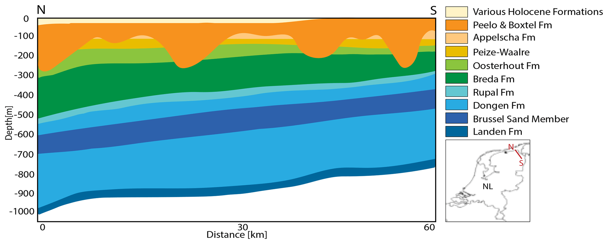
Figure 1Schematic cross section of the North Sea Group (NSG) based on formation depths from https://www.dinoloket.nl/ (last access: January 2020) and stratigraphic charts (Wong et al., 2007). The formations of the Lower NSG have blue colours, formations of the Middle NSG are in green, and Quaternary formations of the Upper NSG are in orange/yellow. From the different members in the Lower NSG, only the Brussel Sand Member is included due to its importance for this study.
The area of interest is the northeast of the province of Groningen, with a flat topography, close to mean sea level and a water table almost up to the surface. The sedimentary cover of interest is formed by the Cenozoic soft sediments, named the NSG, including the Upper, Middle and Lower North Sea groups (Fig. 1) (Vos, 2015). The top of the underlying Upper Cretaceous limestones (Chalk Group) is defined as a reference horizon in previous site response studies (Rodriguez-Marek et al., 2017) and recent seismic hazard models (Bommer et al., 2017; Kruiver et al., 2017).
The North Sea Group has an average thicknesses of about 800 m, with local variations in depth due to underlying salt diapirs and basin deepening towards the north. Paleogene and Neogene sediments mostly consist of transgressive marine clays alternated with continental siliciclastic sediments. At around 500–600 m depth, a high-velocity layer (Brussel Sand Member) of compacted sands is deposited during a phase of regression and subsequently partly eroded. Marine delta slope deposits consisting of clays and sands dominate the upper part of the North Sea Group, unconformably overlain by Quaternary glacial deposits (Wong et al., 2007). The Pleistocene sedimentary sequence is characterized by fluvial, aeolian, glacial and marine deposits that are crosscut by deep (down to 200 m) glacial tunnel valleys which are filled with sand and compacted clays, named the Peelo Formation. Very soft Holocene tidal channel sands, marine clays and peat form the upper 10–20 m of the Groningen subsurface (Meijles, 2015; Wong et al., 2007).
Kruiver et al. (2017) have built an integrated shear-wave velocity model for the Groningen area from the surface to the base of NSG. In this 3-D velocity model, large amounts of geological, geotechnical and geophysical observations are merged. Due to the rich data availability for the upper 40 m, the model is very detailed in this depth range (Noorlandt et al., 2018). At depths of 40–120 m, less detail is available as the velocity model is constrained through inversion of surface waves (recorded as noise) from reflection seismic surveys. Shear-wave velocities in the deepest part are derived from a pre-existing compressional-wave velocity model from reflection seismics and the conversion ratio is based on two borehole sonic logs (Zeerijp and Borgsweer). We refer to this velocity model as the Deltares-NAM model. Mainly for the deeper section of the NSG, the uncertainties are high for the shear-wave velocities since they are derived from a single Vp∕Vs ratio. Compressional-wave velocities show lateral heterogeneity. A conversion to shear-wave velocities away from the wells where the Vp∕Vs ratios were determined leads to errors. For accurate localization of the earthquakes, a shear-wave velocity profile for the Lower NSG for each station site is required.
Hofman et al. (2017) derived vertical seismic velocity profiles for both P and S waves for nearly all stations in the Groningen network, using seismic interferometry applied to local event data. Their method estimated velocities within four intervals from 0 to 200 m depth. These velocity models are in general in good agreement with the Deltares-NAM model, as is shown in Noorlandt et al. (2018). Our study benefits from this detailed shallow velocity structure for the upper 200 m of the North Sea Group, which we use to construct the velocity profiles at each of the seismic stations.
Spica et al. (2018) presented a comparison between the model from Kruiver et al. (2017) and velocities derived from the H∕V spectral ratio for the upper 200 m from 10 borehole stations in the Groningen network. Inversions of the H∕V spectral ratios based on the diffuse field assumption (Sánchez-Sesma et al., 2011) are developed to gather constraints on the shear-wave velocities. Subsequently, Spica et al. (2018b) assessed the velocity structure at 415 sites for a temporarily deployed dense surface array, covering only a small part of the Groningen gas field, through joint inversion of multimode Love- and Rayleigh-wave dispersion curves and H∕V spectral ratios. From this similar dense array, Chmiel et al. (2019) obtained shear-wave velocity models by using depth inversions of surface waves from ambient noise. They were able to derive velocities up to the base NSG by adding depth constraints to overcome weak sensitivities of surface waves at these depths. In summary, several high-resolution shear-wave velocity profiles across different scales became available over the last years for the Groningen area. Our findings complement available information on in situ velocity measurements at each seismic station in the Groningen network.
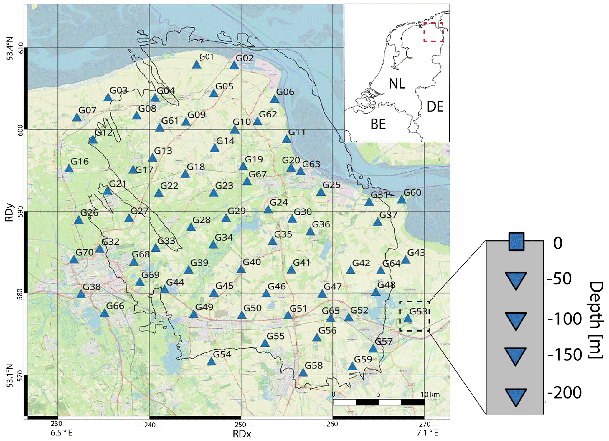
Figure 2Map view of the Groningen area. The triangles represent the surface location of the stations of the G-network. Each station contains an accelerometer at the surface (square) and four geophones at 50 m depth intervals (inverted triangles). Coordinates are shown within the Dutch National Triangulation Grid (Rijksdriehoekstelsel or RD) and lat/long coordinates in the corners for international referencing. Background map: © OpenStreetMap contributors, CC-BY-SA, https://www.openstreetmap.org/#map=6/51.330/10.453 (last access: October 2019).
Table 1List of teleseismic events used for this study. The epicentral distance and back azimuth are calculated for reference station G24.
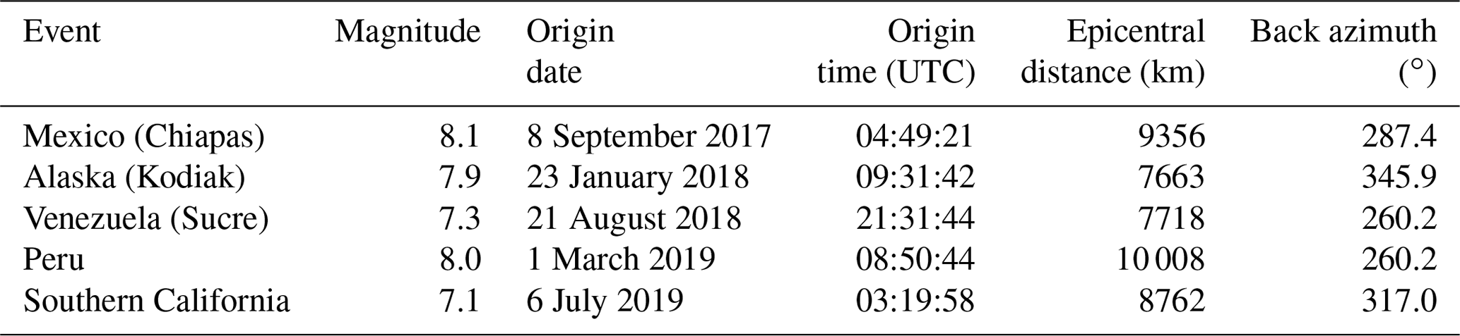
To conduct the present study, the Royal Netherlands Meteorological Institute (KNMI) shallow borehole network (further referred to as the G-network) was chosen, which has both borehole and surface seismographs. The G-network installed on top of the Groningen gas field consists of 69 stations (Dost et al., 2017) and Fig. 2 shows the distribution of the seismic stations in Groningen. Each station is equipped with three-component, 4.5 Hz seismometers at 50 m depth intervals (50, 100, 150, 200 m) and an accelerometer at the surface. The stations have been continuously recording since 2015 and the data are available via the data portal of Royal Netherlands Meteorological Institute (KNMI, 1993). We use a large three-component data set of ambient noise and five strong teleseismic events (Table 1) measured by the G-network. Several strong teleseismic events are required to obtain an estimate of the H∕V ratios and the standard deviation thereof. We refer to “station” for the entire string with one accelerometer and four geophones and refer to “seismometer” for a single sensor measurement at a certain depth. For calibration purposes, we use one broadband seismometer which is nearly co-located with one of the geophones.
Multiple strong (M > 7.0) global teleseismic phases are recorded within the G-network. Incoming body waves resonate between the free surface and the large impedance contrast between the soft-sediment layer and the seismic bedrock, resulting in amplification of both vertical and horizontal seismic motions. We assume that teleseismic S phases are transmitted into the NSG with angles smaller than 5∘ with vertical.
The size of the underlying impedance contrast determines how strongly the waves are reflected and thus how much of the wave energy is trapped. The interference of multiple reverberations within the soft layer leads to a resonance pattern in which certain frequencies are amplified and others interfere destructively.
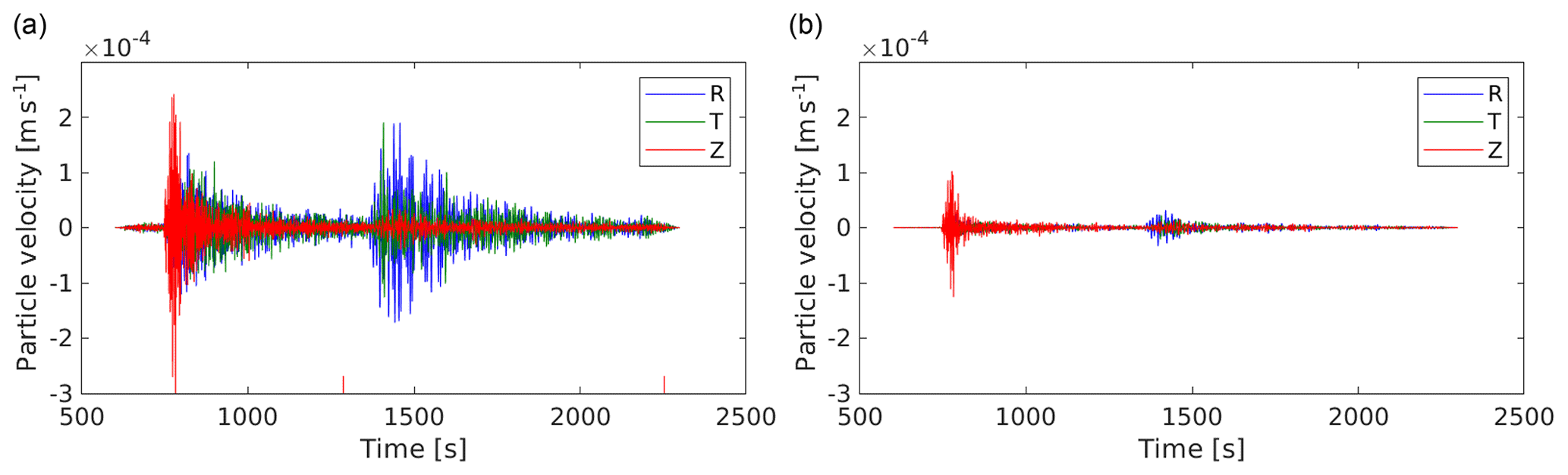
Figure 3Comparison of the Mexico M8.1 event (Table 1) recorded on (a) a soft-sediment site in Groningen (seismometer G300, epicentral distance 9359 km) and (b) at a hard-rock site (seismometer HGN, epicentral distance 9378 km) in the south of the Netherlands. R is the radial, T is the transverse, and Z is the vertical component of the seismometer. In panel (a), the red ticks indicate the 1000 s window. The direct P wave arrives at 750 s on the Z component, while the direct S wave arrives on the R and T components at 1400 s.
From five teleseismic arrivals, 1000 s time windows are taken, starting just prior the S-phase onset. The direct S phase, the later coda and the subsequent weaker shear-wave phases are included in this window. Figure 3 shows a seismogram for the Mexico M8.1 event for a soft-sedimentary site in Groningen and a hard-rock site in the south of the Netherlands. Both stations have a comparable distance to the event (9359 vs. 9378 km). A time window around the P phase and S phase is shown. Their amplitude is larger in Fig. 3a than in Fig. 3b mainly due to amplification over the soft sediments. Also, the basin setting for Fig. 3a leads to stronger coda. The response is band-pass filtered between 0.03 and 2 Hz. This is a low-frequency band for the equipped geophones and accelerometers. The lower part of this band, from 0.03 to about 0.2 Hz, is indeed most of the time dominated by instrumental noise. Strong teleseismic arrivals, however, are still well recorded down to 0.03 Hz. Their amplitudes are up to a factor of 1000 higher than the microseism. Events with magnitudes above 7.0 and with distances up to 90∘ produce S phases with sufficient energy to compute H∕V curves that contain resonances of the entire sedimentary sequence.
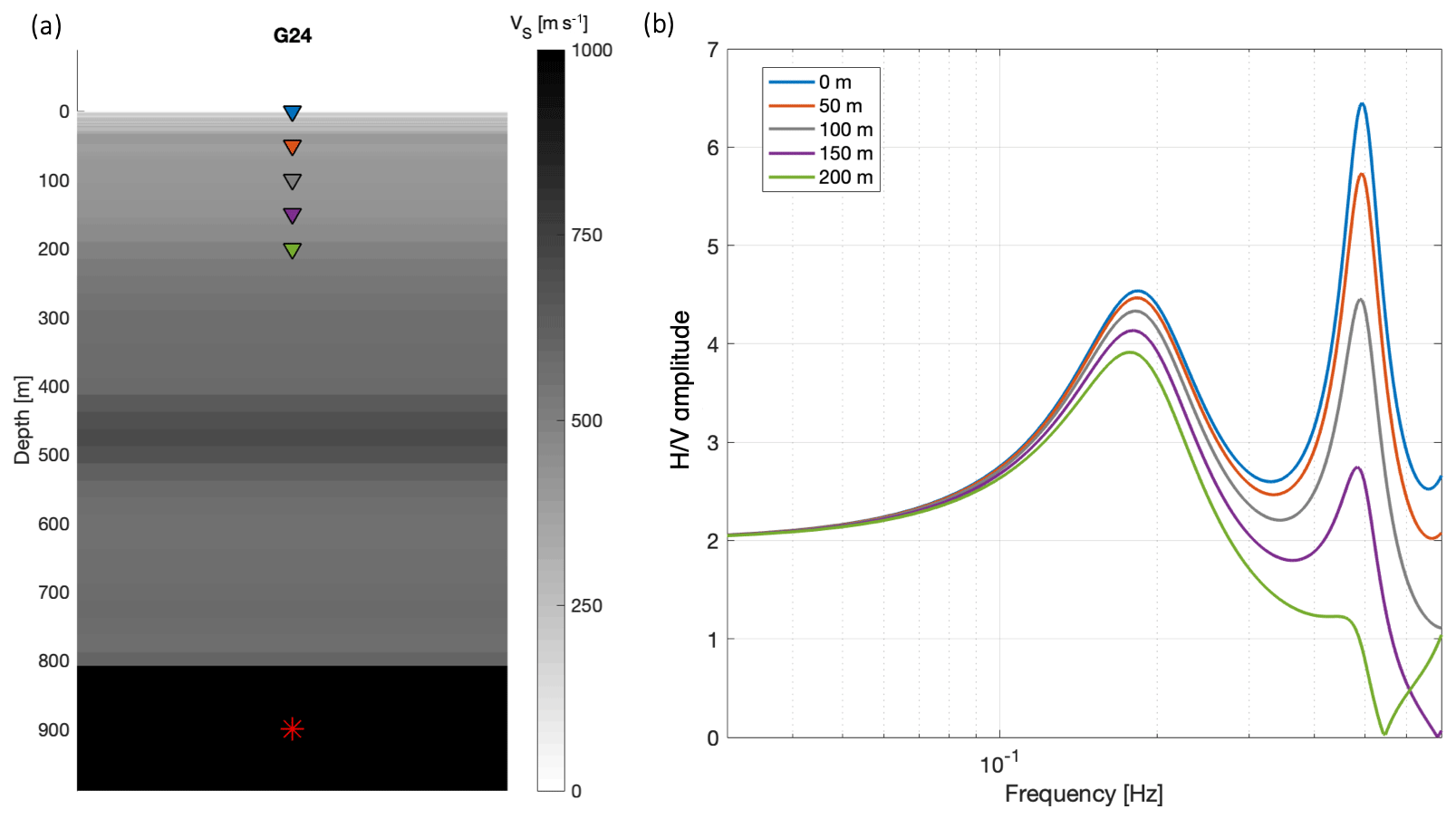
Figure 4(a) Velocity profile from the Deltares-NAM model at station G24. The top 800 m is made up of the NSG with much lower VS than the underlying Chalk Group. The coloured triangles denote instrumented depth levels, corresponding to the colours of the lines in (b). The red star indicates the depth of the synthetic source. (b) Forward-modelled amplitude spectra (coloured lines) for a vertically incident shear wave, recorded at the five different depth levels. Both the fundamental mode and first higher mode of the entire sedimentary column can be seen. Also, waves resonate between the free surface and the high-velocity layer at 450 m depth (Brussel Sand Member). The resulting fundamental mode interferes with the first higher mode of the entire NSG and results in the elevated peak just below 0.5 Hz.
5.1 Identification of resonance frequencies using teleseismic phases
Conventional H∕V curves are computed based on Fourier amplitude spectra (FAS; e.g. SESAME Project, 2004) or response spectra (Zhu et al., 2020). Here, we estimate H∕V curves from PSDs. We obtain the PSD by first estimating the FAS that we use in Eq. 1, which is the absolute value of the discrete Fourier transform: . Computing the PSD amounts to
where Δt is the sample duration and T the duration of the time window that was used to compute the FAS. The factor of 2 only needs to be applied when merely positive frequencies are used. The PSD is a frequency-normalized version of the power spectrum, which makes the spectrum less sensitive to input data duration T (Havskov and Alguacil, 2004). Our main reason to start off with PSDs instead of FAS is that PSDs are already routinely computed for data inspection and quality checking purposes (McNamara and Buland, 2004). In the computation of PSDs, we follow the recipe of Peterson (1993) which results in well-averaged spectra, which is elementary for usage in H∕V computation. A large difference with typical PSD computations is that we do not apply any smoothing. From a 1000 s window, starting just prior to the S-phase arrival (Fig. 3), PSDs are computed using time windows of 102.4 s with a 75 % overlap (Peterson, 1993). The two horizontal components are averaged by vector summation and subsequently the horizontal-to-vertical ratio is taken from the PSDs, resulting in the body-wave H∕V ratio (HVBW):
where the subscripts E, N and Z denote the east, north and vertical components, respectively. When substituting Eq. (1) into the above equation, one finds that the PSD-based HVBW is consistent with a FAS-based H∕V computation:
in which the FAS of both horizontal components is combined through vector summation. No smoothing is applied since smoothing will affect the picking of the exact fundamental resonance peak. For sites with multiple significant peaks, smoothing could result in a shift to higher frequencies and a bias in identification of the fundamental resonance peak (Zhu et al., 2020). Albarello and Lunedei (2013) present several alternative procedures to average the horizontal components for computing ambient noise H∕V ratios and conclude that vector summation is the most physically logic averaging method; therefore, this averaging procedure has been applied to the two horizontal-component PSDs. Nevertheless, we tested the different methods and found no difference in resulting peak frequencies for our data set, but biases may arise between the different averaging methods when evaluating the amplitude of the H∕V peak (Albarello and Lunedei, 2013).
A synthetic test shows that the borehole seismometers across different depths measure the same fundamental resonance (f0) of the entire soft-sedimentary column. An example is shown in Fig. 4 for the Deltares-NAM model at station G24. The H∕V amplitude at f0=0.18 Hz does vary over the different depth levels. The instruments at depth experience notches due to interference of upward- and downward-propagating waves. For larger depths, the notches shift to lower frequencies; in Fig. 4, the first notch for the 200 m depth instrument can be identified at 0.55 Hz. The interference of the notch with f0 leads also to a shift in frequency. Since the frequency perturbation is less than 0.01 Hz, it is decided to calculate the mean HVBW over all depth levels to better cancel out noise and to obtain a more stable result for picking f0.
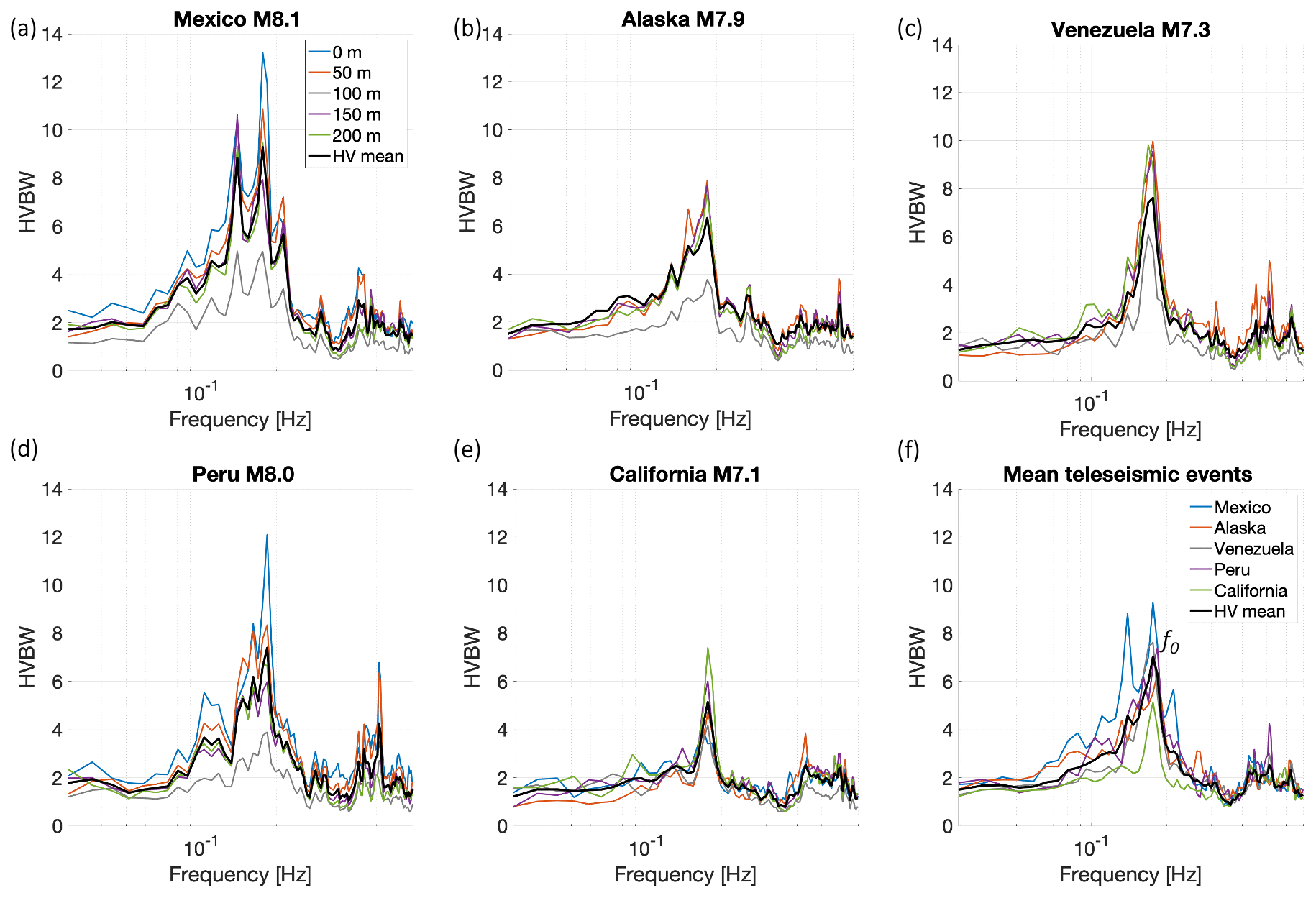
Figure 5HVBWs from five teleseismic events recorded at station G24: (a) Mexico (M8.1), (b) Alaska (M7.9), (c) Venezuela (M7.3), (d) Peru (M8.0) and (e) southern California (M7.1). The coloured lines show the HVBW curves at different depth levels; the black lines show the average per event. (f) From the five mean HVBWs (black lines in panels a–e), a second averaging is performed to estimate the final HVBW for this station. The black line is the calculated mean HVBW over the five event HVBWs (coloured lines). The peak frequency of the mean HVBW (f0) is picked for shear-wave velocity calculations using Eq. (4).
We compute the HVBWs (Eq. 2) for five teleseismic arrivals (Table 1). Figure 5 shows example HVBW curves for station G24. Note that, though the amplitudes are slightly different, the frequency of the main peak (f0) is consistent from event to event. Frequencies above 0.7 Hz are omitted since the S phase provides insufficient energy above this frequency threshold. By applying the H∕V method to teleseismic phases, the source and path effect are largely suppressed to focus on the site effect. However, this suppression is always incomplete. Furthermore, we assume vertical incidence but in reality this is not obtained. These two facts explain the difference in amplitudes of the resonance peak for each event, despite the uniform subsurface. Some HVBW curves show multiple peaks near the f0 (Fig. 5a, d), causing a challenge to distinguish the peak corresponding to the resonance of the entire North Sea Group. Comparing HVBW curves from different events helps to pick the peak belonging to the fundamental resonance frequency, and by averaging over multiple events, the error in the mean f0 is minimized.
5.2 Calculating shear-wave velocities
From the HVBW, we interpret the prominent low-frequency peak at 0.18 Hz as the fundamental shear-wave resonance frequency (f0) of the complete NSG package. From each HVBW peak (f0), shear-wave velocities can be calculated based on (Tsai, 1970), assuming vertically incident body waves and assuming a known thickness of the resonating layer d:
where f0 represents the fundamental resonance frequency, Vs is the (harmonically averaged) shear-wave velocity from surface to the bedrock interface, and d the depth of the base of the NSG. Since the depth of the NSG is accurately defined from 3-D reflection seismics in combination with lithostratigraphic marks of hundreds of boreholes (Van Dalfsen et al., 2006; Kruiver et al., 2017), the shear-wave velocity is straightforwardly calculated. Per station and for each teleseismic event, the velocity is calculated with Eq. (4), and subsequently the five shear-wave velocities are averaged. This averaged shear-wave velocity for each station is referred to as and is plotted in Fig. 6a. Stations G45 and G52 are discarded, due to the scattering effect of the underlying salt domes, the local 1-D assumption is here not valid to calculate velocities using Eq. (4). After all, shear-wave velocities are calculated at 63 stations .
Hofman et al. (2017) have constructed detailed shear-wave velocity profiles of the upper 200 m at G-network stations (). The teleseismic velocity profiles () give velocities for the complete NSG. Per station, an estimate of the average S-wave velocity of the Lower NSG () is obtained by combining the and estimates using
which corresponds to harmonic de-averaging. This calculation is done for each station (Fig. 6b), where zNSG represents the thickness of the entire NSG and zNSL the thickness of the lower part of the NSG. Figure 7 shows four examples of velocity profiles constructed with this method. The seismic velocity of the Chalk Group is based on well logs in Zeerijp and Borgsweer. For each station, these profiles are used as input for forward modelling (Sect. 7).
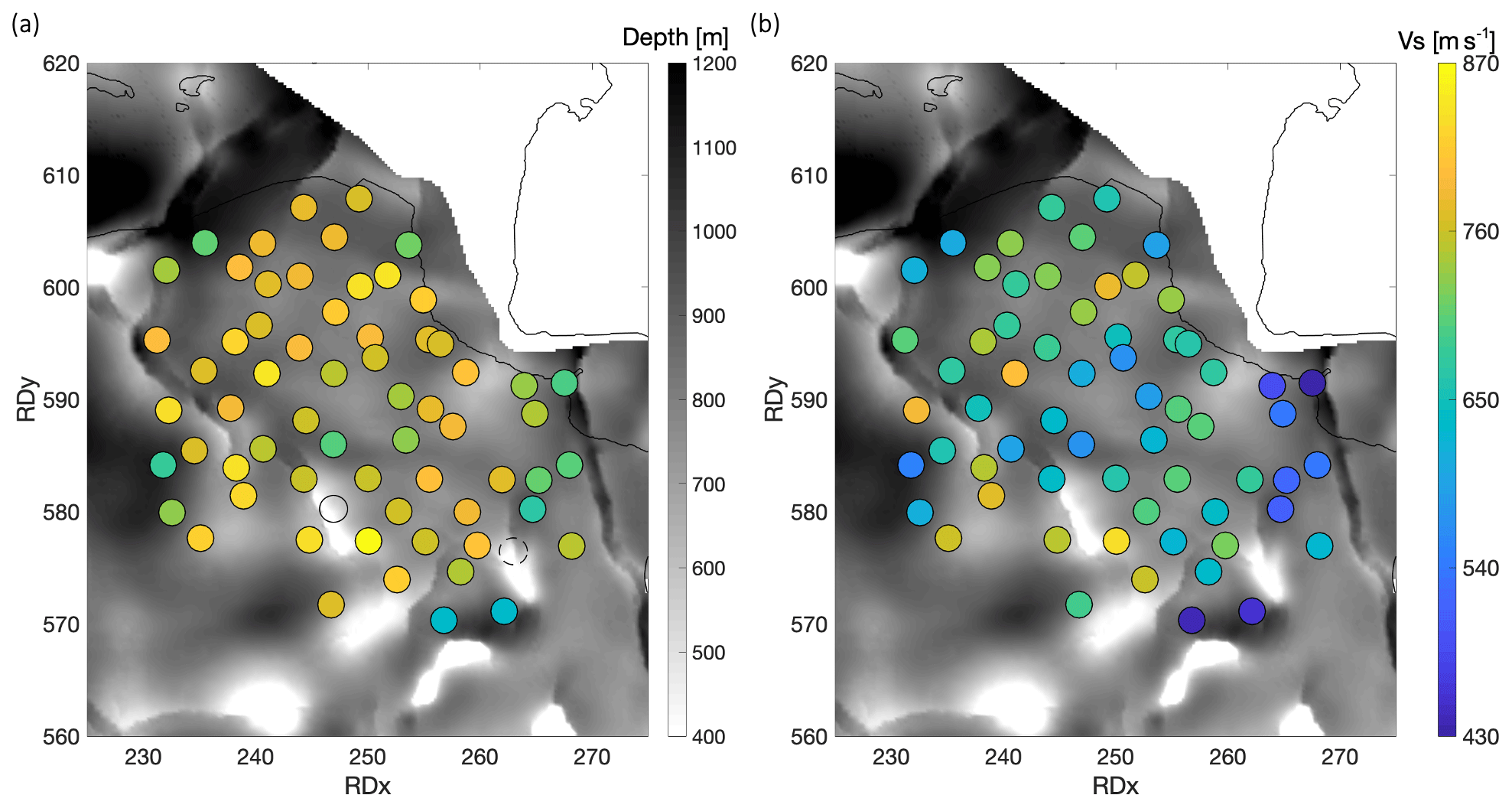
Figure 6Average shear-wave velocities for the North Sea Group from each station in the Groningen network. Coordinates are plotted in RD projection. (a) Map of the depth of base North Sea Group (Van Dalfsen et al., 2006) with, in circles, the average shear-wave velocities for the entire North Sea Group (). The solid circle represents discarded station G45 and the dashed circle represents discarded station G52. (b) Average shear-wave velocities calculated according to Eq. (5) for the lower part of the NSG (): from 200 m depth to the base of the sedimentary cover.
For all stations, the standard deviation of the average over five teleseismic events is calculated and plotted in Fig. 8a. This figure shows the variation of the estimated velocity over the 63 sites. If we leave out the outliers (G58 and G59), we get an average shear-wave velocity and standard deviation of over Groningen of 526 and 31 m s−1, respectively. For , the average velocity and the standard deviation are 637 and 59 m s−1, respectively (Fig. 8b). Higher standard deviations for can be explained by the same error being attributed to only the Lower NSG instead of the entire NSG.
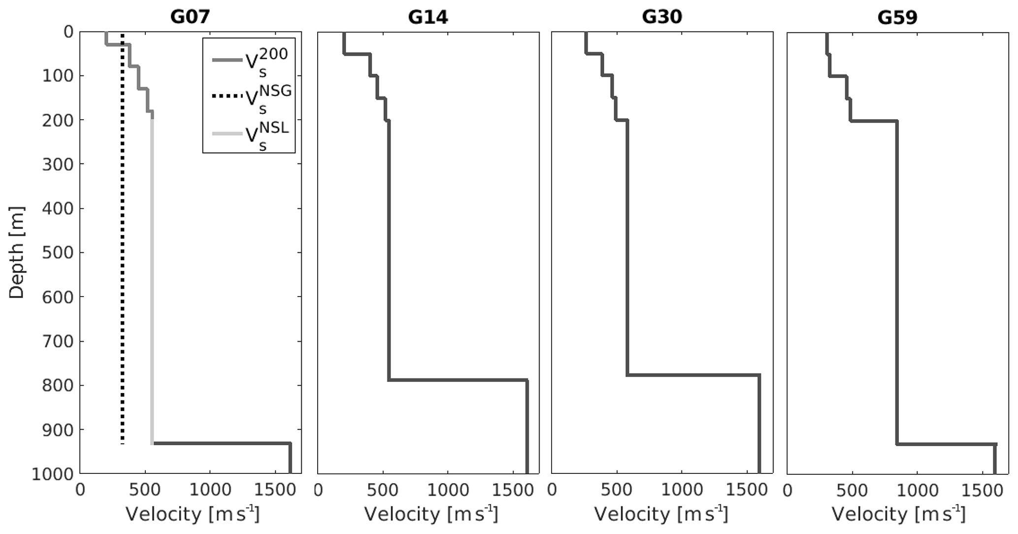
Figure 7Final subsurface velocity profiles, respectively, for stations G07, G14, G30 and G59. The left panel shows the construction of a merged shear-wave profile: velocity profiles of the upper 200 m (, dark grey line) are taken from Hofman et al. (2017); the entire NSG average velocity (, dotted line) is taken from teleseismic phases. (light grey line) is calculated from and (Eq. 5). The velocity contrast at around 800 m depth is between the base NSG and top Chalk Group.
5.3 Calculating an empirical bedrock–depth function
In the previous section, we took advantage of the well-constrained depth of the unconsolidated sediments to invert for shear-wave velocity. In other areas in the Netherlands, similar sedimentary fills exist, but the depth of the NSG is less well constrained. Some areas have depth constraints from deep wells in the area, but much fewer exist than in Groningen. Other areas rely on reflection seismic data and again other areas have neither of the two. Alternatively to using Eq. (4) together with an average NSG shear-wave velocity as found in the previous section, we first use the large data set available for the Groningen area to establish a frequency–depth relationship by finding an empirical relation connecting depth d with resonance frequency f0 in the form of
as introduced by Ibs-von Seht and Wohlenberg (1999). In the particular case of a lossless single-resonating wave assumption, the factors a and b in Eq. (6) correspond to Vs∕4 and −1, respectively (Eq. 4).
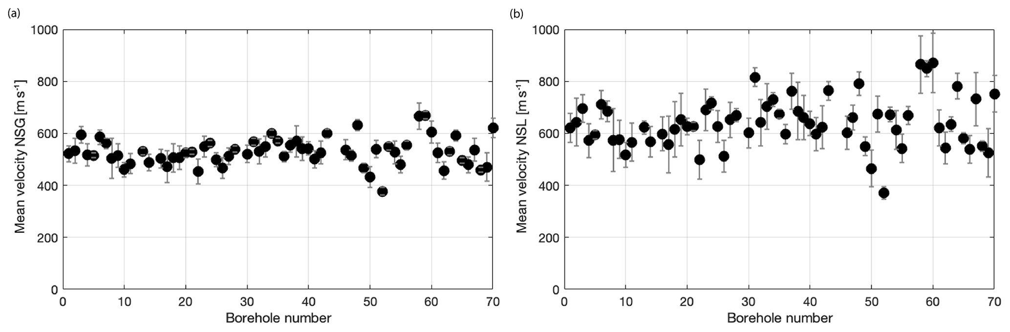
Figure 8(a) Average shear-wave velocities (black dots) and standard deviation (grey bars) derived from the H∕V ratio of five teleseismic events, sorted by station number for (a) and (b) .
Figure 9 shows the f0–depth distribution and least-squares fit of Eq. (6), yielding as a mean model for the NSG sediments:
and a depth standard deviation of 73 m. Using the mean depth of the data set (814 m), this corresponds to a standard deviation of 9 %. For comparison, the model that Ibs-von Seht and Wohlenberg (1999) found in the Aachen area (Germany) is shown. Clearly, using the latter model would yield a too-deep sedimentary fill for the Netherlands. Here, we show that the sedimentary setting in the Netherlands is different from fitted models around the world, as summarized in Thabet (2019), leading to different values for a and b. The marine and clay-rich sediments of the NSG are of a very young age; therefore, less compaction has strengthened the material. The newly established relationship can be used to estimate the sediment thickness for the NSG where the geology is similar.
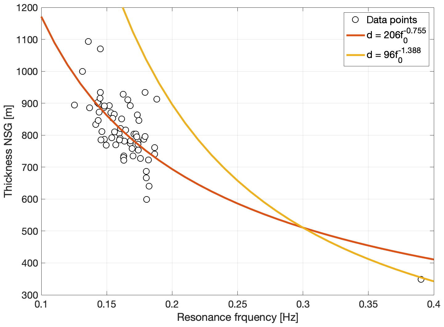
Figure 9The thickness of NSG versus fundamental resonance frequency f0 distribution for 63 sites in Groningen (black circles), together with the least-squares fitted function (orange line) and the empirical model for the Aachen region (yellow line) as obtained by Ibs-von Seht and Wohlenberg (1999).
The majority of studies on H∕V spectral ratios are based on recordings of the ambient noise field. In this section, we estimate the H∕V spectral ratios using the ambient noise wave field. Multiple years of ambient noise recordings are available, and to obtain stable H∕V ratios we employ a sequence of averaging procedures as outlined below. In the next section, the obtained results are compared with modelled H∕V spectral ratios. For the H∕V modelling, we use the Geopsy gpell algorithm for surface waves and the velocity profiles derived in Sect. 5. This enables us to quality check the H∕V method applied to teleseismic arrivals.

Figure 10Probability density functions (PDFs) from ambient noise horizontal-to-vertical spectral ratios (HVAN) for station G39, 50 m level. The black line represents the mean. (a) HVAN PDF for 1 week (21–28 March 2017). (b) HVAN PDF for 1 month (1 May–1 June 2017). (c) HVAN PDF for 1 year (1 February 2017–1 February 2018).
Similar to the teleseismic recordings, power spectral densities (PSDs) are calculated from ambient noise data for all three components for the 50 m depth seismometers in the G-network. The 1 d ambient noise records are divided into time windows, and for each time frame the PSD (Eq. 1) is calculated, using 75 % overlapping time segments. Each segment is 214 time samples (82 s) long. Subsequently, for each day, an H∕V ratio is computed from the PSDs by implementing Eq. (2). In McNamara and Buland (2004), the probability density function (PDF) of the PSD is computed. This allows separating long-term noise conditions from transient events and time periods with sensor malfunctioning. We follow an approach similar to the one in McNamara and Buland (2004), but instead of a PDF of the PSD, we compute a PDF of the ambient noise H∕V ratios. We further refer to this distribution as PDFs of H∕V spectral ratios of the ambient noise (HVAN). Figure 10 shows examples of the HVAN PDF for station G39 for multiple recording durations. In a conventional H∕V plot, there would be a mean H∕V value for each frequency, or a mean value and a confidence zone, based on a normally distributed error model. Instead, the PDF shows the complete digitized H∕V probability distribution for each frequency. From this distribution, the mean, mode, median and different percentiles can be taken.
Generally, H∕V estimations are based on noise measurements of largely varying duration: for less than 1 h (e.g. Fäh et al., 2001; Scherbaum et al., 2003), a few days (e.g. Ruigrok et al., 2012) or up to a month (e.g. Parolai et al., 2002). Due to the permanent deployment of the network in Groningen, noise has been recorded for almost 3 years. This creates an excellent opportunity to test what minimum window of noise data yields a stable H∕V curve. Furthermore, by measuring a long period of noise, the HVAN can be expressed as a PDF for any desired period for each seismometer in the network. Figure 10 shows distribution plots of, respectively, 1 week, 1 month and 1 year of the calculated HVAN PDF. A stable peak around 0.4 Hz is created by at least 1 month of recording of the ambient noise field. This 1 month is the preferred duration because of manageable data handling instead of a year of data. Therefore, for all stations at 50 m depth, 1 month of ambient noise data is used to compute the HVAN PDF. From this distribution, the mean HVAN is extracted. This HVAN is likely descriptive of the site, rather than a remnant of source or path effects.
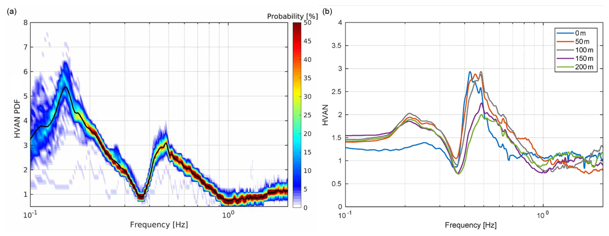
Figure 11(a) HVAN PDF for 1 month (1 September–1 October 2018) at broadband station G82B, located within 100 m of G39, with a depth of 100 m. The broadband HVAN PDF displays a peak for the fundamental mode (around 0.15 Hz) and the secondary peak (around 0.45 Hz) reflects the higher mode for Rayleigh waves or the presence of a second strong impedance contrast. The black line indicates the mean from the HVAN PDF. (b) HVAN curves for 1 month for station G39 for all depth levels.
For the 4.5 Hz seismometers in the G-network, instrument noise is dominating frequencies below 0.2 Hz, where also the fundamental mode of the NSG resonance is expected. Due to large storms across the year, in which the microseism noise surpasses the instrumental noise, the computed HVAN PDF for 1 year (Fig. 10c) shows a peak around the fundamental resonance frequency (0.15 Hz) of the NSG. In the case of an energetic ocean state, the amplitudes in the fundamental mode are similar to the higher mode peak. However, over the year, the probability is low and picking the corresponding peak frequency is unreliable. In August 2018, four broadband seismometers were installed in Groningen at 100 m depth. With these broadband data, we are able to confirm the recordings of the fundamental mode of the NSG. Figure 11a shows the HVAN PDF for broadband station G82B which does have a clearly resolved peak for the fundamental frequency. Due to the unreliability of the fundamental mode peak in the G-network geophones and accelerometers, in the following we focus on the subsequent notch, between 0.3 and 0.4 Hz (Fig. 10).
Triggered by a study by Lontsi et al. (2015), the depth dependency of the H∕V curve across a downhole array is evaluated in Fig. 11b. With increasing seismometer depth, a maximum shift (0.06 Hz) of the higher-mode peak is observed. For the surface accelerometer, nearly all ground motion falls outside its dynamic range, below 0.3 Hz. The instrumental noise has the same level on all 3 components. As a consequence, the H∕V ratio is close to 1 below 0.3 Hz, whereas the geophones still have a small sensitivity down to 0.2 Hz. The remaining pattern of the H∕V curves in Fig. 11 are consistent with Fig. 3b, where the body-wave H∕V amplitude is decreasing as function of depth. Here, we use the seismometer at 50 m depth, where anthropogenic noise is considerably less than at the Earth's surface, and hence a more stable HVAN can be computed. The software (Geopsy gpell) used for forward modelling assumes measurements at the surface; therefore, the 50 m depth station is preferred over the deeper levels.
Commonly, the ambient seismic field is dominated by surface waves (Aki and Richards, 2002; Bonnefoy-Claudet et al., 2006a, b). Ocean-generated seismic noise (microseism) is measured on the Groningen seismometers from ∼0.1 to 1.0 Hz. Here, the low-frequency ambient seismic field is composed of microseisms induced by Atlantic Ocean gravity waves, while the higher frequencies are mainly induced by North Sea gravity waves. Both sources have a main propagation direction from the northwest (Spica et al., 2018a; Kimman et al., 2012). Spica et al. (2018b) discuss the wave field in Groningen up to 0.6 Hz and conclude that the H∕V peak around 0.15 Hz is dominated by Rayleigh waves and the H∕V peak around 0.4 Hz by body waves. Moreover, a review of Lunedei and Malischewsky (2015) expresses the view that H∕V curves are composed by the whole ambient-vibration wave field, although not in equally distributed proportions. To better understand the measured H∕V curves and to create a perspective on the composition of the microseismic ambient noise field, we perform both body-wave forward modelling (shear-wave resonance) and surface-wave forward modelling (Rayleigh-wave ellipticity).
.
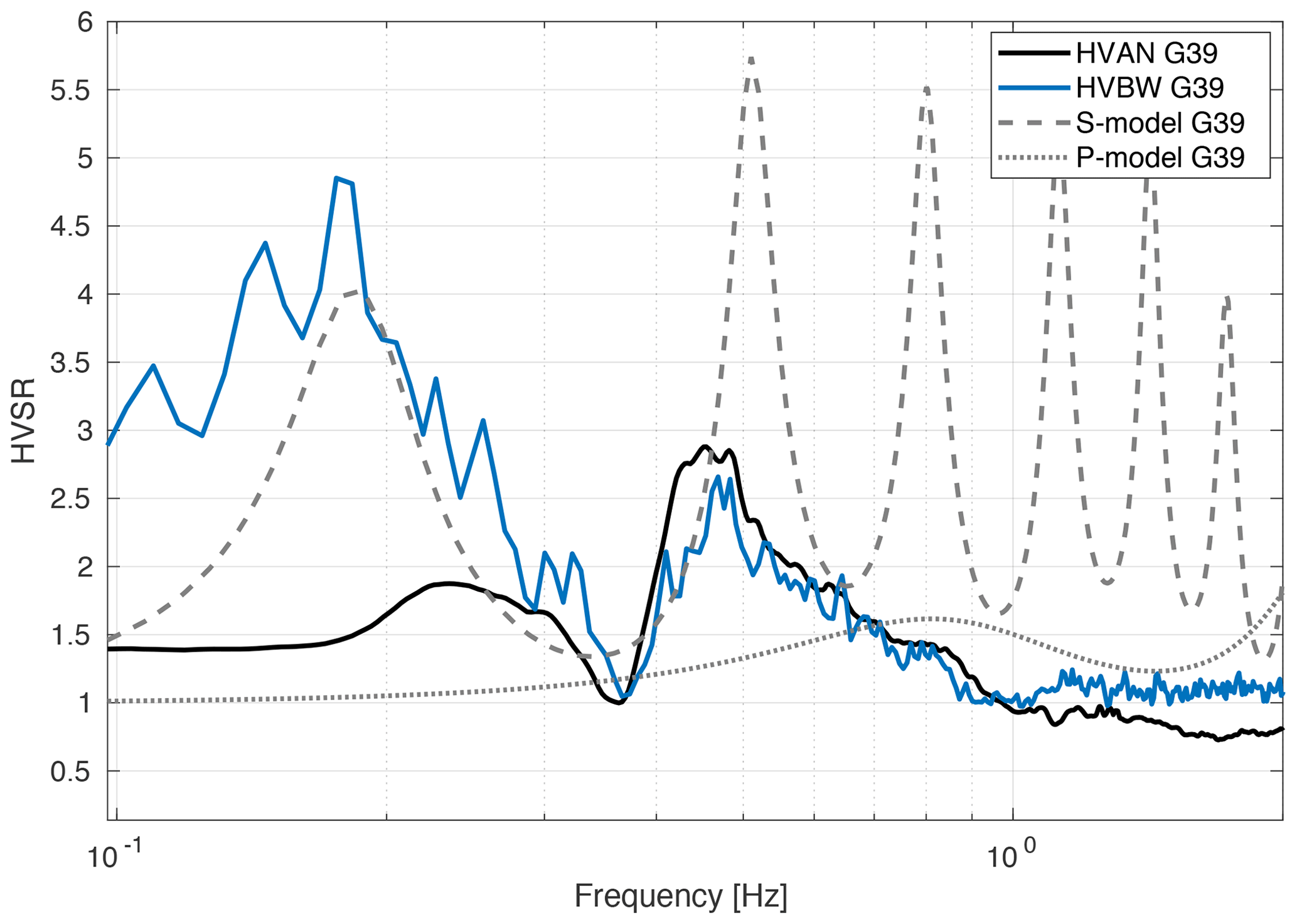
Figure 12Modelled shear-wave resonance (dashed line), compressional-wave resonance (dotted line), HVAN (black solid line) and HVBW (blue solid line) for the 50 m depth seismometer of station G39. The HVBW is taken as the mean over five teleseismic phases (Table 1).
7.1 Body-wave forward modelling
Body-wave forward modelling is performed using OpenHVSR, developed by Bignardi et al. (2016). This software computes theoretical transfer functions of layered soil models based on the fast recursive algorithm from Tsai (1970). For the forward model input files, we use the subsurface shear-wave velocity profiles as described in Sect. 5. To the five layers over a half-space velocity model, we add also a five-layer seismic quality factor. Q values of, respectively, 10, 50, 50, 50 and 100 are determined from the borehole stations. Compressional-wave velocities are derived from existing velocity models (Van Dalfsen et al., 2006). The body-wave forward model (Fig. 12) shows modelled shear- and compressional-wave resonance spectra and is combined with the HVAN curve and the HVBW from station G39. The fundamental frequency for the HVBW has quite a good fit with the modelled body-wave resonance.
7.2 Ellipticity forward modelling
Next to body-wave forward modelling, we apply a forward modelling tool for surface waves (Rayleigh waves) to further investigate the wave field composition. Rayleigh waves exhibit an elliptical particle motion confined to the radial–vertical plane (Aki and Richards, 2002). Many studies have shown that the H∕V ratio of ambient noise is related to the amplitude ratio of the radial component of the Rayleigh wave over its vertical component (Arai and Tokimatsu, 2004; Bard, 1999; Bonnefoy-Claudet et al., 2006a; Konno and Ohmachi, 1998; Lachetl and Bard, 1994; Maranò et al., 2012, 2017) and that the H∕V ratio does not depend on the source or the path of the Rayleigh wave, but it depends only on the structure beneath the receiving station (Ferreira and Woodhouse, 2007a, b). Rayleigh-wave ellipticity is frequency dependent in the case of a layered and more complex subsurface. In the case of a strong impedance contrast of a factor of 2.5–3.0, the ellipticity curve shows singularities where the energy of the vertical component vanishes (Wathelet, 2005). In theory, this results in a singular peak at the fundamental resonance frequency and a singular trough at higher frequency (SESAME Project, 2004; Malischewsky and Scherbaum, 2004; Malischewsky et al., 2006). In practice, no full singularities are obtained since the recordings never purely contain Rayleigh waves.
The acquired subsurface shear-wave velocity profiles (Sect. 5) based on teleseismic arrivals, are used as input for Rayleigh-wave forward modelling, using the gpell module in Geopsy (Wathelet et al., 2008). Velocities from the half space (Chalk Group) are derived by averaging sonic logs from the wells of Zeerijp and Borgsweer (Kruiver et al., 2017), which are assumed to be constant over the area. We perform several tests to investigate the sensitivity for properties of the reference horizon (Malischewsky and Scherbaum, 2004), shear- and compressional-wave velocity variations, single and multiple velocity layers over a half space, and the presence of a high-velocity layer representing the Brussel Sand Member. These variations are of minor impact on the resulting ellipticity curves.
Since instrument noise dominates in the frequencies below 0.2 Hz, the fundamental peak of the ellipticity curves cannot be compared to the HVAN of the seismometers in the G-network. According to Maranò et al. (2012), the ellipticity of the fundamental mode exhibits not only a peak at the fundamental resonance frequency (f0) but also a trough at higher frequencies corresponding to changes in particle motion. In the HVAN curve, a trough is well expressed and can be linked to the trough of the ellipticity fundamental mode, while the first and second higher modes are hidden in the wide peak around 0.4 Hz and cannot be distinguished as single peaks in the HVAN (Fig. 13a).
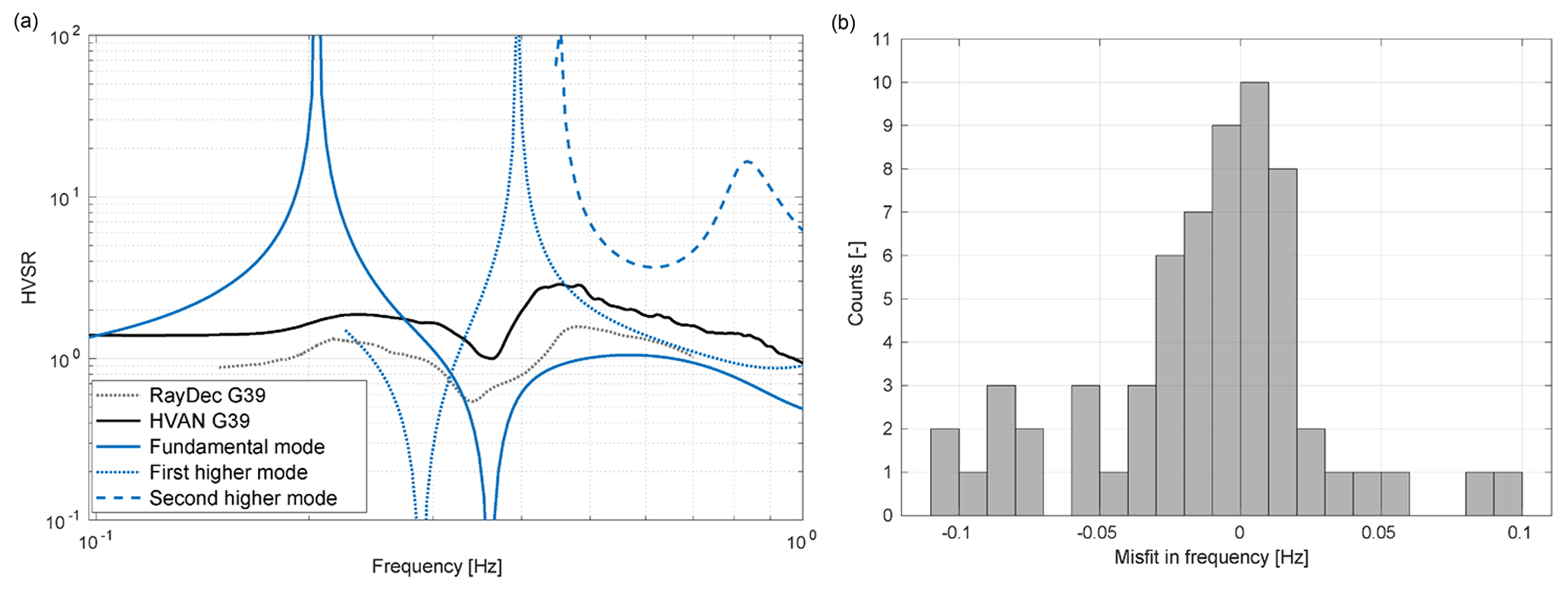
Figure 13For all stations, the difference is determined between the trough of the HVAN at low frequencies and the negative singularity of the fundamental mode of the Rayleigh ellipticities. (a) Example of Rayleigh-wave ellipticity curve for fundamental mode (blue line), first higher mode (dotted blue line) and second higher mode (dashed blue line), HVAN curve (black line) and RayDec (grey dotted line) for station G39. (b) Misfit between the troughs of the modelled ellipticity and the HVAN for all stations in the G-network.
The misfit between the troughs of the fundamental-mode HVAN and modelled ellipticity is presented in Fig. 13b. The majority of the stations are within the ≤0.03 Hz error range. The mean misfit is about zero, which indicates that the computation of HVBW and the further extraction of velocity profiles (Sect. 5) has not introduced a bias. From the overall good fit between the HVAN curves and ellipticity troughs of the fundamental mode, we can conclude that the input subsurface shear-wave velocity model is on average consistent with the measured ellipticity troughs of HVAN.
Hobiger et al. (2009) developed RayDec, a method enabling Rayleigh-wave ellipticity to be extracted from the ambient noise based on the random decrement technique. We applied this method and compared the result with the HVAN curve and modelled ellipticity curves. In RayDec, the signal of each time window is projected in the direction of dominant polarization. This azimuth depends on the time-varying and frequency-dependent noise field. Thus, for a successful application of RayDec, it is necessary to use small time windows and split up the larger-frequency band in different bins. For site G39, the RayDec curve does show a trough close to the HVAN minimum (Fig. 13a); therefore, this technique confirms that this trough can be attributed to Rayleigh-wave ellipticity.
7.3 Ambient noise field composition
Body-wave (Fig. 12) and surface-wave (Fig. 13) forward modelling results are compared with HVAN to determine the ambient wave-field composition. It can be noted that there is a small offset in peak frequency between the shear-wave resonance peak for body waves (close to 0.19 Hz) and the ellipticity peak for surface waves (around 0.2 Hz). With an impedance contrast around a factor of 2.5–3.0 between the NSG and the Chalk Group, the offset between the fundamental resonance frequency and ellipticity notch is consistent with the observations from Wathelet (2005). The HVAN (black line in Fig. 12) shows a large similarity to the HVBW observed at G39 (blue line) between 0.4 and 1.0 Hz. This indicates that there is a prominent body-wave presence in the ambient noise, for the investigated frequency range, which corresponds with findings of Spica et al. (2018a) and Brenguier et al. (2020). At the same time, there is a surface-wave presence, because Fokker and Ruigrok (2019) and Mordret et al. (2020) retrieved Rayleigh waves in this band, using noise recordings from the G-network.
The trough between 0.2 and 0.4 Hz on the HVAN curve is not well developed in the modelled shear-wave resonance (dashed grey line in Fig. 12). It shows more similarities with the notch in the ellipticity (blue line in Fig. 13). With RayDec, it was confirmed that there is indeed a Rayleigh-wave presence in this frequency band. This observation is supported by Kimman et al. (2012), who used a broad-band array in the Groningen area and found well-pickable phase velocities for Rayleigh waves between 0.2 and 0.4 Hz. Interestingly, a similar ellipticity trough can be seen in the HVAN curve (Fig. 12). This means that there must also be a (minor) contribution of Rayleigh waves in the teleseismic phases, in order to explain a similar notch. Direct Rayleigh waves will be largely attenuated at 0.3 Hz over teleseismic distances. Thus, the Rayleigh-wave presence is likely in the coda of S phases due to conversions in or near the sedimentary sequence.
In this paper, we present a method to establish a shear-wave velocity profile for the NSG sedimentary layer, based on five teleseismic events at each station location of the Groningen borehole network. Subsequently, velocity profiles for the lower part of the NSG are constructed. These velocity profiles are used as input for body- and surface-wave forward modelling and compared to the HVAN to determine the wave-field composition. Moreover, we have validated the new shear-wave velocity profiles by comparing HVAN curves to the theoretical Rayleigh-wave ellipticity curves in the band where Rayleigh waves dominate. On average, there is a good match between the two. However, locally there are inconsistencies between the HVAN and HVBW results. In this section, we make a comparison with the existing velocity model of Deltares-NAM and discuss uncertainties and limitations of our approach.
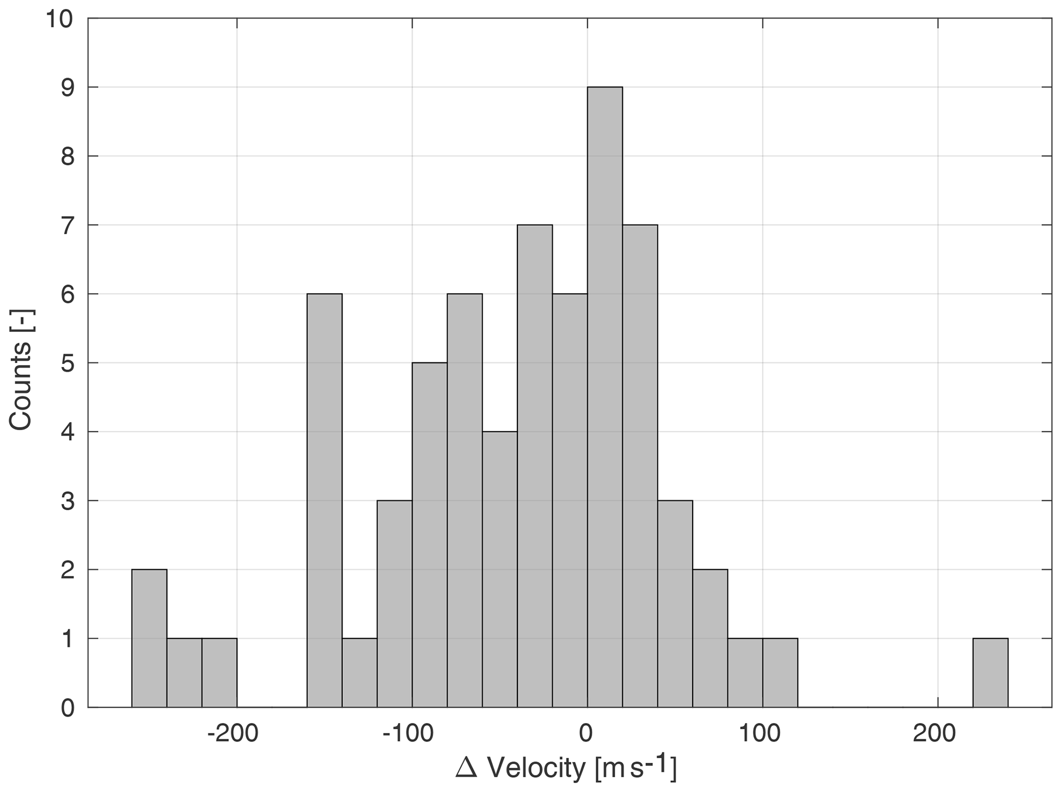
Figure 14Histogram of the misfit between the Deltares-NAM velocity model (Kruiver et al., 2017) and the velocity profiles for the lower part of the North Sea Group () presented in this paper. A count with a positive misfit corresponds to a station location with higher velocities in the Deltares-NAM model.
The new shear-wave velocity profile for each station location is compared with the Deltares-NAM model (Fig. 14), which is constructed using fixed Vp∕Vs ratios over the Groningen area, and thus local lithological variations that affect Vs differently than Vp are not accounted for. By using direct measurements of teleseismic phases per station, local subsurface variations are directly translated into average shear-wave velocities, which can explain the differences in velocities between the Deltares-NAM model and our model. The mean shear-wave velocity difference between the two models is −48 m s−1. This negative mean difference means that HVBW derived velocities are in general higher than the Deltares-NAM velocities. The majority of the stations have less than 100 m s−1 difference in shear-wave velocity between the two models. Stations G58 and G59 represent the highest misfit in velocities because of the exceptional high that we found.
As for most unconsolidated sediments, in Groningen, Vs increases with depth, which results in surface waves showing their normal dispersive behaviour, meaning that lower frequencies propagate faster. When Eq. (4) is used for finding the depth of these normally dispersive sediments, Bignardi (2017) showed that the depth is underestimated. Also we found, when modelling the resonance of a complex Groningen NSG model (Fig. 4), that f0 is larger than in the case of a single layer with the same harmonic average as the sequence of layers. In the normally dispersive multi-layer case, the part of the wave field that already reflects before reaching the free surface interferes with the free surface reflection, leading to an increase of the combined f0. The shift of f0 is small and highly dependent on the near-surface model that is assumed. Nevertheless, using Eq. (4), a larger f0 results in underestimation of the depth. Similarly, when using Eq. (4) for finding an average Vs when the depth is known, a larger f0 leads to an overestimation of the velocity. This finding is consistent – on average – with the overestimation of the velocity that we obtain with respect to the Deltares-NAM model.
Other assumptions that underlie Eq. (4) are that there are no losses and vertically incident body waves. Though f0 goes up for a more realistic layering, f0 goes down again when realistic losses are added to the model. Moreover, f0 would further be reduced if a correction was made for the non-vertical incidence of the teleseismic phases, which were used for computing the HVBW. Since the exact corrections are unknown, it is not straightforward to make these corrections. On average, we measure higher shear-wave velocities than the Deltares-NAM model, and this inconsistency might imply the dominant effect of multi-layer interference that is not incorporated in this model.
Finally, it has been assumed that a local 1-D approximation can be made. The main impedance contrast is the base of the NSG, which is laterally smoothly varying over the region. This supports a local 1-D assumption for each individual borehole station. Two stations at flanks of salt domes have been excluded from the analysis because of possible 3-D effects.
In the near future, the updated Vs model will be tested for hypocentre localization with the Groningen network. Because of the above considerations, it is expected that there is a bias in the absolute values, but that the lateral variations of Vs are quite well resolved.
We computed probability density functions of the ambient noise H∕V prior to extracting an average. Knowing this H∕V distribution, a tailored averaging procedure can be taken to obtain a non-biased H∕V estimate. For example, to exclude the influence of outliers, first the 95 % confidence zone of the H∕V distribution can be selected, and subsequently the mean of this distribution can be taken. In the case of a bi-modal distribution, one of the distributions is often pertaining to the actual resonance characteristics of the site, whereas the other might correspond to the operational hours of a nearby source. In this paper, we computed the H∕V using the microseism. This is a constant noise source, without near-receiver sources in the same frequency band. It sufficed to take the arithmetic mean of the HVAN PDF.
In this paper, we have shown how average shear-wave velocities () of the soft sediments of the North Sea Group (NSG) can be retrieved from processing five teleseismic events for almost all stations of the Groningen network in the Netherlands. Average velocities for the lower part () were derived from and from detailed velocity profiles from the upper 200 m. Shear-wave velocities in the Lower NSG have a mean of 637 m s−1, with local variations in a range from 465 to 870 m s−1. The shear-wave velocities derived with the teleseismic body-wave horizontal-to-vertical spectral ratio (HVBW) approximate the velocities in the Deltares-NAM model and show that this method is suitable for a first estimate of a shear-wave velocity model for an entire sedimentary sequence. Furthermore, the new model has the advantage that it is derived from 63 direct site measurements and incorporates local subsurface variations. However, we are aware of limitations in our approach since we did not include a detailed layered subsurface model or attenuation and assumed vertical wave incidence. Therefore, the lateral variation we found is likely close to the actual variability over the boreholes. However, there could remain a bias in the absolute numbers. More generally, since many seismic properties are combined and partly interfering with a single spectrum, the inversion of H∕V curves is highly non-unique, no matter which underlying assumptions one puts in. Therefore, its main use is limited to the exploration stage. Besides, the retrieved H∕V curves from a month of ambient noise recordings were combined with Rayleigh ellipticity forward models. These forward models were based on shear-wave velocity profiles constructed from teleseismic phases. We have shown that the retrieved ellipticity curves from these input velocities are in good agreement with the horizontal-to-vertical spectral ratio of ambient noise (HVAN) curves. In order to interpret stable resonance peaks, we computed the H∕V ratios from the power spectrum densities, and subsequently computed probability density functions of the H∕V ratios. With the permanent deployment of the Groningen network, we were able to select the optimal duration of ambient noise recordings. We found that 1 month of data is sufficient to find a stable distribution for the resonance frequencies observed below 1.0 Hz. For better understanding of the ambient wave-field composition, we performed Rayleigh-wave ellipticity forward modelling and shear-wave resonance forward modelling. By comparison of the HVAN and HVBW curves from the real data with the synthetic models, we found the presence of both body waves and surface waves in the ambient noise field in the low-frequency range. The method to derive average shear-wave velocities from teleseismic arrivals, ambient noise or a combination of the two as demonstrated in this paper is confirmed as a powerful geophysical tool for exploring shear-wave velocities in a sedimentary layer. We have shown that strong teleseismic arrivals are useful in extending the frequency range in which resonance spectra can be found. Furthermore, we used the accurate mapping of sediment thickness over Groningen, together with the observed resonance frequencies, to find an empirical relation between the two. This relation can be used in other areas in the Netherlands where detailed depth maps are not available.
Supplementary information is available on shear-wave velocities for each borehole site along with corresponding MATLAB code to plot the velocity profile for each site.
The supplement related to this article is available online at: https://doi.org/10.5194/se-11-2015-2020-supplement.
JvG constructed the manuscript with input from all co-authors and executed the H∕V analysis and forward modelling. ER acted as a daily advisor, developed the PSD and PDF methods, performed synthetic analysis and performed text input. RH acted as a promotor and advisor, and performed text corrections.
The authors declare that they have no conflict of interest.
The authors thank the reviewers, Małgorzata Chmiel and Agostiny Marrios Lontsi, for their valuable suggestions. This work was funded by EPI Kenniscentrum. Ambient noise and teleseismic phases were provided by KNMI and are publicly available through their website (http://rdsa.knmi.nl/dataportal, last access: August 2019). Information on global earthquakes was obtained from the EMSC (https://www.emsc-csem.org, last access: August 2019). Figures were produced in MATLAB, except for Fig. 2, which was constructed in QGIS. We would like to thank Deltares and TNO for the use of their velocity models and subsurface data, and NAM for the data of the two reference boreholes (Zeerijp and Borgsweer).
This research has been supported by EPI-kenniscentrum.
This paper was edited by Michal Malinowski and reviewed by Małgorzata Chmiel and Agostiny Lontsi.
Aki, K. and Richards, P. G.: Quantitative Seismology, University Science Book, Sausalito, California, 704 pp., 2002. a, b
Albarello, D. and Lunedei, E.: Combining horizontal ambient vibration components for H/V spectral ratio estimates, Geophys. J. Int., 194, 936–951, 2013. a, b
Arai, H. and Tokimatsu, K.: S-wave velocity profiling by inversion of microtremor H/V spectrum, B. Seismol. Soc. Am., 94, 53–63, 2004. a, b
Arai, H. and Tokimatsu, K.: S-wave velocity profiling by joint inversion of microtremor dispersion curve and horizontal-to-vertical (H/V) spectrum, B. Seismol. Soc. Am., 95, 1766–1778, 2005. a
Bard, P.-Y.: Microtremor measurements: a tool for site effect estimation, The effects of surface geology on seismic motion, The effects of surface geology on seismic motion, 3, 1251–1279, 1999. a
Bard, P.-Y., Campillo, M., Chavez-Garcia, F., and Sanchez-Sesma, F.: The Mexico earthquake of September 19, 1985—A theoretical investigation of large-and small-scale amplification effects in the Mexico City Valley, Earthquake Spectra, 4, 609–633, 1988. a
Bignardi, S.: The uncertainty of estimating the thickness of soft sediments with the HVSR method: A computational point of view on weak lateral variations, J. Appl. Geophys., 145, 28–38, 2017. a
Bignardi, S., Mantovani, A., and Abu Zeid, N.: OpenHVSR: imaging the subsurface 2D/3D elastic properties through multiple HVSR modeling and inversion, Comput. Geosci., 93, 103–113, 2016. a
Bommer, J. J., Dost, B., Edwards, B., Stafford, P. J., van Elk, J., Doornhof, D., and Ntinalexis, M.: Developing an Application Specific Ground Motion Model for Induced Seismicity, B. Seismol. Soc. Am., 106, 158, https://doi.org/10.1785/0120150184, 2016. a, b
Bommer, J. J., Stafford, P. J., Edwards, B., Dost, B., van Dedem, E., Rodriguez-Marek, A., Kruiver, P., van Elk, J., Doornhof, D., and Ntinalexis, M.: Framework for a ground-motion model for induced seismic hazard and risk analysis in the Groningen gas field, the Netherlands, Earthquake Spectra, 33, 481–498, 2017. a, b, c
Bonnefoy-Claudet, S., Cornou, C., Bard, P.-Y., Cotton, F., Moczo, P., Kristek, J., and Donat, F.: H/V ratio: a tool for site effects evaluation. Results from 1-D noise simulations, Geophys. J. Int., 167, 827–837, 2006a. a, b, c
Bonnefoy-Claudet, S., Cotton, F., and Bard, P.-Y.: The nature of noise wavefield and its applications for site effects studies: A literature review, Earth-Sci. Rev., 79, 205–227, 2006b. a
Bradley, B. A.: Strong ground motion characteristics observed in the 4 September 2010 Darfield, New Zealand earthquake, Soil Dyn. Earthq. Eng., 42, 32–46, 2012. a
Brenguier, F., Courbis, R., Mordret, A., Campman, X., Boué, P., Chmiel, M., Takano, T., Lecocq, T., Van der Veen, W., Postif, S., et al.: Noise-based ballistic wave passive seismic monitoring, Part 1: body waves, Geophys. J. Int., 221, 683–691, 2020. a
Chmiel, M., Mordret, A., Boué, P., Brenguier, F., Lecocq, T., Courbis, R., Hollis, D., Campman, X., Romijn, R., and Van der Veen, W.: Ambient noise multimode Rayleigh and Love wave tomography to determine the shear velocity structure above the Groningen gas field, Geophys. J. Int., 218, 1781–1795, 2019. a
Dost, B., Ruigrok, E., and Spetzler, J.: Development of seismicity and probabilistic hazard assessment for the Groningen gas field, Neth. J. Geosci., 96, 235–245, https://doi.org/10.1017/njg.2017.20, 2017. a, b
Fäh, D., Kind, F., and Giardini, D.: A theoretical investigation of average H/V ratios, Geophys. J. Int., 145, 535–549, 2001. a, b
Fäh, D., Kind, F., and Giardini, D.: Inversion of local S-wave velocity structures from average H/V ratios, and their use for the estimation of site-effects, J. Seismol., 7, 449–467, 2003. a
Ferreira, A. M. and Woodhouse, J. H.: Source, path and receiver effects on seismic surface waves, Geophys. J. Int., 168, 109–132, 2007a. a
Ferreira, A. M. and Woodhouse, J. H.: Observations of long period Rayleigh wave ellipticity, Geophys. J. Int., 169, 161–169, 2007b. a
Fokker, E. and Ruigrok, E.: Quality parameters for passive image interferometry tested at the Groningen network, Geophys. J. Int., 218, 1367–1378, 2019. a
Havskov, J. and Alguacil, G.: Instrumentation in earthquake seismology, Vol. 358, Springer, 313 pp., 2004. a
Hobiger, M., Bard, P.-Y., Cornou, C., and Le Bihan, N.: Single station determination of Rayleigh wave ellipticity by using the random decrement technique (RayDec), Geophys. Res. Lett., 36, https://doi.org/10.1029/2009GL038863, 2009. a
Hofman, L., Ruigrok, E., Dost, B., and Paulssen, H.: A shallow seismic velocity model for the Groningen area in the Netherlands, J. Geophys. Res.-Sol. Ea., 122, 8035–8050, 2017. a, b, c, d
Ibs-von Seht, M. and Wohlenberg, J.: Microtremor measurements used to map thickness of soft sediments, B. Seismol. Soc. Am., 89, 250–259, 1999. a, b, c
Kimman, W., Campman, X., and Trampert, J.: Characteristics of seismic noise: fundamental and higher mode energy observed in the northeast of the Netherlands, B. Seismol. Soc. Am., 102, 1388–1399, 2012. a, b
KNMI: Netherlands Seismic and Acoustic Network, Royal Netherlands Meteorological Institute (KNMI), Other/Seismic Network, https://doi.org/10.21944/e970fd34-23b9-3411-b366-e4f72877d2c5, 1993. a
Konno, K. and Ohmachi, T.: Ground-motion characteristics estimated from spectral ratio between horizontal and vertical components of microtremor, B. Seismol. Soc. Am., 88, 228–241, 1998. a
Kruiver, P. P., van Dedem, E., Romijn, R., de Lange, G., Korff, M., Stafleu, J., Gunnink, J. L., Rodriguez-Marek, A., Bommer, J. J., van Elk, J., et al.: An integrated shear-wave velocity model for the Groningen gas field, the Netherlands, B. Earthq. Eng., 1–26, https://doi.org/10.1007/s10518-017-0105-y, 2017. a, b, c, d, e, f, g, h
Lachetl, C. and Bard, P.-Y.: Numerical and theoretical investigations on the possibilities and limitations of Nakamura's technique, J. Phys. Earth, 42, 377–397, 1994. a
Lermo, J. and Chavez-Garcia, F. J.: Site effect evaluation using spectral ratios with only one station, B. Seismol. Soc. Am., 83, 1574–1594, 1993. a
Lontsi, A. M., Sánchez-Sesma, F. J., Molina-Villegas, J. C., Ohrnberger, M., and Krüger, F.: Full microtremor H/V (z, f) inversion for shallow subsurface characterization, Geophys. J. Int., 202, 298–312, 2015. a
Lunedei, E. and Malischewsky, P.: A review and some new issues on the theory of the H/V technique for ambient vibrations, in: Perspectives on European Earthquake Engineering and Seismology, 371–394, 2015. a, b
Malischewsky, P. G. and Scherbaum, F.: Love’s formula and H/V-ratio (ellipticity) of Rayleigh waves, Wave motion, 40, 57–67, 2004. a, b, c
Malischewsky, P. G., Lomnitz, C., Wuttke, F., and Saragoni, R.: Prograde Rayleigh-wave motion in the valley of Mexico, Geofísica Internacional, 45, 149–162, 2006. a
Maranò, S., Reller, C., Loeliger, H.-A., and Fäh, D.: Seismic waves estimation and wavefield decomposition: application to ambient vibrations, Geophys. J. Int., 191, 175–188, 2012. a, b
Maranò, S., Hobiger, M., and Fäh, D.: Retrieval of Rayleigh wave ellipticity from ambient vibration recordings, Geophys. J. Int., 209, 334–352, 2017. a
McNamara, D. E. and Buland, R. P.: Ambient noise levels in the continental United States, B. Seismol. Soc. Am., 94, 1517–1527, 2004. a, b, c, d
Meijles, E.: De ondergrond van Groningen: een geologische geschiedenis, NAM, 24 pp., 2015. a
Mordret, A., Courbis, R., Brenguier, F., Chmiel, M., Garambois, S., Mao, S., Boué, P., Campman, X., Lecocq, T., Van der Veen, W., et al.: Noise-based ballistic wave passive seismic monitoring–Part 2: surface waves, Geophys. J. Int., 221, 692–705, 2020. a
Nakamura, Y.: A method for dynamic characteristics estimation of subsurface using microtremor on the ground surface, Railway Technical Research Institute, Quarterly Reports, 30, 25–30, 1989. a, b
Nakamura, Y.: What Is the Nakamura Method?, Seismol. Res. Lett., 90, 1437–1443, 2019. a, b
Nishitsuji, Y., Ruigrok, E., Gomez, M., and Draganov, D.: Global-phase H/V spectral ratio for delineating the basin in the Malargue Region, Argentina, Seismol. Res. Lett., 85, 1004–1011, 2014. a
Noorlandt, R., Kruiver, P. P., de Kleine, M. P., Karaoulis, M., de Lange, G., Di Matteo, A., von Ketelhodt, J., Ruigrok, E., Edwards, B., Rodriguez-Marek, A., et al.: Characterisation of ground motion recording stations in the Groningen gas field, J. Seismol., 22, 605–623, 2018. a, b, c, d
Parolai, S., Bormann, P., and Milkereit, C.: New relationships between Vs, thickness of sediments, and resonance frequency calculated by the H/V ratio of seismic noise for the Cologne area (Germany), B. Seismol. Soc. Am., 92, 2521–2527, 2002. a, b, c
Peterson, J.: Observations and modeling of seismic background noise, US Geological Survey Albuquerque, Technical Report, 93–322, 1–95, 1993. a, b
Rodriguez-Marek, A., Kruiver, P. P., Meijers, P., Bommer, J. J., Dost, B., van Elk, J., and Doornhof, D.: A Regional Site-Response Model for the Groningen Gas Field, B. Seismol. Soc. Am., 107, 2067–2077, 2017. a, b, c
Ruigrok, E., Campman, X., and Wapenaar, K.: Basin Delineation with a 40 Hour Passive Seismic Record, B. Seismol. Soc. Am., 102, 2165–2176, 2012. a, b
Sánchez-Sesma, F. J., Rodríguez, M., Iturrarán-Viveros, U., Luzón, F., Campillo, M., Margerin, L., García-Jerez, A., Suarez, M., Santoyo, M. A., and Rodríguez-Castellanos, A.: A theory for microtremor H/V spectral ratio: application for a layered medium, Geophys. J. Int., 186, 221–225, 2011. a, b
Scherbaum, F., Hinzen, K.-G., and Ohrnberger, M.: Determination of shallow shear wave velocity profiles in the Cologne, Germany area using ambient vibrations, Geophys. J. Int., 152, 597–612, 2003. a, b, c
SESAME Project: Guidelines for the implementation of the H/V spectral ratio technique on ambient vibrations. Measurements, processing and interpretation, WP12, deliverable no. D23.12, 2004. a, b
Spica, Z., Perton, M., Nakata, N., Liu, X., and Beroza, G.: Site Characterization at Groningen Gas Field Area Through Joint Surface-Borehole H/V Analysis, Geophys. J. Int., 212, 412–421, 2018. a
Spica, Z., Nakata, N., Liu, X., Campman, X., Tang, Z., and Beroza, G.: The ambient seismic field at Groningen gas field: An overview from the surface to reservoir depth, Seismol. Res. Lett., 89, 1450–1466, https://doi.org/10.1785/0220170256. 2018a. a, b, c
Spica, Z., Perton, M., Nakata, N., Liu, X., and Beroza, G.: Shallow VS imaging of the Groningen area from joint inversion of multimode surface waves and H/V spectral ratios, Seismol. Res. Lett., 89, 1720–1729, https://doi.org/10.1785/0220180060, 2018b. a, b
Thabet, M.: Site-Specific Relationships between Bedrock Depth and HVSR Fundamental Resonance Frequency Using KiK-NET Data from Japan, Pure Appl. Geophys., 176, 4809–4831, 2019. a
Tsai, N.: A note on the steady-state response of an elastic half-space, B. Seismol. Soc. Am., 60, 795–808, 1970. a, b
Tsai, N. and Housner, G.: Calculation of surface motions of a layered half-space, B. Seismol. Soc. Am., 60, 1625–1651, 1970. a
Van Dalfsen, W., Doornenbal, J., Dortland, S., and Gunnink, J.: A comprehensive seismic velocity model for the Netherlands based on lithostratigraphic layers, Neth. J. Geosci., 85, 277, 2006. a, b, c
Vos, P.: Origin of the Dutch coastal landscape: long-term landscape evolution of the Netherlands during the Holocene, described and visualized in national, regional and local palaeogeographical map series, Barkhuis, 369 pp., 2015. a
Wathelet, M.: Array recordings of ambient vibrations: surface-wave inversion, PhD Dissertation, Liége University, 161, 185 pp., 2005. a, b
Wathelet, M., Jongmans, D., Ohrnberger, M., and Bonnefoy-Claudet, S.: Array performances for ambient vibrations on a shallow structure and consequences over Vs inversion, J. Seismol., 12, 1–19, 2008. a
Wong, T. E., Batjes, D. A., and de Jager, J.: Geology of the Netherlands, The Publishing House of the Royal Netherlands Academy of Arts and Sciences, 354 pp., 2007. a, b, c
Zhu, C., Cotton, F., and Pilz, M.: Detecting Site Resonant Frequency Using HVSR: Fourier versus Response Spectrum and the First versus the Highest Peak Frequency, B. Seismol. Soc. Am., 110, 427–440, 2020. a, b, c, d
- Abstract
- Introduction
- Geological setting
- Existing velocity models
- Data set
- Velocity profiles from teleseismic phases
- Probability density functions of ambient noise H∕V spectral ratios
- Surface- and body-wave forward modelling
- Discussion
- Conclusions
- Code and data availability
- Author contributions
- Competing interests
- Acknowledgements
- Financial support
- Review statement
- References
- Supplement