the Creative Commons Attribution 4.0 License.
the Creative Commons Attribution 4.0 License.
 | 25 Nov 2020
Extracting microphysical fault friction parameters from laboratory and field injection experiments
Martijn P. A. van den Ende
Marco M. Scuderi
Frédéric Cappa
Jean-Paul Ampuero
Human subsurface activities induce significant hazard by (re-)activating slip on faults, which are ubiquitous in geological reservoirs. Laboratory and field (decametric-scale) fluid injection experiments provide insights into the response of faults subjected to fluid pressure perturbations, but assessing the long-term stability of fault slip remains challenging. Numerical models offer means to investigate a range of fluid injection scenarios and fault zone complexities and require frictional parameters (and their uncertainties) constrained by experiments as an input. In this contribution, we propose a robust approach to extract relevant microphysical parameters that govern the deformation behaviour of laboratory samples. We apply this Bayesian approach to the fluid injection experiment of Cappa et al. (2019) and examine the uncertainties and trade-offs between parameters. We then continue to analyse the field injection experiment reported by Cappa et al. (2019), from which we conclude that the fault-normal displacement is much larger than expected from the adopted microphysical model (the Chen–Niemeijer–Spiers model), indicating that fault structure and poro-elastic effects dominate the observed signal. This demonstrates the importance of using a microphysical model with physically meaningful constitutive parameters, as it clearly delineates scenarios where additional mechanisms need to be considered.
- Article
(2937 KB) - Full-text XML
- BibTeX
- EndNote


Induced seismicity is of primary concern in human subsurface activities, including geothermal energy production, wastewater and CO2 injection, and hydrocarbon extraction (Ellsworth, 2013). Seismicity triggered around injection sites is generally attributed to elevated pore fluid pressures, which lower the clamping stress that keeps the fault locked (Elsworth et al., 2016). Additionally, recent field injection tests at a decametric scale reveal the importance of aseismic creep in driving seismicity (Duboeuf et al., 2017), and long-range poro-elastic effects and earthquake interactions have been inferred to trigger seismicity well beyond the extent of the stimulated region (Catalli et al., 2016; Goebel and Brodsky, 2018; Schoenball and Ellsworth, 2017). To better assess the earthquake hazard associated with the injection and extraction of geo-fluids, potential mechanisms underlying the nucleation of induced seismic events need to be identified.
Laboratory experiments provide the means to investigate the mechanisms for (unstable) fault slip at high resolution under well-controlled conditions (e.g. Kaproth et al., 2016; Scuderi et al., 2016, 2017; Tenthorey et al., 2003). Many laboratory studies report their results in terms of rate-and-state friction (RSF; Dieterich, 1979; Ruina, 1983) parameters, which may serve as input for numerical modelling studies (Cubas et al., 2015; Kroll et al., 2017; McClure and Horne, 2011; Noda et al., 2017). Unfortunately, it is well-established that the RSF parameters depend on a plethora of thermodynamic conditions (Blanpied et al., 1998; Boulton et al., 2019; Chester, 1994; He et al., 2016; Hunfeld et al., 2017), including fluid pressure (Cappa et al., 2019; Sawai et al., 2016; Scuderi et al., 2016), which needs to be accounted for when attempting to extrapolate laboratory measurements to nature through RSF-based numerical models. The relationships between RSF parameters and observable quantities (such as porosity, grain size, or fluid chemistry) are not well understood, and so great care must be taken when generalising laboratory results to natural systems.
As an alternative approach, decametric-scale fluid injection tests allow one to probe the response of a tectonic fault to fluid pressure perturbations under in situ conditions (Derode et al., 2015; Duboeuf et al., 2017; Guglielmi et al., 2015; Rivet et al., 2016). While these tests provide more direct insights into the (potentially seismic) behaviour of the fault, they are also more complicated to interpret owing to the complexity inherent to natural faults. Generalisation of the results and extrapolation to other fault or reservoir conditions is therefore challenging. Moreover, fluid injection rates and volumes are limited by regulatory restrictions, which inhibits a comparison with systems characterised by larger injection volumes and rates. Numerical models remain essential to investigate faults in this context (e.g. Dempsey and Riffault, 2019; Rutqvist et al., 2007; Wynants-Morel et al., 2020), which in turn rely on constraints offered by laboratory experiments.
In the present study, we reinterpret the laboratory and decametric-scale fluid injection experiments reported by Cappa et al. (2019) in the framework of the Chen–Niemeijer–Spiers (CNS) microphysical model (Chen and Spiers, 2016; Niemeijer and Spiers, 2007). To this end, we propose a robust approach for the extraction of the CNS microphysical parameters from laboratory or field observations based on the relation between fault dilatancy and shear slip and the temporal evolution of the slip rate. In this Bayesian approach, we examine the uncertainties associated with each parameter, and the trade-offs between parameters, which are both important for choosing suitable parameter ranges for numerical modelling efforts. Lastly, we discuss the limitations of and perspectives offered by the adopted microphysical model in the context of induced seismicity modelling.
2.1 The Chen–Niemeijer–Spiers model
To describe the observed laboratory observations of Cappa et al. (2019) in terms of micro-physical quantities, we adopt the Chen–Niemeijer–Spiers (CNS) model proposed by Niemeijer and Spiers (2007) and extended by Chen and Spiers (2016). In the following section, we briefly summarise the basic mechanics of this microphysical model and the numerical implementation adopted in this study. For a detailed derivation and discussion of this model, we refer to the original works of Niemeijer and Spiers (2007) and Chen and Spiers (2016) (see also Verberne et al., 2020, this special issue).
Firstly, the CNS model considers a representative elementary volume of fault gouge of thickness L and porosity ϕ, which is subjected to an effective normal stress σe (i.e. total normal stress minus the fluid pressure) and shear stress τ. In response to this state of stress, the gouge deforms internally through parallel operation of dilatant granular flow and one or more non-dilatant creep mechanisms. The timescales considered in the present study are too short (of the order of seconds to minutes) to justify a detailed consideration of the non-dilatant creep component, and hence we focus purely on the granular flow component. As will be shown later, this simplification is well-warranted by the laboratory observations. In line with this assumption, the shear and volumetric deformation of the fault gouge can be described as
Here, V denotes the rate of slip on the fault δ and and are the shear and volumetric strain rate of granular flow, respectively (compression defined positive). We consider only fault-normal volumetric strains (i.e. no fault-parallel expansion/contraction). The amount of volumetric deformation associated with an increment of shear strain is described by the dilatancy angle tan ψ, i.e. , and is given by (Niemeijer and Spiers, 2007)
where H is a geometric constant of order 1 and ϕc is referred to as the “critical-state” porosity, i.e. the maximum attainable porosity of the gouge. The parameter H represents how much dilatancy is involved when grains are sliding past one another and is likely affected by grain shape, angularity, and size distribution. Based on a first-order geometric analysis, Niemeijer and Spiers (2007) estimated that the maximum dilatancy angle at zero porosity is , which puts an upper bound on . Likewise, the critical-state porosity ϕc is likely not a universal constant. Nonetheless, in the absence of tight theoretical constraints on H and ϕc, we treat these quantities as constant parameters.
The rate of granular flow is itself a function of stress and porosity and can be written as (Chen and Spiers, 2016)
The reference grain boundary friction coefficient corresponds with a shear strain rate , and is a proportionality constant for the logarithmic velocity dependence of the grain boundary friction , given by
We highlight that is exponentially sensitive to the fluid pressure p through the effective stress , and so the CNS model predicts an acceleration of V upon an increase in the fluid pressure. Moreover, the experiments analysed in this study are conducted at constant shear stress, so that a force balance (which typically takes the place of Eq. 1a) is not required.
In the present study, we treat the laboratory sample as a single degree-of-freedom (spring block) system, with uniform porosity and an internal state of stress. This implies that the fluid pressure is considered to be uniform and constant throughout the sample, with no coupling between volumetric deformation and fluid pressure. This assumption is valid for samples with sufficiently high permeability, such that the characteristic timescale of fluid diffusion is smaller than the timescale of deformation. In other words, the sample is assumed to be in equilibrium with the externally applied fluid pressure (“drained”) at all times. In the laboratory experiments of Cappa et al. (2019), the gouge permeability was estimated to be above the intrinsic permeability of the apparatus (10−14 m2), so the sample can be considered to be drained. For low-permeability gouges, such as shales (Scuderi and Collettini, 2018), coupling between volumetric deformation and fluid pressure needs to be considered (e.g. Segall and Rice, 1995).
2.2 Microphysical parameter inversion procedure
In the simplified CNS framework laid out above, the dynamics of the system are fully governed by L, H, ϕc, , and (which simultaneously constrains ), for a given state of stress and initial porosity. In principle, the forward model given by Eqs. (1a) and (1b) can be solved iteratively and used to invert laboratory measurements for these constitutive parameters. However, owing to the exponential sensitivity of V to ϕ through , such inversion procedure is unstable and ill-posed. As an alternative, we propose a two-step inversion procedure that robustly constrains the constitutive parameters. Firstly, we rewrite Eq. (1b) as
where dδ=Vdt is an increment of slip across the fault. While we recognise that L varies with ϕ, integration of Eq. (5) does not yield an analytical solution when taking L=f(ϕ). Fortunately, as will be shown later, we find that the inferred variations in L are of the order of 10 %–20 % of the absolute value of L, warranting a first-order approximation of a constant value of L. By integrating the above relation from the initial porosity ϕ0 up to ϕ (cf. van den Ende et al., 2018) and recognising that (for L≈L0), we obtain an expression for the dilatancy ΔL as a function of slip δ:
This expression already provides sufficient means to constrain the constitutive parameters L, H, ϕc, and the initial condition ϕ0 without numerically solving the full forward model given by Eqs. (1a) and (1b). The second step of the inversion involves constraining the remaining parameters and by comparing Eq. (1a) with the laboratory measured slip rate. Since the slip rate can span orders of magnitude, we perform the inversion in terms of (and correspondingly ln (V) measured during the experiment), which renders a more stable inversion task.
Since the proposed inversion protocol does not involve numerically solving a forward model, a single evaluation of either Eqs. (6) or (3) yields a sample of the posterior distribution, hence permitting extensive random sampling. To inspect the trade-offs between parameter values and their uncertainties, we cast the protocol above in a Bayesian inversion procedure, in which we estimate the posterior distributions and separately. We assume a uniform prior distribution over a bounded range of admissible parameter values, and a Gaussian likelihood with an unknown data variance ν2 that is simply treated as a nuisance parameter and co-inverted. The posterior distributions are sampled using an affine invariant Markov chain Monte Carlo ensemble sampler as implemented in the Python emcee package (Foreman-Mackey et al., 2013). While it is also possible to estimate the posterior distributions from numerically solving the forward problem, each forward model evaluation from t=0 up to the point where V>1 mm s−1 takes several tens of seconds on a single CPU. The practical reason for this is that the fault is critically stressed and hence requires small time step evaluations to ensure sufficient numerical accuracy and stability.
3.1 Laboratory experiment
We apply the above procedure to the laboratory fluid injection experiment performed by Cappa et al. (2019) – see Fig. 1. In this experiment, a carbonate gouge sample was subjected to a constant shear stress of τ=1.2 MPa and a total normal stress of σ=5 MPa. The fluid pressure was increased step-wise every 150 s with steps of 0.5 MPa, until the sample “failed” macroscopically at a fluid pressure of p=3.5 MPa. Prior to the final stage of pressurisation, only negligible amounts of slip were measured, and hence we focus our inversion efforts on the final stage of the experiment in which the sample measurably accelerated. Additionally, through the stage of fluid injection, no gouge compaction was measured, supporting our assumption made prior to Eqs. (1a) and (1b) that the time-dependent creep rate is negligible compared to the rate of granular flow.

Figure 1Overview of laboratory measurements of Cappa et al. (2019). The fault slip and dilatancy recorded over the full creep stage of the experiment are shown in (a) and (c), respectively, along with the fluid pressure for reference. The final stage of the experiment (grey-shaded area of a and c) is enlarged in (b) and (d).

Figure 2Lower triangle (blue graphs and those below them): corner plot of the posterior distributions of the inverted parameters L, H, ϕ0, and ϕc (marginalised over the nuisance parameter ν2) for the laboratory injection experiment. The main diagonal panels show the posterior probability density distribution of each parameter, whereas the off-diagonal panels show the co-variance of posterior samples. The black dashed lines in the distribution plots (main diagonal) indicate the median value. Upper triangle (green graphs and the one above them): corner plot of the posterior distributions of A and B (see main text).
We first fit Eq. (6) to the measured dilatancy as a function of slip. Since the data are sampled uniformly in time but not in slip (as the sample deformation is accelerating), we interpolate the slip data to assign uniform weight to each measurement during the inversion. The bounds on the prior distribution are given by µm, , , and . The resulting posterior distributions are presented in a corner plot (Fig. 2), showing appreciable trade-offs between L and H and between ϕ0 and ϕc. Nonetheless, the parameters L and H are reasonably well resolved as µm and (median ± 1 SD). And while ϕ0 and ϕc trade off almost perfectly and hence span a near-uniform distribution over the permitted parameter range, their difference is well resolved as . These parameter values are perfectly consistent with previous studies (e.g. Chen and Spiers, 2016; van den Ende et al., 2018). Although the inferred layer thickness L is much less than the total thickness of the sample (initially around 5 mm), one should keep in mind that deformation localises in a much narrower zone, so that the effective thickness of the actively deforming region of the gouge is much less than the total sample thickness. In similar experiments conducted by Scuderi et al. (2017), the localised region was observed to have a thickness of 10–20 µm, which was inevitably affected by post-experiment compaction. Moreover, the experiment was performed in a double-direct shear configuration, so that the total thickness inferred here represents the thickness of localised regions on both sides of the central forcing block. In other words, the total layer thickness inferred from the post-mortem microstructural observations would be at least 20–40 µm. Hence, our inferred estimate of 64 µm seems appropriate for an actively deforming localised gouge layer. Niemeijer and Spiers (2007) derived a theoretical lower bound on for a dense 2D packing of hexagonal grains. Since the third dimension plays an important role in strain accommodation within granular media (Frye and Marone, 2002; Hazzard and Mair, 2003), we expect this lower bound to be lower in a 3D system with more degrees of freedom. Upon inspection of Eq. (6), we can formulate the mapping between layer thickness and slip as and infer and as lumped parameters (upper triangle of Fig. 2). Since A and B are the only parameters directly constrained by the data, the original four parameters depend on them and show strong trade-offs.
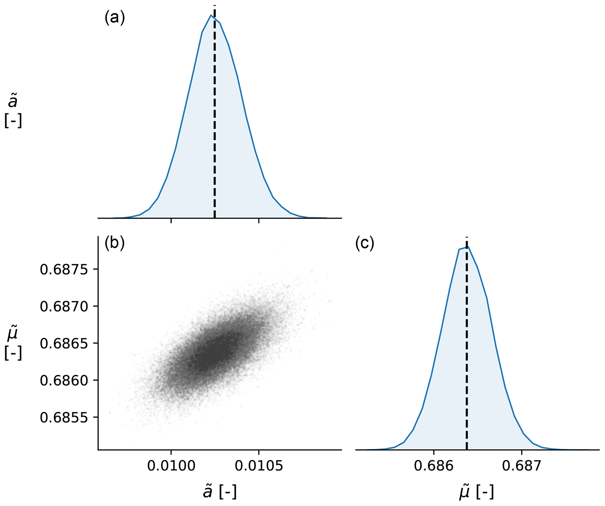
Figure 3Panel (b) of the posterior distributions of the inverted parameters and (marginalised over the nuisance parameter ν2) for the laboratory injection experiment. Panels (a) and (c) show the posterior probability density distribution of each parameter, whereas (b) shows the co-variance of posterior samples. The black dashed lines in the distribution plots (a, c) indicate the median value.
We continue by fitting the (logarithm of) measured slip rate based on Eq. (3), using the parameter values inferred in the previous step to compute the time evolution of tan ψ. Without loss of generality, we define µm s−1 L−1, so that represents the grain boundary friction coefficient at a slip rate of . Since ϕ0 and ϕc individually are ambiguous, we take ϕ0=0.25 and increment this value by the inverted ϕc−ϕ0 to obtain ϕc=0.34. The slip rate parameters are extremely well resolved (see Fig. 3), and found to be and , with minimal trade-off between the two parameters. With these parameters, the fit to the slip rate data is excellent (Fig. 4b).
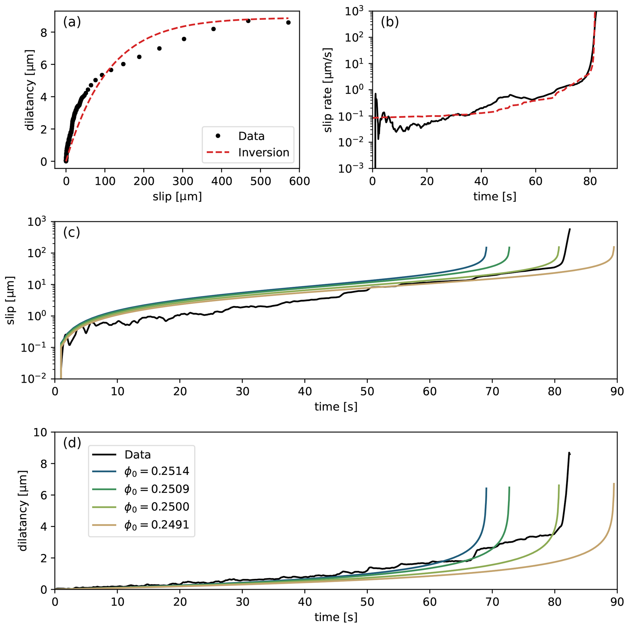
Figure 4Results of the inversion procedure. (a) Dilatancy versus slip, with the inversion curve given by Eq. (6); (b) slip rate versus time, with the inversion curve given by Eq. (1a); (c, d) forward model results of slip and dilatancy for a (narrow) range of initial porosity ϕ0 (as indicated in the legend). The reference value of ϕ0 is obtained from the inversion of Eq. (6).
Finally, for verification, we numerically solve the forward model given by Eqs. (1a) and (1b) with the parameters obtained in the inversion procedure (Fig. 4c and d). While we obtain an excellent fit with the observed time evolution of slip and dilatancy, we also find that the forward model is extremely sensitive to the initial condition ϕ0. While the overall features of the simulated sample response are similar, the exponential sensitivity to porosity leads to critical behaviour and strong variations in the timing of the sample failure. Since the rate of increase in porosity is proportional to the shear strain rate, which in turn is an exponential function of porosity (refer to Eqs. 1b and 3), the positive feedback loop leads to an extremely rapidly diverging state. This is highlighted in Fig. 4c and d, where we vary the initial porosity between 0.2491 and 0.2514 (−1.5 % and +1 % around the reference value of 0.25). The initial condition that gives the best match in terms of the onset of accelerated slip is close to the initially chosen value of ϕ0=0.25, although we assign no significance to tiny deviations in the initial porosity. In a laboratory setting, the sensitivity of the modelled slip rate falls well within the measurement resolution of the sample porosity (typically of the order of several percent of units of porosity), so verification of this sensitivity would be challenging.
3.2 Field experiment
Encouraged by the results of the proposed inversion method for the laboratory experiment, we continue to apply the same procedure to the field injection test of Cappa et al. (2019). Like in the laboratory experiment, the in situ pressurisation of a tectonic fault triggered accelerating slip and, associated with it, fault opening (dilatancy) – see Fig. 5a. While the acceleration of shear and normal displacement on the fault was more gradual than in the laboratory experiment, a phase of rapidly accelerating slip at t>800 s can be clearly seen. The amount of dilatancy measured as a function of slip (Fig. 5b) was proportionally more than in the laboratory experiment by at least 1 order of magnitude, so we expect a priori that the frictional parameters inferred from the laboratory cannot immediately describe the behaviour of the fault in situ. Indeed, when we perform the inversion of the dilatancy-slip data from the field experiment, we find median values of , , and (Fig. 6).
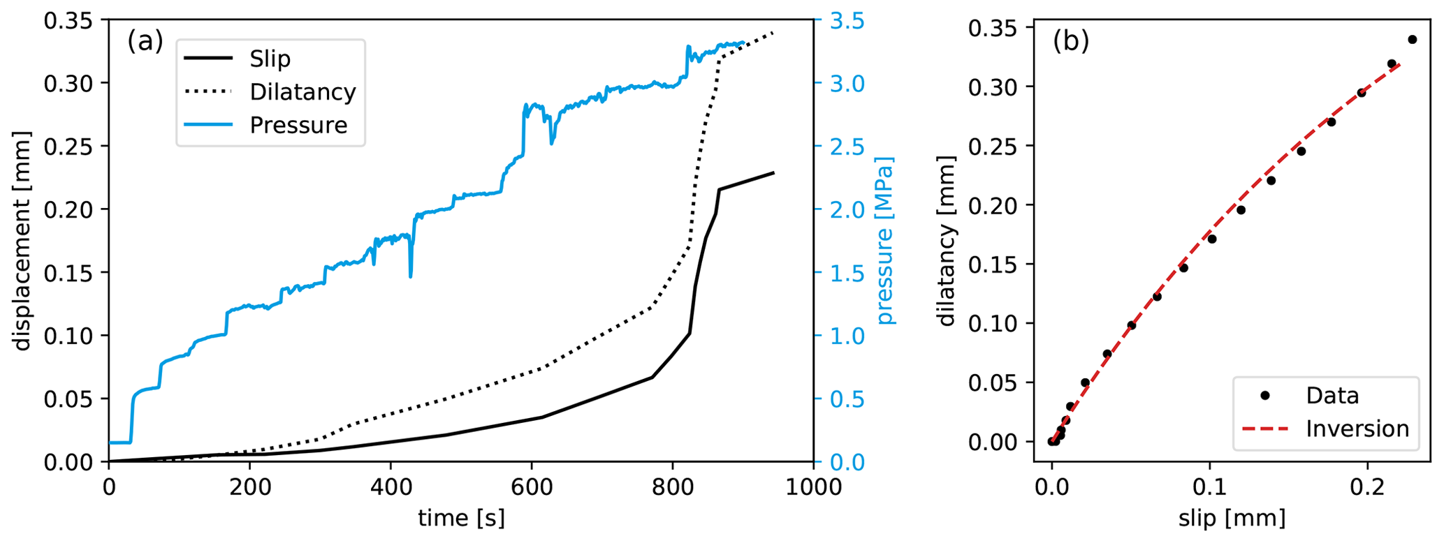
Figure 5(a) Measurements of fault shear and normal displacement and fluid pressure during the field injection test of Cappa et al. (2019); (b) inversion of the dilatancy measured during the field injection experiment. To produce a reasonable fit to the data, an unrealistically high value of the dilatancy parameter H=6.4 was required.
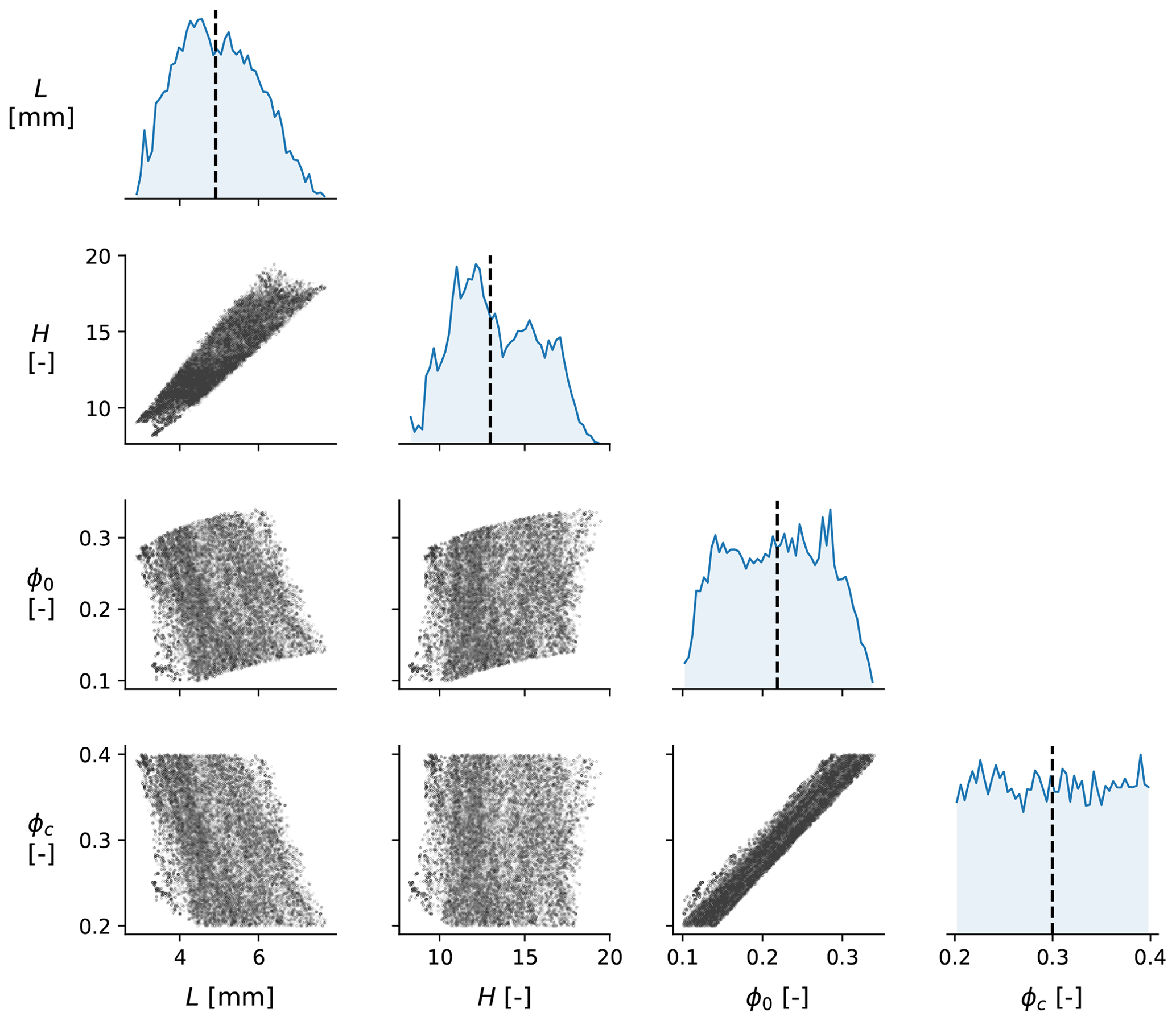
Figure 6Corner plot of the posterior distributions of the inverted parameters L, H, ϕ0, and ϕc (marginalised over the nuisance parameter ν2) for the field injection experiment. The main diagonal panels show the posterior probability density distribution of each parameter, whereas the off-diagonal panels show the co-variance of posterior samples.
While these other values seem entirely reasonable, the inferred value of H is well above the estimated upper bound of . This suggests that the CNS model is unable to explain the relationship between fault slip and fault opening in this experiment. In the CNS model, dilatancy is envisioned to originate from grain sliding and rolling, neighbour swapping, and “jostling”, which requires a volume increase of the gouge to accommodate. However, the model fault itself is mathematically planar, and so no dilatancy occurs due to geometric constraints. In the case of a macroscopically non-planar fault geometry (as is inevitable for tectonic faults; Candela et al., 2012), additional dilatancy (with associated permeability changes) at the onset of slip is necessary. Moreover, poro-elastic effects (elastic fault opening) due to fluid pressure changes are not considered here. The inability of the CNS model to describe the fault opening with a reasonable choice of parameters is therefore not a shortcoming of the CNS model (which describes the mechanics of a small representative volume element), but is rather due to an incomplete coupling with processes that transcend the scale envisioned by the CNS model. For simple, spatially uniform relationships between geometric fault opening and fault slip, this first-order contribution to the fault dilatation may be incorporated into Eq. (1b). However, for more realistic (i.e. spatially heterogeneous) fault opening, a multi-scale numerical extension of the adopted model is required.
Since the CNS model fault strength (and therefore the fault slip rate) is directly controlled by the dilatancy parameter H, it is unwarranted to attempt to infer and based on the parameters inferred from the dilatancy. While this may seem like a severe limitation of the CNS model, it actually serves as an important indication of the applicability of the model, and the validity of its parameters, when attempting to extrapolate to nature. Moreover, the basic mechanics of the CNS model are still expected to govern the strength and slip rate of the fault, even though part of the model predictions (the dilatancy) cannot be constrained by independent measurements. By numerically solving the forward model, the fault slip as a function of time and fluid pressure may be reproduced within a reasonable range of parameter values, for which the predicted fault opening would likely be much less than measured by Cappa et al. (2019).
4.1 Comparison with rate-and-state friction
Traditionally, laboratory experiments are interpreted within the framework of rate-and-state friction (RSF), commonly presented as (Dieterich, 1979; Ruina, 1983)
where μ(V,θ) is the macroscopic friction coefficient at slip rate V and “state” θ, μ* is a reference friction coefficient at slip rate V*, and a, b, and Dc are empirical constants. As has been shown by Chen et al. (2017), the CNS model is asymptotically identical to RSF for small departures from steady state, for which the CNS equivalents of the RSF parameters a, b, and Dc can be treated as constants. For large departures from steady state, the behaviours predicted by CNS and RSF diverge, as the aforementioned parameters can no longer be considered to be constant (van den Ende et al., 2018). Nonetheless, because of their similarity, the limitations of the CNS model also apply to rate-and-state friction. One advantage of using the CNS microphysical model over traditional RSF, is that the governing parameters have a more physically meaningful interpretation. Even though numerous studies have attempted to elucidate the physical origin of RSF (Aharonov and Scholz, 2018; Brechet and Estrin, 1994; Ikari et al., 2016; Putelat et al., 2011), in practice these theoretical constraints are not considered. Instead, it is more convenient to constrain the RSF parameters empirically through laboratory velocity-step experiments (Blanpied et al., 1998; Carpenter et al., 2016; Chester, 1994; Hunfeld et al., 2017; Reinen and Weeks, 1993). With these laboratory measurements of the RSF parameters, fault slip observed during decametric-scale fluid injection tests can be accurately modelled (Cappa et al., 2019), although the same behaviour can be obtained for a wide range of parameter values: in the study of Cappa et al. (2019) a similar fit to the data was obtained for velocity-weakening () and velocity-strengthening () friction, even though seismic slip can only be produced in the former case of velocity-weakening friction. Hence, more observational constraints are required to distinguish between the different types of behaviour.
Aside from the fault-parallel slip, the fault opening potentially provides a second prominent constraint. In the classical RSF framework, volumetric deformation is not explicitly accounted for. Traditionally, the state parameter θ has been interpreted as encoding the average lifetime of asperity contacts (at steady state) or the relative area of asperity contacts (Dieterich, 1994; Scholz, 2019), both of which do not entail volumetric deformation of the fault gouge. Empirical relations between the state parameter θ and porosity have also been proposed (Segall and Rice, 1995; Sleep, 2005) and used in hydro-mechanical modelling (Jeanne et al., 2018), but these relations are typically not employed as additional constraints of the RSF constitutive parameters. Moreover, relations between the steady-state coefficient of friction (and its velocity dependence) have been established based on energy balance considerations (Beeler et al., 1996; Marone et al., 1990). Since these relations pertain to the steady-state coefficient of friction, they do not apply to non-steady-state conditions (for which and ) and do not offer additional insight on the relationship between θ and ϕ. On the other hand, volumetric deformation is an integral part of the CNS model, hence allowing (and requiring) us to incorporate these measurements to arrive at a better constrained set of parameters.
4.2 Relationships between experiments and nature
While the CNS microphysical parameters can be directly estimated from laboratory experiments, their incorporation into numerical models of tectonic faults may be subject to moderation based on geological or physical considerations. In laboratory experiments conducted at room ambient conditions and comparatively high deformation rates (of the order of micrometres per second up to millimetres per second), the gouge porosity remains close to the critical-state porosity. Likewise, in the laboratory experiment of Cappa et al. (2019), the initial porosity was estimated to be less than 0.1 units of porosity below the critical-state porosity. Given longer timescales and higher temperatures, compaction induced by one or more time-dependent creep mechanisms (such as pressure solution creep or subcritical crack growth) would gradually reduce the porosity of the gouge, thereby increasing its strength and critical fluid pressure at which the fault slip rates become appreciable. In numerical simulations of fault slip, the initial state of a tectonic fault is likely not the same as for the laboratory fault. Fortunately, this initial state could be estimated from microstructural analyses of drill cores. Moreover, the choice of the initial state of the fault does not affect any of the other frictional parameters of the CNS model. This is in contrast to rate-and-state friction, where the initial value of the state parameter (θ at t=0) should also affect the magnitude of b, which has been found to increase with decreasing porosity (or increasing θ; Chen et al., 2015, 2017).
The property that b (or more precisely: b∕Dc) is sensitive to the gouge porosity can also be derived from stability analysis of the CNS model. Consider the general criterion for unstable slip of a spring block:
where K is the shear stiffness of the fault. For an instantaneous step change in velocity, for t>0. Assuming that unstable slip is governed by the onset of granular flow, the shear strength is given by the CNS model as (Chen and Spiers, 2016)
Hence, using Eq. (1b), the stability criterion can be expressed in terms of microstructural quantities as (van den Ende et al., 2018)
In the vicinity of steady state, the above statement should be identical to the stability criterion derived from rate-and-state friction, i.e. (Rubin and Ampuero, 2005)
Here, Kb is a critical stiffness value that facilitates acceleration of slip (seismic or aseismic). From the comparison of the two inequalities, it can be concluded that the Kb therefore must increase with decreasing porosity. This was also observed in the discrete element model simulations of van den Ende and Niemeijer (2018), which were conducted completely independently of the assumptions and limitations of the CNS model. We note that the comparison between Eqs. (10) and (11) only holds in the vicinity of steady state. Nonetheless, Eq. (10) can be used to describe the stability of fault slip far from steady state, circumventing the issue of the velocity and state dependence of a, b, and Dc (as observed by Cappa et al., 2019; den Hartog and Spiers, 2013; Reinen et al., 1992; Takahashi et al., 2017, and many others). For a more detailed analysis of the frictional stability of a model fault governed by the CNS model, we refer to Chen and Niemeijer (2017).
Combining now the observations made in Sect. 3 with the discussion above, we propose that the seismogenic potential of faults subjected to fluid pressure perturbations is best described in terms of the dilatant behaviour of the fault and its initial degree of compaction. One can infer the microphysical parameters H, ϕc, , and from laboratory experiments, and assume reasonable in situ values of ϕ and L for the tectonic fault to simulate its response to a changing stress field (fluid pressure). If permitted by the numerical method, fault non-planarity, permeability changes, and elastic moduli reduction may be introduced to add further complexity, as anticipated based on the results of Sect. 3.2. In this way, the evident pressure and velocity dependence of the rate-and-state friction parameters can directly be accounted for in a self-consistent and transparent manner and the model outcomes interpreted in terms of physical observables.
In this work, we analysed the fluid injection experiments conducted by Cappa et al. (2019) in the laboratory and in situ, in terms of the Chen–Niemeijer–Spiers (CNS) microphysical model. We proposed a Bayesian inversion approach to extract the governing parameters without the need for numerically solving the forward problem, while elucidating the uncertainties and trade-offs between the model parameters. We showed that while the localised gouge layer thickness L and the dilatancy parameter H can be well resolved, the initial and critical-state porosities trade off perfectly, so that only their difference ϕc−ϕ0 can be resolved in the experiments. When numerically solving the forward model with the inferred parameter values, we obtained almost perfect agreement with the measurements, indicating that the CNS model accurately describes fault deformation in response to a fluid pressure perturbation. When the same inversion approach was applied to a decametric-scale field injection experiment, we found that the inferred parameters fell outside of the feasible range of values, highlighting the relevance of other mechanisms, such as fault structure and poro-elastic effects, in this scenario.
The excellent agreement between the CNS model and the laboratory data allows us to interpret the dynamics of the fault in terms of volumetric deformation (porosity changes). By doing so, we circumvent the velocity dependence of the rate-and-state friction parameters a, b, and Dc, which increases the predictive power of numerical models of natural faults. Adopting the CNS model expedites the extrapolation of laboratory results to nature and permits better assessment of the applicability of the model and accuracy of the parameter values.
A Python script that reproduces the results and figures in this paper, along with the laboratory and field injection data, is available at https://doi.org/10.6084/m9.figshare.12613007 (van den Ende et al., 2020).
MPAvdE conceptualised the study and performed the analyses. MMS and FC provided the laboratory and field data. JPA supervised MPAvdE. All authors discussed and prepared the contents of the paper.
The authors declare that they have no conflict of interest.
This article is part of the special issue “Thermo–hydro–mechanical–chemical (THMC) processes in natural and induced seismicity”. It is a result of the 7th International Conference on Coupled THMC Processes, Utrecht, Netherlands, 3–5 July 2019.
The authors thank the topical editor André Niemeijer and two anonymous reviewers for their encouraging and constructive comments on the paper. Martijn P. A. van den Ende, Frédéric Cappa, and Jean-Paul Ampuero are supported by French government through the UCAJEDI Investments in the Future project managed by the National Research Agency (ANR) with the reference number ANR-15-IDEX-01.
This research has been supported by the Agence Nationale de la Recherche (grant no. ANR-15-IDEX-01).
This paper was edited by André R. Niemeijer and reviewed by two anonymous referees.
Aharonov, E. and Scholz, C. H.: A Physics-Based Rock Friction Constitutive Law: Steady State Friction, J. Geophys. Res.-Sol. Ea., 123, 1591–1614, https://doi.org/10.1002/2016JB013829, 2018. a
Beeler, N. M., Tullis, T. E., Blanpied, M. L., and Weeks, J. D.: Frictional Behavior of Large Displacement Experimental Faults, J. Geophys. Res.-Sol. Ea., 101, 8697–8715, https://doi.org/10.1029/96JB00411, 1996. a
Blanpied, M. L., Marone, C. J., Lockner, D. A., Byerlee, J. D., and King, D. P.: Quantitative Measure of the Variation in Fault Rheology Due to Fluid-Rock Interactions, J. Geophys. Res.-Sol. Ea., 103, 9691–9712, https://doi.org/10.1029/98JB00162, 1998. a, b
Boulton, C., Niemeijer, A. R., Hollis, C. J., Townend, J., Raven, M. D., Kulhanek, D. K., and Shepherd, C. L.: Temperature-Dependent Frictional Properties of Heterogeneous Hikurangi Subduction Zone Input Sediments, ODP Site 1124, Tectonophysics, 757, 123–139, https://doi.org/10.1016/j.tecto.2019.02.006, 2019. a
Brechet, Y. and Estrin, Y.: The Effect of Strain Rate Sensitivity on Dynamic Friction of Metals, Scr. Metall. Mater., 30, 1449–1454, https://doi.org/10.1016/0956-716X(94)90244-5, 1994. a
Candela, T., Renard, F., Klinger, Y., Mair, K., Schmittbuhl, J., and Brodsky, E. E.: Roughness of Fault Surfaces over Nine Decades of Length Scales, J. Geophys. Res.-Sol. Ea., 117, B08409, https://doi.org/10.1029/2011JB009041, 2012. a
Cappa, F., Scuderi, M. M., Collettini, C., Guglielmi, Y., and Avouac, J.-P.: Stabilization of Fault Slip by Fluid Injection in the Laboratory and in Situ, Sci. Adv., 5, eaau4065, https://doi.org/10.1126/sciadv.aau4065, 2019. a, b, c, d, e, f, g, h, i, j, k, l, m, n, o, p
Carpenter, B., Collettini, C., Viti, C., and Cavallo, A.: The Influence of Normal Stress and Sliding Velocity on the Frictional Behaviour of Calcite at Room Temperature: Insights from Laboratory Experiments and Microstructural Observations, Geophys. J. Int., 205, 548–561, https://doi.org/10.1093/gji/ggw038, 2016. a
Catalli, F., Rinaldi, A. P., Gischig, V., Nespoli, M., and Wiemer, S.: The Importance of Earthquake Interactions for Injection-Induced Seismicity: Retrospective Modeling of the Basel Enhanced Geothermal System, Geophys. Res. Lett., 43, 4992–4999, https://doi.org/10.1002/2016GL068932, 2016. a
Chen, J. and Niemeijer, A. R.: Seismogenic Potential of a Gouge-Filled Fault and the Criterion for Its Slip Stability: Constraints From a Microphysical Model, J. Geophys. Res.-Sol. Ea., 122, 9658–9688, https://doi.org/10.1002/2017JB014228, 2017. a
Chen, J. and Spiers, C. J.: Rate and State Frictional and Healing Behavior of Carbonate Fault Gouge Explained Using Microphysical Model, J. Geophys. Res.-Sol. Ea., 121, 8642–8665, https://doi.org/10.1002/2016JB013470, 2016. a, b, c, d, e, f
Chen, J., Verberne, B. A., and Spiers, C. J.: Effects of Healing on the Seismogenic Potential of Carbonate Fault Rocks: Experiments on Samples from the Longmenshan Fault, Sichuan, China, J. Geophys. Res.-Sol. Ea., 120, 5479–5506, https://doi.org/10.1002/2015JB012051, 2015. a
Chen, J., Niemeijer, A. R., and Spiers, C. J.: Microphysically Derived Expressions for Rate-and-State Friction Parameters, a, b, and Dc, J. Geophys. Res.-Sol. Ea., 122, 9627–9657, https://doi.org/10.1002/2017JB014226, 2017. a, b
Chester, F. M.: Effects of Temperature on Friction: Constitutive Equations and Experiments with Quartz Gouge, J. Geophys. Res., 99, 7247, https://doi.org/10.1029/93JB03110, 1994. a, b
Cubas, N., Lapusta, N., Avouac, J.-P., and Perfettini, H.: Numerical Modeling of Long-Term Earthquake Sequences on the NE Japan Megathrust: Comparison with Observations and Implications for Fault Friction, Earth Planet. Sc. Lett., 419, 187–198, https://doi.org/10.1016/j.epsl.2015.03.002, 2015. a
Dempsey, D. and Riffault, J.: Response of Induced Seismicity to Injection Rate Reduction: Models of Delay, Decay, Quiescence, Recovery, and Oklahoma, Water Resour. Res., 55, 656–681, https://doi.org/10.1029/2018WR023587, 2019. a
den Hartog, S. and Spiers, C.: Influence of Subduction Zone Conditions and Gouge Composition on Frictional Slip Stability of Megathrust Faults, Tectonophysics, 600, 75–90, https://doi.org/10.1016/j.tecto.2012.11.006, 2013. a
Derode, B., Guglielmi, Y., Barros, L. D., and Cappa, F.: Seismic Responses to Fluid Pressure Perturbations in a Slipping Fault, Geophys. Res. Lett., 42, 3197–3203, https://doi.org/10.1002/2015GL063671, 2015. a
Dieterich, J.: A Constitutive Law for Rate of Earthquake Production and Its Application to Earthquake Clustering, J. Geophys. Res.-Sol. Ea., 99, 2601–2618, https://doi.org/10.1029/93JB02581, 1994. a
Dieterich, J. H.: Modeling of Rock Friction: 1. Experimental Results and Constitutive Equations, J. Geophys. Res., 84, 2161, https://doi.org/10.1029/JB084iB05p02161, 1979. a, b
Duboeuf, L., De Barros, L., Cappa, F., Guglielmi, Y., Deschamps, A., and Seguy, S.: Aseismic Motions Drive a Sparse Seismicity During Fluid Injections Into a Fractured Zone in a Carbonate Reservoir: Injection-Induced (A)Seismic Motions, J. Geophys. Res.-Sol. Ea., 122, 8285–8304, https://doi.org/10.1002/2017JB014535, 2017. a, b
Ellsworth, W. L.: Injection-Induced Earthquakes, Science, 341, 1225942, https://doi.org/10.1126/science.1225942, 2013. a
Elsworth, D., Spiers, C. J., and Niemeijer, A. R.: Understanding Induced Seismicity, Science, 354, 1380–1381, https://doi.org/10.1126/science.aal2584, 2016. a
Foreman-Mackey, D., Hogg, D. W., Lang, D., and Goodman, J.: Emcee: The MCMC Hammer, Publ. Astron. Soc. Pacific, 125, 306–312, https://doi.org/10.1086/670067, 2013. a
Frye, K. M. and Marone, C.: The Effect of Particle Dimensionality on Granular Friction in Laboratory Shear Zones, Geophys. Res. Lett., 29, 22-1–22-4, https://doi.org/10.1029/2002GL015709, 2002. a
Goebel, T. H. W. and Brodsky, E. E.: The Spatial Footprint of Injection Wells in a Global Compilation of Induced Earthquake Sequences, Science, 361, 899–904, https://doi.org/10.1126/science.aat5449, 2018. a
Guglielmi, Y., Cappa, F., Avouac, J.-P., Henry, P., and Elsworth, D.: Seismicity Triggered by Fluid Injection–Induced Aseismic Slip, Science, 348, 1224–1226, https://doi.org/10.1126/science.aab0476, 2015. a
Hazzard, J. F. and Mair, K.: The Importance of the Third Dimension in Granular Shear, Geophys. Res. Lett., 30, 1708, https://doi.org/10.1029/2003GL017534, 2003. a
He, C., Tan, W., and Zhang, L.: Comparing Dry and Wet Friction of Plagioclase: Implication to the Mechanism of Frictional Evolution Effect at Hydrothermal Conditions, J. Geophys. Res.-Sol. Ea., 121, 6365–6383, https://doi.org/10.1002/2016JB012834, 2016. a
Hunfeld, L. B., Niemeijer, A. R., and Spiers, C. J.: Frictional Properties of Simulated Fault Gouges from the Seismogenic Groningen Gas Field Under In Situ P-T-Chemical Conditions, J. Geophys. Res.-Sol. Ea., 122, 8969–8989, https://doi.org/10.1002/2017JB014876, 2017. a, b
Ikari, M. J., Carpenter, B. M., and Marone, C.: A Microphysical Interpretation of Rate- and State-Dependent Friction for Fault Gouge, Geochem. Geophy. Geosy. 17, 1660–1677, https://doi.org/10.1002/2016GC006286, 2016. a
Jeanne, P., Guglielmi, Y., Rutqvist, J., Nussbaum, C., and Birkholzer, J.: Permeability Variations Associated With Fault Reactivation in a Claystone Formation Investigated by Field Experiments and Numerical Simulations, J. Geophys. Res.-Sol. Ea., 123, 1694–1710, https://doi.org/10.1002/2017JB015149, 2018. a
Kaproth, B. M., Kacewicz, M., Muhuri, S., and Marone, C.: Permeability and Frictional Properties of Halite-Clay-Quartz Faults in Marine-Sediment: The Role of Compaction and Shear, Mar. Petrol. Geol., 78, 222–235, https://doi.org/10.1016/j.marpetgeo.2016.09.011, 2016. a
Kroll, K. A., Richards-Dinger, K. B., and Dieterich, J. H.: Sensitivity of Induced Seismic Sequences to Rate-and-State Frictional Processes, J. Geophys. Res.-Sol. Ea., 122, 10207–10219, https://doi.org/10.1002/2017JB014841, 2017. a
Marone, C., Raleigh, C. B., and Scholz, C. H.: Frictional Behavior and Constitutive Modeling of Simulated Fault Gouge, J. Geophys. Res., 95, 7007, https://doi.org/10.1029/JB095iB05p07007, 1990. a
McClure, M. W. and Horne, R. N.: Investigation of Injection-Induced Seismicity Using a Coupled Fluid Flow and Rate/State Friction Model, Geophysics, 76, WC181–WC198, https://doi.org/10.1190/geo2011-0064.1, 2011. a
Niemeijer, A. R. and Spiers, C. J.: A Microphysical Model for Strong Velocity Weakening in Phyllosilicate-Bearing Fault Gouges, J. Geophys. Res., 112, B10405, https://doi.org/10.1029/2007JB005008, 2007. a, b, c, d, e, f
Noda, H., Sawai, M., and Shibazaki, B.: Earthquake Sequence Simulations with Measured Properties for JFAST Core Samples, Philos. Trans. Roy. Soc. A-Math., 375, 20160003, https://doi.org/10.1098/rsta.2016.0003, 2017. a
Putelat, T., Dawes, J. H., and Willis, J. R.: On the Microphysical Foundations of Rate-and-State Friction, J. Mech. Phys. Solid., 59, 1062–1075, https://doi.org/10.1016/j.jmps.2011.02.002, 2011. a
Reinen, L. A. and Weeks, J. D.: Determination of Rock Friction Constitutive Parameters Using an Iterative Least Squares Inversion Method, J. Geophys. Res., 98, 15937, https://doi.org/10.1029/93JB00780, 1993. a
Reinen, L. A., Tullis, T. E., and Weeks, J. D.: Two-Mechanism Model for Frictional Sliding of Serpentinite, Geophys. Res. Lett., 19, 1535–1538, https://doi.org/10.1029/92GL01388, 1992. a
Rivet, D., Barros, L. D., Guglielmi, Y., Cappa, F., Castilla, R., and Henry, P.: Seismic Velocity Changes Associated with Aseismic Deformations of a Fault Stimulated by Fluid Injection, Geophys. Res. Lett., 43, 9563–9572, https://doi.org/10.1002/2016GL070410, 2016. a
Rubin, A. M. and Ampuero, J.-P.: Earthquake Nucleation on (Aging) Rate and State Faults, J. Geophys. Res.-Sol. Ea., 110, B11312, https://doi.org/10.1029/2005JB003686, 2005. a
Ruina, A.: Slip Instability and State Variable Friction Laws, J. Geophys. Res.-Sol. Ea., 88, 10359–10370, https://doi.org/10.1029/JB088iB12p10359, 1983. a, b
Rutqvist, J., Birkholzer, J., Cappa, F., and Tsang, C. F.: Estimating Maximum Sustainable Injection Pressure during Geological Sequestration of CO2 Using Coupled Fluid Flow and Geomechanical Fault-Slip Analysis, Energ. Convers. Manage., 48, 1798–1807, https://doi.org/10.1016/j.enconman.2007.01.021, 2007. a
Sawai, M., Niemeijer, A. R., Plümper, O., Hirose, T., and Spiers, C. J.: Nucleation of Frictional Instability Caused by Fluid Pressurization in Subducted Blueschist, Geophys. Res. Lett., 43, 2543–2551, https://doi.org/10.1002/2015GL067569, 2016. a
Schoenball, M. and Ellsworth, W. L.: A Systematic Assessment of the Spatiotemporal Evolution of Fault Activation Through Induced Seismicity in Oklahoma and Southern Kansas, J. Geophys. Res.-Sol. Ea., 122, 10189–10206, https://doi.org/10.1002/2017JB014850, 2017. a
Scholz, C. H.: The Mechanics of Earthquakes and Faulting, 3rd Edn., Cambridge University Press, Cambridge, https://doi.org/10.1017/9781316681473, 2019. a
Scuderi, M., Collettini, C., and Marone, C.: Frictional Stability and Earthquake Triggering during Fluid Pressure Stimulation of an Experimental Fault, Earth Planet. Sc. Lett., 477, 84–96, https://doi.org/10.1016/j.epsl.2017.08.009, 2017. a, b
Scuderi, M. M. and Collettini, C.: Fluid Injection and the Mechanics of Frictional Stability of Shale-Bearing Faults, J. Geophys. Res.-Sol. Ea., 123, 8364–8384, https://doi.org/10.1029/2018JB016084, 2018. a
Scuderi, M. M., Marone, C., Tinti, E., Di Stefano, G., and Collettini, C.: Precursory Changes in Seismic Velocity for the Spectrum of Earthquake Failure Modes, Nat. Geosci., 9, 695–700, https://doi.org/10.1038/ngeo2775, 2016. a, b
Segall, P. and Rice, J. R.: Dilatancy, Compaction, and Slip Instability of a Fluid-Infiltrated Fault, J. Geophys. Res.-Sol. Ea., 100, 22155–22171, https://doi.org/10.1029/95JB02403, 1995. a, b
Sleep, N. H.: Physical Basis of Evolution Laws for Rate and State Friction, Geochem. Geophy. Geosy., 6, Q11008, https://doi.org/10.1029/2005GC000991, 2005. a
Takahashi, M., van den Ende, M. P. A., Niemeijer, A. R., and Spiers, C. J.: Shear Localization in a Mature Mylonitic Rock Analog during Fast Slip, Geochem. Geophy. Geosy., 18, 513–530, https://doi.org/10.1002/2016GC006687, 2017. a
Tenthorey, E., Cox, S. F., and Todd, H. F.: Evolution of Strength Recovery and Permeability during Fluid–Rock Reaction in Experimental Fault Zones, Earth Planet. Sc. Lett., 206, 161–172, https://doi.org/10.1016/S0012-821X(02)01082-8, 2003. a
van den Ende, M., Scuderi, M., Cappa, F., and Ampuero, J.-P.: Extracting microphysical fault friction parameters from laboratory-and field injection experiments, figshare, https://doi.org/10.6084/m9.figshare.12613007, 2020. a
van den Ende, M. P. A. and Niemeijer, A. R.: Time-Dependent Compaction as a Mechanism for Regular Stick-Slips, Geophys. Res. Lett., 45, 5959–5967, https://doi.org/10.1029/2018GL078103, 2018. a
van den Ende, M. P. A., Chen, J., Ampuero, J. P., and Niemeijer, A. R.: A Comparison between Rate-and-State Friction and Microphysical Models, Based on Numerical Simulations of Fault Slip, Tectonophysics, 733, 273–295, https://doi.org/10.1016/j.tecto.2017.11.040, 2018. a, b, c, d
Verberne, B. A., van den Ende, M. P. A., Chen, J., Niemeijer, A. R., and Spiers, C. J.: The physics of fault friction: insights from experiments on simulated gouges at low shearing velocities, Solid Earth, 11, 2075–2095, https://doi.org/10.5194/se-11-2075-2020, 2020. a
Wynants-Morel, N., Cappa, F., Barros, L. D., and Ampuero, J.-P.: Stress Perturbation From Aseismic Slip Drives The Seismic Front During Fluid Injection In A Permeable Fault, J. Geophys. Res.-Sol. Ea., 125, e2019JB019179, https://doi.org/10.1029/2019JB019179, 2020. a