Impact of upper mantle convection on lithosphere hyperextension and subsequent horizontally forced subduction initiation

Many plate tectonic processes, such as subduction initiation, are embedded in long-term (>100 Myr) geodynamic cycles often involving subsequent phases of extension, cooling without plate deformation and convergence. However, the impact of upper mantle convection on lithosphere dynamics during such long-term cycles is still poorly understood. We have designed two-dimensional upper-mantle-scale (down to a depth of 660 km) thermo-mechanical numerical models of coupled lithosphere–mantle deformation. We consider visco–elasto–plastic deformation including a combination of diffusion, dislocation and Peierls creep law mechanisms. Mantle densities are calculated from petrological phase diagrams (Perple_X) for a Hawaiian pyrolite. Our models exhibit realistic Rayleigh numbers between 10⁶ and 10⁷, and the model temperature, density and viscosity structures agree with geological and geophysical data and observations. We tested the impact of the viscosity structure in the asthenosphere on upper mantle convection and lithosphere dynamics. We also compare models in which mantle convection is explicitly modelled with models in which convection is parameterized by Nusselt number scaling of the mantle thermal conductivity. Further, we quantified the plate driving forces necessary for subduction initiation in 2D thermo-mechanical models of coupled lithosphere–mantle deformation. Our model generates a 120 Myr long geodynamic cycle of subsequent extension (30 Myr), cooling (70 Myr) and convergence (20 Myr) coupled to upper mantle convection in a single and continuous simulation. Fundamental features such as the formation of hyperextended margins, upper mantle convective flow and subduction initiation are captured by the simulations presented here. Compared to a strong asthenosphere, a weak asthenosphere leads to the following differences: smaller value of plate driving forces necessary for subduction initiation (15 TN m⁻¹ instead of 22 TN m⁻¹) and locally larger suction forces. The latter assists in establishing single-slab subduction rather than double-slab subduction. Subduction initiation is horizontally forced, occurs at the transition from the exhumed mantle to the hyperextended passive margin and is caused by thermal softening. Spontaneous subduction initiation due to negative buoyancy of the 400 km wide, cooled, exhumed mantle is not observed after 100 Myr in model history. Our models indicate that long-term lithosphere dynamics can be strongly impacted by sub-lithosphere dynamics. The first-order processes in the simulated geodynamic cycle are applicable to orogenies that resulted from the opening and closure of embryonic oceans bounded by magma-poor hyperextended rifted margins, which might have been the case for the Alpine orogeny.

1 Introduction

1.1 Convection in the Earth's mantle

In general, the term convection can be used to describe any motion of a fluid driven by external or internal forces (Ricard et al., 1989). Prout (1834) derived this term from the Latin word “convectio” (to carry or to convey) to distinguish between advection-dominated heat transfer and conduction- and radiation-dominated heat transfer.

On Earth, heat transfer through the lithosphere is dominated by thermal conduction, while heat transfer through the underlying mantle is dominated by advection of material (e.g. Turcotte and Schubert, 2014). Convection may involve either the whole mantle, down to the core–mantle boundary, or only specific mantle layers. At temperature and pressure conditions corresponding to a depth of about 660 km, the mineralogy of peridotite changes from γ-spinel to perovskite + magnesiowüstite. This phase transition is endothermic, which means it has a negative pressure–temperature, the so-called Clapeyron slope. Therefore, the penetration of cold slabs subducting into the lower mantle and hot plumes rising into the upper mantle may be delayed (Schubert et al., 2001). The 660 km phase transition can therefore represent a natural boundary that separates two convecting layers. Laboratory experiments, tomographic images and calculations on the Earth's heat budget deliver evidence that a mixed mode of both types best explains convection in the present-day Earth's mantle (Li et al., 2008; Chen, 2016).

Any convecting system can be described by a dimensionless number, the so-called Rayleigh number. It is defined as the ratio of the diffusive and the advective timescale of heat transfer (see also Eq. B1). The critical value of the Rayleigh number necessary for the onset of convection in the Earth's mantle is typically of the order of 1000 (Schubert et al., 2001). Convection in the Earth's mantle can occur at Rayleigh numbers in the range of 10⁶–10⁹ depending on the heating mode of the system and whether convection is layered or includes the whole mantle (Schubert et al., 2001). The higher the Rayleigh number, the more vigorous the convection; i.e. advection of material occurs at a higher speed. The vigour of both whole and layered mantle convection is inter alia controlled by the mantle density, the temperature gradient across and the effective viscosity of the mantle. However, unlike the density and thermal structures, the viscosity structure of the mantle is subject to large uncertainty. Viscosity is not a direct observable and can only be inferred by inverting observable geophysical data such as data for glacial isostatic adjustment (e.g. Mitrovica and Forte, 2004) or seismic anisotropy data (e.g. Behn et al., 2004). Especially at depths of ca. 100–300 km, in the so-called asthenosphere, the inferred value for viscosity varies greatly (see Fig. 2 in Forte et al., 2010). Values for effective viscosity in this region can be up to 2 orders of magnitude lower than estimates for the average upper mantle viscosity of ≈10²¹ Pa s (Hirth and Kohlstedt, 2003; Becker, 2017).

1.2 Long-term geodynamic cycle and coupled lithosphere–mantle deformation

Many coupled lithosphere–mantle deformation processes, such as the formation of hyperextended passive margins and the mechanisms leading to the initiation of subduction (e.g. Peron-Pinvidic et al., 2019; Stern and Gerya, 2018), are still elusive. Crameri et al. (2020) compiled a database from recent subduction zones to investigate whether subduction initiation was vertically (spontaneous) or horizontally forced (induced; see also Stern, 2004, for terminology). They concluded that, during the last ca. 100 Myr, the majority of subduction initiation events were likely horizontally forced. Recent numerical studies have investigated thermal softening as a feasible mechanism for horizontally forced subduction initiation (Thielmann and Kaus, 2012; Jaquet and Schmalholz, 2018; Kiss et al., 2020). In these models, horizontally forced subduction was initiated without prescribing a major weak zone cross-cutting through the lithosphere. These models do not require further assumptions on other softening mechanisms, such as microscale grain growth or fluid- and reaction-induced softening. Therefore, these models are likely the simplest to study horizontally forced subduction initiation.

Geodynamic processes, such as lithosphere extension or convergence, are frequently studied separately. In fact, many studies show that these processes are embedded in longer-term cycles, such as the Wilson cycle (Wilson, 1966; Wilson et al., 2019). Over large timescales ($>\approx \mathrm{80}$ Myr), tectonic inheritance of earlier extension and cooling events (Chenin et al., 2019) together with mantle convection (Solomatov, 2004) presumably had a major impact on subsequent convergence and subduction. Certainly, subduction initiation at passive margins during convergence can be studied without a previous extension and cooling stage (e.g. Kiss et al., 2020). An initial passive margin geometry and thermal field must then be constructed ad hoc for the model configuration. However, it is then uncertain whether the applied model would have generated a stable margin geometry and its characteristic thermal structure during an extension simulation. In other words, it is unclear whether the initial margin configuration is consistent with the applied model.

Plenty of numerical studies modelling the deformation of the lithosphere and the underlying mantle do not directly model convective flow below the lithosphere (e.g. Jaquet and Schmalholz, 2018; Gülcher et al., 2019; Beaussier et al., 2019; Erdös et al., 2019; Li et al., 2019). Ignoring convection below the lithosphere in numerical simulations is unlikely to be problematic if the duration of the simulated deformation does not exceed a few tens of millions of years. In such short time intervals, the diffusive cooling of the lithosphere is likely negligible. However, convection in the Earth's mantle regulates the long-term thermal structure of the lithosphere (Richter, 1973; Parsons and McKenzie, 1978) and therefore has a fundamental control on the lithospheric strength. Furthermore, mantle flow can exert suction forces on the lithosphere (e.g. Conrad and Lithgow-Bertelloni, 2002). Numerical studies show that these suction forces can assist in the initiation of subduction (Baes et al., 2018). Therefore, coupling mantle convection to lithospheric-scale deformation can potentially improve our understanding of processes acting on long-term geodynamic cycles of the lithosphere.

Here, we present two-dimensional (2D) thermo-mechanical numerical simulations modelling the long-term cycle of coupled lithosphere–mantle deformation. The modelled geodynamic cycle comprises a 120 Myr history of extension–cooling–convergence, leading to horizontally forced subduction. We include the mantle down to a depth of 660 km assuming that convection is layered. Timings and deformation velocities for the distinct periods have been chosen to allow for comparison of the model results to the Alpine orogeny. With these models, we investigate and quantify the impact of (1) the viscosity structure of the upper mantle and (2) an effective conductivity parameterization on upper mantle convection and lithospheric deformation. Applying this parameterization diminishes the vigour of convection but maintains a characteristic thermal field for high-Rayleigh-number convection (explained in more detail in the next section and in Appendix B). (3) We also test creep law parameters for wet and dry olivine rheology. Finally, we investigate whether forces induced by upper mantle convection have an impact on horizontally forced subduction initiation.

2 The applied numerical model

The applied numerical algorithm solves the partial differential equations for conservation of mass and momentum coupled to conservation of energy. We consider the deformation of incompressible visco–elasto–plastic slowly flowing fluids under gravity (no inertia). The equations are discretized on a 2D finite-difference staggered grid in the Cartesian coordinate system. Material properties are advected using a marker-in-cell method (Gerya and Yuen, 2003). A fourth-order Runge–Kutta scheme is employed for marker advection and a true free surface is applied (Duretz et al., 2016a). A detailed description of the algorithm is given in Appendix A, and the results of a community convection benchmark test are presented in Appendix C. The applied algorithm has already been used to model processes at different scales, such as deformation of eclogites on the centimetre scale (Yamato et al., 2019), crystal–melt segregation of magma during its ascent in a metre-scale conduit (Yamato et al., 2015), rifting of continental lithosphere (Duretz et al., 2016b; Petri et al., 2019), stress calculations around the Tibetan Plateau (Schmalholz et al., 2019), and within and around the subduction of an oceanic plate (Bessat et al., 2020), as well as modelling Precambrian orogenic processes (Poh et al., 2020). Here, we test the algorithm for the capability of reproducing first-order features of a geodynamic cycle, namely the following: (i) formation of hyperextended magma-poor rifted margins during a 30 Myr extension period applying an absolute extension velocity of 2 cm yr⁻¹p; (ii) separation of the continental crust and opening of a ca. 400 km wide marine basin floored by exhumed mantle material; (iii) generation of upper mantle convection during a 70 Myr cooling period without significant plate deformation; and (iv) subsequent convergence for a period of 20 Myr and horizontally forced subduction initiation in a self-consistent way, which means without modifying the simulation by, for example, adding an ad hoc prominent weak zone across the lithosphere or changing material parameters. During convergence, the self-consistently evolved passive margin system is shortened by applying an absolute convergence velocity of 3 cm yr⁻¹.

2.1 Modelling assumptions and applicability

For simplicity, we consider lithosphere extension that generates magma-poor hyperextended margins and crustal separation, leading to mantle exhumation. This means that we do not need to model melting, lithosphere break-up, mid-ocean ridge formation, and generation of new oceanic crust and lithosphere. Such Wilson-type cycles, involving only embryonic oceans, presumably formed orogens such as the Pyrenees, the western and central Alps, and most of the Variscides of western Europe (e.g. Chenin et al., 2019). Values for deformation periods and rates in the models presented here are chosen to allow for comparison of the model evolution to the Alpine orogeny.

Further, tomographic images from the Mediterranean show large p-wave anomalies in the transition zone (Piromallo and Morelli, 2003), indicating that the 660 km phase transition inhibits the sinking material from penetrating further into the lower mantle. Therefore, we do not include the lower mantle in the model domain and assume that mantle convection is layered.

2.2 Model configuration

The model domain is 1600 km wide and 680 km high, and the applied model resolution is 801×681 grid points (Fig. 1). The minimum z coordinate is set to −660 km, and the top +20 km is left free (no sticky air) to allow for build-up of topography. The top surface (initially at z=0 km) is stress-free. Thus, its position evolves dynamically as topography develops. Mechanical boundary conditions on the remaining boundaries are set to free slip at the bottom and constant material inflow–outflow velocities at the left and right boundary. The boundary velocity is calculated such that the total volume of material flowing through the lateral boundary is conserved. The transition between inflow and outflow occurs at $z=-\mathrm{330}$ km and not at the initially imposed lithosphere–asthenosphere boundary (LAB). Values for deviatoric stresses at this depth are significantly lower compared to those at the base of the lithosphere. This choice avoids boundary effects close to the mechanical lithosphere, and the LAB can develop freely away from the lateral model boundaries. We use the material flow velocity boundary condition rather than bulk extension rates to deform the model units. Applying bulk extension rates and deforming the model domain would change the height of the model domain, which has strong control on the Rayleigh number of the system (Eq. B1). Also, evolution of passive margin geometries becomes dependent on the model width when using bulk extension rates as a mechanical boundary condition (Chenin et al., 2018). It is therefore more practical to use constant velocity boundary conditions with material flow in the type of models presented here.

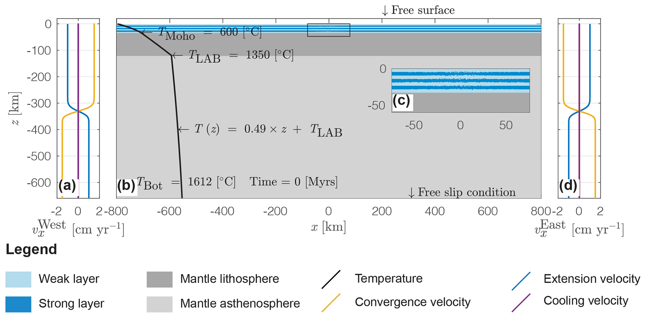
Figure 1 Initial model configuration and boundary conditions. Dark blue represents strong and light blue represents weak crustal units; dark grey represents the mantle lithosphere and light grey the upper mantle. (a) Profile of horizontal velocity for material inflow and outflow along the western model boundary. The blue line indicates the profile for the extension, the purple line indicates the profile for the cooling and the yellow line indicates the profile for the convergence stage. (b) Entire model domain including the material phases (colour code as explained above) and initial vertical temperature profile (black line). (c) Enlargement of the centre of the model domain showing the initial random perturbation on the marker field (see Appendix A) used to localize deformation in the centre of the domain; panel (d) is the same profile as shown in (a) but along the eastern model boundary.

The initial temperature at the surface is set to 15 ^∘C, and temperatures at the crust–mantle (Moho) and at the LAB are 600 and 1350 ^∘C, respectively. Assuming an adiabatic gradient of 0.49 ^∘C km⁻¹ (see Appendix B), the temperature at the model bottom is 1612 ^∘C. Thermal boundary conditions are set to isothermal at the bottom and at the top of the domain, and the left and right boundaries are assumed to be insulating (i.e. no heat flows through lateral boundaries). Model units include a 33 km thick, mechanically layered crust which overlies an 87 km thick mantle lithosphere on top of the upper mantle. The resulting initial thickness of the lithosphere is thus 120 km. The crust includes three mechanically strong and four mechanically weak layers. The thickness of the weak layers is set to 5 km each, and the thickness of the uppermost and lowermost strong layer is set to 4 km, whereas the strong layer in the middle is 5 km thick. This thickness variation allows us to match the total 33 km thickness of the crust without introducing an additional vertical asymmetry. Mechanical layering of the crust was chosen because it is a simple way of considering mechanical heterogeneities in the crust. The layering leads to the formation of numerous structural features observed in natural hyperextended passive margins (Duretz et al., 2016b) without relying on predefined strain softening.

We consider viscous, elastic and brittle–plastic deformation of material in all models presented here. Viscous flow of material is described as a combination of several flow laws. We use dislocation creep for the crustal units and dislocation, diffusion and Peierls creep for mantle units (see also Appendix A). The initial viscosity profile through the upper mantle is calibrated to match viscosity data obtained by Ricard et al. (1989). The applied flow law parameters lie within the error range of the corresponding laboratory flow law estimates (see Table A1).

The difference between mantle lithosphere and upper mantle is temperature only; i.e. all material parameters are the same. The density of the crustal phases is computed with an equation of state (Eq. A3), whereas the density of the mantle phase is pre-computed using Perple_X (Connolly, 2005) for the bulk rock composition of a pyrolite (Workman and Hart, 2005, Fig. A1). A detailed description of the phase transitions and how the initial thermal field is calibrated is given in Appendix B. Surface processes (e.g. erosion and sedimentation) are taken into account through a kinematic approach: if the topography falls below a level of 5 km of depth or rises above 2 km of height, it undergoes either sedimentation or erosion with a constant velocity of 0.5 mm yr⁻¹. In the case of sedimentation, the generated cavity between the old and corrected topographic level is filled with sediments, alternating between calcites and pelites every 2 Myr. This simple parameterization of surface processes moderates the amplitude of topography and may affect geodynamic processes such as subduction.

2.3 Investigated parameters

Among the physical parameters controlling long-term geodynamic evolution (f.e., mantle density, plate velocities), the viscosity structure of the mantle is one of the least constrained. Therefore, we test (1) models with different upper mantle viscosity structures. In model M1, the reference model, the asthenosphere is assumed to be weak with values for viscosity of the order of ≈10¹⁹ Pa s resulting from the applied flow laws. In models M2 and M3 the asthenosphere is assumed to be stronger. Values for viscosities in the asthenosphere are limited by a numerical cut-off value of 1×10²⁰ Pa s in M2 and 5×10²⁰ Pa s in M3. Coupling of lithosphere–mantle deformation is achieved by numerically resolving both lithospheric deformation and upper mantle convection in M1–3. (2) We further test the impact of parameterizing convection on the cycle by scaling the thermal conductivity to the Nusselt number of upper mantle convection (see Appendix B). In these models, we also assume a weak asthenosphere (as in M1) in model M4 and a strong asthenosphere (as in M2) in model M5. The effective conductivity approach has been used, for example, in mantle convection studies for planetary bodies when convection in the mantle is too vigorous to be modelled explicitly (e.g. Zahnle et al., 1988; Tackley et al., 2001; Golabek et al., 2011). Also, it has been used in models of back-arc lithospheric thinning through mantle flow that is induced by subduction of an oceanic plate (e.g. Currie et al., 2008) and in models of lithosphere extension and subsequent compression (e.g. Jammes and Huismans, 2012). (3) We finally investigate the role of the olivine rheology. To this end, we perform an additional model M6 in which the material parameters of the dislocation and diffusion creep mechanism of a dry olivine rheology is replaced by the parameters of a wet olivine rheology (Table A1). In M6, values for all the other parameters, both physical and numerical, are initially equal to those set in M1. Within the error range of values for activation volume and energy of the wet olivine rheology, the viscosity is calibrated to the data obtained by Ricard et al. (1989). However, using the highest possible values for the wet olivine flow law parameters, the maximum viscosity in the upper mantle is initially 1 order of magnitude lower compared to models M1–5. A summary of all simulations is given in Table 1, and all material parameters are summarized in Table A1.

Table 1 Parameters varied in models M1–6.

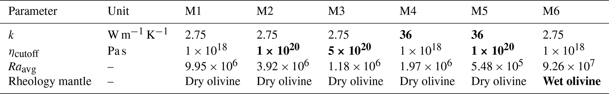
k is thermal conductivity and η_cutoff is the lower viscosity limiter. Ra_avg is the arithmetic average of Rayleigh numbers >1000. Rayleigh numbers are computed locally at each cell centre according to Eq. (B1) after 99 Myr in model history for models M1–5 and after 26 Myr for model M6. Bold font highlights the parameters varied compared to the reference model M1.

3 Results

We first describe the evolution of the reference model M1 and of M6. Model M6 is stopped after the extensional stage because its later evolution is not applicable to present-day Earth. Thereafter, we compare the results of M2–5 to the results of M1 for the individual deformation stages. Finally, we compare the evolution of the plate driving forces in models M1–5 during the entire cycle. The arithmetic average Rayleigh number in all models is significantly larger compared to the critical Rayleigh number Ra_crit=1000. The rifting and cooling periods laterally perturb the thermal field sufficiently to initiate and drive the convection over large timescales in all models presented here.

3.1 Dry olivine rheology: model M1 – reference run

Crustal break-up during the rifting phase in M1 occurs after ca. 8 Myr (Fig. 3a and e). The left continental margin has a length of ca. 200 km and the right margin has a length of ca. 150 km (Fig. 3e). Velocity arrows indicate upward motion of hot material in the centre of the domain (Fig. 3e). Two convection cells begin to establish at this stage below each margin. The viscosity of the upper mantle decreases to minimal values of the order of 10¹⁹ Pa s and increases again up to values of the order of 10²¹ Pa s at the bottom of the model domain (Figs. 3a and 2c). Towards the end of the cooling period (at 97 Myr), M1 has developed circular-shaped convection cells in the upper region of the upper mantle (above $z\approx -\mathrm{400}$ km; Fig. 3b). The average Rayleigh number (see footnote of Table 1) of the system computed at this late stage of the cooling period is ca. 9.95×10⁶, and the size of the cells varies between ca. 50 and ca. 300 km in diameter below the left and right margin, respectively (Fig. 3b). Below the right margin at $z\approx -\mathrm{150}$ km and $x\approx +\mathrm{300}$ km the downward-directed mantle flow of two neighbouring convection cells unifies (Fig. 3f). The top ca. 100 km of the modelled domain remain undeformed; no material is flowing in this region (area without velocity arrows in Fig. 3f). Convergence starts at 100 Myr, and at ca. 102 Myr, a major shear zone forms, breaking the lithosphere below the right margin (inclined zone of reduced effective viscosity in Fig. 3c and g). Velocity arrows in the lithosphere indicate the far-field convergence, whereas velocity arrows in the upper mantle show that convection cells are still active. The exhumed mantle is subducted in one stable subduction zone below the right continental margin. Several convection cells are active in the upper mantle during subduction (see velocity arrows Fig. 3d and h). A trench forms in which sediments are deposited (Fig. 3d and h). Folding of the crustal layers in the overriding plate indicates significant deformation of the crust. The crustal layers of the subducting plate remain relatively undeformed. The viscosity in the asthenosphere remains stable at values of 10¹⁹ Pa s during the entire model history.

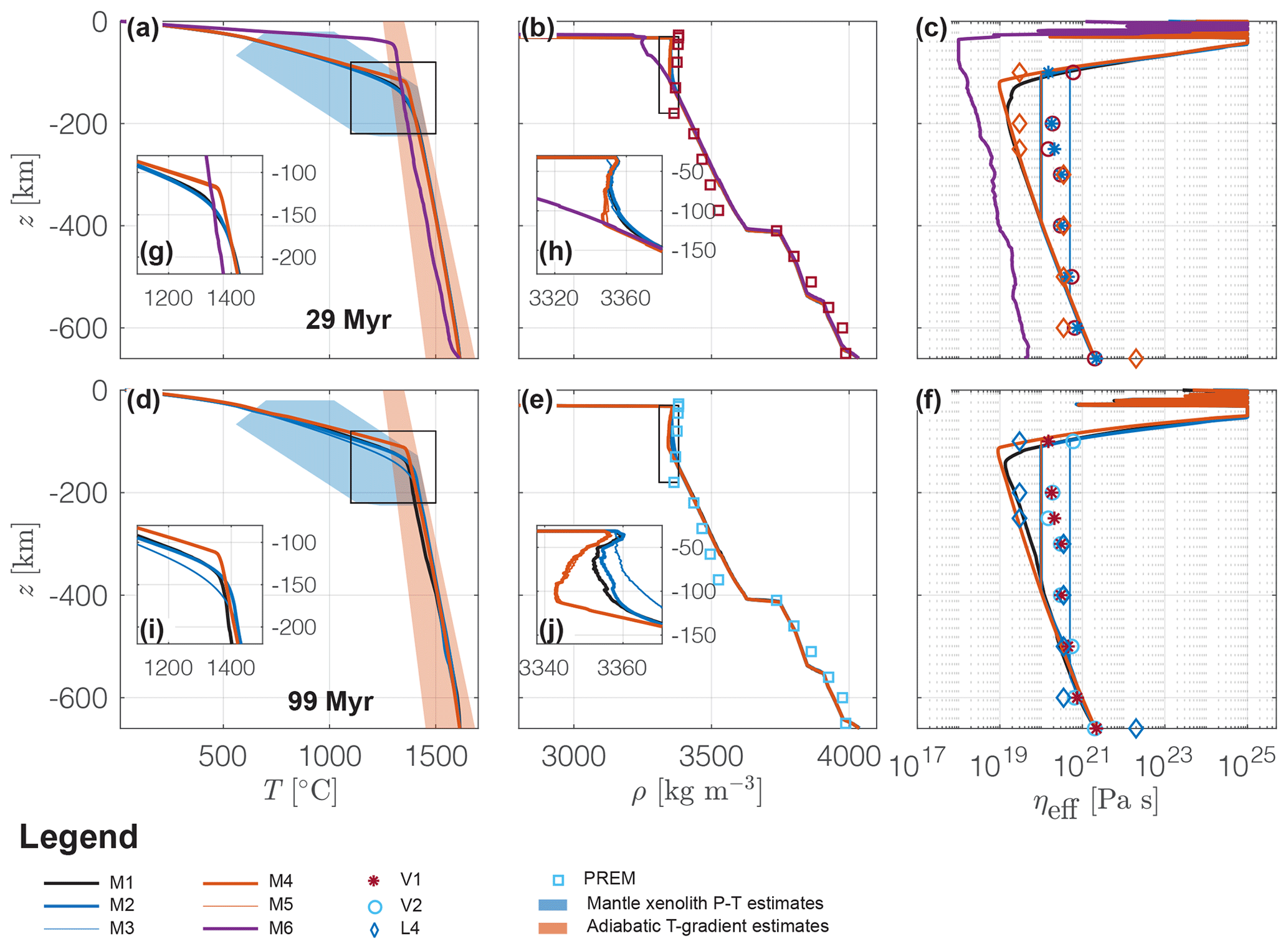
Figure 2 Horizontally averaged vertical profiles of temperature, T, density, ρ, and effective viscosity, η_eff. (a–c) After 29 Myr and (d–f) after 99 Myr in model history. (a, d) Horizontally averaged temperature, (b, e) horizontally averaged density and (c, f) horizontally averaged viscosity. (g–j) An enlargement of the parental subfigure. Coloured lines show the results of models M1–6 as indicated in the legend. In (a, d) the blue area indicates P−T condition estimates from mantle xenolith data, and the orange area indicates estimates for a range of adiabatic gradients, both taken from Hasterok and Chapman (2011) (Fig. 5). Estimates for adiabatic temperature gradients are extrapolated to 660 km of depth. In (b, e) squares indicate density estimates from the preliminary reference Earth model (PREM) (Dziewonski and Anderson, 1981). In (c, f) circles and stars indicate viscosity profiles inferred from Occam-style inversion of glacial isostatic adjustment and convection-related data originally by Mitrovica and Forte (2004); diamonds show a four-layer model fit of mantle flow to seismic anisotropy originally by Behn et al. (2004). All profiles are taken from Forte et al. (2010) (Fig. 2). The median is used as a statistical quantity for averaging because it is less sensitive to extreme values compared to the arithmetic mean.

Figure 3 Model evolution of M1 (reference run). (a, b, c, d) Entire domain. (e, f, g, h) Enlargement. Dark and light blue colours indicate the material phase of weak and strong layers of mica (salmon) and calcite (green) sediments, respectively. White to red colours indicate the effective viscosity field calculated by the algorithm. Arrows represent velocity vectors, and the length of the arrows is not to scale. Scientific colour maps used in all figures are provided by Crameri (2018).

3.2 Wet olivine rheology: model M6

Crustal necking in M6 starts at ca. 2 Myr in model history (Fig. 4a and e). Two convecting cells develop in the horizontal centre of the domain transporting material from z≈-200 km to $z\approx -\mathrm{100}$ km (Fig. 4b and f). At ca. 13 Myr convection cells are active in the upper 500 km of the domain (Fig. 4c). Crustal thickness varies laterally between ca. 20 and <5 km (Fig. 4g). The mantle lithosphere is thermally eroded, indicated by a rising level of the 10²¹ Pa s contour in Fig. 4f–h after 26 Myr in model history. In contrast to M1, M6 does not reach the stage of crustal break-up (Fig. 4d and h) within 30 Myr. Two large convection cells are active: in the left half of the domain convection occurs at relatively enhanced flow speeds, whereas in the right half of the domain flow speeds are relatively lower (compare the relative length of the velocity arrows in Fig. 4d). The average Rayleigh number of the system at this stage is 9.26×10⁷. Values for temperature at the Moho reach ca. 1000 ^∘C locally (Figs. 4h and 2a). The horizontally averaged density profile (Fig. 2b) shows that values for density in the lithosphere are on average 100 kg m⁻³ lower in M6 compared to M1. Values for effective viscosity in the asthenosphere decrease to minimal values of the order of 10¹⁸ Pa s and increase up to values of 10¹⁹ Pa s at a depth of 660 km at the end of the extension period (Fig. 2c).

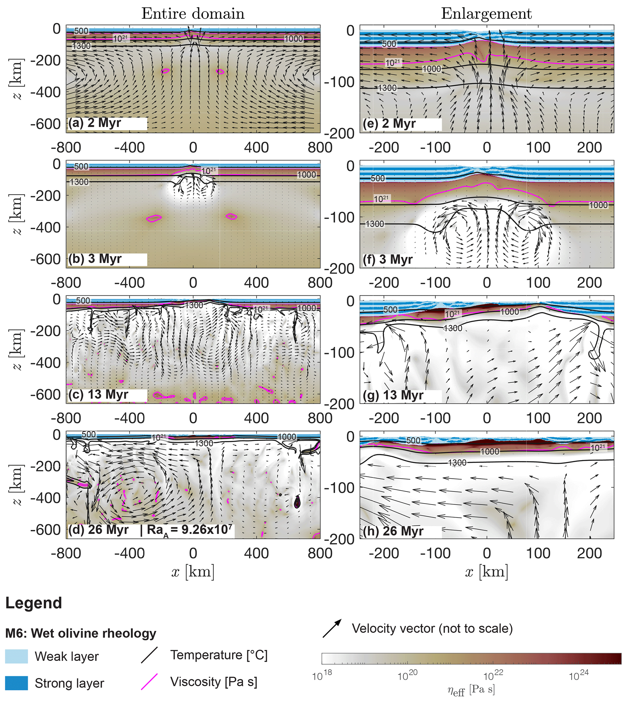
Figure 4 Evolution of model M6 at (a, e) 2 Myr, (b, f) 3 Myr, (c, g) 13 Myr and (d, h) 26 Myr. Blue indicates mechanically weak (light) and strong (dark) crustal units. White to red colours show the effective viscosity field calculated by the numerical algorithm. Black lines show the level of the 500, 1000 and 1300 ^∘C isotherm, and the magenta line shows the level of the 10²¹ Pa s viscosity isopleth. This contour line represents the mechanical boundary between the mantle lithosphere and the convecting upper mantle. Arrows represent velocity vectors, and the length of the arrows is not to scale.

3.3 Comparison of reference run with models M2–5: extension phase

In contrast to M1, M2 produces two conjugate passive margins that are both approximately 150 km long (Fig. 5b) after 13 Myr. Crustal separation has not occurred up to this stage in M3: the two passive margins are still connected by a crustal bridge of ca. 10 km thickness. Mantle material rises below the centre of the domain and then diverges below the plates in M2 and M3, but no convection cells have formed yet (Fig. 5b and c), which is different compared to M1. The minimal value for effective viscosity in the upper mantle is at the applied cut-off value of 1×10²⁰ Pa s in M2 and 5×10²⁰ Pa s in M3 and increases up to ca. 1×10²¹ Pa s at a depth of 660 km (Fig. 2c) in both models. Similar to the reference model (M1), in M4, the left continental margin has a length of ca. 200 km and the right margin has a length of ca. 150 km (Fig. 5d). Like in M1, two convection cells have formed below the two passive margins in this model (see arrows in Fig. 5d); the minimal value for effective viscosity below the lithosphere is of the order of 1×10¹⁹ Pa s and increases to approximately 1×10²¹ Pa s at a depth of 660 km (Fig. 2c). Both margins in M5 are approximately equally long (ca. 150 km, Fig. 5e); values for viscosity are at the lower cut-off value of 1×10²⁰ Pa s in the upper mantle and increase up to ca. 1×10²¹ Pa s at a depth of 660 km (Fig. 2c). The overall evolution of the extension period in M5 is more similar to M2 than to M1. In M1–5, the 1350 ^∘C isotherm does not come closer than ca. 30 km to the surface. Horizontally averaged vertical temperature profiles are similar in M1–5 (Fig. 2a and g). The level of the 1350 ^∘C isotherm remains at its initial depth in M4 and M5, whereas it subsides by ca. 20 km in M1–3. Horizontally averaged density profiles (Fig. 2b) show density differences of <10 kg m⁻³ between ca. 35 and ca. 120 km of depth.

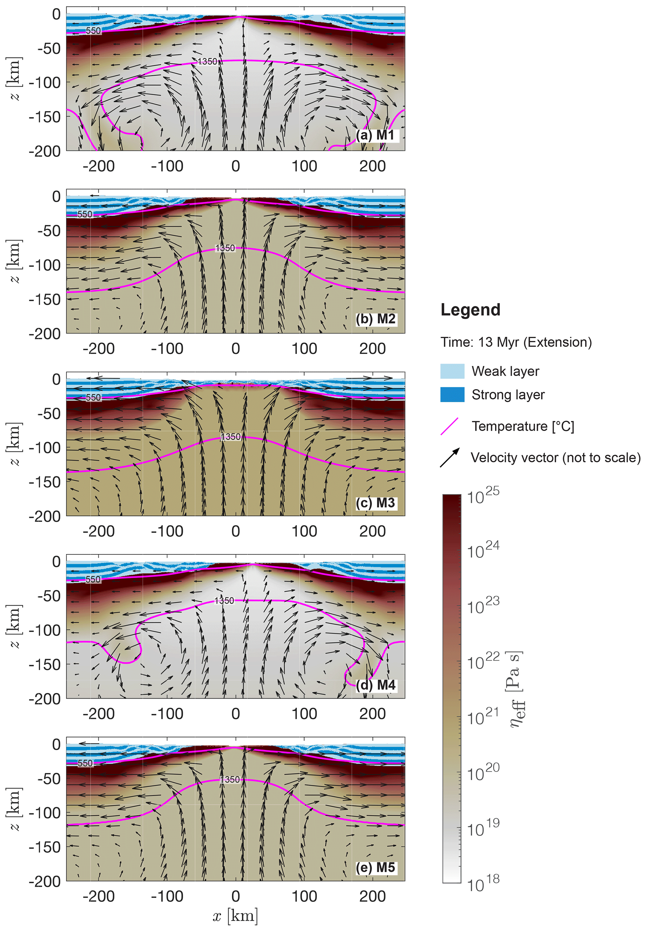
Figure 5 Comparison of M1–5 during the extension stage. (a–e) Enlargements of results of models M1–5 at 13 Myr of modelled time. Blue indicates mechanically weak (light) and strong (dark) crustal units. White to red colours show the effective viscosity field calculated by the numerical algorithm. The magenta lines show the level of the550 and 1350 ^∘C isotherm. Arrows represent velocity vectors, and the length of the arrows is not to scale.

3.4 Comparison of reference run with models M2–5: cooling phase without plate deformation

Models M1–5 maintain a stable lithospheric thickness of ca. 90–100 km over 100 Myr (top magenta viscosity contour in Fig. 6) and no thermal erosion of the lithosphere occurs. Below, the upper mantle is convecting at decreasing Rayleigh numbers from M1 to M5. In M1, the vertical mantle flow speed within the convecting cell at $x\approx +\mathrm{350}$ km is elevated (indicated by the darker blue region in Fig. 6a) compared to the average flow speed of ≈1–2 cm yr⁻¹ in neighbouring cells. The size of the convection cells in M2 is larger compared to M1 and of the order of ca. 100–300 km in diameter. The more elliptical shape of the cells compared to the circular cells in M1 is characteristic. The magnitude of material flow velocity is similar but horizontally distributed more symmetrically below both margins compared to M1 (compare the arrows and colour field in Fig. 6a and b). A zone of strong downward-directed movement develops below both margins (dark blue cells at $x\approx -\mathrm{300}$ km and $x\approx +\mathrm{300}$ km in Fig. 6b). The magnitude of material flow speed is of the order of 1.5 cm yr⁻¹. The average Rayleigh number of the convecting system in M2 is approximately 3.92×10⁶ and is about a factor 2.5 lower compared to M1. M3 develops four large convection cells, two below each margin, that are active up to depths of approximately 600 km (see arrows Fig. 6c). Downward-directed movement of material occurs at ca. 2 cm yr⁻¹ (darker blue regions at $x\approx -\mathrm{500}$ km and x≈500 km in Fig. 6c). The average Rayleigh number of the system is ca. 1.18×10⁶, which is about a factor 8.4 smaller compared to M1. In M4 and M5, material transport occurs at absolute values for vertical velocity <0.5 cm yr⁻¹ (see coloured velocity field in Fig. 6d and e), which is 1 order of magnitude lower compared to M1–3. Two horizontally symmetric convection cells develop in these models that are active between $z\approx -\mathrm{150}$ km and $z\approx -\mathrm{400}$ km (arrows in Fig. 6d and e). The average Rayleigh number is ca. 1.97×10⁶ and 5.48×10⁵ in M4 and M5, respectively. Figure 6f–j show the difference between the entire density field and the horizontally averaged vertical density profile at 99 Myr (see Fig. 2e), and Fig. 7b shows a horizontal profile of this field averaged vertically over $-\mathrm{200}\le z\le -\mathrm{100}$ km. The distribution of density differences becomes more horizontally symmetric with decreasing Rayleigh number (M1–5; see Fig. 7b). In M1, the 2 kg m⁻³ density contour line encloses a high-density anomaly below the right passive margin (see black contour line at x≈300 km, $z\approx -\mathrm{200}$ km in Fig. 6f). Calculating the suction, or buoyancy, force for this body according to Eq. (D4) yields a value of 0.25 TN m⁻¹. Since the distribution of density differences is laterally symmetric in M2–5 (Fig. 7b) and defining an integration area is not trivial, a calculation of suction forces is not attempted for M2–5. Figure 7a shows the topography at ca. 99 Myr in model history, which is 1 Myr before the start of convergence. Topography does not exceed 1.5 km and the average depth of the basin is ca. 3.75 km.

Figure 6 Results of models M1–5 at 99 Myr (end of cooling period). (a–e) Blue to red colours indicate the vertical velocity magnitude calculated by the numerical algorithm. Black arrows velocity vectors show (not to scale) to visualize the material flow field. (f–j) Blue to red colours indicate the difference between the entire density field and the horizontal average density profile as shown in Fig. 2e. Black lines are the 2 kg m⁻³ density contour. The magenta line shows the level of the 10²¹ Pa s viscosity isopleth in all subfigures. This contour line represents the mechanical boundary between the rigid mantle lithosphere (no velocity glyphs) and the convecting upper mantle.

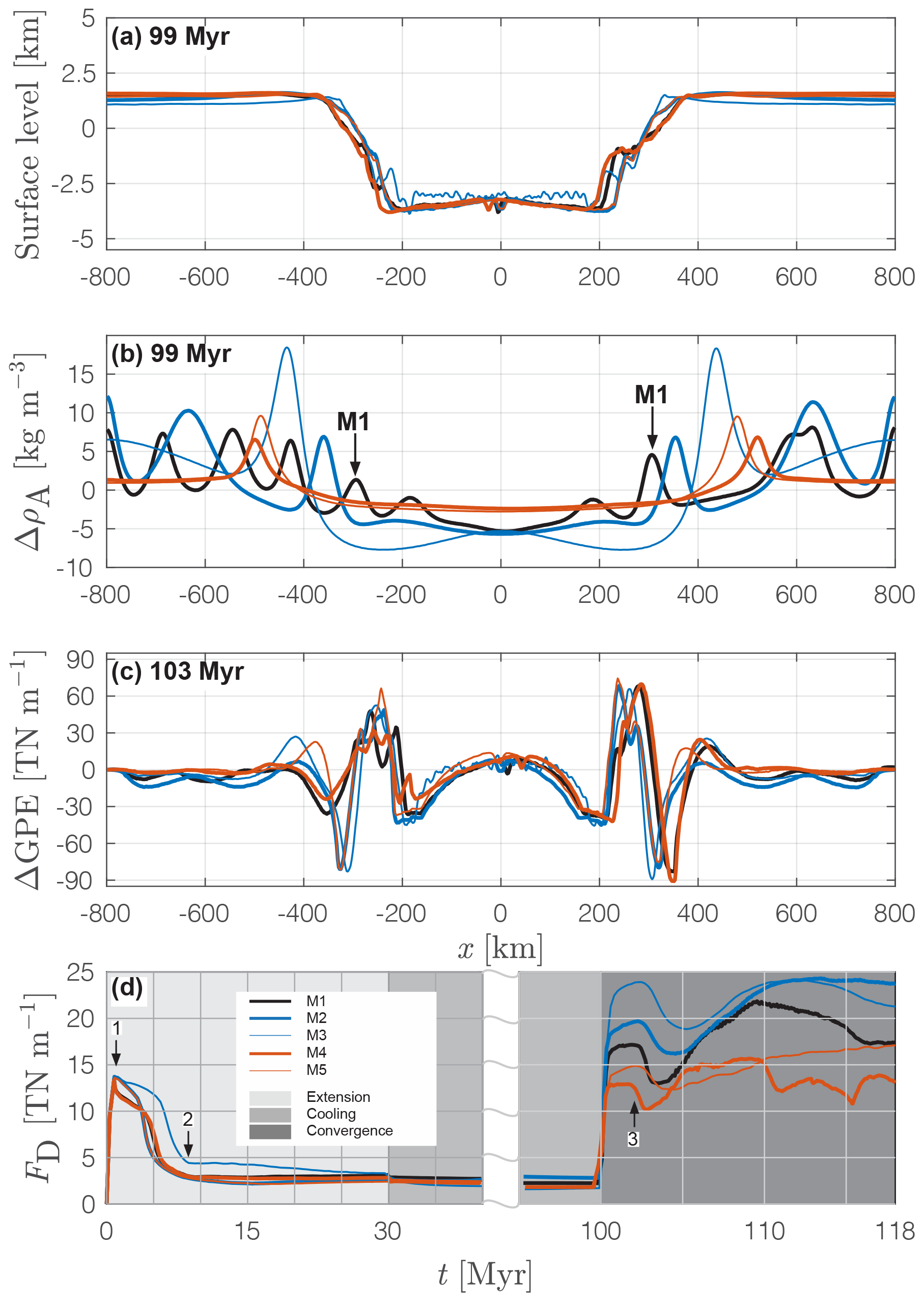
Figure 7 (a) Model topography at the end of the cooling period. (b) Vertically averaged ($-\mathrm{200}\mathrm{km}\le z\le -\mathrm{100}\mathrm{km}$) difference between the entire density field and horizontal average density (see also Fig. 6(f–j). (c) Difference in GPE of models M1–5 after 103 Myr. (d) Estimated plate driving forces (F_D, see Appendix D) through the entire model time. Grey regions indicate the stages of extension (light grey), cooling without plate deformation (grey) and convergence (dark grey). The cooling period is not entirely displayed because values for F_D remain constant when no deformation is applied to the system. Numbers indicate important events in the evolution of the models: 1: initiation of crustal necking, 2: crustal break-up, opening of the marine basin in which the mantle is exhumed to the sea floor, 3: subduction initiation via thermal softening. The legend shown in (d) is valid for all panels above as well.

Figure 8a–e show the conductive heat flow of the entire domain in absolute values. Models M1–5 reproduce a heat flux of 20–30 mW m⁻² through the base of the lithosphere (indicated by the 10²¹ Pa s isopleth at a depth between 100 and 110 km). The conductive heat flow below the lithosphere is close to 0 mW m⁻² in M1–3. In M4 and M5, values for conductive heat flow remain at ca. 20 mW m⁻² through the entire upper mantle. Density differences in the upper part of the mantle lithosphere reach ca. 20 kg m⁻³ between ca. 35 and 120 km in depth (Fig. 2e and j). Values for effective viscosity are of the order of 10¹⁹ Pa s for M1 and M5 and of the order 10²⁰ Pa s in M2–4 directly below the lithosphere and 10²¹ Pa s at the bottom of the upper mantle (Fig.  2f).

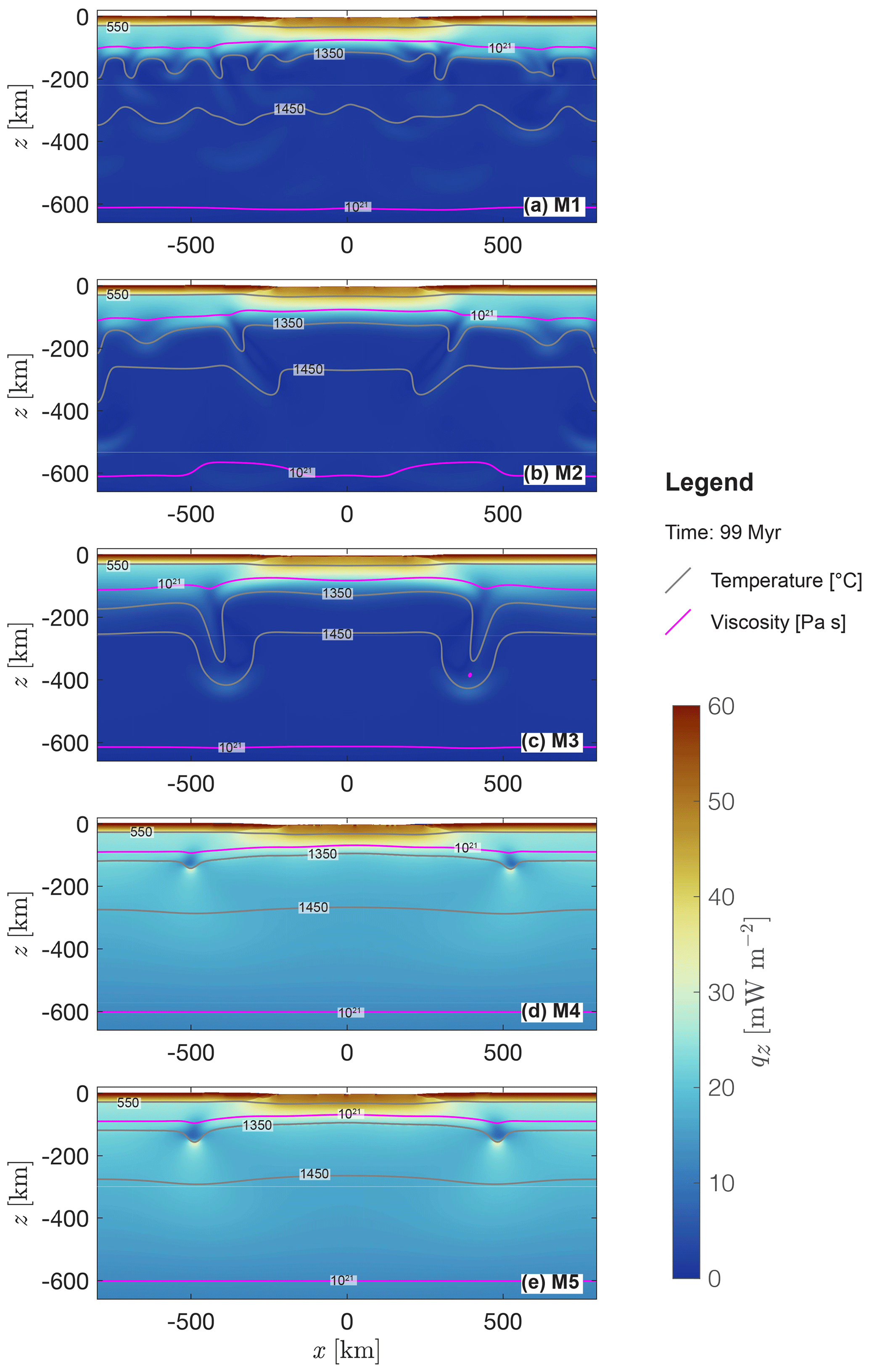
Figure 8 Vertical conductive heat flow represented by blue to red colours for models M1–5 (a–e) after 99 Myr. The grey lines indicate the depth of the 550, 1350 and 1450 ^∘C isotherm. The magenta line indicates the depth of the 10²¹ Pa s isopleth, which approximately represents the mechanical transition between the mantle lithosphere and the convecting upper mantle.

3.5 Comparison of reference run with models M2–5: convergence and subduction phase

In contrast to M1, two major symmetric shear zones develop in the lithosphere in M2, M3 and M5, one shear zone at each of the continental margins (Fig. 9b, c and e). Like in M1, one shear zone forms below the right margin in M4 (Fig. 9d). At this early stage of subduction initiation, the strain rate in the shear zone is of the order 10⁻¹⁴–10⁻¹³ s⁻¹. In the region of the shear zones, the temperature is increased, which is indicated by the deflection of the isotherms (red contour lines in Fig. 9a–e). Horizontal profiles of gravitational potential energy (GPE; see Appendix D) are in general similar (Fig. 7c) for M1–5.

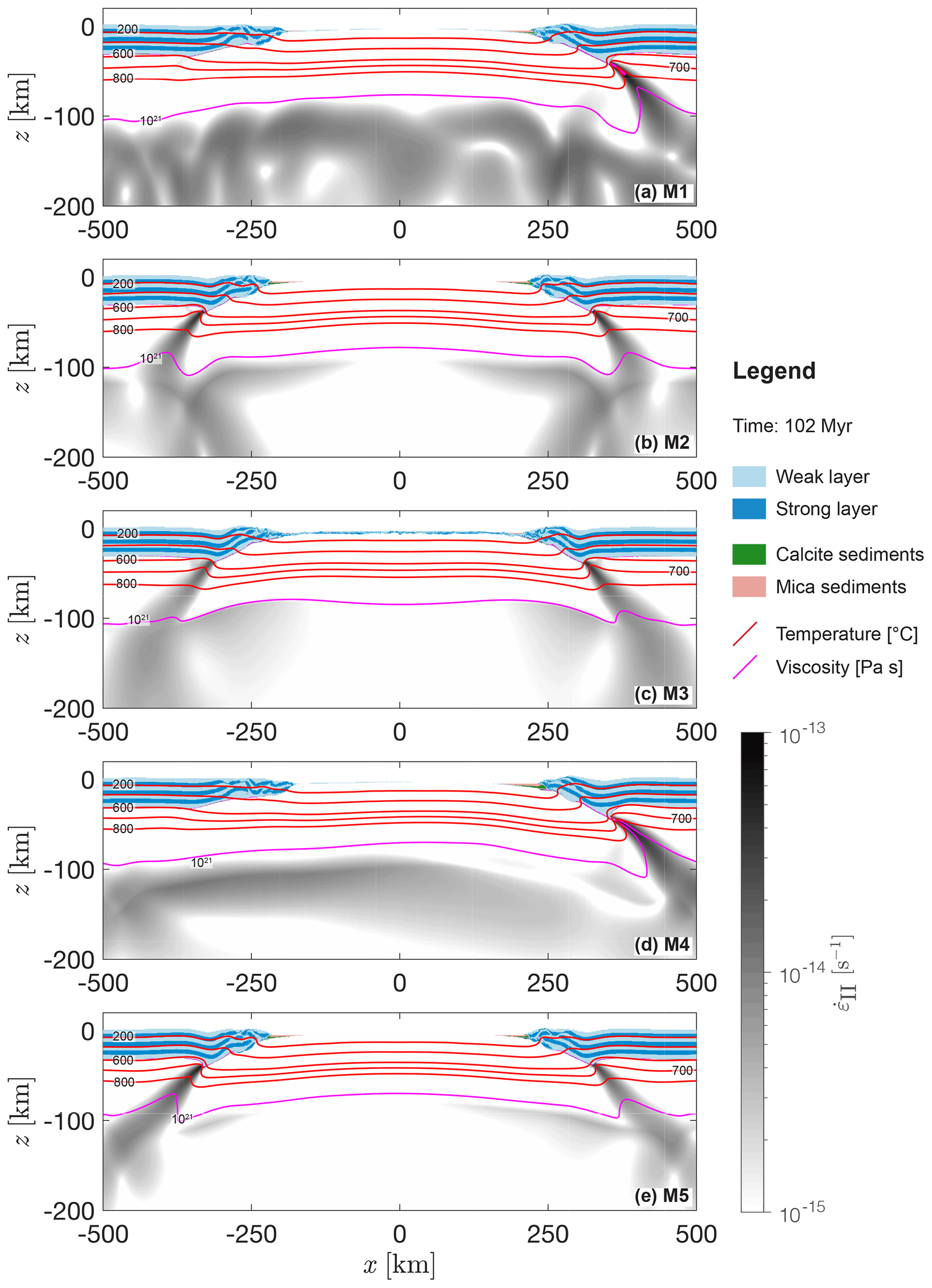
Figure 9 Stage of subduction initiation. (a–e) Results of models M1–5 after 102 Myr of simulated deformation. Blue indicates mechanically weak (light) and strong (dark) crustal units, and green and salmon indicate the sedimentary units (only minor volumes in trench regions). White to black colours indicate the second invariant of the strain rate tensor field calculated by the numerical algorithm. Red lines show levels of several isotherms, and the magenta line shows the level of the 10²¹ Pa s viscosity isopleth. This contour line approximately represents the mechanical transition between the mantle lithosphere and the convecting upper mantle.

In contrast to the single-slab subduction evolving in M1, double-slab subduction is observed below both margins in M2–5 and sediments are deposited in two trenches as the subduction evolves (Fig. 10b–e). Folding of the crustal layers indicates deformation in both margins of M2–5. Values for viscosity in the upper mantle remain stable at values of 10¹⁹ Pa s in M4, whereas the viscosity values are at the applied lower cut-off value in M2, M3 and M5 throughout the entire simulation history. Convection cells remain active during subduction. Similar to M1, a stable convection cell is active below one subducting slab in M4. The distribution of convection cells is more symmetric in front of the slabs in M2, M3 and M5 compared to M1. Defined by the applied boundary condition, material flows into the model domain up to $z=-\mathrm{330}$ km at the lateral boundaries in all models (see Sect. 2.2). However, far away from the boundary in the centre of the domain in M1 and M2 the horizontal material inflow from the lateral boundaries is limited up to a depth of ca. 100–150 km (see horizontally directed arrows in Fig. 10a and b). In M3–5 the lateral inflow of material reaches a depth of about 200 km in the centre of the domain (Fig. 10c–e).

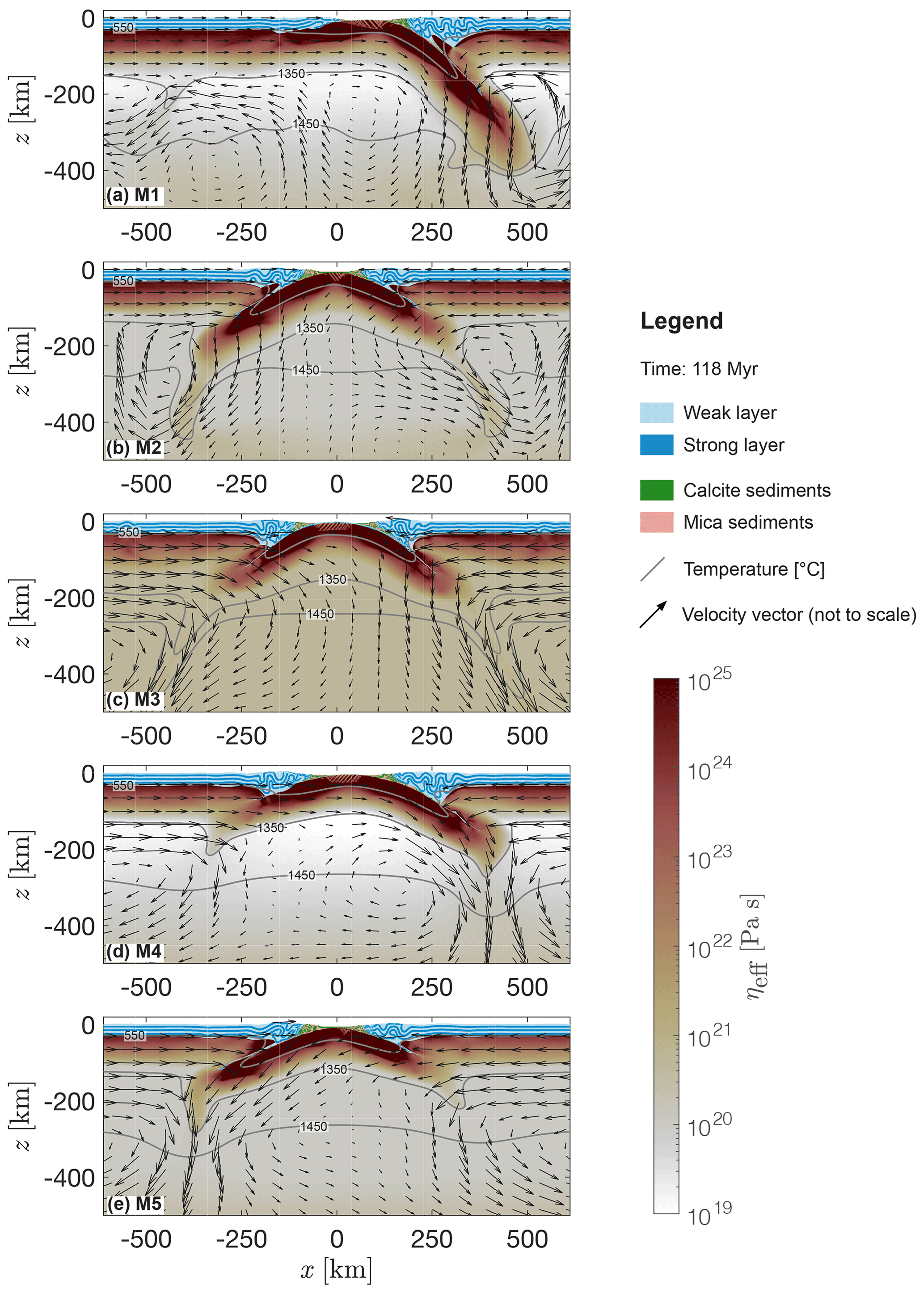
Figure 10 Evolution of subduction zones. (a–e) Results of models M1–5 after 118 Myr of simulated deformation. Blue indicates mechanically weak (light) and strong (dark) crustal units, and green and salmon indicate the sedimentary units. White to red colours show the effective viscosity field calculated by the numerical algorithm for the mantle lithosphere and the upper mantle. Arrows represent velocity vectors, and the length of the arrows is not to scale. Grey lines indicate the 550, 1350 and 1450 ^∘C isotherm.

3.6 Estimates for plate driving forces

The vertically integrated second invariant of the deviatoric stress tensor, ${\stackrel{\mathrm{‾}}{\mathit{\tau }}}_{\mathrm{II}}$, is a measure for the strength of the lithosphere, and twice its value is representative for the horizontal driving force (per unit length, F_D hereafter) during lithosphere extension and compression (Appendix D). Figure 7d shows the evolution of F_D during the entire cycle. During the pure shear thinning phase in the first ca. 2 Myr of extension, values for F_D reach 14 TN m⁻¹. At ca. 2–3 Myr (1 in Fig. 7d), this value drops below ca. 5 TN m⁻¹ at ca. 8 Myr. At the end of the extension period F_D is stabilized at values between ca. 2 and 3 TN m⁻¹ for all models (2 in Fig. 7d). This value remains relatively constant for all models during the entire cooling period. The maximum value for F_D necessary to initiate subduction in all models is observed in M3 and is ca. 23 TN m⁻¹ (thin blue curve in Fig. 7d). The minimum value necessary for subduction initiation of ca. 13 TN m⁻¹ is observed in M4. The reference run M1 initiates subduction with a value of F_D≈17 TN m⁻¹. Strain localization at ca. 102 Myr is associated with a rapid decrease in F_D by ca. 2–5 TN m⁻¹ in all models (3 in Fig. 7d). At ca. 105 Myr, values for F_D increase again until the end of the simulation.

4 Discussion

4.1 Impact of mantle viscosity structure and effective conductivity on passive margin formation

Higher values for the lower viscosity cut-off (M2 and M3 compared to M1) not only change the viscosity structure of the mantle, but also increase the strength of the weak layers. In consequence, the multilayered crust effectively necks as a single layer. The resulting passive margins are slightly shorter and more symmetric (Duretz et al., 2016b, see also M3). The highest cut-off value of 5×10²⁰ Pa s (M3) leads to a two-stage necking as investigated by Huismans and Beaumont (2011). First, the lithosphere necks while the crust deforms by more or less homogeneous thinning, leading to the development of a large continuous zone of hyperextended crust, below which the mantle lithosphere has been removed. Second, the hyperextended crust breaks up later than the continental mantle lithosphere. During the rifting stage, the thermal field in all simulations is very similar (see Fig. 2a), presumably because effects of heat loss due to diffusion are not significant over the relatively short timescale.

4.2 Onset of upper mantle convection and thermo-mechanical evolution of the lithospheric plates

Rifting in M1–5 causes upwelling of hot asthenospheric material in the horizontal centre of the domain. The resulting lateral thermal gradients are high enough to induce small-scale convection (Buck, 1986). Huang et al. (2003) derived scaling laws to predict the onset time for small-scale convection in 2D and 3D numerical simulations. They investigated the impact of plate motion, layered viscosity, temperature perturbations and surface fracture zones on the onset time. The observed onset time in layered viscosity systems becomes larger when the thickness of the weak asthenosphere decreases. Also, plate motion can delay the onset of small-scale convection. In contrast, fracture zones at the surface may lead to earlier onset of convection depending on the thermal structure of the fracture zones. Using their scaling law and the parameters used in our reference model M1, the onset time of convection is predicted for ca. 43 Myr. However, the onset of convection in M1 is observed as early as ca. 8 Myr (see Fig. 3), which is consistent with onset times observed in numerical simulations conducted by Van Wijk et al. (2008). There may be several reasons for the discrepancy between the prediction and observation. First, the models presented here are likely a combination of the configurations tested by Huang et al. (2003). Second, the choice of boundary conditions and initial configuration is different, which is probably important when testing the impact of plate motion on the onset time. They located the rift centre at the left lateral boundary, whereas the rift centre in our models is located far away from the lateral boundaries in the horizontal centre of the domain. This likely impacts the flow direction of hot material ascending beneath the rift centre and consequently alters lateral thermal gradients, which are important for the onset of convection. The onset time for convection is delayed and occurs at ca. 20 Myr in M2 and at ca. 30 Myr in M3. This delay is likely due to the increased viscosity in the asthenosphere in M2 and M3 compared to M1, which decreases the Rayleigh number of the system. This observation is in agreement with the general inverse proportionality of the onset time of convection to the Rayleigh number as predicted by Huang et al. (2003).

Once convection has started, it stabilizes the temperature field (Richter, 1973; Parsons and McKenzie, 1978) over large timescales and controls the thickness of the lithosphere. Although we allow for material inflow up to $z=-\mathrm{330}$ km, the arrows in Fig. 10a and b indicate that lateral inflow of material far away from the boundary is limited up to $z>\approx -\mathrm{150}$ km. Below this coordinate, the convection cells even transport material towards the lateral boundary in the opposite direction of material inflow. This observation suggests that the thermal thickness of the lithosphere adjusts self-consistently and far away from the boundary during the geodynamic cycle. The thermal thickness of the lithosphere seems to vary with decreasing Rayleigh number: in M5 the value for the thermal thickness of the lithosphere is ≈200 km (see arrows in Fig. 10e). This observation suggests that the thermal thickness of the moving lithosphere is presumably regulated by the vigour of convection.

For realistic values for thermal conductivity in the upper mantle (M1–3), heat flow through the base of the mechanical lithosphere is between 20 and 30 mW m⁻² (Fig. 8a–c). These values are in the range of heat flow estimates for heating at the base of the lithosphere confirmed by other numerical studies (Petersen et al., 2010; Turcotte and Schubert, 2014). Below the lithosphere, the conductive heat flux is essentially zero because heat transport is mainly due to advection of material in the convecting cells. The effective conductivity approach maintains a reasonable heat flux directly at the base of the lithosphere (Fig. 8d and e) and convection cells develop. However, all processes in the upper mantle are conduction-dominated (see elevated values for q_z in Fig. 8d and e). This implies that the characteristic physics of mantle convection are not captured correctly in these models. This becomes evident when comparing Fig. 6a to Fig. 6d: although the physical parameters – except the thermal conductivity in the upper mantle – are the same in both simulations and temperature profiles are similar (see Fig. 2d and i), the Rayleigh numbers of the systems differ by 1 order of magnitude (see Table 1) and the convective patterns are entirely different.

4.3 Mantle convection, thermal erosion and tectonics in the Archean

Model M6 underlines the importance of better constraining the rheology of the mantle. Due to significantly reduced viscosities (see Fig. 2c), convection in the upper mantle occurs at an average Rayleigh number of ca. 9×10⁷ in M6. Compared to estimates for present-day Earth's upper mantle convection (Torrance and Turcotte, 1971; Schubert et al., 2001) this Rayleigh number is an order of magnitude higher. The lithosphere is recycled rapidly and the resulting values for density directly below the lithosphere are ca. 100 kg m⁻³ lower in M6 compared to M1–5. The resulting density structure in the upper region of the mantle deviates significantly from the PREM (Dziewonski and Anderson, 1981, see Fig. 2b). Convection at such high Rayleigh numbers leads to an enhanced temperature field. Resulting values for temperature at the Moho locally reach ca. 1000 ^∘C. Our models suggest that such weak mantle rheology is actually not feasible for present-day plate tectonics, but this non-feasibility can only be observed when performing coupled mantle–lithosphere models as we have presented. In lithosphere-only models, a weak mantle would not generate the thermal erosion of the lithosphere bottom as observed in model M6 because the lithosphere bottom would be “stabilized” by the bottom boundary condition. In the Archean eon, the mantle potential temperature was probably 200–300 ^∘C higher (Herzberg et al., 2010) and therefore convection was more vigorous (Schubert et al., 2001). Agrusta et al. (2018) have investigated the impact of variations in mantle potential temperature compared to present-day values for slab dynamics. Assuming a 200 ^∘C higher value for the mantle potential temperature compared to present-day estimates leads to viscosity structures similar to the average viscosity structure we report for M6 (compare Fig. 6c in Agrusta et al., 2018, to Fig. 2c in this study). Hence, we argue that such vigorously convecting systems as presented in M6 may be applicable to the mantle earlier in Earth's history.

4.4 Spontaneous vs. induced subduction initiation and estimates for plate driving forces

Currently, the processes and tectonic settings leading to subduction initiation remain unclear (Stern, 2004; Stern and Gerya, 2018; Crameri et al., 2019). Stern (2004) proposed two fundamental mechanisms for subduction initiation.

• 1.

  The first is that spontaneous (or vertically forced; Crameri et al., 2020) subduction initiation occurs, for example, due to densification of the oceanic lithosphere during secular cooling. Cloos (1993) proposed that the density increase of a cooling, 80 Myr old oceanic lithosphere compared to the underlying asthenosphere is of the order of 40 kg m⁻³. According to Cloos (1993), this difference is sufficient to spontaneously initiate subduction through negative buoyancy of the oceanic lithosphere (see Stern, 2004, Stern and Gerya, 2018, and references therein for detailed explanation). However, McKenzie (1977) and Mueller and Phillips (1991) showed that the forces acting on the lithosphere due to buoyancy contrasts are not high enough to overcome the strength of the cold oceanic lithosphere. Observations of old plate ages (>100 Myr) around passive margins in the South Atlantic (Müller et al., 2008) indicate their long-term stability.

  In the models presented here, the applied thermodynamic density of the Hawaiian pyrolite leads to density differences between the exhumed mantle in the basin and the underlying asthenosphere of ca. 10–20 kg m⁻³ after 99 Myr in model history. These buoyancy contrasts are ca. 2 times smaller than the contrast proposed by Cloos (1993). Boonma et al. (2019) calculated a density difference (ρ_ast−ρ_lit) of +19 kg m⁻³ for an 80 km thick continental lithosphere and −17 kg m⁻³ for an oceanic lithosphere 120 Myr old. These values are in agreement with the values we report in our study. In the 2D models presented here, these buoyancy contrasts are insufficient to overcome the internal strength of the cooled exhumed mantle and spontaneously initiate subduction at the passive margin.

  However, modelling spontaneous subduction initiation for an ad hoc constructed passive margin geometry is possible if the employed mechanical resistance is small, the density difference between lithospheric and oceanic mantle is large, and/or if an additional weak zone is imposed. Such passive margin configurations are indeed unstable and lead to spontaneous subduction initiation within a few million years (Stern and Gerya, 2018, and references therein). However, the passive margins we consider in our study have been stable for at least 60 Myr before subduction initiation. Therefore, spontaneous subduction initiation for unstable passive margins is in contrast with the observation of long-term stability of the ancient Alpine Tethys margins (McCarthy et al., 2018) and the recent passive margins in the South Atlantic (Müller et al., 2008). Our results are hence in agreement with the stability of these passive margins. Modelling long-term geodynamic cycles, applicable to the evolution of the Alpine Tethys and the South Atlantic, requires appropriate density and rheological models which generate passive margins that are stable for more than 60 Myr (Alpine Tethys) or more than 180 Myr (South Atlantic). To evaluate whether models of spontaneous SI at passive margins are feasible, these models need to explain why the passive margins have been stable for more than 60 Myr and only afterwards spontaneously “collapsed”, although they are cooled and mechanically strong.

• 2.

  The second is that induced (or horizontally forced; Crameri et al., 2020) subduction initiation occurs, for example, due to far-field plate motion. In fact, many numerical studies that investigate subduction processes do not model the process of subduction initiation. In these studies, a major weak zone across the lithosphere is usually prescribed ad hoc in the initial model configuration to enable subduction (Ruh et al., 2015; Zhou et al., 2020). Another possibility to model subduction is to include a prescribed slab in the initial configuration. This means that subduction has already initiated at the onset of the simulation (Kaus et al., 2009; Garel et al., 2014; Holt et al., 2017; Dal Zilio et al., 2018). In our models, subduction is initiated self-consistently, which means that (i) we do not prescribe any major weak zone or an already existing slab, and (ii) the model geometry and temperature field at the onset of convergence (100 Myr) were simulated during a previous extension and cooling phase with the same numerical model and parameters. Subduction is initiated during the initial stages of convergence and subduction initiation is hence induced by horizontal shortening. Notably, Crameri et al. (2020) analysed more than a dozen documented subduction zone initiation events from the last hundred million years and found that horizontally forced subduction zone initiation is dominant over the last 100 Myr. During convergence in our models, shear heating together with the temperature- and strain-rate-dependent viscosity formulation (dislocation creep flow law, Eq. A7) cause the spontaneous generation of a lithosphere-scale shear zone that evolves into a subduction zone (Thielmann and Kaus, 2012; Kiss et al., 2020). However, shear heating is a transient process, which means the increase in temperature is immediately counterbalanced by thermal diffusion. Efficiency of shear heating is restricted to the first ca. 2–3 Myr after shear zone formation in the presented models. After this time span, heat generated by mechanical work is diffused away. Therefore, thermal softening is unlikely the mechanism responsible for stabilization of long-term subduction zones, but it is likely important for initiating and triggering subduction zones.

  The value of F_D (see Appendix D) represents the plate driving force. In M1, the maximal value of F_D just before stress drop caused by subduction initiation at ≈103 Myr is ≈17 TN m⁻¹ (Fig. 7d). However, F_D≈2 TN m⁻¹ at the end of the cooling stage, resulting from stresses due to mantle convection and lateral variation of GPE between the continent and basin. Therefore, this value can be subtracted from the ≈17 TN m⁻¹. The required plate tectonic driving force for convergence-induced subduction initiation is then ≈15 TN m⁻¹ for M1. Kiss et al. (2020) modelled thermal-softening-induced subduction initiation during convergence of a passive margin, whose geometry and thermal structure were generated ad hoc as an initial model configuration. Their initial passive margin structure was significantly less heterogeneous than ours. To initiate subduction, they needed a driving force of ≈37 TN m⁻¹, which is significantly larger than the ≈15 TN m⁻¹ required in our model M1. Obviously, the ≈15 TN m⁻¹ cannot be exceeded by the mantle convection (≈2 TN m⁻¹) modelled here. Even assuming an additional ridge push force of 3.9 TN m⁻¹ (Turcotte and Schubert, 2014) would not be sufficient to spontaneously initiate subduction in the models presented here. The boundary convergence providing the remaining ca. 9 TN m⁻¹ to initiate subduction in our models is assumed to be caused by far-field plate driving forces. These are generated by global processes that are not modelled inside our domain, such as slab pull, whole-mantle convection and ridge push. For example, the closure of the Piemonte–Liguria basin is assumed to be caused by the much larger-scale convergence of the African and European plates (McCarthy et al., 2018).

  We suggest that mechanical and geometrical heterogeneity inherited by previous deformation periods and thermal heterogeneity due to mantle convection reduces the required driving force necessary for subduction initiation by thermal softening. Additionally, we suppose that the plate driving force necessary for horizontally forced subduction initiation in our models could be further reduced by considering more heterogeneities or a smaller yield stress in the mantle lithosphere. However, the minimum value for F_D, which can still generate horizontally forced subduction initiation via thermal softening, has to be quantified in future studies. This is relevant because the main argument against thermal softening as an important localization mechanism during lithosphere strain localization and subduction initiation is commonly that the required stresses, and hence driving forces, are too high. In nature, more softening mechanisms act in concert with thermal softening, such as grain damage (e.g. Bercovici and Ricard, 2012; Thielmann and Schmalholz, 2020), fabric and anisotropy evolution (e.g. Montési, 2013), and reaction-induced softening (e.g. White and Knipe, 1978), likely further reducing forces required for subduction initiation. Furthermore, Mallard et al. (2016) showed with 3D spherical full-mantle convection models that a constant yield stress between 150 and 200 MPa in their outer boundary layer, representing the lithosphere, provides the most realistic distribution of plate sizes in their models. The yield stress in their models corresponds to a deviatoric von Mises stress, which is comparable to the value of τ_II calculated for our models. If we assume a 100 km thick lithosphere, then F_D=15 TN m⁻¹ yields a vertically averaged deviatoric stress, τ_II, of 75 MPa for our model lithosphere. Therefore, vertically averaged deviatoric stresses for our model lithosphere are even smaller than deviatoric, or shear, stresses employed in global mantle convection models. Based on the above-mentioned arguments, we propose that ≈15 TN m⁻¹ is a feasible value for the horizontal driving force per unit length.

4.5 Mantle convection stabilizing single-slab subduction

Figure 7c shows the difference in GPE at 103 Myr. The horizontal profiles do not reveal significant differences between the models. The GPE is sensitive to topography and density distribution throughout the model domain. Values for density differences are ca. 10–20 kg m⁻³ across the mantle lithosphere. When integrated over the entire depth, such variations do not significantly impact the GPE profiles. Instead, the signal reflects the topography, which is similar in all the models due to the similar margin geometry (see Figs. 7a and 5a–e). In consequence, stress concentrations lead to localized deformation and shear zone formation at both margins in all models during the onset of convergence. Therefore, the evolution and stabilization of a single-sided subduction requires an additional asymmetry of the system.

The average Rayleigh number (see Appendix Eq. B1) in M1 is ca. 9.95×10⁶ (see Table 1), which is close to estimated values for upper mantle convection (Torrance and Turcotte, 1971; Schubert et al., 2001). Potential lateral asymmetry caused by the convecting cells in the upper mantle is inherited from the cooling period. The vertical velocity field at the end of the cooling period of M1 (Fig. 6a) reveals one convection cell at $x\approx +\mathrm{350}$ km with flow speeds of the order of the convergence velocity applied later. This convection cell is induced by a high-density anomaly directly below the passive margin at which subduction will be initiated later in the model (see the black contour line below the right margin in Fig. 6f). This sinking, high-density body probably induces an asymmetry in the form of an additional suction force exerted on the lithospheric plate. Conrad and Lithgow-Bertelloni (2002) quantified the importance of slab pull vs. slab suction force and showed that the slab pull force and the suction force of a detached slab sinking into the mantle induce similar mantle flow fields. They argued that a detached fraction of a slab sinking into the mantle can exert shear traction forces at the base of the plate and drive the plate. Baes et al. (2018) showed with numerical simulations that sinking of a detached slab below a passive margin can significantly contribute to the initiation of subduction. We suggest that the high-density anomaly observed in M1 and the associated mantle flow also generate a force similar to a slab suction force. To quantify the suction force induced by the sinking, high-density body in M1, we calculated the difference of the density in this region with respect to the horizontally averaged density field presented in Fig. 2e and spatially integrated this buoyancy difference over the area enclosed by the 2 kg m⁻³ density contour below the right passive margin (see Fig. 6f). The resulting buoyancy force per unit length is ca. 0.25 TN m⁻¹. This value is relatively low compared to the plate driving forces acting in the model, but it likely induces a sufficiently high asymmetry to stabilize the single-slab subduction in simulation M1.

Values for the Rayleigh number in M2 and M3 are lower (3.92×10⁶ and 1.18×10⁶, respectively) compared to M1 (see Table 1) because of the relatively higher viscosity (see Eq. B1). With decreasing Rayleigh number the asymmetry of convection also decreases (Schubert et al., 2001). In consequence, the size of the convecting cells becomes larger and more elliptic (M2 compared to M1) and the number of active cells decreases (M3 compared to M1). Enhancing the thermal conductivity (included in the denominator in Eq. B1) by ca. 1 order of magnitude in models M4 and M5 also decreases the Rayleigh number by 1 order of magnitude compared to M1 (see Table 1). Decreasing the Rayleigh number (M2–5) leads to more laterally symmetric convective flow patterns and decreases the speed and distribution of material flow (see Fig. 6b–e). In turn, this probably leads to more equally distributed density differences (Fig. 7b) and therefore suction forces exerted on the plates. Hence, we argue that decreasing the Rayleigh number, assuming a relatively strong asthenosphere or applying an enhanced thermal conductivity likely favours the initiation of divergent double-slab subduction. The resulting slab geometries resemble a symmetric push-down (M2–5) rather than a stable asymmetric subduction (M1). This impacts the deformation in the lithosphere, especially in the crust: the crustal layers of both plates are strongly folded (see Fig. 10b–e). In M1, the deformation of the crustal layers only occurs in the overriding plate.

4.6 Comparison with estimates of Earth's mantle viscosity and thermal structure

To apply our models to geodynamic processes on Earth, we compare several model quantities with measurements and indirect estimates of these quantities. Even after 118 Myr of model evolution, the mantle density structure of our model remains in good agreement with the preliminary reference Earth model (PREM; Dziewonski and Anderson, 1981, see Fig. 2b and e). The geotherm of the conduction dominated regime remains well in the range of pressure–temperature (P−T) estimates from mantle xenolith data. Also, the geotherm of the convection-dominated regime remains within the range for adiabatic gradients and potential temperatures applicable to the Earth's mantle (Hasterok and Chapman, 2011; see Fig. 2a and d) during the entire long-term cycle. Viscosity profiles lie within the range of estimates inferred by inversion of observable geophysical data and from experimentally determined flow law parameters of olivine rheology (Mitrovica and Forte, 2004; Behn et al., 2004; Hirth and Kohlstedt, 2003, see Fig. 2c and f). Lithosphere and mantle velocities are in a range of several centimetres per year, which is in agreement with predictions from boundary layer theory of layered mantle convection (Schubert et al., 2001) and plate velocity estimates from GPS measurements (Reilinger et al., 2006).

4.7 Formation and reactivation of magma-poor rifted margins: potential applications

Our model can be applied to some first-order geodynamic processes that were likely important for the orogeny of the Alps. Rifting in the Early to Middle Jurassic (Favre and Stampfli, 1992; Froitzheim and Manatschal, 1996; Handy et al., 2010) led to the formation of the Piemont–Liguria ocean, which was bounded by the hyperextended magma-poor rifted margins of the Adriatic plate and the Briançonnais domain on the side of the European plate. We follow the interpretation that the Piemont–Liguria ocean was an embryonic ocean which formed during ultra-slow spreading and was dominated by exhumed subcontinental mantle (e.g. Picazo et al., 2016; McCarthy et al., 2018; Chenin et al., 2019; McCarthy et al., 2020). If true, there was no stable mid-ocean ridge producing an ocean several hundred kilometres wide with a typically 8 km thick oceanic crust, and our model would be applicable to the formation of an embryonic ocean with an exhumed mantle bounded by magma-poor hyperextended rifted margins. Our models show the formation of a basin with an exhumed mantle bounded by hyperextended margins above a convecting mantle. Hence, our model may describe the first-order thermo-mechanical processes during formation of an embryonic ocean. During closure of the Piemont–Liguria ocean, remnants of those magma-poor ocean–continent transitions escaped subduction and are preserved in the eastern Alps (Manatschal and Müntener, 2009). We follow the interpretation that the initiation and at least the early stages of ocean closure were caused by far-field convergence between the African and European plates (e.g. Handy et al., 2010). We further assume that subduction was induced, or horizontally forced, by this convergence and was not spontaneously initiated due to buoyancy of a cold oceanic lithosphere (De Graciansky et al., 2010). This interpretation agrees with recent results of Crameri et al. (2020), who suggest that most subduction zones that formed during the last 100 Myr were likely induced by horizontal shortening. Our models show that a cooling exhumed mantle does not spontaneously subduct because buoyancy forces are not significant enough to overcome the strength of the lithosphere. However, the models show that convergence of the basin generates a horizontally forced subduction initiation at the hyperextended passive margin, causing subduction of the exhumed mantle below the passive margin. Such subduction initiation at the passive margin agrees with geological reconstructions which suggest that the Alpine subduction initiated at the hyperextended margin of Adria (e.g. Manzotti et al., 2014) and not, for example, within the ocean. Overall, the more than 100 Myr long geodynamic cycle modelled here is thus in agreement with several geological reconstructions of the Alpine orogeny. During convergence, several of our models show the formation of a divergent double-slab subduction. Such divergent double-slab subduction likely applies to the eastward- and westward-dipping subduction of the Adriatic plate (Faccenna and Becker, 2010; Hua et al., 2017). Subduction started significantly earlier below the Dinarides compared to the westward-directed subduction (Handy et al., 2010). Since about 30 Ma, the Adriatic plate has undergone a divergent double-slab subduction, for which the two subduction zones started at different times. In model M4, subduction initiation does not simultaneously occur below both margins. The subduction initiation below the left margin occurs ca. 10 Myr after subduction initiation below the right margin. During the evolution of the model, the subduction switches from the right margin to the left margin and then back again (see also “Video supplement”). Therefore, divergent double-slab subduction does not require subduction initiation at the passive margins to occur at the same time. However, the Alpine orogeny exhibits a distinct three-dimensional evolution, including major stages of strike-slip deformation and a considerable radial shortening direction, so any 2D model can only address the fundamental aspects of the involved geodynamic processes.

Another example of divergent double-slab subduction is presumably the Paleo-Asian Ocean, which was subducted beneath both the southern Siberian Craton in the north and the northern margin of the North China Craton in the south during the Paleozoic (Yang et al., 2017). Furthermore, a divergent double-slab subduction was also suggested between the North Qiangtang and South Qiangtang terrane (Li et al., 2020; Zhao et al., 2015). Our models show that a divergent double-slab subduction is a thermo-mechanically feasible process during convergence of tectonic plates.

Tomographic images from the Mediterranean show large p-wave anomalies in the transition zone (Piromallo and Morelli, 2003), indicating that the 660 km phase transition inhibits the sinking material from penetrating further into the lower mantle. This observation suggests that convection in the Alpine–Mediterranean region could be two-layered and largely confined to the upper region of the upper mantle. The convective patterns resulting from the presence of a weak asthenosphere simulated in our study are in agreement with these observations. We speculate that upper mantle convection might have played a role in the formation of the Alpine orogeny in the form of inducing an additional suction force below the Adriatic margin and assisting in the onset of subduction.

5 Conclusions

Our 2D thermo-mechanical numerical models of coupled lithosphere–mantle deformation are able to generate a 120 Myr long geodynamic cycle of subsequent extension (30 Myr), cooling (70 Myr) and convergence (20 Myr) in a continuous simulation. The simulations capture the fundamental features of such cycles, such as formation of hyperextended margins, upper mantle convective flow and subduction initiation, with model outputs that are applicable to Earth. We propose that the ability of a model to generate such long-term cycles in a continuous simulation with constant parameters provides further confidence that the model has correctly captured the first-order physics.

Our models show that the viscosity structure of the asthenosphere and the associated vigour of upper mantle convection have a significant impact on lithosphere dynamics during a long-term geodynamic cycle. In comparison to a strong asthenosphere with minimum viscosities of 5×10²⁰ Pa s, a weak asthenosphere with minimum viscosities of ca. 10¹⁹ Pa s generates the following differences: (1) locally larger suction forces due to convective flow, which are able to assist in establishing a single-slab subduction instead of a divergent double-slab subduction, and (2) smaller horizontal driving forces to initiate horizontally forced subduction, namely ca. 15 TN m⁻¹ instead of ca. 22 TN m⁻¹. Therefore, quantifying the viscosity structure of the asthenosphere is important for understanding the actual geodynamic processes acting in specific regions.

In our models, subduction at a hyperextended passive margin is initiated during horizontal shortening and by shear localization mainly due to thermal softening. In contrast, after 70 Myr of cooling without far-field deformation, subduction of a 400 km wide exhumed and cold mantle is not spontaneously initiated. The buoyancy force due to the density difference between the lithosphere and asthenosphere is too small to overcome the mechanical strength of the lithosphere.

The first-order geodynamic processes simulated in the geodynamic cycle of subsequent extension, cooling and convergence are applicable to orogenies that resulted from the opening and closure of embryonic oceans, which might have been the case for the Alpine orogeny.

Appendix A: Numerical algorithm

Continuity and force balance equations for an incompressible slowly flowing (no inertial forces) fluid under gravity are given by

$$\begin{array}{}\text{(A1)}& {\displaystyle }& {\displaystyle \frac{\partial v_i}{\partial x_i}}=\mathrm{0},\text{(A2)}& {\displaystyle }& {\displaystyle \frac{\partial {\mathit{\sigma }}_{ij}}{\partial x_j}}=-\mathit{\rho }{a}_i,\end{array}$$

where v_i denotes velocity vector components and x_i spatial coordinate components; (i, j=1) indicates the horizontal direction and (i, j=2) the vertical direction, σ_ij represents components of the total stress tensor, ρ is density and $a_i=[\mathrm{0};g]$ is a vector with g being the gravitational acceleration. Density is a function of pressure P (negative mean stress) and temperature T computed as a simplified equation of state for the crustal phases with

$$\begin{array}{}\text{(A3)}& \mathit{\rho }(P,T)={\mathit{\rho }}_{\mathrm{0}}(\mathrm{1}-\mathit{\alpha }\mathrm{\Delta }T)(\mathrm{1}+\mathit{\beta }\mathrm{\Delta }P),\end{array}$$

where ρ₀ is the material density at the reference temperature T₀ and pressure P₀, α is the thermal expansion coefficient, β is the compressibility coefficient, $\mathrm{\Delta }T=T-T_{\mathrm{0}}$ and $\mathrm{\Delta }P=P-P_{\mathrm{0}}$. Effective density for the mantle phases is pre-computed using the software package Perple_X (Connolly, 2005) for the bulk rock composition of a Hawaiian pyrolite (Workman and Hart, 2005). Figure A1 shows the density distribution for the calculated pressure and temperature range.

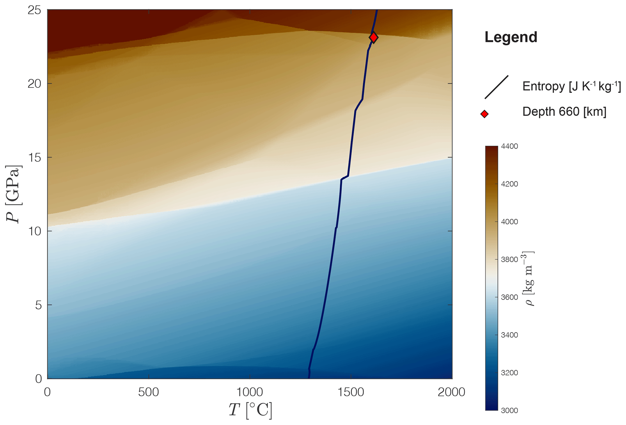
Figure A1 Hawaiian pyrolite phase diagram calculated with Perple_X (Connolly, 2005). Bulk rock composition in weight amount: 44.71 (SiO₂), 3.98 (Al2O₃), 8.18 (FeO), 38.73 (MgO), 3.17 (CaO) and 0.13 (Na₂O). Bulk rock composition taken from Workman and Hart (2005). Blue to red colours indicate density calculated for the given pressure and temperature range; the black line indicates the isentrope for a temperature of 1350 ^∘C at the base of a 120 km thick lithosphere, and the red diamond shows the pressure and temperature conditions at 660 km of depth following this isentrope.

The viscoelastic stress tensor components are defined using a backward-Euler scheme (e.g. Schmalholz et al., 2001) as

$$\begin{array}{}\text{(A4)}& {\mathit{\sigma }}_{ij}=-P{\mathit{\delta }}_{ij}+\mathrm{2}{\mathit{\eta }}^{\mathrm{eff}}{\dot{\mathit{\epsilon }}}_{ij}^{\mathrm{eff}}+J_{ij},\end{array}$$

where δ_ij=0 if i≠j, or δ_ij=1 if i=j; η^eff is the effective viscosity, and ${\dot{\mathit{\epsilon }}}_{ij}^{\mathrm{eff}}$ represents the components of the effective deviatoric strain rate tensor,

$$\begin{array}{}\text{(A5)}& {\dot{\mathit{\epsilon }}}_{ij}^{\mathrm{eff}}=({\dot{\mathit{\epsilon }}}_{ij}+{\displaystyle \frac{{\mathit{\tau }}_{ij}^o}{\mathrm{2}G\mathrm{\Delta }t}}),\end{array}$$

where G is shear modulus, Δt is the time step, ${\mathit{\tau }}_{ij}^o$ represents the deviatoric stress tensor components of the preceding time step and J_ij comprises components of the Jaumann stress rate as described in detail in Beuchert and Podladchikov (2010). A visco–elasto–plastic Maxwell model is used to describe the rheology, implying that the components of the deviatoric strain rate tensor ${\dot{\mathit{\epsilon }}}_{ij}$ are additively decomposed into contributions from the viscous (dislocation, diffusion and Peierls creep), elastic and brittle–plastic deformation as

$$\begin{array}{}\text{(A6)}& {\dot{\mathit{\epsilon }}}_{ij}={\dot{\mathit{\epsilon }}}_{ij}^{\mathrm{ela}}+{\dot{\mathit{\epsilon }}}_{ij}^{\mathrm{dis}}+{\dot{\mathit{\epsilon }}}_{ij}^{\mathrm{dif}}+{\dot{\mathit{\epsilon }}}_{ij}^{\mathrm{pei}}+{\dot{\mathit{\epsilon }}}_{ij}^{\mathrm{pla}}.\end{array}$$

In the case that deformation is effectively viscoelastic, a local iteration cycle is performed on each cell and/or node until Eq. (A6) is satisfied (e.g. Popov and Sobolev, 2008). The viscosity for the dislocation and Peierls creep flow law is a function of the second invariant of the respective strain rate components ${\dot{\mathit{\epsilon }}}_{\mathrm{II}}^{\mathrm{dis},\mathrm{pei}}={\mathit{\tau }}_{\mathrm{II}}/\left(\mathrm{2}{\mathit{\eta }}^{\mathrm{dis},\mathrm{pei}}\right)$,

$$\begin{array}{}\text{(A7)}& {\mathit{\eta }}^{\mathrm{dis}}={\displaystyle \frac{{\mathrm{2}}^{\frac{\mathrm{1}-n}{n}}}{{\mathrm{3}}^{\frac{\mathrm{1}+n}{\mathrm{2}n}}}}{A}^{-\frac{\mathrm{1}}{n}}\left({\dot{\mathit{\epsilon }}}_{\mathrm{II}}^{\mathrm{dis}}{)}^{\frac{\mathrm{1}}{n}-\mathrm{1}}\exp \right({\displaystyle \frac{Q+PV}{nRT}}\left)\right(f_{{\mathrm{H}}_{\mathrm{2}}\mathrm{O}}{)}^{-\frac{r}{n}},\end{array}$$

where the ratio in front of the prefactor A results from conversion of the experimentally derived 1D flow law, obtained from laboratory experiments, to a flow law for tensor components (e.g. Schmalholz and Fletcher, 2011). For the mantle material diffusion creep is taken into account and its viscosity takes the following form:

$$\begin{array}{}\text{(A8)}& {\mathit{\eta }}^{\mathrm{dif}}={\displaystyle \frac{\mathrm{1}}{\mathrm{3}}}{A}^{-\mathrm{1}}{d}^m\exp \left({\displaystyle \frac{Q+PV}{RT}}\right)(f_{{\mathrm{H}}_{\mathrm{2}}\mathrm{O}}{)}^{-r},\end{array}$$

where d is grain size and m is a grain size exponent. Effective Peierls viscosity is calculated using the regularized form of Kameyama et al. (1999) for the experimentally derived flow law by Goetze and Evans (1979) as

$$\begin{array}{}\text{(A9)}& {\mathit{\eta }}^{\mathrm{pei}}={\displaystyle \frac{{\mathrm{2}}^{\frac{\mathrm{1}-s}{s}}}{{\mathrm{3}}^{\frac{\mathrm{1}+\mathit{\text{s}}}{\mathrm{2}s}}}}\widehat{A}({\dot{\mathit{\epsilon }}}_{\mathrm{II}}^{\mathrm{pei}}{)}^{\frac{\mathrm{1}}{s}-\mathrm{1}},\end{array}$$

where s is an effective temperature-dependent stress exponent:

$$\begin{array}{}\text{(A10)}& s=\mathrm{2}\mathit{\gamma }{\displaystyle \frac{Q}{RT}}(\mathrm{1}-\mathit{\gamma }).\end{array}$$

$\widehat{A}$ in Eq. (A9) is

$$\begin{array}{}\text{(A11)}& \widehat{A}=\left[A\exp \right(-{\displaystyle \frac{Q(\mathrm{1}-\mathit{\gamma }{)}^{\mathrm{2}}}{RT}}){]}^{-\frac{\mathrm{1}}{s}}\mathit{\gamma }{\mathit{\sigma }}_{\mathrm{P}},\end{array}$$

where A_P is a prefactor, γ is a fitting parameter and σ_P is a characteristic stress value. The parameters A, Q, V, m and r are defined independently for each deformation mechanism (e.g. A^dis, A^dif, A^pei). However, for practical reasons we omit the corresponding superscripts (dis, dif, pei) for these material parameters.

In the frictional domain, stresses are limited by the Drucker–Prager yield function:

$$\begin{array}{}\text{(A12)}& F={\mathit{\tau }}_{\mathrm{II}}-P\sin \mathit{\varphi }-C\cos \mathit{\varphi },\end{array}$$

where ϕ is the internal angle of friction and C is the cohesion. If the yield condition is met (F≥0), the equivalent plastic viscosity is computed as

$$\begin{array}{}\text{(A13)}& {\mathit{\eta }}^{\mathrm{pla}}={\displaystyle \frac{P\sin \mathit{\varphi }+C\cos \mathit{\varphi }}{\mathrm{2}{\dot{\mathit{\epsilon }}}_{\mathrm{II}}^{\mathrm{eff}}}},\end{array}$$

and the effective deviatoric strain rate is equal to the plastic contribution of the deviatoric strain rate (Eq. A5). At the end of the iteration cycle, the effective viscosity in Eq. (A4) is either computed as the inverse of the quasi-harmonic average of the viscoelastic contributions,

$$\begin{array}{}\text{(A14)}& {\mathit{\eta }}^{\mathrm{eff}}=\left\{\begin{array}{ll}{\left(\frac{\mathrm{1}}{G\mathrm{\Delta }t}+\frac{\mathrm{1}}{{\mathit{\eta }}^{\mathrm{dis}}}+\frac{\mathrm{1}}{{\mathit{\eta }}^{\mathrm{dif}}}+\frac{\mathrm{1}}{{\mathit{\eta }}^{\mathrm{pei}}}\right)}^{-\mathrm{1}},& F<\mathrm{0}\\ {\mathit{\eta }}^{\mathrm{pla}},& F\ge \mathrm{0},\end{array}\right.\end{array}$$

or is equal to the viscosity η^pla calculated at the yield stress according to Eq. (A13). Thermal evolution of the model is calculated with the heat transfer equation:

$$\begin{array}{}\text{(A15)}& \mathit{\rho }{c}_{\mathrm{P}}{\displaystyle \frac{\mathrm{D}T}{\mathrm{D}t}}={\displaystyle \frac{\partial }{\partial x_i}}\left(k{\displaystyle \frac{\partial T}{\partial x_i}}\right)+H_{\mathrm{A}}+H_{\mathrm{D}}+H_{\mathrm{R}},\end{array}$$

where c_P is the specific heat capacity at constant pressure, D∕Dt is the material time derivative, k is thermal conductivity, H_A=Tαv_zgρ is a heat source or sink resulting from adiabatic processes assuming lithostatic pressure conditions, $H_{\mathrm{D}}={\mathit{\tau }}_{ij}({\dot{\mathit{\epsilon }}}_{ij}-{\dot{\mathit{\epsilon }}}_{ij}^{\mathrm{ela}})$ results from the conversion of dissipative work into heat (so-called shear heating), and H_R is a radiogenic heat source.

To initiate the deformation, we perturbed the initial marker field with a random amplitude vertical displacement with

$$\begin{array}{}\text{(A16)}& z_{\mathrm{M}}=z_{\mathrm{M}}+A\exp (-{\displaystyle \frac{x_{\mathrm{M}}}{\mathit{\lambda }}}),\end{array}$$

where z_M is the vertical marker coordinate in kilometres, A is a random amplitude varying between −1.25 and 1.25 km, x_M is the horizontal marker coordinate in kilometres, and λ=25 km is the half-width of the curve. The perturbation is applied to the horizontal centre of the domain between −75 and 75 km.

All physical parameters are summarized in Table A1.

Table A1 Physical parameters used in the numerical simulations M1–6.

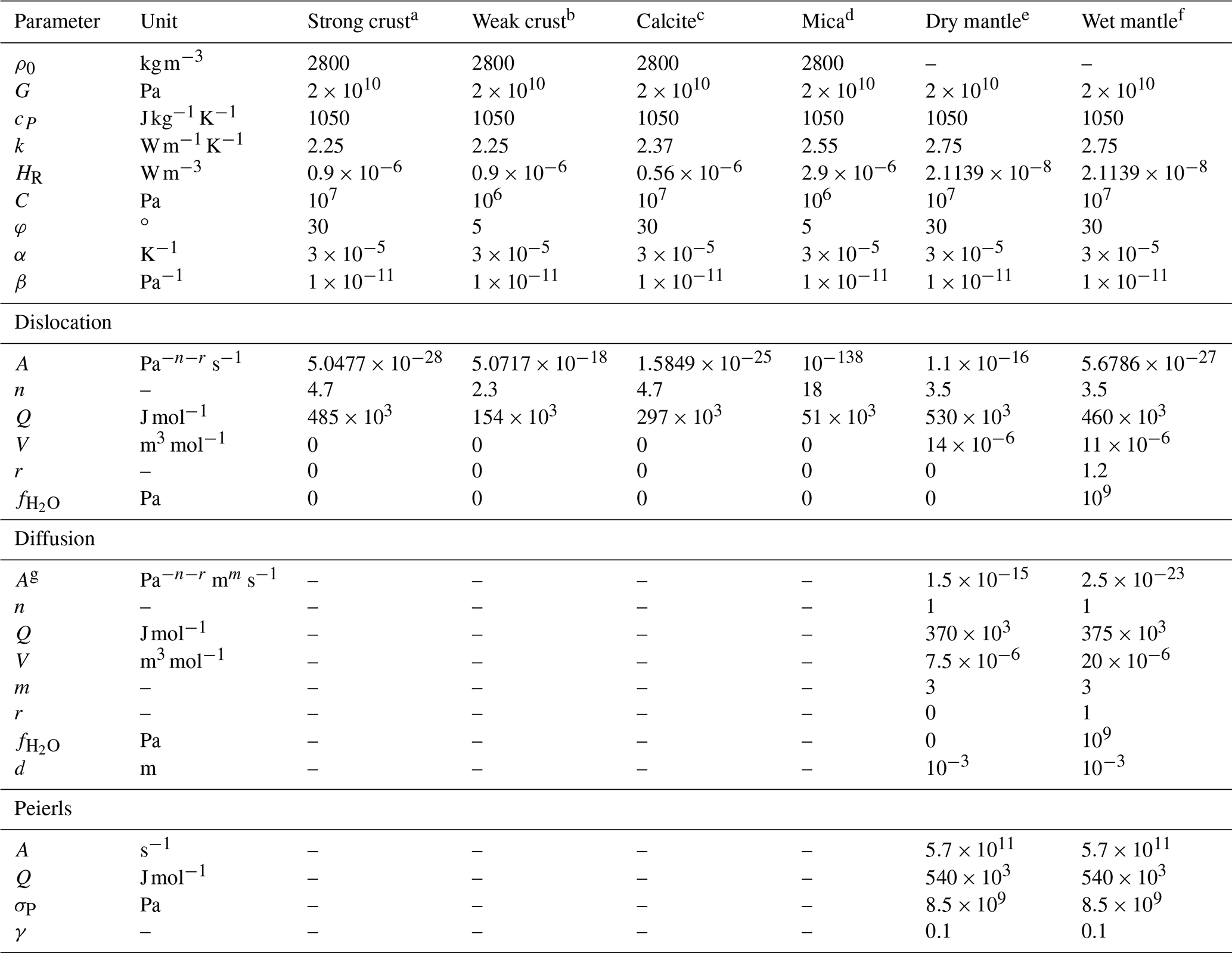
Flow law parameters: ^a Maryland diabase (Mackwell et al., 1998); ^b wet quartzite (Ranalli, 1995); ^c calcite (Schmid et al., 1977); ^d mica (Kronenberg et al., 1990); ^e dry olivine (Hirth and Kohlstedt, 2003); and ^f wet olivine (Hirth and Kohlstedt, 2003). Peierls creep: Goetze and Evans (1979) regularized by Kameyama et al. (1999). ^g Converted to SI units from original units: $A=\mathrm{2.5}\times {\mathrm{10}}^{\mathrm{7}}{\left(\left[\mathrm{MPa}\right]\right)}^{-n-r}{\left(\left[\mathrm{\mu }\mathrm{m}\right]\right)}^m{\left(\left[\mathrm{s}\right]\right)}^{-\mathrm{1}}=\mathrm{2.5}\times {\mathrm{10}}^{\mathrm{7}}\times \left({\mathrm{10}}^{-\mathrm{6}n-\mathrm{6}r}{\left[\mathrm{Pa}\right]}^{-\mathrm{6}n-\mathrm{6}r}\right)\times \left({\mathrm{10}}^{-\mathrm{6}m}[\mathrm{m}{]}^m\right)\times \left([s{]}^{-\mathrm{1}}\right)=\mathrm{2.5}\times {\mathrm{10}}^{-\mathrm{23}}\left[{\mathrm{Pa}}^{-\mathrm{2}}{\mathrm{m}}^{\mathrm{3}}{\mathrm{s}}^{-\mathrm{1}}\right]$.

Appendix B: Nusselt number scaling laws and phase transitions

Modelling thermal convection beneath an actively deforming lithosphere can be numerically expensive because the convection velocities can be as high as or even higher than the motion of the lithospheric plates, depending on the vigour of the convecting system. This significantly reduces the maximum time step necessary to ensure numerical stability. In consequence, it takes more time steps to run a simulation to the same physical time when convection is modelled together with deformation in the lithosphere. Hence, the computational time can be twice as long compared to models with which only the deforming lithosphere is modelled. However, it is possible to include the effect of convection in the mantle on the thermal field and keep a constant vertical heat flux through the lithosphere–asthenosphere boundary (LAB) into a numerical model without explicitly modelling convection by using an effective thermal conductivity for the mantle material below the lithosphere. Two dimensionless quantities have to be defined, namely the Rayleigh and Nusselt numbers. The Rayleigh number is the ratio of the thermal diffusion and advection timescale:

$$\begin{array}{}\text{(B1)}& \mathit{Ra}={\displaystyle \frac{t_{\mathrm{Dif}}}{t_{\mathrm{Adv}}}}={\displaystyle \frac{\mathit{\rho }g\mathit{\alpha }\mathrm{\Delta }T{D}^{\mathrm{3}}}{\mathit{\kappa }{\mathit{\eta }}_{\mathrm{eff}}}},\end{array}$$

where ρ is density, g is gravitational acceleration, α is a coefficient of thermal expansion, ΔT is the temperature difference between the top and the bottom, and D is the thickness of the convecting layer; $\mathit{\kappa }=k/\mathit{\rho }/c_P$ is the thermal diffusivity, and η_eff is the effective viscosity. The Nusselt number can be expressed in terms of the Rayleigh number as

$$\begin{array}{}\text{(B2)}& \mathit{Nu}=({\displaystyle \frac{\mathit{Ra}}{{\mathit{Ra}}_{\mathrm{crit}}}}{)}^{\mathit{\beta }},\end{array}$$

where Ra_crit is the critical Rayleigh number at which convection starts, typically of the order of 10³, and β is a power-law exponent (Schubert et al., 2001). The Nusselt number is the ratio of advective heat flux, q_Adv, which is the vertical heat flux through the base of the lithosphere imposed by the convecting upper mantle to the diffusive heat flux, q_Dif, imposed by the lithosphere on top of the convecting upper mantle as

$$\begin{array}{}\text{(B3)}& \mathit{Nu}={\displaystyle \frac{q_{\mathrm{Adv}}}{q_{\mathrm{Dif}}}}.\end{array}$$

Using this relationship, it is possible to scale the thermal conductivity to the Nusselt number of the Earth's mantle and to maintain a constant heat flow through the base of the lithosphere via conduction when convection is absent. Assuming $\mathit{Ra}=\mathrm{2}\times {\mathrm{10}}^{\mathrm{6}}$ and $\mathit{\beta }=\mathrm{1}/\mathrm{3}$ for the Earth's upper mantle convection, Eq. (B2) predicts Nu=13. This implies that the heat flow provided by advection is 13 times higher than the heat flow provided by conduction. Using an effective conductivity approach, the heat flow provided by advection is mimicked using an enhanced conductive heat flow in the upper mantle. The effective conductivity can be determined by scaling the standard value of thermal conductivity of the upper mantle material to the Nusselt number of the convecting system with

$$\begin{array}{}\text{(B4)}& k_{\mathrm{eff}}=\mathit{Nu}k.\end{array}$$

For this study, the standard value is k=2.75 for the upper mantle material and Nu=13. The effective conductivity according to Eq. (B4) is k_eff=36. To avoid a strong contrast of conductivities directly at the base of the lithosphere, we linearly increase the conductivity from 2.75 to 36 W m⁻¹ K⁻¹ over a temperature range of 1350–1376 ^∘C. Applying this effective conductivity approach reduces the number of time steps necessary for computation up to the same physical time by approximately a factor 2 in M4 compared to M1.

As mentioned above, the vigour of convection is defined by the Rayleigh number (Eq. B1). For Ra≫Ra_crit, the timescale for thermal diffusion is much larger than the timescale for advection of material. This means that the entropy of the system remains relatively constant in time. By definition, such a system is adiabatic (Kondepudi and Prigogine, 2014). In the presented models, the density and entropy for the mantle phases are pre-computed using Perple_X for a given bulk rock composition. Assuming that the temperature gradient in the upper mantle is adiabatic and stress conditions are close to lithostatic (i.e. deviatoric stresses are negligible), the temperature at any depth can be determined by following an isentrope from the Perple_X database. Starting coordinates in pressure–temperature space are the (lithostatic) conditions at the base of the lithosphere. From these pressure and temperature values one can follow the closest isentrope (black line Fig. A1) until the (lithostatic) pressure value at the target depth (in this study 660 km, red diamond Fig. A1) is reached and extract the corresponding temperature value. Trubitsyn and Trubitsyna (2015) derived an analytical solution to calculate temperatures assuming an adiabatic gradient for given depths. We determined the temperature at the bottom of the model domain using both approaches and the obtained values that differ by only 0.01 ^∘C.

Involving phase transitions necessitates mainly two major assumptions: (1) is compressibility of material due to large density variations important? (2) Does latent heat released or consumed at a phase transition significantly change the convective pattern? Bercovici et al. (1992) concluded that compressibility effects on the spatial structure of mantle convection are minor when the superadiabatic temperature drop is close to the adiabatic temperature of the mantle, which is the case for the Earth. Although the net density varies largely in P−T space of the phase diagram used in this study (Fig. A1), the maximum value for the density time derivative computed from M1 is 2 orders of magnitude lower than the velocity divergence. We assume that density changes due to volumetric deformation are hence still negligible and density changes are accounted for in the buoyancy force only. This means the classical Boussinesq approximation is still valid. However, not considering adiabatic heating in the energy conservation equation leads to a significant deviation of the thermal structure from the initially imposed temperature gradient over large timescales (>100 Myr). The resulting temperature profile is constant throughout the upper mantle, and the newly equilibrated constant temperature is equal to the imposed temperature at the bottom boundary. In consequence, the density structure read in from the phase diagram table according to pressure and temperature values is significantly wrong. To avoid these problems, we use the extended Boussinesq approximation; i.e. the adiabatic heating term is included in the energy conservation equation. As a result, the initially imposed adiabatic (or isentropic) temperature gradient can be maintained over large timescales. The resulting density structure agrees well with the PREM (Dziewonski and Anderson, 1981) as shown in this study. A detailed comparison between different approximations of the system of equations is clearly beyond the scope of this study.

Latent heat that is released or consumed by a phase transition can perturb the thermal field by up to 100 K and induce a buoyancy force aiding or inhibiting the motion of cold, especially low-angle, subducting slabs (van Hunen et al., 2001) or hot rising plumes. However, when the lateral differences in temperature are small, the deflection of the phase transition by an ascending plume or a subducting slab has a much bigger impact on the buoyancy stresses than the latent heat released or consumed by the phase transition (Christensen, 1995). Because a detailed parametric investigation of the impact of latent heat on buoyancy stresses is beyond the scope of study, we neglect latent heat for simplicity.

Appendix C: Convection benchmark

In this section, we present the results of a convection benchmark performed by the algorithm used in this study. Equations for continuity and force balance are solved as in Eqs. (A2) and (A1), and density is a function of temperature only calculated as

$$\begin{array}{}\text{(C1)}& \mathit{\rho }\left(T\right)={\mathit{\rho }}_{\mathrm{0}}(\mathrm{1}-\mathit{\alpha }T).\end{array}$$

The total stress tensor is decomposed into a pressure and a deviatoric part as

$$\begin{array}{}\text{(C2)}& {\mathit{\sigma }}_{ij}=-P{\mathit{\delta }}_{ij}+{\mathit{\tau }}_{ij}.\end{array}$$

Transfer of heat is calculated as in Eq. (A15). Stresses and strain rates (${\dot{\mathit{\epsilon }}}_{ij}$) are related to each other via the viscosity η as

$$\begin{array}{}\text{(C3)}& {\mathit{\tau }}_{ij}=\mathrm{2}\mathit{\eta }{\dot{\mathit{\epsilon }}}_{ij}.\end{array}$$

Viscosity is computed via a linearized Arrhenius law, also called the Frank-Kamenetskii approximation (Kamenetskii, 1969):

$$\begin{array}{}\text{(C4)}& \mathit{\eta }(T,z)=\exp (-{\mathit{\gamma }}_T+{\mathit{\gamma }}_z),\end{array}$$

with γ_T=log (η_T) and γ_z=log (η_z). By choosing η_z=1, γ_z=0 in Eq. (C4), and therefore the viscosity is only temperature-dependent.

The dimensionless equations are discretized over a domain that extends from 0 to 1 in both horizontal and vertical directions, and a small amplitude perturbation (A=0.01) is applied to the initial temperature profile as

$$\begin{array}{}\text{(C5)}& T(x,\mathit{\text{z}})=(\mathrm{1}-z)+A\cos \left(\mathit{\pi }x\right)\sin \left(\mathit{\pi }z\right).\end{array}$$

As mentioned above, the vigour of the convecting system is described by its Rayleigh number (Eq. B1). A local Ra=10² is applied to the top boundary by setting $\mathit{\alpha }={\mathrm{10}}^{-\mathrm{2}}$ and g=10⁴, and all other parameters of Eq. (B1) are set to 1. The applied viscosity decrease by choosing η_T=10⁵ in Eq. (C4) results in a global Ra=10⁷. All mechanical boundaries are set to free slip; the thermal boundary conditions are constant temperature at the top (T=0) and bottom (T=1) and insulating (i.e. zero flux) at the two vertical boundaries. Tosi et al. (2015) tested several algorithms, including finite element, finite differences, finite volume and spectral discretization, on their capability of modelling distinct rheologies of the mantle from temperature-dependent viscosity only up to visco-plastic rheologies. We have chosen the simplest test, case one in Tosi et al. (2015), and report the results of two distinct diagnostic quantities: the average temperature over the entire modelling domain,

$$\begin{array}{}\text{(C6)}& \langle T\rangle =\underset{\mathrm{0}}{\overset{\mathrm{1}}{\int }}\underset{\mathrm{0}}{\overset{\mathrm{1}}{\int }}T\mathrm{d}x\mathrm{d}z,\end{array}$$

and the root mean square velocity at the surface

$$\begin{array}{}\text{(C7)}& u_{\mathrm{RMS}}^{\mathrm{surf}}=(\underset{\mathrm{0}}{\overset{\mathrm{1}}{\int }}{v}_x^{\mathrm{2}}{|}_{z=\mathrm{1}}\mathrm{d}x{)}^{\frac{\mathrm{1}}{\mathrm{2}}}.\end{array}$$

The model develops one convection cell below a stagnant lid (Fig. C1a). We tested numerical resolutions of 50², 100², 150² and 300². Only for resolutions >100² did the desired convective pattern develop. The numerical algorithms tested by Tosi et al. (2015) passed the benchmark for lower resolutions. This is due to the fact that the algorithm presented here uses a uniform grid size across the domain. The algorithms tested by Tosi et al. (2015) used refined meshes. Sufficient resolution of the thermal boundary layers at the top and at the bottom is crucial to develop the desired pattern. Using a refined mesh in these regions allows for lower total resolution, whereas using a regular mesh necessitates a much higher resolution in total. Nevertheless, values for the diagnostic quantities reproduced by the presented algorithm lie well within the minimum and maximum values calculated by the algorithms tested in Tosi et al. (2015) (grey areas in Fig. C1b, d). This shows that the convection in the upper mantle, where the viscosity is essentially temperature-dependent, in the models presented in this study for which convection is not parameterized is accurately modelled.

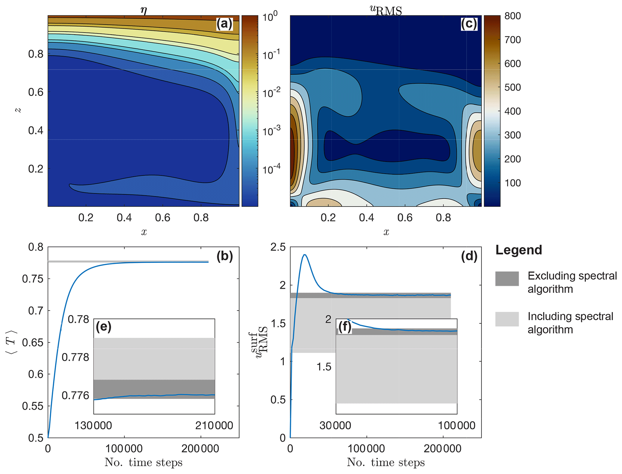
Figure C1 Results of 2D convection benchmark. (a) Effective viscosity after convection reached a steady state, (b) normal average temperature calculated as in Eq. (C6) for the entire model history, (c) root mean square velocity field for the entire domain after convection reached a steady state, (d) root mean square velocity at the surface of the modelled domain of the entire model history calculated as in Eq. (C7), (e) normal average temperature calculated as in Eq. (C6) for the time period at which the convection reaches a steady state and (f) root mean square velocity at the surface of the modelled domain calculated as in Eq. (C7) for the time period at which the convection reaches a steady state. In Fig. C1b and C1d–f, the dark grey area only shows the range of minimum and maximum values for the given diagnostic quantity obtained by the algorithms tested by Tosi et al. (2015) excluding the spectral algorithm. Dark combined with light grey areas indicate the range obtained by all algorithms tested by Tosi et al. (2015) including the spectral algorithm.

Appendix D: Gravitational potential energy and plate driving forces

We use the gravitational potential energy (GPE) per unit surface to quantify the impact of convection-induced density variations in the upper mantle during the distinct stages of the simulations. The GPE varies along the horizontal x direction and is computed as

$$\begin{array}{}\text{(D1)}& \text{GPE}\left(x\right)=\underset{\mathrm{Sb}}{\overset{\mathrm{St}\left(x\right)}{\int }}{P}_{\mathrm{L}}(x,z)\mathrm{d}z,\end{array}$$

where P_L is the lithostatic pressure calculated as

$$\begin{array}{}\text{(D2)}& P_{\mathrm{L}}(x,z)=\underset{z}{\overset{\mathrm{St}\left(x\right)}{\int }}\mathit{\rho }(x,z^{\prime })g\mathrm{d}{z}^{\prime },\end{array}$$

where St(x) is the stress-free surface and Sb is the model bottom. Horizontal variations in GPE, ΔGPE, are calculated by subtracting the leftmost value as a reference value from all other values. The GPE gives an estimate of the plate driving forces per unit length (Molnar and Lyon-Caen, 1988; Schmalholz et al., 2019; Bessat et al., 2020) acting in the system during the different stages of the hyperextension and convergence cycle. We also calculate the vertical integral of the second invariant of the deviatoric stress tensor:

$$\begin{array}{}\text{(D3)}& {\stackrel{\mathrm{‾}}{\mathit{\tau }}}_{\mathrm{II}}\left(x\right)=\underset{\mathrm{Sb}}{\overset{\mathrm{St}\left(x\right)}{\int }}{\mathit{\tau }}_{\mathrm{II}}(x,z)\mathrm{d}z.\end{array}$$

The value of $F_{\mathrm{D}}=\mathrm{2}\times {\stackrel{\mathrm{‾}}{\mathit{\tau }}}_{\mathrm{II}}^{\mathrm{avg}}\left(x\right)$, where ${\stackrel{\mathrm{‾}}{\mathit{\tau }}}_{\mathrm{II}}^{\mathrm{avg}}\left(x\right)$ is calculated by averaging ${\stackrel{\mathrm{‾}}{\mathit{\tau }}}_{\mathrm{II}}\left(x\right)$ over both the leftmost and rightmost 100 km of the domain, is also identical to the vertical integral of the difference between the horizontal total stress and the lithostatic pressure if shear stresses are negligible (Molnar and Lyon-Caen, 1988; Schmalholz et al., 2019). This condition is strictly satisfied by the choice of boundary conditions at the top and the bottom of the model domain. We therefore chose to show the profiles which have been integrated over the entire domain height ($z=-\mathrm{660}$ km). Since the deviatoric stresses below the lithosphere are indeed negligibly small, values for F_D integrated from depths of $z=-\mathrm{660}$ km, $z=-\mathrm{330}$ km and $z=-\mathrm{120}$ km do not reveal significant differences. Therefore, the value of F_D is essentially independent of the integration depth (if deeper than the lithosphere thickness). F_D can therefore be used to estimate the plate driving force (see Fig. 7d). For calculation of the suction force per unit length (F_S) induced by the mantle flow (Fig. 6a, f) we used the following formula:

$$\begin{array}{}\text{(D4)}& F_{\mathrm{S}}=\underset{b}{\overset{a}{\int }}\underset{d}{\overset{c}{\int }}\mathrm{\Delta }\mathit{\rho }g\mathrm{d}z\mathrm{d}x,\end{array}$$

where a, b, c and d are the integration bounds, and Δρ is the difference in density between the entire density field at the end of the cooling period and a reference density value (profiles in Fig. 2e).