the Creative Commons Attribution 4.0 License.
the Creative Commons Attribution 4.0 License.
 | 23 Dec 2020
Seismic gaps and intraplate seismicity around Rodrigues Ridge (Indian Ocean) from time domain array analysis
Manvendra Singh
Georg Rümpker
Rodrigues Ridge connects the Réunion hotspot track with the Central Indian Ridge (CIR) and has been suggested to represent the surface expression of a sub-lithospheric flow channel. From global earthquake catalogues, the seismicity in the region has been associated mainly with events related to the fracture zones at the CIR. However, some segments of the CIR appear void of seismic events. Here, we report on the seismicity recorded at a temporary array of 10 seismic stations operating on Rodrigues Island from September 2014 to June 2016. The array analysis was performed in the time domain by time shifting and stacking the complete waveforms. Event distances were estimated based on a 1-D velocity model and the travel time differences between S and P wave arrivals. We detected and located 63 new events that were not reported by the global networks. Most of the events (51) are located off the CIR and can be classified as intraplate earthquakes. Local magnitudes varied between 1.6 and 3.7. Four seismic clusters were observed that occurred to the west of the spreading segment of the CIR. The Rodrigues Ridge appeared to be aseismic during the period of operation. The lack of seismic activity along both Rodrigues Ridge and the sections of the CIR to the east of Rodrigues may be explained by partially molten upper-mantle material, possibly in relation to the proposed material flow between the Réunion plume and the CIR.
- Article
(10441 KB) - Full-text XML
-
Supplement
(758 KB) - BibTeX
- EndNote


The theory of plate tectonics is largely supported by the occurrence of seismicity along (oceanic) ridge systems, subduction zones, and mountain belts. However, a substantial part of seismicity occurs off the ridge axes within the oceanic basins. Such events are usually denoted as intraplate earthquakes (Krishna et al., 1998; Okal, 1983). Gutenberg and Richter (1941) made the first attempt to document these intraplate events. A more systematic approach was adopted by Sykes and Sbar (1973) and later by Bergman and Solomon (1980), where they compiled a catalog of 159 oceanic intraplate events between 1939 and 1979. Assessing the seismicity inside the oceanic environment has always been a challenge as most of the permanent stations are located on the islands where the attenuation of the seismic signal along the oceanic path further reduces the detection capability. Another factor contributing to this problem is swell-generated noise in the band of 1–5 s (Okal, 1983).
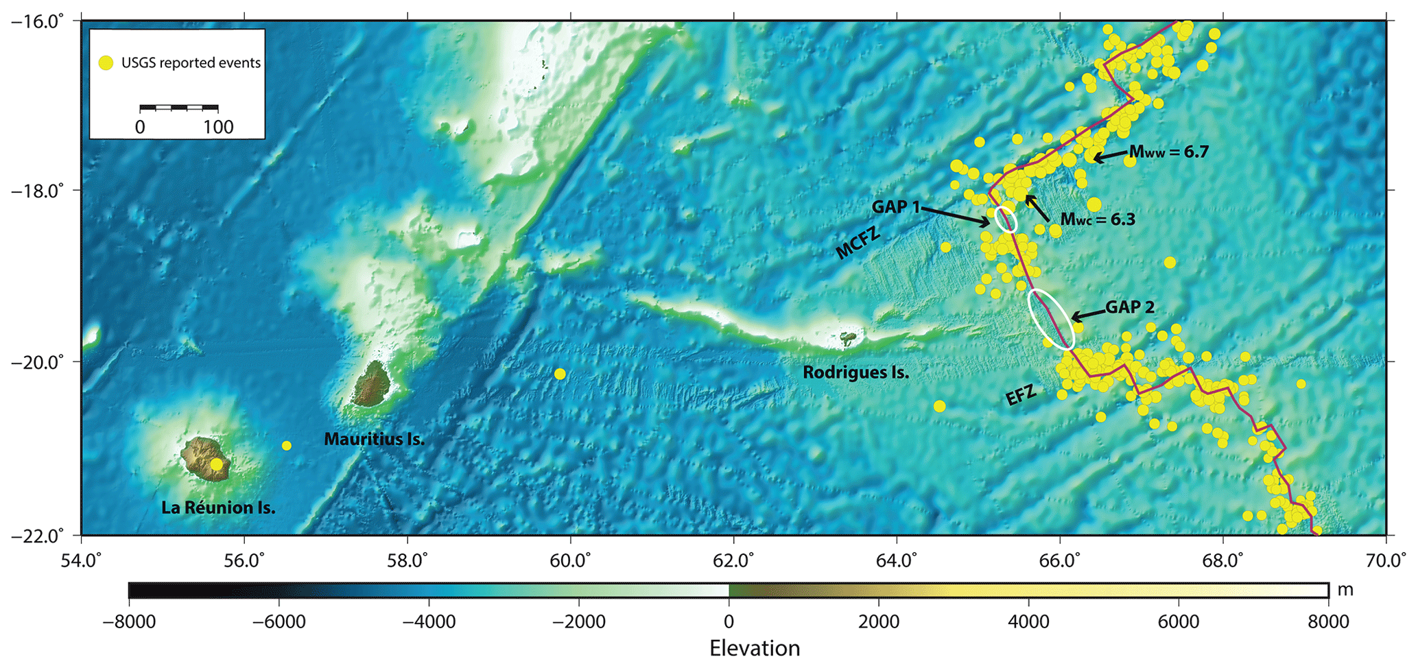
Figure 1Tectonic setting of Rodrigues Ridge–Central Indian Ridge (CIR) region. The ridge axis is shown by a solid line (red). Event locations from USGS catalogue (January 2000–August 2020) are shown in yellow. MCFZ stands for Marie-Celeste fracture zone, and EFZ stands for Egeria fracture zone. The gaps in seismicity (GAP 1 and GAP 2) along the section of CIR between MCFZ and EFZ have been marked by white ellipses.
Rodrigues Island is found at the eastern extremity of the Rodrigues Ridge near 63∘25′ E and 19∘42′ S, approximately 650 km east of Mauritius. The east–west trending Rodrigues Ridge was formed between 7 and 10 Ma (Dyment et al., 2007; Saddul et al., 2002). It is suggested that it represents the surface expression of the interaction of the Réunion Hotspot with the Central Indian Ridge (CIR) through a sublithospheric flow channel (Duncan and Hargraves, 1990; Dyment et al., 2007; Bredow et al., 2017) though Conrad and Behn (2010) and Becker and Faccenna (2011) suggest deeper mantle circulation as the possible mechanism of the formation of Rodrigues Ridge. Samples collected from several sites along the ridge suggest that it is composed of basaltic rocks (Dyment et al., 2001). As Rodrigues Island is approximately 250 km from the active southern part of CIR, seismicity around it is generally characterized by events recorded along this ridge system (Fig. 1). The largest magnitudes, 6.3 and 6.7, were recorded on 16 August 2010 and 26 July 2012, respectively, at the CIR near Rodrigues. It was also observed that earthquakes with magnitudes 6 or greater are concentrated along Marie-Celeste fracture zone (MCFZ) only. Krishna et al. (1998) reported six events between October and November 1984 near the ridge, on the east of the spreading segment, between the Egeria fracture zone (EFZ) and MCFZ. Similarly, Bergman et al. (1984) have reported a large number of “off-ridge” earthquakes in the region of the Southeast Indian Ridge. Interestingly, there are two segments along the CIR, between MCFZ and EFZ, for which the global catalogues are void of any seismicity (denoted GAP 1 and GAP 2 in Fig. 1).
In this study we use seismological array techniques (Harjes and Henger, 1973; Husebye and Ruud, 1989; Rost and Thomas, 2002) to characterize the seismic activity around the region of the Rodrigues Ridge and to confirm the seismic gaps and provide possible explanations for them. The data for this study were collected from temporary deployment of a seismic array on Rodrigues Island between September 2014 and June 2016 (Fig. 2).
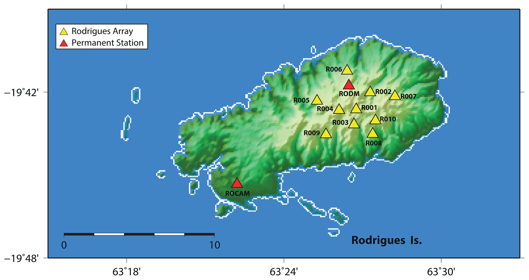
Figure 2Locations of individual stations in Rodrigues array (yellow triangles). Red triangles denote permanent stations ROCAM and RODM. Station RODM was operational between 10 November 2010 and 7 September 2014.
2.1 Array configuration
In order to study the seismicity around Rodrigues Ridge, we deployed an array of 10 seismic stations on the island of Rodrigues located at about 19∘42′ S and 63∘25′ E approximately 250 km west of the CIR. Rodrigues array design is based on classical nine-element arrays that use three and five seismic sensors located along two concentric rings, respectively, with an additional sensor placed in the center. The benefit of this configuration is that with irregular sensor spacing it provides a relatively sharp maximum of the array response function (Haubrich, 1968). For Rodrigues array, we deployed 10 sensors in a similar configuration with a ∼1.5 km radius of the inner ring and an outer ring radius of ∼2.5 km (Fig. 3). The final locations of the individual stations were then chosen according to the local conditions on the island (such as accessibility by roads, etc.). Each station consisted of a MARK L-4C-3D (1 Hz) sensor and an Omnirecs CUBE data logger recording at a sampling rate of 100 Hz.
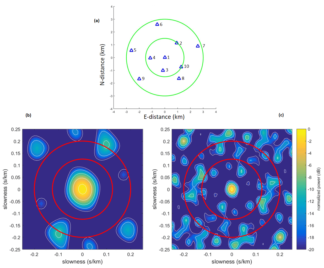
Figure 3Configuration of the seismic array deployed on Rodrigues Island (a). Station locations are indicated by blue triangles. The green circles represent inner and outer rings of the array with a radius of ∼1.5 and ∼2.5 km, respectively, from the central (reference) station. The array transfer function of the Rodrigues array is shown at 2 Hz (b) and 5 Hz (c). The inner and the outer red rings correspond to an apparent velocity of 8 and 5 km s−1, respectively. In the real-data analysis, the apparent velocity at which the maximum occurs is used as a first indication to discriminate between crustal and upper-mantle ray paths.
The relatively large aperture of the array (∼5 km) was chosen based on events listed in the USGS catalogue, which are located at the CIR near Rodrigues and were also recorded at the permanent station RODM. This GEOSCOPE station was relocated during the course of the array deployment. The dominant frequency of these events is close to about 2 Hz. However, it became clear later that the dominant frequency of most earthquakes recorded by the newly installed array is approximately 5 Hz. Therefore, we decided to perform the array analysis in the time domain, or equivalently for a wide frequency range to reduce possible ambiguities resulting from side lobes in the array response function (Fig. 3), as will be discussed further below. A similar approach was also used by Leva et al. (2019).
2.2 Epicentral distance and origin time
For regional earthquakes, the slowness (apparent velocity) cannot be used to determine the epicentral distance of an event, as the ray path is mainly confined within the uppermost mantle and the depth variations of velocity are not well constrained. We, therefore, use the arrival-time difference between the S and P waves in conjunction with a simplified 1-D velocity model of the crust and upper mantle to approximately determine the epicentral distance.
In this model, we keep the hypocentral depth fixed at 6 km, and the ray path corresponds to a head wave (Fig. 4). From receiver function analysis (Fontaine et al., 2015), a Moho depth of 10 km has been determined beneath Rodrigues Island. We fix the crustal thickness in our laterally homogeneous model to this value, such that the thickened oceanic crust is accounted for on the receiver side leg of the ray path. For the P wave velocity in the crust, we assume and in the mantle we assume with a VP∕VS ratio of 1.80, as suggested by results of Christensen (2004), Kong et al. (1992), Wolfe et al. (1995), and Grevemeyer et al. (2013). We explored the influence of these parameters on the determination of the epicentral distances for the events that occur at the distances of ∼120 and ∼265 km from the array. As shown in Figs. S1 and S2 in the Supplement, results are most sensitive to variations of the P wave velocity in the mantle and VP∕VS, owing to its contribution to the ray path.

Figure 4Cartoon depicting the model employed to estimate epicentral distances from travel-time differences between S and P wave arrival. The simple 1-D velocity model of the oceanic crust and uppermost mantle consists of a uniform layer overlying a uniform half-space. The parameters are set as follows: thickness of the crust, d=10 km; hypocentral depth, h=6 km; P wave velocity in the crust, ; P wave velocity in the mantle, ; in both the crust and mantle. Figures S1 and S2 in the Supplement show the influence of these parameters on the determination of the epicentral distance.
The final value for the epicentral distance of an event (with respect to the center of the array) is obtained by taking the mean of the distance values determined at all stations of the array. Stations for which the recordings do not exhibit a clear onset for either the P or S phase are discarded from this calculation. The standard deviation (SD) is used to define the error of the distance calculation.
To determine the event origin time, torigin, the travel time, ttt, was calculated from the distance obtained from the S and P wave travel time difference for the central (reference) station. By subtracting this value from the manually picked P wave arrival time, tP, we obtain , where it is assumed that tP is given as an absolute time value.
2.3 Magnitude determination
In order to calculate the magnitude of an event, we account for the sensitivity of the recording system (CUBE data logger and 1 Hz MARK sensor) and integrate the velocity seismogram, which is then convolved with the Wood–Anderson transfer function to obtain the ground displacement in nanometers. Magnitudes are determined based on the maximum (absolute) amplitude of the horizontal components using all available stations for which the recordings show a clear (dominant) S phase. Again, the mean and the SD of the magnitude value is calculated. As most of the events are located well within a 1000 km radius, we use the relation given by Havskov and Ottemöller (1999) in SEISAN package to determine the local magnitude
where A is the amplitude (in nm) and Δ is the epicentral distance (in km).
2.4 Beamforming and array transfer function
In seismic array analysis, the slowness and the back azimuth of an event are determined by beamforming. Assuming a plane wave front of horizontal slowness s0 moving across the array with an apparent velocity(), the waveform at station j is given by
where rj defines the position of the station with respect to a suitable coordinate system.
For an array consisting of M stations, the beam energy is calculated from the trace amplitudes within a suitable time window defined by t1 and t2 according to (e.g., Harjes and Henger, 1973; Rost and Thomas, 2002)
where s denotes the (trial) slowness for the current beam. The beam energy reaches a maximum, if s=s0. The back azimuth is then obtained from slowness components according to , where x and y correspond to the eastern and northern components, respectively (see details given below).
In view of Eq. (1) and using Parseval's theorem in combination with the shift theorem of Fourier transforms, we can write the energy in the form
where the bar denotes Fourier-transformed functions and the array transfer function, , in the frequency–slowness domain is given by (e.g., Schweitzer, 2002)
It is further assumed that is outside of the range of integration used in Eq. (4). The array transfer function defines the sensitivity and resolution of the array for seismic signals with frequency ω (Fig. 3).
2.5 Data example
All the events for this study were detected by manual inspection of hourly traces from all stations of the Rodrigues array using the SEISAN package (Havskov and Ottemöller, 1999). A time window of 120 s was cut around each event using the GIPPtool software (http://www.gfz-potsdam.de, last access: August 2019).
As shown in Fig. 5, we estimate the epicentral distance from the arrival-time differences of the S and P waves. The STA ∕ LTA ratio of the Z-component trace is calculated to aid in the manual picking of the two arrivals. All S picks were made independently and are based on visual inspection of horizontal components as well as vertical components where necessary. The mean of the P phase picking time, calculated from all the picks, is used to determine the time window to calculate the beam energy later in the array analysis. For this example, the arrival-time difference is 13.3 s, which corresponds to a distance of approximately 119 km (Table S1). Finally, the magnitude of the event is calculated from Eq. (1). Here, we obtain a magnitude of 3.0. In the following, we apply this methodology to all events detected that exhibit a clear P and S wave onset.
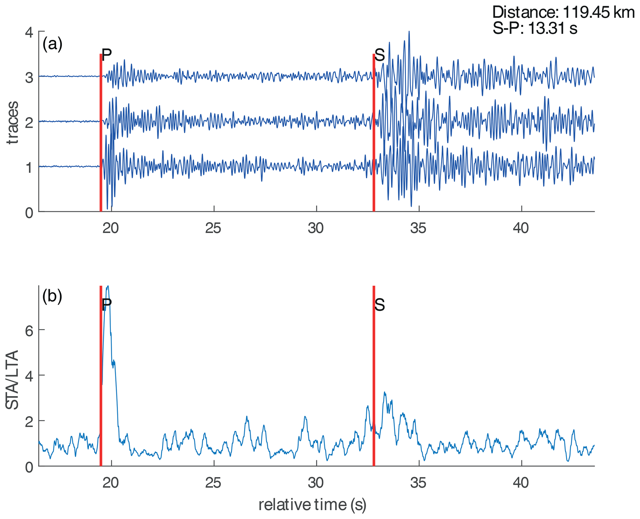
Figure 5Estimating the epicentral distance from the arrival-time difference between S and P waves at the reference station 1. The vertical, north, and east components are shown by traces 1, 2, and 3, respectively (a). The vertical red lines show manually picked P and S phases. The picking is aided by calculating the STA ∕ LTA of the Z component (b).
Conventionally, array analyses are performed in the frequency domain, which is computationally advantageous as the energy stacking can be limited to the dominant frequency or a narrow frequency band. As explained above, however, we perform the array analysis in the time domain to include the complete waveform of the first arrival. The time domain analysis corresponds to a broadband energy stack and suppresses the effects of unwanted side lobes, but there is an additional benefit: the frequency domain approach usually requires selection of a common time window for all traces before the Fourier transform is applied. In cases of significantly different arrival times of the phase to be analyzed (e.g., due to a large aperture of the array), a relatively wide common time window has to be selected such that the cut waveforms of individual traces may be significantly different. In the time domain, however, we can time shift the traces (with respect to the trial slowness value) before cutting and stacking, which may then be performed within a much narrower time window. This approach ensures that only the relevant waveform is contained within the stack, provided that the correct time shift has been applied.
Our analysis involves applying time shifts to all the traces with respect to reference trace (no. 1) for different values of slowness, defined by a grid, and calculating the energy of the resulting stacked trace or beam within the time window of the first arrival, which is selected using mean of the P wave picks on all the usable traces for a given earthquake. Only vertical (Z) component traces from all stations were used for the beamforming.
Figure 6a shows the Z component traces for an earthquake on 6 April 2015 originating at 20:25:42 UTC. A band pass between 2 and 10 Hz is applied. The trace number on the vertical axis corresponds to the respective station number. The amplitudes of trace 3 are set to zero as it did not show a clear event.
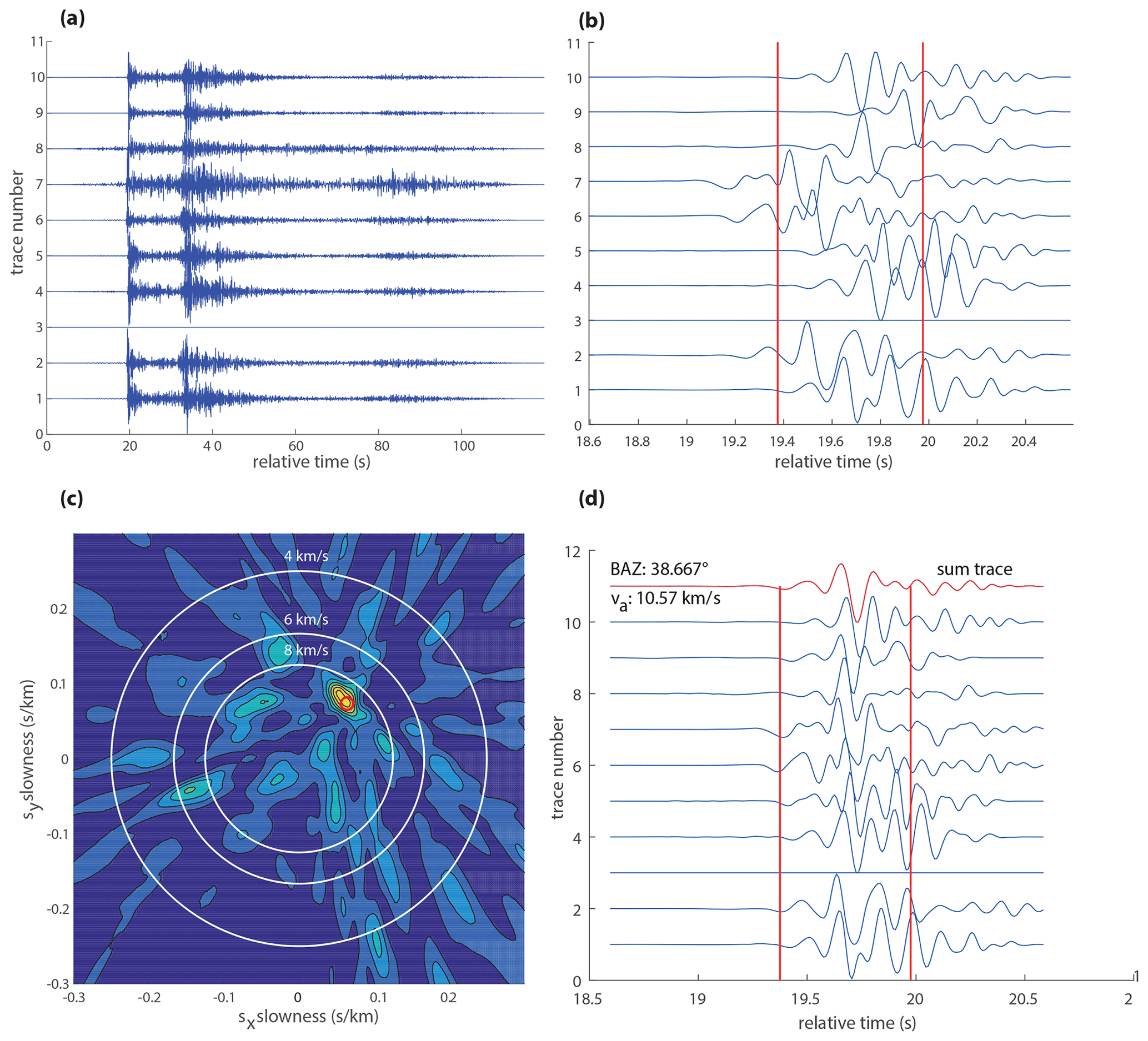
Figure 6Array analysis of a regional event near Rodrigues. (a) Vertical-component traces. Station 3 was not recording at the time of the event. (b) Zoom-in of the P waveforms. After applying the time shift corresponding to a trial slowness s, the beam energy is calculated from squared amplitudes within the time window enclosed by the red circle. (c) Beam energy as function of horizontal slowness components sx and sy. The maximum is marked by a red line and corresponds to the slowness s0. White circles denote apparent velocities, va, of 4, 6, and 8 km s−1. (d) Shifted traces and beam (red trace) corresponding to the maximum indicated in (c). The back azimuth of this event is determined at about 38∘ with an apparent velocity of 10.57 km s−1.
At first, a relatively wide time window (∼2 s) is automatically chosen to zoom-in on the P phase (Fig. 6b). Then, a narrower time window (∼0.6 s or about three dominant periods wide, as indicated by the red vertical lines) is automatically selected with respect to reference trace 1 based on the P phase picking on all the traces. Time shifts are applied to all other (normalized) traces in correspondence to the slowness values of the grid which is used in the energy stack (Fig. 6c). The stack, however, is only calculated from the trace segments within the narrow time window.
A predefined grid with slowness from −0.3 to 0.3 s km−1, equally spaced over points is used for calculating the appropriate time shifts for each trace and the resulting energy. The red circle in Fig. 6c denotes the maximum beam energy at s km−1, which corresponds to a back azimuth and . We assume that this relatively large value for the apparent velocity results from steepening of the ray path at shallow depth beneath Rodrigues Island (where the propagation velocity is smaller than 6.1 km). The corresponding shifted traces and the beam (by summing the amplitudes of all traces) are shown in Fig. 6d.
The values of slowness components thus obtained, were used to calculate the corresponding apparent velocity, va and the back azimuth, Φ of the event according to
where s0x and s0y are the values of slowness vector obtained for the beam with maximum energy.
To estimate the error in back azimuth, δΦ, we define the area enclosed by the contour at a level of 95% of the maximum beam energy as a confidence region. The error in back azimuth in terms of kilometers (δΦkm) is then given by
where Δ is the epicentral distance (in km) and δΦ is given in degrees.

Figure 7Estimating the epicentral distance from the arrival-time difference between S and P waves at reference station 1. The vertical, north, and east components are shown by traces 1, 2, and 3, respectively (a). The vertical red lines show manually picked P and S phases. The picking is aided by calculating the STA ∕ LTA of the Z component (b).
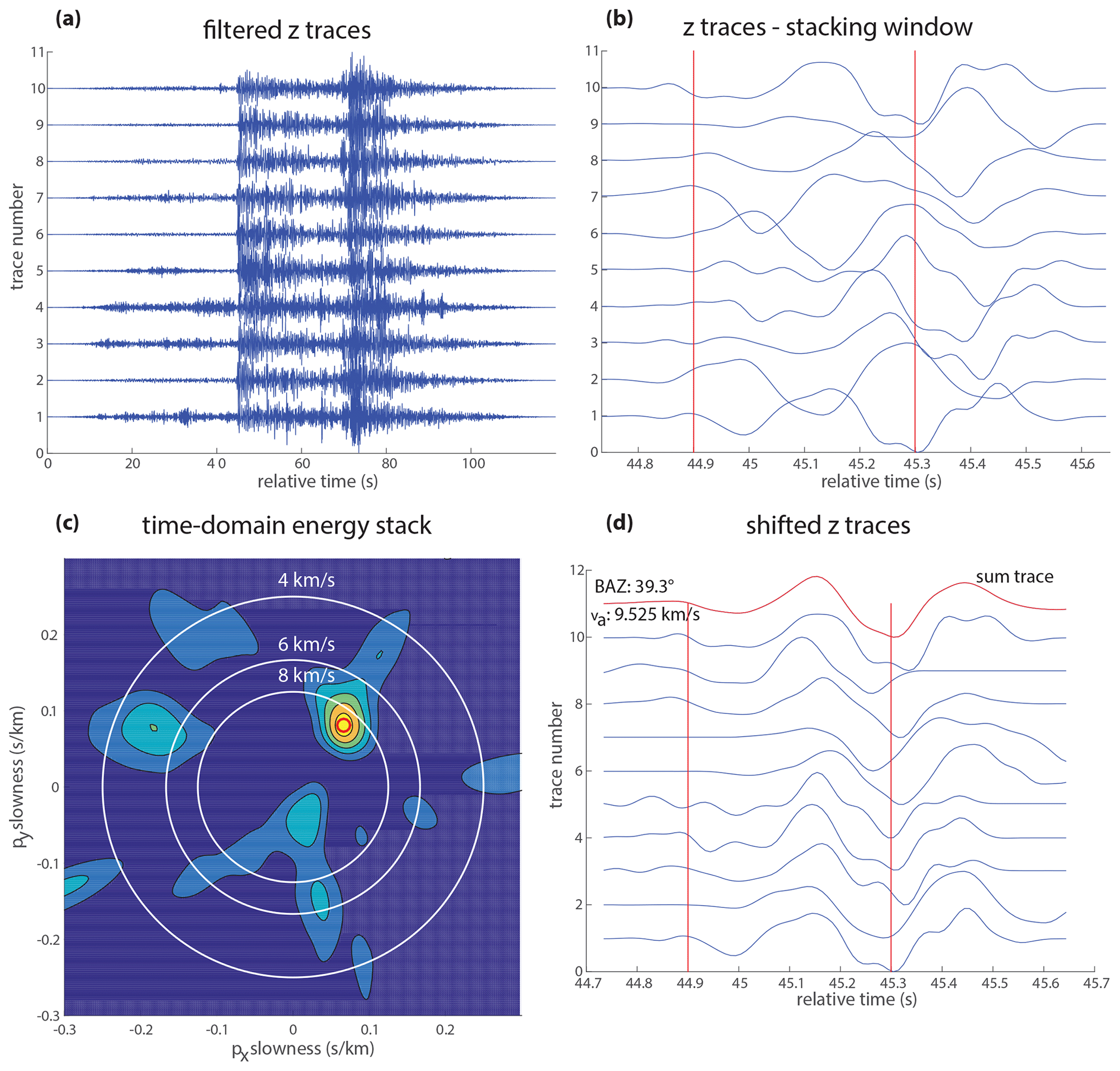
Figure 8Array analysis of an event of 14 February 2015 at 07:08:55 UTC that occurred close to the CIR, east of Rodrigues Island, which is listed in the USGS catalogue. (a) Vertical-component traces. (b) Zoom-in of the P waveforms. (c) Beam energy as a function of horizontal slowness components sx and sy. (d) Shifted traces and beam (red trace) corresponding to the maximum indicated in (c). The back azimuth of this event is determined at about 39∘ with an apparent velocity of 9.5 km s−1.
The larger earthquakes along the CIR picked up by the global networks are listed in the earthquake database provided by USGS (https://earthquake.usgs.gov/earthquakes/search/, last access: August 2016). Thirty events reported in the catalogue were also recorded by Rodrigues array. Six of these events exhibit sufficient signal-to-noise ratio to perform the array analysis for a comparison with the USGS-reported locations.
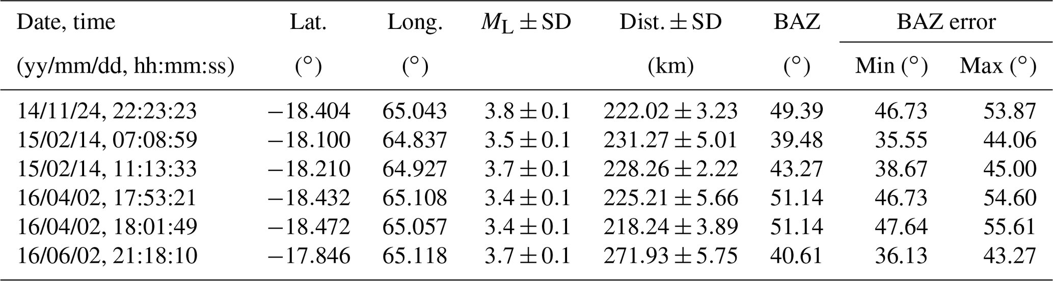
Geographical coordinates, origin times, and magnitudes for the six events obtained from the array analysis are shown in Table 1. They can be compared with the results provided by the USGS catalogue (Table 2). Magnitudes obtained from the array analysis are slightly lower than those reported by USGS. This may be in part due to different magnitude scales used (local magnitude versus body wave magnitude). Ristau (2009) compared different magnitude scales for New Zealand earthquakes, where mb was lower than ML for deep focus (>33 km) events but the results were fairly consistent for shallow (≤33 km) earthquakes. In the current study, we consider that the data are not sufficient to derive a relationship between mb and ML. Amplitude variations related to the different radiation directions relevant for regional (at Rodrigues Island) and teleseismic recordings may also play a role. In addition, the amplitudes for the dominantly horizontal Pn ray paths from the recordings at Rodrigues may be more affected by regional attenuation processes, as described further in the next section.
Table 1Events from USGS catalogue located using the Rodrigues array.

The array analysis for the six events was performed as described above. An example is given in Figs. 7 and 8 for an event of 14 February 2015 at 07:08:59 UTC. P and S phases are clearly visible and the dominant frequency of the P wave arrival for this event is about 3.5 Hz. From the array analysis, we obtain a clear maximum for , which corresponds to a back azimuth and apparent velocity . The time shifts derived from the obtained slowness value according to (where δrj corresponds the position of station j with respect to the reference station) yield a good alignment of the P wave signal.
The mean distance of the event was calculated using distances from all the stations that provided clear P and S phases. Figure 7 shows the three-component seismogram and the STA ∕ LTA trigger function to identify the onset times. The arrival-time difference of 24.63 s corresponds to a distance of 231 km (based on the model described above). For the magnitude, we derive ML=3.5.
For three events, we obtain small variations in back azimuth, which are well within the error estimations. Events on 24 November 2014 at 22:23:23 UTC, 2 April 2016 at 18:01:49 UTC, and 2 June 2016 at 21:18:10 UTC show differences of about 11, 9, and 7∘, respectively. Array-derived distances from the reference station are generally smaller than those given in USGS catalogue, except for the event of 2 April 2016 at 17:53:21 UTC, where the distance obtained from array analysis is well within the error range.
We attribute these differences to local inhomogeneities not accounted for in the array analysis and to the simple 1-D model used for the distance estimates (in addition to possible errors in the global locations). Figure S3 in the Supplement shows a comparison of the results obtained by the array analysis with those provided by the USGS catalogue. Generally, the results agree well. On average, location differences are about 17 km, which is a reasonable value considering the uncertainties of the approach.
Using the array technique, we were able to detect and locate 63 earthquakes in the Rodrigues–CIR region that are not reported by the USGS catalogue (Fig. 9). The details of all the events, such as event location, origin time, and magnitude are summarized in Table S1 (Supplement). The magnitudes of these events range from 1.6 to 3.7 and are spread out in a region of radius up to 600 km from the array. The nearest event to Rodrigues Island (ML 1.6) occurred on 12 February 2016 at 19:21:45 UTC to the north of the island at a distance of about 36 km.
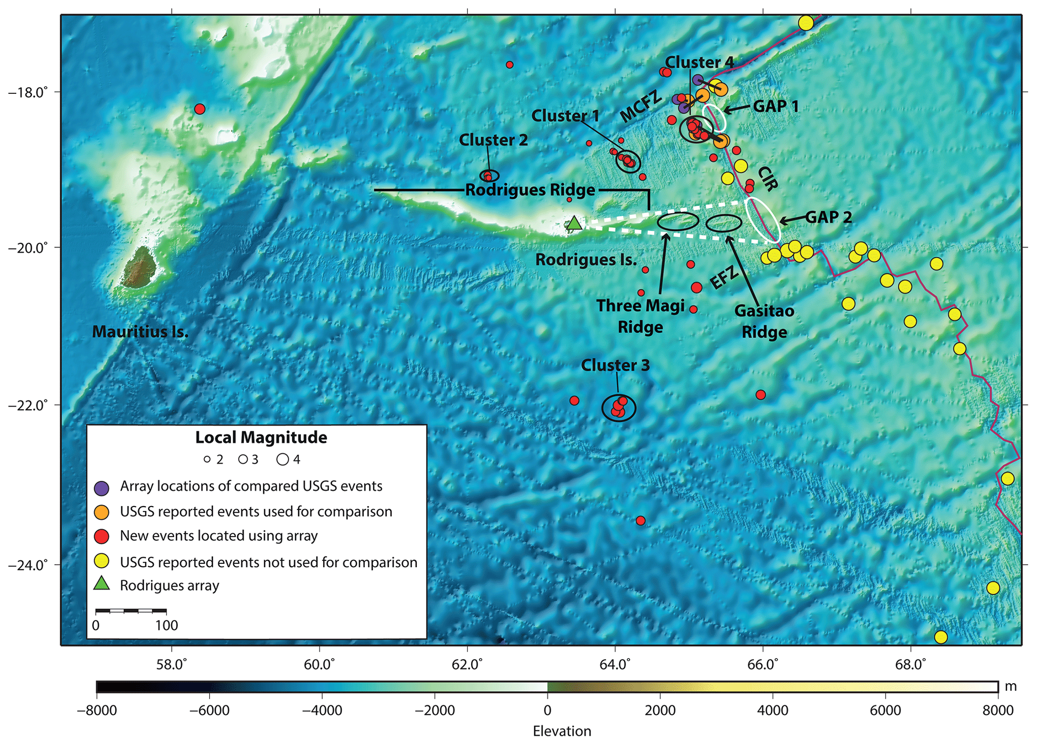
Figure 9Locations of new events (and clusters) detected and located using array methods are shown by red circles. The purple circles represent event locations from the array analysis in comparison to the events (orange circles) from the USGS catalogue between September 2014 and June 2016. The black bars pair the respective events. Yellow circles denote events from the USGS catalogue for the same recording period that were not (clearly) detected at the Rodrigues array and that were therefore not used for a comparison. The empty GAP 1 and GAP 2 have been demarcated by white ellipses. The dashed white line marks the possible region of partially molten material below the eastern extension of Rodrigues Ridge. CIR, Central Indian Ridge (solid red line); MCFZ, Marie-Celeste fracture zone; and EFZ, Egeria fracture zone.
Of the 63 events, 51 are located off the ridge axis and can therefore be classified as intraplate earthquakes. A total of 12 events were located very close to the ridge axis. A total of 24 events occur between back azimuths of 29∘ and 42∘ at a distance of about 120 km and exhibit magnitudes between 1.6 and 3.0 (Fig. 9). Almost all events in this back azimuth (20) occur from March to April 2015 (Fig. 10). Magnitudes for this cluster of earthquakes are variable and do not follow a certain (main shock–aftershock) pattern (Cluster 1, Table S2 in the Supplement). Detailed bathymetry indicates a step-like non-transform discontinuity at the southeastern end of this chain of events.
Three more clusters occur to the east, south, and northwest of Rodrigues Island at distances of about 265, 140, and 220 km with 6, 3, and 7 events, respectively. This is further corroborated by Fig. 10, where events' longitude and latitude are plotted as functions of time. Also shown is the monthly number of events, which exhibits a clear maximum for March 2015 in relation to the activity of Cluster 1. As Cluster 4 (∼220 km east of Rodrigues Island) is close to the ridge axis, events of this cluster are not considered as intraplate events.
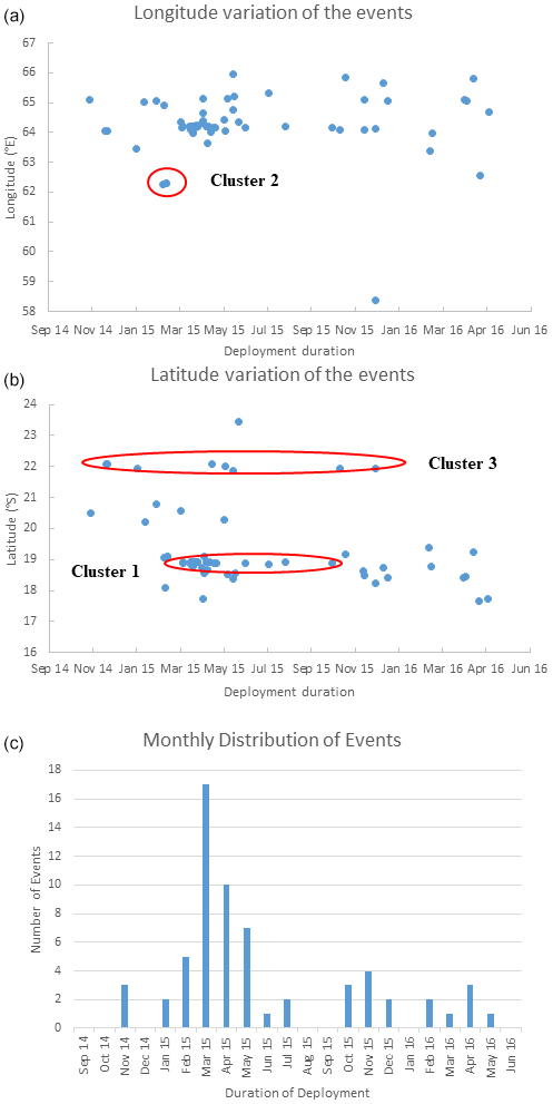
Figure 10Variation in longitude (a) and latitude (b) of the events detected and located using Rodrigues array. Monthly distribution of the events is shown in (c). The solid red line in (b) marks the events for Cluster 1 (∼120 km northeast of Rodrigues Island), Cluster 2 (∼140 km northwest of Rodrigues Island), and Cluster 3 (∼265 km south of Rodrigues Island).
As shown in the sensitivity test provided in the supplementary information (Figs. S1 and S2), the location errors for Cluster 1 are much smaller as compared to Cluster 3, partially owing to their distance from the Rodrigues array. Some influence of anisotropic velocity variation may also be possible, as studies by Barruol and Fontaine (2013) and Scholz et al. (2018) suggest fast-axis directions trending east–west around the Rodrigues–CIR region.
Various mechanisms providing explanation to the cause of intraplate seismicity have been proposed previously. De Long et al. (1977) suggested that different lithospheric ages across the fracture zones, as also observed in the Rodrigues–CIR region, are related to differential subsidence causing stresses and hence earthquakes. Similarly, Collette (1974) and Turcotte (1974) suggested thermal contraction due to different ages of the oceanic crust (Müller et al., 2008) as another possible mechanism. This may be substantiated by the seismicity observed in clusters 2 and 3 as they occur along possible prolongations of fracture zones. Mantle-derived carbon dioxide discharge (e.g., Bräuer et al., 2003; Gold and Soter, 1984; Irwin and Barnes, 1980) can also provide an explanation for the intraplate seismic activity around the Rodrigues–CIR region, as most of the detected events occur in clusters 1 and 4, which are not related to fracture zones. In continental regions, similar clustering has been associated with carbon dioxide discharge (e.g., Lindenfeld et al., 2012).
It is interesting to note that the two seismic gaps along the slow-spreading CIR, as indicated above, still show no seismic activity based on the new data. Thus, these seismic gaps may indeed represent an anomalous section of the CIR that is deforming aseismically. The anomalous nature of this region is further corroborated by the fact that globally recorded events from the farther southern section of CIR are not detected by the array (see events south of in Fig. S3 in the Supplement). This could be explained by a more extended region of partially molten material in the upper mantle that causes significant attenuation of wave amplitudes for the corresponding ray paths (Fig. 9), as also suggested by Mazzullo et al. (2017). In combination with the absence of any seismic activity along Rodrigues Ridge, this may be taken as evidence for the explanation of Rodrigues Ridge as a surface expression of the interaction of the Réunion Hotspot with the CIR through a sublithospheric flow channel (Morgan, 1978; Dyment et al., 2007; Bredow et al., 2017). Another explanation for the lack of seismicity in GAP 1 and GAP 2 could be excessive magmatism and a resulting relatively thin lithosphere that does not support large earthquakes, as suggested by Cannat (1996) and Grevemeyer et al. (2013).
Based on hydro-acoustic data, similar seismic gaps were also observed along the intermediate-spreading Southeast Indian Ridge (Tsang-Hin-Sun et al., 2016) and the slow-spreading Mid-Atlantic Ridge (Escartin et al., 2008; Simao et al., 2010), where events were focused on ridge segment ends. This uneven distribution of seismicity along CIR, thus suggests segment-scale variation in lithosphere structure, as also observed in Southeast Indian Ridge (Tsang-Hin-Sun et al., 2016) and Mid-Atlantic Ridge (Goslin et al., 2012).
We installed a 10-station seismological array on Rodrigues Island to study the seismicity along a remote section of the CIR and nearby areas including Rodrigues Ridge. The results show that array analysis provides a valuable tool to study earthquake activity in oceanic regions which are relatively inaccessible otherwise. The region around Rodrigues Island clearly shows evidence of intraplate seismicity. Of the 63 events detected by Rodrigues array, the majority are located within Cluster 1 at a distance of ∼120 km from the island with back azimuths between 29 and 42∘. The local magnitude (ML) of the events detected ranges between 1.6 and 3.7. Three additional event clusters were identified. Possible explanations for the off-axis seismic activities are CO2 degassing from the mantle and differential thermal contraction, whereas events in Cluster 4, being close to ridge axis, are not considered as intraplate events. The lack of seismic activity along both Rodrigues Ridge and a section of the CIR to the east of Rodrigues Island (GAP 2) may be explained by partially molten upper-mantle material, possibly in relation to the proposed material flow from the Réunion plume and the CIR (Morgan, 1978; Dyment et al., 2007; Bredow et al., 2017). This explanation is further supported by the observation that relatively strong seismic events from the CIR, east to southeast of Rodrigues Island (which are listed in the USGS catalogue) are not detected by the array. However, a detailed geodynamic model for the ridge–plume interaction in this region is still needed. We anticipate that longer-term deployments of seismic arrays on Rodrigues and other remote islands of Mauritius, such as Agalega and St. Brandon, will provide further constraints on the seismic gaps along the CIR and the intraplate seismicity of the region. Dedicated deployment of Ocean Bottom Seismometers or Hydrophones (OBS/H) at or near these targets is another option for future studies.
The data used in this research are currently restricted. The data will be publicly available from GEOFON data archive of Deutsches Geoforschungszentrum Potsdam as from July 2021.
The supplement related to this article is available online at: https://doi.org/10.5194/se-11-2557-2020-supplement.
MS and GR participated in field work and data analyses, provided their interpretations, and wrote the article.
The authors declare that they have no conflict of interest.
The study presented here was funded by the Mauritius Oceanography Institute, Mauritius, through the Ministry of Finance and by the Deutsche Forschungsgemeinschaft (DFG) through a grant to GR.
The instruments for the temporary array were provided by the Geophysical Instrument Pool Potsdam at the Deutsches Geoforschungszentrum, Potsdam. We wish to thank the Government of Mauritius for allowing us to carry out the study, as well as the MOI and Rodrigues Regional Assembly (RRA) for the support provided during the fieldwork. We thank Jérôme Dyment of IPGP for his suggestions and comments regarding the bathymetry around the CIR region. We also thank Frederik Link, Corrado Surmanowicz, Olivier Pasnin, and Shane Sunassee for providing help during field work at Rodrigues Island. We thank the reviewers for the thorough reviews that helped to improve the paper.
This research has been supported by the German Research Foundation (grant no. RU 886/7-1).
This open-access publication was funded
by the Goethe University Frankfurt.
This paper was edited by Irene Bianchi and reviewed by two anonymous referees.
Barruol, G. and Fontaine, F. R.: Mantle flow beneath La Réunion hotspot track from SKS splitting, Earth Planet. Sci. Lett., 362, 108–121, https://doi.org/10.1016/j.epsl.2012.11.017, 2013.
Becker, T. W., and Faccenna, C.: Mantle conveyor beneath the Tethyan collisional belt, Earth Planet. Sci. Lett., 310, 453–461, https://doi.org/10.1016/j.epsl.2011.08.021, 2011.
Bergman, E. A. and Solomon, S. C.: Oceanic intraplate earthquakes: Implications for local and regional intraplate stress, J. Geophy. Res. Solid Earth, 85, 5389–5410, 1980.
Bergman, E. A., Nábělek, J. L., and Solomon, S. C.: An extensive region of off-ridge normal-faulting earthquakes in the southern Indian Ocean, J. Geophy. Res.-Sol. Ea., 89, 2425–2443, 1984.
Bräuer, K., Kampf, H., Sträuch, G., and Weise, S. M.: Isotopic evidence (3He∕4He, 13CCO2) of fluid triggered intraplate seismicity, J. Geophys. Res., 108, 2070, https://doi.org/10.1029/2002JB002077, 2003.
Bredow, E., Steinberger, B., Gassmöller, R., and Dannberg, J.: How plume-ridge interaction shapes the crustal thickness pattern of the R éunion hotspot track, Geochem. Geophy. Geosy., 18, 2930–2948, https://doi.org/10.1002/2017GC006875, 2017.
Cannat, M.: How thick is the magmatic crust at slow spreading oceanic ridges?, J. Geophys. Res.-Sol. Ea., 101, 2847–2857, https://doi.org/10.1029/95JB03116, 1996.
Christensen, N. I.: Serpentinites, peridotites, and seismology, Int. Geol. Rev., 46, 795–816, https://doi.org/10.2747/0020-6814.46.9.795, 2004.
Collette, B. J.: Thermal contraction joints in a spreading seafloor as origin of fracture zones, Nature, 251, 299–300, 1974.
Conrad, C. P. and Behn, M. D.: Constraints on lithosphere net rotation and asthenospheric viscosity from global mantle flow models and seismic anisotropy, Geochem. Geophy. Geosy., 11, Q05W05, https://doi.org/10.1029/2009GC002970, 2010.
De Long, S. E., Dewey, J. F., and Fox, P. J.: Displacement history of oceanic fracture zones, Geology, 5, 199–202, 1977.
Duncan, R. A. and Hargraves, R. B.: 40Ar∕39Ar Geochronology of basement rocks from the Mascarene plateau, the Chagos bank and the Maldives ridge, in: Proceedings of Ocean Drilling Program, Scientific Results, Vol. 115, College Station, TX: Ocean Drilling Program, 43–51, 1990.
Dyment, J., Hémond, C., Guillou, H., Maia, M., Briais, A., and Gente, P.: Central Indian Ridge and Reunion hotspot in Rodrigues area: Another type of ridge-hotspot interaction?, Eos Trans. AGU, 82(47), Fall Meet. Suppl., Abstract T31D–05, 2001.
Dyment, J., Lin, J., and Baker, E. T.: Ridge-hotspot interactions: What mid-ocean ridges tell us about deep earth processes, Oceanography, 20, 102–115, 2007.
Escartín, J., Smith, D. K., Cann, J., Schouten, H., Langmuir, C. H., and Escrig, S.: Central role of detachment faults in accretion of slow-spreading oceanic lithosphere, Nature, 455, 790–794, 2008.
Fontaine, F. R., Barruol, G., Tkalčić, H., Wölbern, I., Rümpker, G., Bodin, T., and Haugmard, M.: Crustal and uppermost mantle structure variation beneath la Réunion hotspot track, Geophys. J. Int., 203, 107–126, 2015.
Grevemeyer, I., Reston, T. J., and Moeller, S.: Microseismicity of the Mid-Atlantic Ridge at 7∘ S–8∘15′ S and at the Logatchev Massif oceanic core complex at 14∘40′ N–14∘50′ N, Geochem. Geophy. Geosy., 14, 3532–3554, 2013.
Gutenberg, B. and Richter, C. F.: Seismicity of the Earth, Geol. Soc. Am. Spec. Pap., 34, 1–126, 1941.
Gold, T. and Soter, S.: Fluid ascent through the solid lithosphere and its relation to Earthquakes, Pure Appl. Geophys., 122, 492–530, 1984.
Goslin, J., Perrot, J., Royer, J. Y., Martin, C., Lourenço, N., Luis, J., Dziak, R. P., Matsumoto, H., Haxel, J., Fowler, M. J., and Fox, C. G.: Spatiotemporal distribution of the seismicity along the Mid-Atlantic Ridge north of the Azores from hydroacoustic data: Insights into seismogenic processes in a ridge–hot spot context, Geochem. Geophy. Geosy., 13, https://doi.org/10.1029/2011GC003828, 2012.
Harjes, H. and Henger, M.: Array-Seismologie, Z. Geophys., 39, 865–905, 1973.
Haubrich, R. A.: Array design, B. Seismol. Soc. Am., 58, 977–991, 1968.
Havskov, J. and Ottemoller, L.: SeisAn Earthquake analysis software, Seismol. Res. Lett., 70, 532–534, https://doi.org/10.1785/gssrl.70.5.532, 1999.
Husebye, E. and Ruud, B.: Array seismology – past, present and future developments, Observ. Seismol., 23–153, 1989.
Irwin, W. P. and Barnes, I.: Tectonic relations of carbon dioxide discharges and earthquakes, J. Geophys. Res., 85, 3115–3121, 1980.
Kong, L. S., Solomon, S. C., and Purdy, G. M.: Microearthquake characteristics of a mid-ocean ridge along-axis high, J. Geophys. Res.-Sol. Ea., 97, 1659–1685, https://doi.org/10.1029/91JB02566, 1992.
Krishna, M. R., Verma, R., and Arora, S.: Near-ridge intraplate earthquakes in the Indian Ocean, Mar. Geol., 147, 109–122, 1998.
Leva, C., Rümpker, G., Link, F., and Wölbern, I.: Mantle earthquakes beneath Fogo volcano, Cape Verde: Evidence for subcrustal fracturing induced by magmatic injection, J. Volcanol. Geotherm. Res., 386, 106672, https://doi.org/10.1016/j.jvolgeores.2019.106672, 2019.
Lindenfeld, M., Rümpker, G., Link, K., Koehn, D., and Batte, A.: Fluid-triggered earthquake swarms in the Rwenzori region, East African Rift – Evidence for rift initiation, Tectonophysics, 566, 95–104, https://doi.org/10.1016/j.tecto.2012.07.010, 2012.
Mazzullo, A., Stutzmann, E., Montagner, J. P., Kiselev, S., Maurya, S., Barruol, G., and Sigloch, K.: Anisotropic tomography around La Réunion island from Rayleigh waves, J. Geophys. Res.-Sol. Ea., 122, 9132–9148, https://doi.org/10.1002/2017JB014354, 2017.
Morgan, W. J.: Rodriguez, Darwin, Amsterdam, ..., a second type of hotspot island, J. Geophys. Res.-Sol. Ea., 83, 5355–5360, 1978.
Müller, R. D., Sdrolias, M., Gaina, C., and Roest, W. R.: Age, spreading rates, and spreading asymmetry of the world's ocean crust, Geochem. Geophy. Geosy., 9, https://doi.org/10.1029/2007GC001743, 2008.
Okal, E. A.: Oceanic intraplate seismicity, Annu. Rev. Earth Plan. Sci., 11, 195–214, 1983.
Ristau, J.: Comparison of magnitude estimates for New Zealand earthquakes: Moment magnitude, local magnitude, and teleseismic body-wave magnitude, B. Seismol. Soc. Am., 99, 1841–1852, https://doi.org/10.1785/0120080237, 2009.
Rost, S. and Thomas, C.: Array Seismology: Methods and applications, Rev. Geophys., 40, https://doi.org/10.1029/2000RG000100, 2002.
Saddul, P., Nelson, B. W., and Jahangeer-Chojoo, A.: Mauritius: A Geomorphological Analysis, vol. 3, Mahatma Gandhi Institute, Mauritius, 2002.
Scholz, J. R., Barruol, G., Fontaine, F. R., Mazzullo, A., Montagner, J. P., Stutzmann, E., Michon, L., and Sigloch, K.: SKS splitting in the Western Indian Ocean from land and seafloor seismometers: Plume, plate and ridge signatures, Earth Planet. Sci. Lett., 498, 169–184, https://doi.org/10.1016/j.epsl.2018.06.033, 2018.
Schweitzer, J., Fyen, J., Mykkeltveit, S., and Kværna, T.: Manual of seismological observatory practice, 2002.
Simao, N., Escartin, J., Goslin, J., Haxel, J., Cannat, M., and Dziak, R.: Regional seismicity of the Mid-Atlantic Ridge: observations from autonomous hydrophone arrays, Geophys. J. Int., 183, 1559–1578, 2010.
Sykes, L. R. and Sbar, M. L.: Intraplate earthquakes, lithospheric stresses and the driving mechanism of plate tectonics, Nature, 245, 298–302, 1973.
Tsang-Hin-Sun, E., Royer, J. Y., and Perrot, J.: Seismicity and active accretion processes at the ultraslow-spreading Southwest and intermediate-spreading Southeast Indian ridges from hydroacoustic data, Geophys. J. Internat., 206, 1232–1245, 2016.
Turcotte, D. L.: Are transform faults thermal contraction cracks?, J. Geophys. Res., 79, 2573–2577, 1974.
Wolfe, C. J., Purdy, G. M., Toomey, D. R., and Solomon, S. C.: Microearthquake characteristics and crustal velocity structure at 29∘ N on the Mid-Atlantic Ridge: The architecture of a slow spreading segment, J. Geophys. Res.-Sol. Ea., 100(B12), 24449–24472, https://doi.org/10.1029/95JB02399, 1995.