Towards plausible lithological classification from geophysical inversion: honouring geological principles in subsurface imaging

We propose a methodology for the recovery of lithologies from geological and geophysical modelling results and apply it to field data. Our technique relies on classification using self-organizing maps (SOMs) paired with geoscientific consistency checks and uncertainty analysis. In the procedure we develop, the SOM is trained using prior geological information in the form of geological uncertainty, the expected spatial distribution of petrophysical properties and constrained geophysical inversion results. We ensure local geological plausibility in the lithological model recovered from classification by enforcing basic topological rules through a process called “post-regularization”. This prevents the three-dimensional recovered lithological model from violating elementary geological principles while maintaining geophysical consistency. Interpretation of the resulting lithologies is complemented by the estimation of the uncertainty associated with the different nodes of the trained SOM. The application case we investigate uses data and models from the Yerrida Basin (Western Australia). Our results generally corroborate previous models of the region but they also suggest that the structural setting in some areas needs to be updated. In particular, our results suggest the thinning of one of the greenstone belts in the area may be related to a deep structure not sampled by surface geological measurements and which was absent in previous geological models.

1 Introduction

The idea of geoscientific integration is not new and has been advocated since the inception of quantitative geoscientific studies involving geophysics and during the advances of geophysics as a discipline (see, for instance, Wegener, 1920; Nettleton, 1949; Towles, 1952; Jupp and Vozoff, 1975; Lines et al., 1988; Li and Oldenburg, 2000). In the natural resource sector, the exploitation of the fundamental complementarity between geology and geophysics in modelling the same object (the Earth) has been recognized as one of the pre-requisites to exploration success as early as the 1940s during the early years of the Society of Exploration Geophysicists (Eckhardt, 1940; Green, 1948). Numerous authors have since tackled the issue of integrating petrophysical and geological information to model geophysical quantities (seismic velocities, mass density, etc.) through inversion, with an increasing trend in the past 15 years or so (see, for instance, references reviewed in Lelièvre and Farquharson 2016; Meju and Gallardo 2016; Moorkamp et al., 2016; Giraud et al., 2017). In contrast, the recovery of geological quantities from geophysical inversion has seen much less effort. Recent studies have started to rectify this by proposing the idea of lithological differentiation of inversion results (Paasche et al., 2010; Sun and Li, 2015; Paasche and Tronicke, 2007), which consists of the identification of lithologies from inversion results. While lithological differentiation is expected to hold much potential in mineral exploration, it still remains underexplored (Li et al., 2019).

In oil and gas exploration scenarios, seismic facies analyses and classification using techniques developed for what is commonly called machine learning (neural networks, support vector machine algorithms, etc.) have become popular in recent years (Zhao et al., 2015; Chopra and Marfurt, 2018; Wrona et al., 2018; Zhang et al., 2018). This was driven by the need for quantitative interpretation methods in the geosciences and by the “renaissance” phase machine learning went through after 2006 (Goodfellow et al., 2016, chap. 5). Once recovered, spatial facies distribution can be used for geological interpretation and downstream decision making. However, like all modelling results, the identification of facies or lithologies using machine learning relies upon statistical models and is affected by ambiguity and uncertainty. One reason for this is that validation datasets are usually treated as the ground “truth”, while they are fraught with uncertainty. For instance, the interpretation of borehole data or outcrops with their uncertainty can lead to significantly different models honouring geological measurements equally well (Wellmann et al., 2010; de la Varga et al., 2019; Pakyuz-Charrier et al., 2018a, b, c).

Lithologies (or facies) can be characterized by a broad range of rock properties that are the result of geological processes, such as weathering, compaction, metamorphism and deformation. These physical processes are usually non-linear, especially when in combination, and produce complex representations of different lithotypes which are difficult to discriminate from geophysical data. In this context, one possible solution is to use neural networks for lithological classification, as they are “universal approximators” (van der Baan and Jutten, 2000). As a consequence, however, lithological classification is affected by uncertainty from the data used to train and validate the algorithm. Such uncertainty is difficult to quantify and is rarely estimated or even considered.

To date, whether it be in oil and gas or mining exploration, uncertainty in recovered lithologies is a research avenue, which, to the best of our knowledge, only a few authors have addressed. Sun and Li (2019) assess uncertainty by varying the number of clusters in their lithological differentiation scheme, and Bauer et al. (2003) classify lithologies and estimate the resolution of their results using synthetic data. As a result of the lack of comprehensive uncertainty analyses, practitioners often lack quantitative, robust uncertainty modelling necessary to inform interpretation or risk evaluation (Jessell et al., 2018). In addition, apart from Zhao et al. (2017), who account for seismic data-driven stratigraphy in their seismic facies classification, established workflows relying on neural networks to identify facies or lithologies in three dimensions give little to no consideration of geological information and rules for their classification.

To complement existing methodologies, we propose a solution that partially addresses the lack of consideration given to geological information during classification. We introduce a general post-processing (i.e. post-inversion) workflow for the recovery of lithologies from geoscientific modelling results and the estimation of the related uncertainty. For this purpose, we complement existing classification techniques by ensuring the geological and geophysical consistency of, and estimating the confidence in, the recovered lithologies. Using an artificial neural network trained in a fully controlled environment (all variables in the model used for training being perfectly known) with attributes characterizing the inversion results, we perform lithological classification applying plausibility filters relying on geological principles, which we refer to as “geological post-regularization”. The application of geological post-regularization is to reduce the non-geological character of models obtained through classification. After classification, we calculate the frequentist probability of the different lithologies (i.e. apparition frequency relative to all lithologies) associated with each unit of the self-organizing map (SOM) and report it in each model cell discretizing the studied area for interpretation.

The methodology we propose can serve two main objectives. Our first objective is to introduce a methodology that is made efficient by leveraging existing geoscientific inputs and prior information, and cost-effective by imposing requirements that do not exceed the computational power available on a personal computer. Secondly, our aim is to complement inversion workflows by providing a general, automated method to derive a non-deterministic lithological interpretation of inversion results. Thirdly, we propose a real-world application based on a case study in the Yerrida Basin (Western Australia), where we build upon recent work by Giraud et al. (2019a) and Lindsay et al. (2018), who performed the geophysical inversion and geological modelling of data collected in the area, respectively.

In this work, lithologies are identified though a classification technique relying on a simple artificial neural network. We chose SOMs (Kohonen, 1982a, b), a well-established algorithm that has been successfully applied to seismic facies classification and geological mapping purposes (Chang et al., 2002; Klose, 2006; Köhler et al., 2010; Bauer et al., 2012; Carneiro et al., 2012; Du et al., 2015; Roden et al., 2015). We first train and test the SOMs using data extracted from a semi-synthetic dataset (i.e. a geophysical inversion feasibility study based on geological and petrophysical field data) assumed to represent the geophysical characteristics of the studied area. We utilize this controlled environment to estimate the accuracy our predictions for each class identified in the studied volume without the errors associated with well positioning or lithology interpretation errors. We then use the trained network to perform classification using field data only. We obtain, for each model cell, a suite of frequentist probabilities for each lithology observed in the area. In both cases, geological post-regularization is applied before the calculation of uncertainty metrics to ensure the geological consistency of the results.

The rest of this paper develops as follows. Section 2 provides the theoretical background necessary to reproduce the work presented. It first briefly describes the geophysical and geological modelling schemes (Sect. 2.1) used to obtain the models that are used as input for classification using SOM (Sect. 2.2). Post-regularization as applied to such classified lithologies (Sect. 2.3) and the related uncertainty analysis in terms of prediction accuracy and geophysical consistency is then detailed (Sect. 2.4). Following this, Sect. 3 presents an application case using data from the Yerrida Basin (Western Australia), which was investigated using gravity data, petrophysical and geological information. Geological and geophysical modelling results are first summarized and the rules defining the post-regularization operator in the area are introduced (Sect. 3.1). The classification of results from geological and geological modelling and post-regularization is then presented alongside the related uncertainty analysis, supporting a potential re-interpretation of the geological model of the area (Sect. 3.2). The discussion and conclusion sections follow and complete this contribution.

2 Methodology for geoscientific modelling and classification

In this section, we first introduce essential information about the geophysical and geological modelling used as a pre-requisite to this study. We then introduce the utilization of SOM and the tools we developed in sufficient detail to allow the reproducibility of the procedure.

2.1 Geophysical and geological modelling

Inverse geophysical modelling was performed using the least-square inversion TOMOFAST-X platform. This inversion platform enables the use of a series of constraints as detailed in Martin et al. (2018), Giraud et al. (2019a, b). Constraints are enforced through a minimum-structure gradient regularization approach where weights vary locally accordingly with geological uncertainty (Giraud et al., 2019a). The cost function to minimize is given as

$$\begin{array}{}\text{(1)}& \begin{array}{rl}\mathit{\theta }\left(d,m\right)& ={∥{\mathbf{W}}_{\mathrm{d}}\left(d-g\left(m\right)\right)∥}_{\mathrm{2}}^{\mathrm{2}}+{\mathit{\alpha }}_{\mathrm{m}}{∥{\mathbf{W}}_{\mathrm{m}}\left(m-m_{\mathrm{p}}\right)∥}_{\mathrm{2}}^{\mathrm{2}}\\ & +{\mathit{\alpha }}_{\mathrm{s}}{∥{\mathbf{W}}_{\mathrm{s}}\mathrm{\nabla }m∥}_{\mathrm{2}}^{\mathrm{2}},\end{array}\end{array}$$

where d represents observed data and m is the model; g is the forward operator calculating the predicted data m produces; m_p is the prior model. In Eq. (1), subscripts d, m and s refer to data, model and smoothness, respectively. In this contribution, W_d is a diagonal matrix where each element is equal to the inverse of the sum of squares of the geophysical measurements; W_m and W_s are diagonal covariance matrices; here, W_m is the identity matrix. The scalars α_m and α_s are weights controlling the relative importance of the different terms in the equation; ∇ is the spatial gradient operator. The last term of the Eq. (1), the smoothness term, constrains the structural features of the inverted model. The values in diagonal matrix W_s are determined from prior information. In the presented work, W_s is obtained from geological modelling results and is a proxy for geological uncertainty

The matrix W_s is calculated following Giraud et al. (2019a), who use the probabilistic geological modelling approach described in Pakyuz-Charrier et al. (2018b, c, 2019). In the case of gravity inversion as presented here, the complete Bouguer anomaly of density contrast model m is calculated as the product of the Jacobian matrix G with model m. Therefore, we have g(m)=Gm.

Geological uncertainty is estimated from probabilistic geological modelling. During this process, an ensemble of geological models is generated using the Monte Carlo uncertainty estimator (MCUE) of Pakyuz-Charrier et al. (2018a, b, c, 2019). MCUE relies on the perturbation of orientation measurements (interfaces and foliations) defining structures of a reference geological model accordingly with their uncertainty. From this series of models, geological uncertainty can be estimated (Wellmann and Regenauer-Lieb, 2012) through calculation of Shannon's entropy (Shannon, 1948) for the simulated geological models. Shannon's entropy, which can be used as a proxy for geological uncertainty, indicates how well geological information constrains the model locally. It can be used to constrain inversion in a structural sense when integrated in W_s as per Eq. (1) (Giraud et al., 2019a).

More detailed information about the usage of MCUE results in geophysical inversion can be found in Giraud et al. (2017, 2018a, 2019a, b).

2.2 Classification using SOM

The SOM artificial neural network relies on competitive, non-supervised learning. The relative simplicity and the efficiency of the SOM algorithm has made it a popular tool for classification, data imputation, visualization and dimensionality reduction (Vesanto and Alhoniemi, 2000; Kalteh et al., 2008; Miljkovic, 2017; Klose, 2006; Kohonen, 1998, 2013; Roden et al., 2015; Martin and Obermayer, 2009). In essence, it consists in the projection of the SOM's latent space onto a manifold of superior dimension (i.e. our dataset). This map, which can be 2-D or 3-D, is made of a predefined number of interconnected neurons (also referred to as “nodes” or “units”) that have a fixed network configuration. Projection occurs during the training phase, where the locations of the neurons in the manifold are iteratively adjusted so approximation is optimal.

In this study, we follow common practice by training two-dimensional (2-D) maps using a hexagonal lattice topology and applying a Gaussian-shaped neighbourhood function. We chose to use a 2-D map for the sake of simplicity after our testing revealed that other configurations did not improve results significantly. The hexagonal lattice topology seemed to provide better results than square lattice topology using the dataset we present here.

Ideally, the SOM should be trained in a controlled environment where all the variables used are perfectly known, which motivates the utilization of synthetic geophysical data. We calculate such data from a geological structural framework derived from real-world field geological and petrophysical field measurement data in the same fashion as for a geophysical feasibility study. The training and tests datasets are comprised of the following variables:

1. starting model for inversion m_start;

2. inverted model m_inv;

3. geological uncertainty W_s;

4. spatial gradient in the inverted model ${∥\mathrm{\nabla }{m}_{\mathrm{inv}}∥}_{\mathrm{2}}$; and

5. most likely lithology obtained from geological modelling (training lithological model).

The starting model is obtained from prior information. Here, it is the expected petrophysical property model from geological modelling. Each datum from the training and tests datasets is a vector $x\mathit{ϵ}{R}^{n_{\mathrm{v}}}$, with a number of variables n_v=5, where x(5) is the lithology assigned to this unit. This choice of training variables was motivated by the necessity to account for the available information in terms of geological modelling and measurements, uncertainty and structural setting. The starting model for inversion encapsulates the pre-inversion state of knowledge. The inverted model comprises the update of this model using information extracted from geophysical measurements and translated into a 3-D model. The lithological model refers directly to the interpreted geological observations of the area. The spatial gradients of the inverted models provide structural information about the location of the geological units that can be recovered by interpretation from the inverted density contrast model.

During training, we examine SOM quality using quantization error Q and lithology prediction accuracy. Quantization error “measures the average distance between each data vector and its best matching unit [BMU]” (Uriarte and Martín, 2005), thereby indicating how well the different BMUs approximate the dataset. It can be interpreted as analogous to a misfit between calculated and observed data. The mean quantization error Q of the SOM is expressed as follows for n data vectors x_i:

$$\begin{array}{}\text{(2)}& Q\left(x,\mathrm{BMU}\right)={\displaystyle \frac{\mathrm{1}}{n}}{\sum }_{i=\mathrm{1}}^n{∥{\mathrm{BMU}}_i-x_i∥}_{\mathrm{2}}^{\mathrm{2}},\end{array}$$

where BMU_i is the BMU of x_i. In the application of SOM to field data, the trained map is used for the classification of inversion results, where inputs 1 through 4 listed above are obtained from previous modelling and lithologies are the quantity sought for. In our case, the utilization of SOM for partitioning the input models allows the recovery of lithology, which is a geological quantity reflective of all input data. It is also useful in that, as we will see later, the consistency of the recovered lithological model can be analysed from a geophysical point of view.

In the approach we follow, the optimum number of neurons (or units) is determined using the elbow curve of the mean quantization error Q (Eq. 2) of the trained SOM. Note that we apply the same principle as the well-known L-curve principle (Hansen and O'Leary, 1993; Hansen and Johnston, 2001; Santos and Bassrei, 2007) for the determination of optimum weights in least-square geophysical inversion. Here, we train the SOM using functions from the SOM Matlab toolbox implemented by Vatanen et al. (2015).

2.3 Geological post-regularization

This subsection introduces the post-regularization scheme used in this work and details its implementation and usage in the workflow introduced here.

2.3.1 Motivations

Geological rules have the potential to provide an important constraint on the classification of lithologies recovered from inversion. Such rules, like adjacency (Egenhofer and Herring, 1990), define which rock bodies can be in contact with each other and which cannot. These rules are typically expressed in geological terms as stratigraphy, where the relative age and event classification of geological units are stated. For example, a sedimentary depositional event of five separate units may define a simple subhorizontal layer cake configuration, where the oldest unit is never adjacent (or in contact) with the youngest unit. A magmatic event that follows may result in a vertical dyke that intrudes all sedimentary layers adjacent to all other rock units. Using geological rules as a constraint relies on finding those that are restrictive (such as the youngest unit never being in contact with the oldest) rather than permissive (such as the intruding dyke). Thiele et al. (2016), Pellerin et al. (2017) and Anquez et al. (2019) show how these can constrain parametric geological modelling. It is therefore important to honour geological rules if known and include them in classification schemes such as those to ensure that geological plausibility is not compromised in pursuit of an otherwise petrophysically and geophysically consistent model.

The process of post-regularization, which consists in the application of spatial–contextual filters to the classification results to eliminate geologically unrealistic features, has been shown to increase prediction accuracy in surface (2-D) geological mapping (Tarabalka et al., 2009; Stavrakoudis et al., 2014; Cracknell and Reading, 2015).

Figure 1 Summary of topological filtering used during post-regularization.

2.3.2 Implementation

The post-regularization scheme we develop for the recovery of lithologies in 3-D relies on two hypotheses. Firstly, we assume that the presence of isolated lithologies contradicts the geological principle of continuity. Although such post-regularization has been used mostly in 2-D or shallow 3-D, there is no theoretical obstacle to the extension of this methodology to the purely 3-D classification case we present here. Secondly, we introduce the utilization of adjacency relationships between the different lithologies in post-regularization to ensure that base topological rules are respected across the entirety of the three-dimensional volume. This is particularly important for structural geological interpretation (Freeman et al., 2010; Godefroy et al., 2019). Here, we extend existing post-regularization approaches (i.e. Tarabalka et al., 2009; Stavrakoudis et al., 2014; Cracknell and Reading, 2015) by integrating geological information in the classification analysis in the form of topological relationships (see Egenhofer and Herring, 1990; Zlatanova, 2000; Thiele et al., 2016, for the different topologies) defined by geological principles.

The general formulation of post-regularization is as follows, for a given model cell:

$$\begin{array}{}\text{(3)}& \begin{array}{rl}\mathrm{BMU}& ={\mathrm{BMU}}_k,\mathrm{where}k\\ & =\arg min\left(∥u_k-\mathrm{BMU}∥\mathrm{|}\mathrm{conditions}\right),\end{array}\end{array}$$

where arg min returns the argument k satisfying the conditions it precedes. Here, we set

$$\begin{array}{}\text{(4)}& \begin{array}{rl}\mathrm{conditions}& =\mathit{\{}\exists cU\mathrm{|}c={\mathrm{BMU}}_k(\mathrm{5})\cap {\mathrm{1}}^T{\mathbf{M}}^k\cdot {\mathbf{M}}^f\mathrm{1}\\ & ={\mathrm{0}}_{n_{\mathrm{l}},n_{\mathrm{l}}}\cap \mathrm{stratigraphy}\mathit{\}},\end{array}\end{array}$$

where 1 is n_l×1 column vector of ones, and ${\mathrm{0}}_{n_{\mathrm{l}},n_{\mathrm{l}}}$ is the n_l×n_l matrix of zeros; M^f and M^k are adjacency matrices, and M^k⋅M^f is the Hadamard product of M^k and M^f, such that ${\left({\mathbf{M}}^k\cdot {\mathbf{M}}^f\right)}_{ij}={\left({\mathbf{M}}^k\right)}_{ij}{\left({\mathbf{M}}^f\right)}_{ij}$, and ${\mathrm{0}}_{n_{\mathrm{l}},n_{\mathrm{l}}}$ is the zero matrix of dimension n_l×n_l; M^f encapsulates geological knowledge and principles about contacts between lithologies; M^k contains the adjacency relationships between the considered cell and its neighbourhood U. The derivation of M^f and M^k is detailed below.

Figure 2 Schematic summary of proposed methodology.

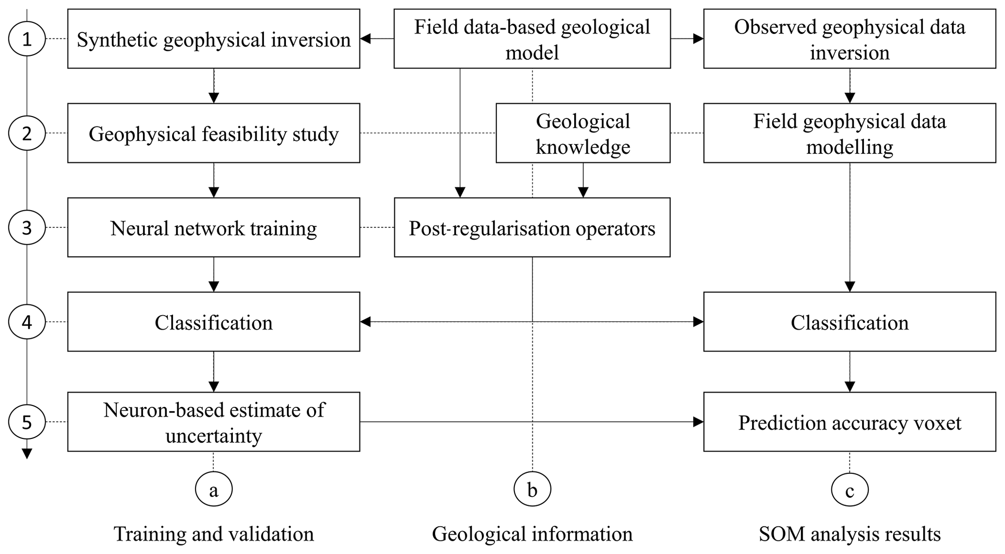
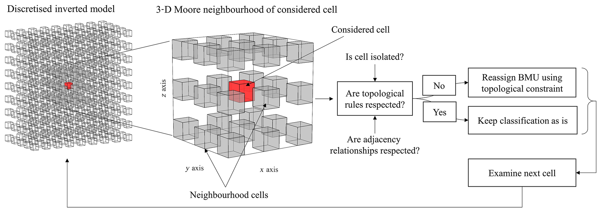
The first part of the condition in Eq. (4) is enforced using morphological closing where isolated lithologies are replaced by the most prevalent one in their neighbourhood (see Benavent et al., 2012; Ackora-Prah et al., 2015). In such cases, the BMU is updated as follows. Isolated cells (in terms of their lithology) are identified through examination of the 26-cell 3-D cubic Moore neighbourhood U of every model cell. A cell is considered isolated if, and only if, at least 25 cells of U have a lithology that differs from it. Once such a cell is identified, its BMU is updated using the closest neuron, ensuring continuity between adjacent cells in the neighbourhood U, where the lithology to be assigned is determined by a majority vote in U subject to adjacency conditions. These conditions are determined by geological knowledge (as explained below). This process is repeated for all locations until the lithological model stops changing. The general principle of post-regularization is illustrated in Fig. 1.

We point out that in contrast to Tarabalka et al. (2009) and Stavrakoudis et al. (2014), who used the first and second Chamfer neighbourhoods in 2-D around the considered model cell, we do not follow the same approach in 3-D. Our implementation of the extension of their approach to 3-D showed that, in our application case study, the adjustments of the recovered lithological model it imposes are detrimental to the consistency of the classification with geophysical measurements. That is, the perturbation of the corresponding geophysical response of the model it generates exceeds noise level and compromises the geophysical validity of the recovered model (see geophysical validation subsection below for more details). The same remark applies to the utilization of a mode filter with a $\mathrm{3}\times \mathrm{3}\times \mathrm{3}$ kernel.

The conditions relating to adjacency relationships forces the model to honour adjacency relationships extracted from surface geology (Burns, 1988; Thiele et al., 2016) in the recovered lithological model.

We determine lithological topology by identifying the contacts between adjacent model cells and represent the topological signature of lithological models using the adjacency representation of Godsil and Royle (2001). Let the adjacency matrix M of a given cell be defined as

$$\begin{array}{}\text{(5)}& M_{i>j,j}=n_{ij},M_{i\le j,j}=\mathrm{0},\end{array}$$

where n_ij is the number of contacts between lithologies i and j. Similarly, geological laws and knowledge allow the derivation of a matrix M^f defined as follows:

$$\begin{array}{}\text{(6)}& \left\{\begin{array}{ll}{M}_{i>j,j}^f=\mathrm{1}& \text{if contact between}i\text{and}\\ & j\text{contradicts geology}.\\ M_{i>j,j}^f=\mathrm{0}& \text{otherwise}.\end{array}\right.\end{array}$$

From there, it is straightforward to identify occurrences of forbidden contacts by calculating M_k⋅M^f. Therefore, ${\mathrm{1}}^{\mathbf{T}}{\mathbf{M}}_k\cdot {\mathbf{M}}^f\mathrm{1}=\mathrm{0}$ (Eq. 4) indicates that no contact violating the condition imposed by M^f is observed. The last condition in Eq. (4) can be used to prevent the local stratigraphy (in the Moore neighbourhood U of the considered cell) from violating geological rules such as “lithology B must be in conformable sequence between lithologies A and C”.

After identification of configurations forbidden by the conditions set in Eq. (4), its BMU is updated using the closest neuron honouring the set of conditions (Fig. 2, box 4a).

The next stage of the methodology we introduce is the calculation of the apportionment of each neuron in terms of the lithologies of the testing data vectors (from the synthetic survey) they predict (Fig. 2, box 5a). For instance, in a two-lithology scenario, a given node may be found to predict lithology A using the validation dataset correctly 80 % of the time (80 % accuracy) and lithology B correctly 20 % of the time (20 % accuracy). This process is described below.

The methodology is summarized in Fig. 2.

2.4 Uncertainty analysis

2.4.1 Prediction accuracy of the recovered lithologies

The prediction accuracy τ_i of lithology $i\mathit{ϵ}[\mathrm{1},\mathrm{\dots },n_{\mathrm{l}}]$ (with n_l the total number of lithologies) is the ratio of correct predictions to the total number of predictions. It is obtained from the “matching matrix” of the recovered lithologies M^c. We remind that the “matching matrix” (or “confusion matrix” in supervised learning) is a matrical representation of the number of occurrences of true/false positives/negatives.

We use the prediction accuracy τ_i as a metric measuring the capability of the node i of the trained SOM to recover lithologies. Let τ_i be expressed as

$$\begin{array}{}\text{(7)}& {\mathit{\tau }}_i={\displaystyle \frac{M_{ii}^c}{M_{ii}^c+{\sum }_{\begin{array}{l}j\ne i\\ j=\mathrm{1}\end{array}}^{n_{\mathrm{l}}}{M}_{ij}^c}},\end{array}$$

which is a particular case of the overall accuracy τ:

$$\begin{array}{}\text{(8)}& \mathit{\tau }={\displaystyle \frac{{\sum }_{i=\mathrm{1}}^{n_{\mathrm{l}}}{M}_{ii}^c}{{\sum }_{i=\mathrm{1}}^{n_{\mathrm{l}}}{\sum }_{j=\mathrm{1}}^{n_{\mathrm{l}}}{M}_{ij}^c}}.\end{array}$$

From Eq. (7), it appears that τ_i is equivalent to the frequentist probability of the ith lithology over the entire SOM. When considering a specific node j, it becomes the relative frequentist probability of the lithology i for cells classified as having the jth node as their BMU, noted τ_ij.

Figure 3 (a) Geological map of the area and (b) complete Bouguer anomaly (reproduced from Giraud et al., 2019a). The dashed red line outlines the modelled area. Capital letters “A”, “B” and “C” symbolize the possible outlines for the greenstone belts in the area.

2.4.2 Geophysical consistency

The consistency of the classification performed using SOM after application of post-regularization with field geophysical measurements might be altered by both the classification itself and by post-regularization. It is therefore necessary to ensure that the approximation of the dataset by values from the units of SOM is consistent with geophysical measurements. To this end, we verify that the geophysical response of the density contrast model m_SOM corresponding to the BMUs of each cell in the studied area fits the field measurement d within a certain tolerance assumed to approximate noise level. Consequently, we ensure that the difference between m_inv and m_SOM, $\mathrm{\Delta }m=m_{\mathrm{inv}}-m_{\mathrm{SOM}}$, satisfies the following condition:

$$\begin{array}{}\text{(9)}& \begin{array}{rl}& {∥{\mathbf{W}}_{\mathrm{d}}\left(\left(d-g\left(m_{\mathrm{inv}}\right)\right)-\left(d-g\left(m_{\mathrm{SOM}}\right)\right)\right)∥}_{\mathrm{2}}^{\mathrm{2}}\\ & ={∥{\mathbf{W}}_{\mathrm{d}}\mathbf{G}\mathrm{\Delta }m∥}_{\mathrm{2}}^{\mathrm{2}}\le \mathrm{tol},\end{array}\end{array}$$

where tol is the threshold depending on noise levels in the data above which m_inv and m_SOM are not considered geophysically equivalent.

The implication of Eq. (9) is that the difference Δm belongs to the null space of the inverse problem considered. The null space is characteristic of geophysical inversion's non-uniqueness. It is defined as the ensemble of models that reproduce geophysical data with a comparable misfit. The models honouring Eq. (9) can therefore be considered equivalent from a geophysical data point of view (Muñoz and Rath, 2006; Chen et al., 2007; Deal and Nolet, 1996). For qualitative assessment of geophysical consistency, we complement the utilization of Eq. (9) with the visual comparison of data misfit maps corresponding to the model corresponding to m_inv and m_SOM.

3 Application case: Yerrida Basin

3.1 Survey setting

This subsection introduces and summarizes the geological and geophysical context of the application case presented here. More details about the geology of the area and the initial geophysical inversion can be found in Giraud et al. (2019a) and Lindsay et al. (2018, 2020).

3.1.1 Geological and geophysical setting

The Paleoproterozoic Yerrida Basin is located in the southern part of the Capricorn Orogen (WA) and covers approximately 150 km N–S and 180 km E–W (Pirajno and Adamides, 2000) (Fig. 3a). The structures of interest in this work are Archean greenstone belts (Fig. 3), as they are prospective for Au and Ni and underlie the younger basin rocks. The basement to the Yerrida Basin is considered to be Archean granite–gneiss or greenstone rocks of the Yilgarn Craton. Lithospheric extension initiated the formation of the Yerrida Basin at approximately 2200 to 1990 Ma with deposition of the Windplain Group (Occhipinti et al., 2017; Pirajno and Adamides, 2000). The Goodin Inlier remains exposed in the central part of the basin and is in unconformable contact with the Windplain Group. A hiatus ensued, followed by deposition of the younger Mooloogool Group, which was then overlain in the east by the Tooloo Group of the Earaheedy Basin.

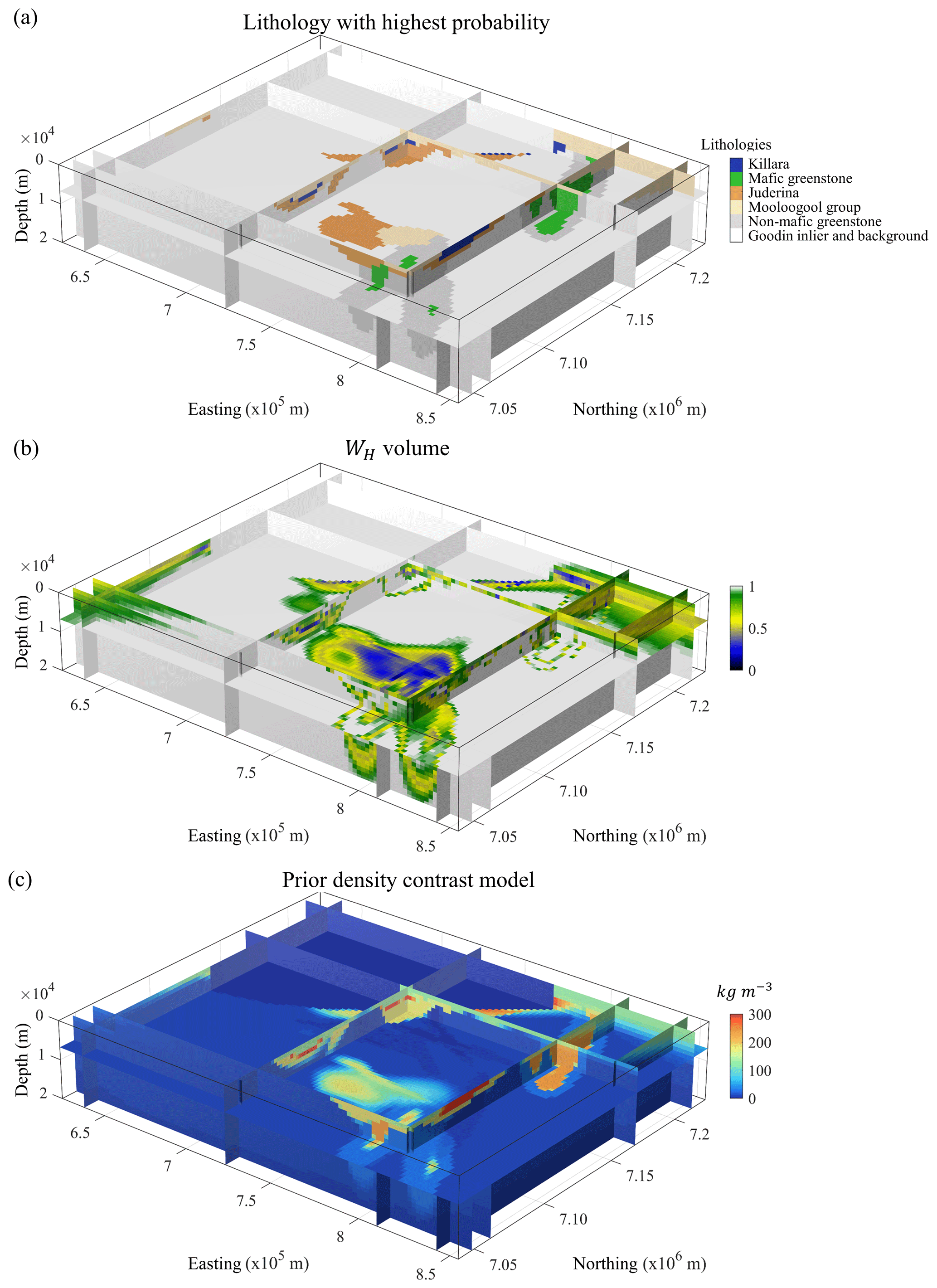
Figure 4 Prior geological modelling. Preferred lithology volume (a), geological uncertainty volume (b) and starting density contrast model (c). Modified from Giraud et al. (2019a).

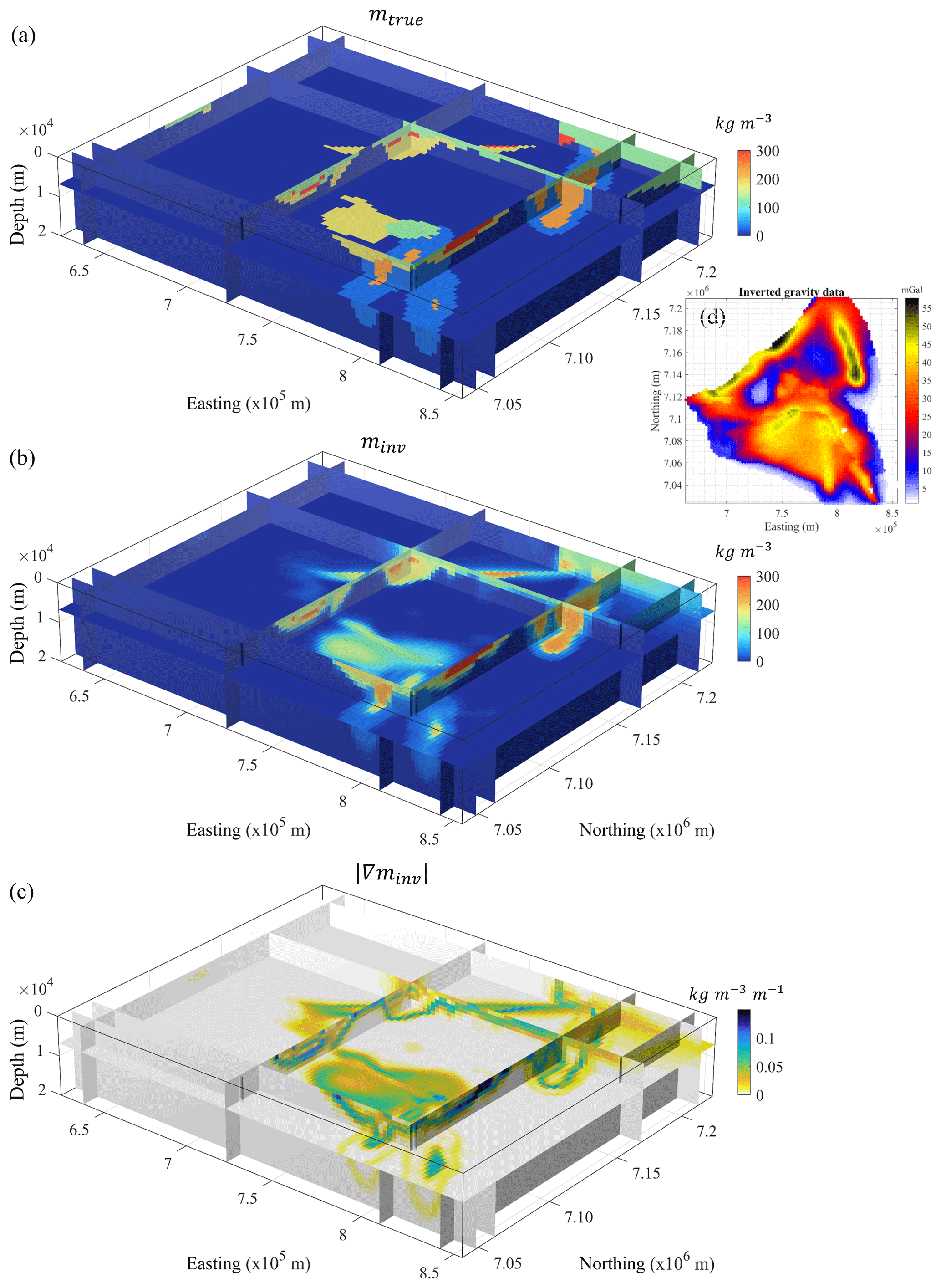
Figure 5 True density contrast model for calculation of synthetic geophysical data (a), inverted model obtained from geophysical inversion of synthetic geophysical data (b), corresponding spatial gradient of density contrast (c) and synthetic geophysical data (d).

The density contrast of the lithologies observed in the area ranges between 0 and 330 kg m⁻³, making it appropriate for gravity modelling and inversion (Giraud et al., 2019a; Lindsay et al., 2018). While basin rocks exhibit some density contrast, the greenstone is conspicuous in gravity data with a density contrast expected to lie between 190 and 270 kg m⁻³, making it an attractive subject for gravity inversion. Field geological measurements (orientation data in the form of interfaces and foliations) and petrophysical data were used to build the reference geological model. Airborne geophysical data, Landsat and Aster 8 satellite data were also used to support the interpretation of geological measurements.

The gravity anomaly dataset we consider (Fig. 3b) is comprised of a total of 4882 measurement points. The model is discretized into $\mathrm{100}\times \mathrm{100}\times \mathrm{42}$ cells of dimensions 2.335 km × 1.875 km × 1.0475 km down to approximately 44 km depth. Weights and parameters used for the inversion of synthetic data follow the settings of Giraud et al. (2019a) on field data.

3.1.2 Geological modelling and synthetic geophysical survey

This subsection introduces the semi-synthetic survey we performed for the training of SOM.

The volumes of most probable lithology, W_S and the starting model are shown in Fig. 4. Volumes shown in Fig. 4a, b and c are used for the training and validation dataset for SOM training as explained in Sect. 2.2.

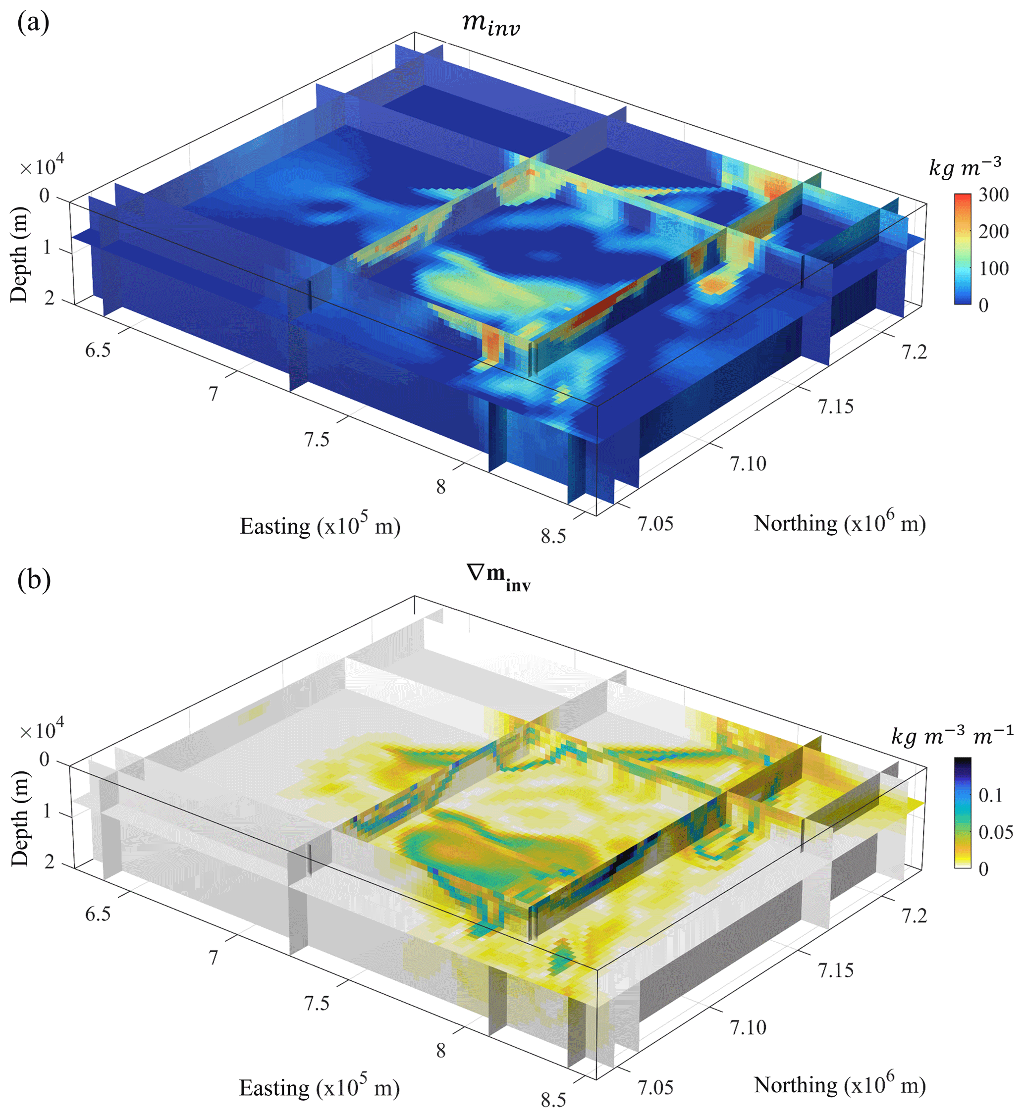
Figure 6 Inverted model obtained from geophysical inversion of field geophysical data (a) and corresponding spatial gradient of density contrast (b).

We use the modelling results shown in Fig. 4 to calculate a synthetic geophysical dataset (Fig. 5d). The model used to generate the synthetic geophysical measurements is shown in Fig. 5a. The corresponding inverted model and its gradients are shown in Fig. 5b and c. Volumes shown in Fig. 5b and c are used for training and validation.

3.1.3 Field geophysical data inversion

The density contrast model obtained from inversion of field geophysical data and its gradients are shown in Fig. 6a and b. Visual comparison of inverted models shown in Figs. 6a and 5b reveals that mesoscale structures are similar with the exception of large structures presenting low-density contrasts at depth (darker shades of blue in Fig. 6a). This is reflected in Fig. 6b, which exhibits low gradient values in these areas.

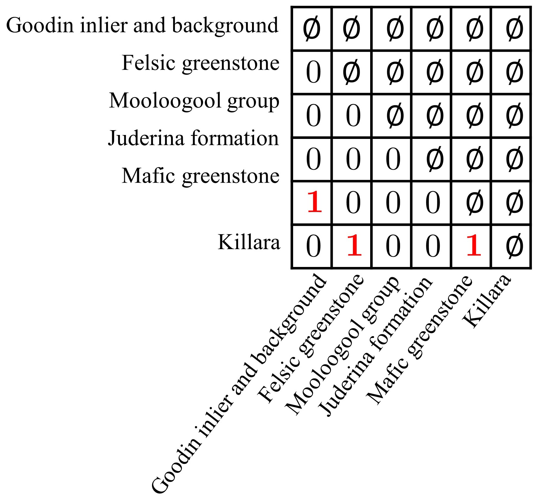
Figure 7 Matrix defining forbidden contact between lithologies in the Yerrida Basin. Here, 1 means that two units may be in contact with each other, 0 means that they may not, and φ represents symmetric relationships or when the same unit is adjacent to itself (which geologically may occur across a fault but cannot be resolved by the geophysical data available).

Figure 8 (a) Elbow curve of the quantization error for the determination of the optimum number of neurons (or units) in SOM and (b) prediction accuracy for the different lithologies present in the training and validation datasets. Note that after 750 units, the quantization error for the different lithologies stabilizes and oscillates around its maximum values.

The classification of lithologies using SOM is performed applying the trained network to volumes shown in Figs. 4b, c and 6a, b. The next subsections describe the geological laws used for post-regularization (Sect. 3.1.4) and the classification process (Sect. 3.2.2).

3.1.4 Geological rules for post-regularization

As mentioned above, for clarity in this demonstration, only adjacency relationships are considered. The utilization of simple relationships such as adjacency is also chosen because in areas of sparse data, a full description of geological rules (fault relationships with fault and stratigraphy) is often not known. Given the complexity of the Yerrida Basin and its magmatic and deformation history, several base geological rules can be derived to assess the plausibility of recovered lithological models. Using fundamental geological principles (such as uniformitarianism, superposition, Walther's law, cross-cutting relationships and original horizontality), the two most likely restrictive adjacency rules are as follows. We assume that the mafic greenstone bodies cannot be in contact with the Killara Formation (in the Mooloogool Group) since our field data suggest that the Killara Formation is a volcanic unit that is restricted to the Yerrida Basin and thus not in contact with the mafic greenstone. In addition, we assume that the mafic greenstone cannot be in contact with the Goodin Inlier and background (or basement), as the mafic greenstone is modelled to be enveloped by the felsic component of the greenstone.

The matrix M^f defining the contacts forbidden by geology as described above is given in Fig. 7.

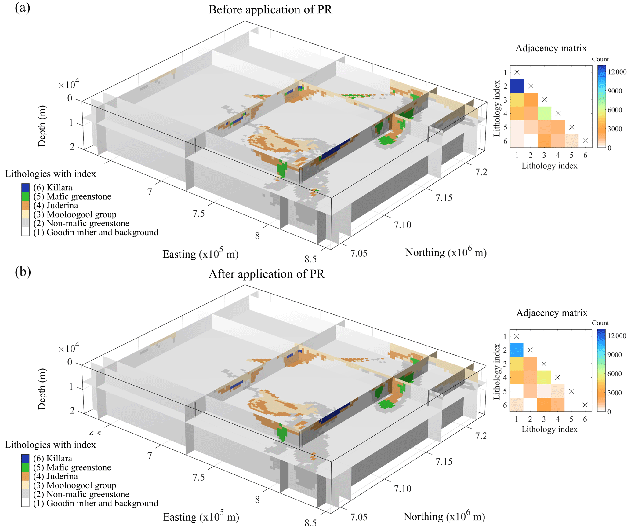
Figure 9 Recovered lithologies before post-regularization (a) and after (b) next to the corresponding adjacency matrix (right-hand side). The indices used to designate lithologies are indicated in the legend of the volume (left-hand side).

3.2 Geologically constrained SOM classification and uncertainty analysis

3.2.1 Training the neural network

In this work, we use approximately 500 neurons (units) for the training of SOM. This number is inferred from the analysis of the elbow curve we calculated using the validation datasets (see Fig. 8) and approximately matches the proposed value of $\mathrm{5}\sqrt{N}$ (with N the total number of observation) proposed by Vesanto and Alhoniemi (2000) and commonly used since (Shalaginov and Franke, 2015). The chosen number of units is corroborated by the lithology prediction accuracy (Fig. 8) as approximating the point of diminishing returns, i.e. the number of nodes beyond which additional nodes are becoming nearly redundant.

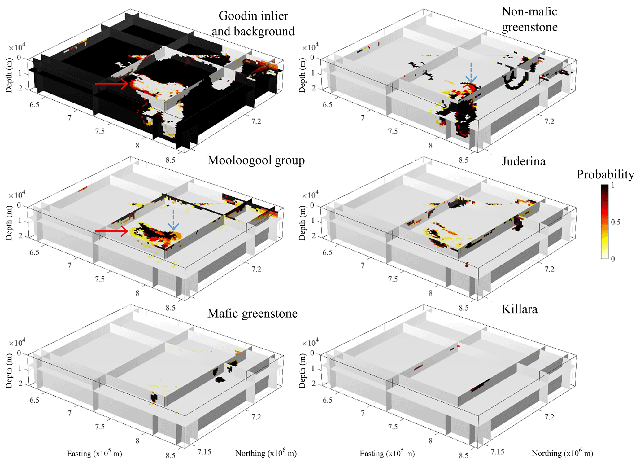
Figure 10 Frequentist probability volumes of recovered lithologies calculated as per Eq. (3). The arrows are drawn to support interpretation.

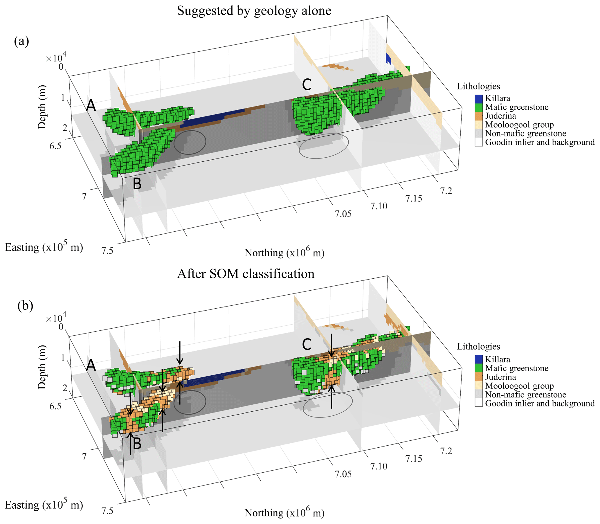
Figure 11 Mafic greenstone belts and their surroundings following geological modelling only (a) and after SOM classification (b). The cells shows in panels (a) and (b) have the same geographical location and are coloured according to lithology. The vertical arrows show areas where mafic greenstone is thinner than suggested by geology only. The elliptical shapes shows zones where expected non-mafic greenstone is replaced by the background lithology.

The trained map presents a mean quantization Q equal to 0.075, which indicates relatively good approximation of the datasets by the trained SOM. This is illustrated by Fig. 8, where all lithologies are recovered with a prediction accuracy superior to 90 %.

3.2.2 Classification and post-regularization

After classification of the recovered model, we performed post-regularization to remove geologically unrealistic features from the classified lithological volume. Figure 9 shows the classification results before and after post-regularization, along with the associated adjacency matrix.

As can be inferred from the adjacency matrices plotted in Fig. 9, the number of contacts between units with indices 1 and 2, respectively, is reduced by the application of post-regularization. One reason for this is the presence of a number of inclusions of lithology 1 in lithology 2, and vice versa; a total of 2561 such inclusions was identified. Overall, the number of contacts between lithologies 5 and 2 increased slightly due to post-regularization because a large percentage of contacts between lithologies 5 and 1 has been reassigned as contacts between lithologies 5 and 2. The elimination of contacts between lithologies 5 and 6 is also visible in Fig. 9.

3.2.3 Estimated confidence in recovered lithologies

For each node of the SOM, we calculate the prediction accuracy τ_i (Eq. 3) for the different lithologies observed in the area using the cross-validation dataset. After application of the trained SOM for the classification of inversion results obtained from the inversion of field geophysical data, we obtain a frequentist probability volume for each lithology. Figure 10 shows the resulting frequentist probability volumes for the six lithologies present in the Yerrida Basin.

Figure 10 exhibits probabilities between 0.3 and 0.6 in the area marked by the two arrows. This suggests that these zones are the least well constrained. Note that from Fig. 10, we can interpret the presence of mafic greenstone with confidence, as it shows high frequentist probability nearly everywhere classification suggests its presence. For completeness, assessment of the prediction accuracy of the different lithologies is shown by the corresponding box plot in Appendix B.

3.2.4 Geophysical null space validation and implications for geological interpretation

Applying Eq. (9), we obtain ${∥W_{\mathrm{d}}\mathbf{G}\mathrm{\Delta }m∥}_{\mathrm{2}}^{\mathrm{2}}=\mathrm{6}\times {\mathrm{10}}^{-\mathrm{4}}$, indicating that the model can be considered geophysically equivalent overall. This is illustrated by the map of the corresponding data misfits (see Fig. B1 in Appendix B), which indicates that we can consider the recovered lithological model after application of post-regularization as reflective of both geophysical and geological information. Focusing on the mafic greenstone belts of interest in the area (Fig. 11), the classification results allow us to propose the following geological interpretations.

Figure 11 shows that the northern portion of the greenstone belts A and B recovered by geophysical inversion and SOM classification is thinner in their northern part than was proposed by the initial geological model. Likewise, greenstone belt C seems to be much thinner near its centre than expected. Given the data density and lack of understanding we have about the depth of this greenstone belt, this observation is plausible. It confirms and refines considerably the crude, preliminary lithology differentiation of Giraud et al. (2019a) that was based only on density contrast value. The cause of the thinning of mafic greenstone belt C could be attributed to faulting, folding or the topography of the palaeoenvironment where the protoliths to the belt were formed, which are not captured directly by surface geology. The portion of the southern Merrie Greenstone Belt (mafic greenstone C) is shown to be thinner than expected, prompting a review of the structure of existing models. A plausible reason is the presence of structure that has not been identified from the initial interpretation of geophysical data. In addition, the potential presence of deep-penetrating faults or shear zones, as shown in Fig. 11b by the arrows around greenstone C, hints at a possible false assumption that the Merrie Greenstone Belt is a single and coherent geological body.

4 Discussion

The application of the technique presented here is not restricted to usage of the particular geophysical or geological modelling schemes generating the modelling inputs to this study. The methodology we introduced is general and any different stand-alone geophysical and geological modelling schemes could also be used.

The work presented here relied on SOM, which can be seen as an extension of the k-means and c-means clustering algorithms used for lithological differentiation (Paasche and Tronicke, 2007; Carter-McAuslan et al., 2015; Sun and Li, 2015, 2016; Maag and Li, 2018; Ward et al., 2014; Singh and Sharma, 2018), with which it shares a number of characteristics. We can therefore assume that our findings may hold true for these techniques.

We have shown that the utilization of post-regularization can be effective for increasing geological realism in the recovered lithological models while preserving the geophysical validity of the corresponding model. The geological principles we used to design our post-regularization operator apply to lithological topology and focus on the adjacency relationship between cells. Ideally, post-regularization should also consider the surface area of contacts and their topology. This could be followed by, for instance, a 3-D extension of the geological model-editing approach of Anquez et al. (2019) to produce genuine geological models honouring age relationships, stratigraphic principles, etc. Provided that the resulting models honour Eq. (9), this approach would ensure that while they are geophysically valid, they can be readily used for interpretation or by commercial or non-commercial geological modelling engines, reservoir simulations, etc. without further processing.

We also believe that post-regularization can be successfully applied to other clustering techniques. In addition, the implementation of post-regularization presented here can be readily applied to existing classification, regardless of the classification algorithm used, as it only adjusts the classification using spatial–contextual features in the classified model and could assist the geological characterization of inversion results (Melo et al., 2017).

The example we have shown uses a covariance matrix W_s (Eq. 1) that results from geological modelling. It is used as a proxy for the uncertainty about our knowledge in terms of structural geology. Such prior information could also be derived from techniques other than geological modelling such as prior geophysical modelling, be it using the same or different geophysical methods. While we do not address the uncertainty in the density model directly, we assume that non-uniqueness and measurement uncertainty affect both field data and synthetic data in the same manner due to the noise component and parameterization of each being the same.

An important result produced here involves the identification of regions which do not adequately conform to the initial model parameters (Fig. 11). While this issue remains unresolved, the capability of our method to identify problematic regions is useful to drive reinterpretation of data, consideration of additional models and, eventually, increased geological knowledge of the target.

Future work may include the generation of multiple lithological models using the trained SOM and the frequentist probability volume associated with it. By selecting models belonging to the null space of the geophysical data (i.e. satisfying Eq. 9), we expect that this would allow the identification of a series of a few archetypes that would be representative of the various datasets used in the geoscientific modelling workflow.

5 Conclusions

We have introduced a post-inversion classification technique relying on SOM that enables the recovery of lithologies, the corresponding frequentist probability voxet thereby remediating to some of the limitations of deterministic inversion. The proposed technique utilizes a post-regularization scheme enforcing elementary geological principles to the recovered lithological model while maintaining geophysical validity. We have applied this new methodology to the Yerrida Basin (Western Australia) and shown how it improves the geological plausibility of the recovered model. Results allowed us to confirm previous results and bring new insights into possible reinterpretation of the geometry of prospective greenstone belts.

Appendix A: Data misfit generated by SOM classification and post-regularization

In Fig. A1, data misfit and the absolute data misfit difference (Fig. A1b and c, respectively) show values which, in places, are relatively high but which are in line with the gravity data inversions. Figure A1a and b show similar features to the exception of a patch in the central part of the model (northing $\sim \mathrm{7.09}\times {\mathrm{10}}^{\mathrm{6}}$ m – easting $\sim \mathrm{7.7}\times {\mathrm{10}}^{\mathrm{5}}$ m), where Fig. A1b shows values that are approximately 1.5 mGal higher. Figure A1c shows misfit differences generally on the order of, or lower than, 2 mGal. Also note that there are places where Fig. A1b shows lower misfit than Fig. A1a.

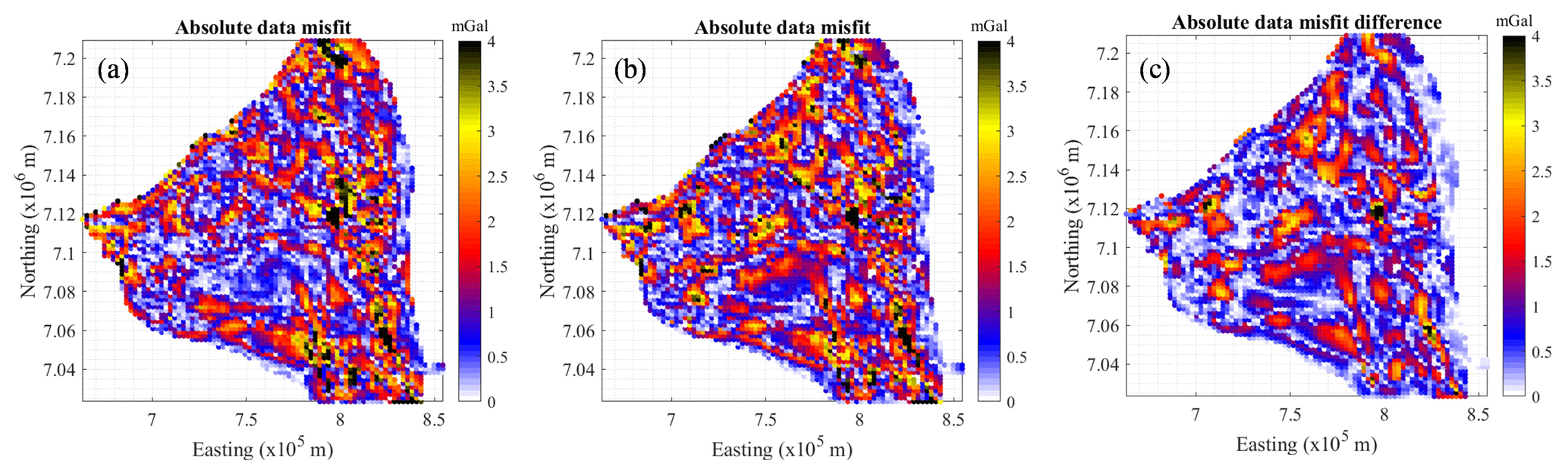
Figure A1 (a) Comparison of absolute data misfit maps obtained for the inverse model used here (reproduced from Giraud et al., 2019a) and (b) after post-regularization, with (c) the misfit differences between panels (a) and (b).

Appendix B: Data misfit generated by SOM classification and post-regularization

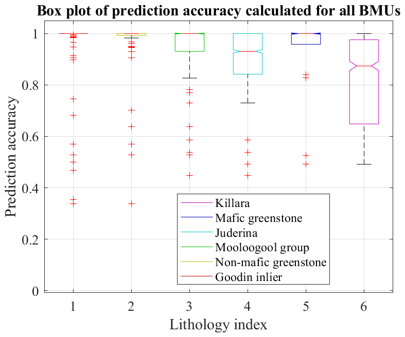
Figure B1 Box plot of prediction accuracies for the different lithologies. Red crosses mark outliers.