the Creative Commons Attribution 4.0 License.
the Creative Commons Attribution 4.0 License.
 | 07 May 2020
Magnetic properties of pseudotachylytes from western Jämtland, central Swedish Caledonides
Bjarne S. G. Almqvist
Hagen Bender
Amanda Bergman
Uwe Ring
Fault kinematics can provide information on the relationship and assembly of tectonic units in an orogen. Magnetic fabric studies of faults where pseudotachylytes form have recently been used to determine direction and sense of seismic slip in prehistoric earthquakes. Here we apply this methodology to study magnetic fabrics of pseudotachylytes in field structures of the Köli Nappe Complex (central Swedish Caledonides), with the aim to determine fault kinematics and decipher the role of seismic faulting in the assembly of the Caledonian nappe pile. Because the pseudotachylyte veins are thin, we focused on small (ca. 0.2 to 0.03 cm3) samples for measuring the anisotropy of magnetic susceptibility. The small sample size challenges conventional use of magnetic anisotropy and results acquired from such small specimens demand cautious interpretation. Importantly, we find that magnetic fabric results show inverse proportionality among specimen size, degree of magnetic anisotropy and mean magnetic susceptibility, which is most likely an analytical artifact related to instrument sensitivity and small sample dimensions. In general, however, it is shown that the principal axes of magnetic susceptibility correspond to the orientation of foliation and lineation, where the maximum susceptibility (k1) is parallel to the mineral lineation, and the minimum susceptibility (k3) is dominantly oriented normal to schistosity. Furthermore, the studied pseudotachylytes develop distinct magnetic properties. Pristine pseudotachylytes preserve a signal of ferrimagnetic magnetite that likely formed during faulting. In contrast, portions of the pseudotachylytes have altered, with a tendency of magnetite to break down to form chlorite. Despite magnetite breakdown, the altered pseudotachylyte mean magnetic susceptibility is nearly twice that of altered pseudotachylyte, likely originating from the Fe-rich chlorite, as implied by temperature-dependent susceptibility measurements and thin-section observations. Analysis of structural and magnetic fabric data indicates that seismic faulting occurred during exhumation into the upper crust, but these data yield no kinematic information on the direction and sense of seismic slip. Additionally, the combined structural field and magnetic fabric data suggest that seismic faulting was postdated by brittle E–W extensional deformation along steep normal faults. Although the objective of finding kinematic indicators for the faulting was not fully achieved, we believe that the results from this study may help guide future studies of magnetic anisotropy with small specimens (<1 cm3), as well as in the interpretation of magnetic properties of pseudotachylytes.
- Article
(22153 KB) - Full-text XML
- BibTeX
- EndNote


Pseudotachylytes are fault rocks that represent quenched frictional melts generated during coseismic slip (Magloughlin and Spray, 1992; Sibson, 1975). Pseudotachylytes have been documented in fault zones within the Köli Nappe Complex, central Sweden (Beckholmen, 1982). Since the discovery of these localities almost 4 decades ago, understanding of pseudotachylyte generation has improved fundamentally (Lin, 2008; Rowe and Griffith, 2015). For example, pseudotachylyte characteristics have been used to infer dynamics of seismic faulting (e.g., Di Toro et al., 2005). A recently developed approach exploits magnetic properties and anisotropy of magnetic susceptibility of pseudotachylytes for deducing the focal mechanism of ancient earthquakes (Ferré et al., 2015). In an attempt to find the kinematics of a ductile-to-brittle shear zone in the Köli Nappe Complex, we adopted this method to the pseudotachylytes in the Köli Nappe Complex. Information about fault kinematics could offer evidence for nappe stacking dynamics along this shear zone within the Köli Nappe Complex (e.g., Bender et al., 2018). Additionally, the pseudotachylyte data can be compared to kinematic data from late- and post-orogenic extensional faults that crosscut the nappe architecture (Bergman and Sjöström, 1997; Gee et al., 1994), which is important to understand the relationship between the top-W shear sense late-orogenic extensional phase and brittle deformation related to pseudotachylyte formation. It is found that the magnetic fabric reflects the petrofabric, but it does not reveal the direction or sense of seismic slip. Observations made on the magnetic properties of pseudotachylytes reveal differences in bulk susceptibility of altered and pristine pseudotachylytes. An additional insight provided in this work is that magnetic fabric studies that use small-to-very-small sample sizes (i.e., 0.2 to 0.03 cm3) need to be carefully considered given potential measurement-related artifacts.
1.1 Rock magnetism and its application to pseudotachylytes
Frictional melting significantly affects magnetic properties of fault rocks. The newly crystallized mineral assemblage of pseudotachylytes is distinctly different from that of its host rock (Ferré et al., 2012). The rapid quenching leads to a remanent magnetization, which is acquired coseismically but sometimes contains post-seismic superimposed magnetizations, and hence impacts interpretation of paleomagnetism (Ferré et al., 2014; Fukuchi, 2003). Anisotropy of magnetic susceptibility of pseudotachylytes may also record information about the viscous flow of the friction melt (Ferré et al., 2015; Scott and Spray, 1999). Comparison of fault plane geometry and orientation with the magnetic fabric and petrofabric has been used to deduce earthquake kinematics and focal mechanism (Ferré et al., 2015).
The magnetic fabric of a rock is defined by its anisotropy of magnetic susceptibility (AMS), which in turn reflects the sum of individual magnetic responses of the rock-forming minerals (Borradaile, 1987). To use magnetic fabrics for inferring flow direction and sense, the carriers of rock magnetism must be known (Cañón-Tapia and Castro, 2004). In general, minerals respond in three fundamental ways to applied magnetic fields: diamagnetic, paramagnetic or ferromagnetic sensu lato (Butler, 1992; Tauxe, 2010). Depending on which of these behaviors is dominant in a rock specimen, AMS needs to be interpreted in different ways. Low susceptibility of diamagnetic minerals generally makes them subordinate contributors to the bulk rock AMS (Hirt and Almqvist, 2012, and references therein). Most rock-forming minerals are paramagnetic, for which AMS is foremost controlled by crystallography. AMS in paramagnetically dominated rocks reflects the crystallographic preferred orientations of these minerals (Hirt and Almqvist, 2012). However, pseudotachylytes have been shown to contain authigenic magnetite produced during frictional melting (Nakamura et al., 2002). For ferromagnetic minerals, AMS is mainly controlled by grain shape and orientation distribution, with the most notable exception of hematite (Borradaile and Jackson, 2010). With few exceptions, paramagnetic and ferromagnetic minerals express normal AMS fabrics. In such fabrics, the longest grain dimensions coincide with the maximum principal AMS axes (Tarling and Hrouda, 1993). For these cases, the flow direction can be deduced from the magnetic lineation (e.g., Ernst and Baragar, 1992).
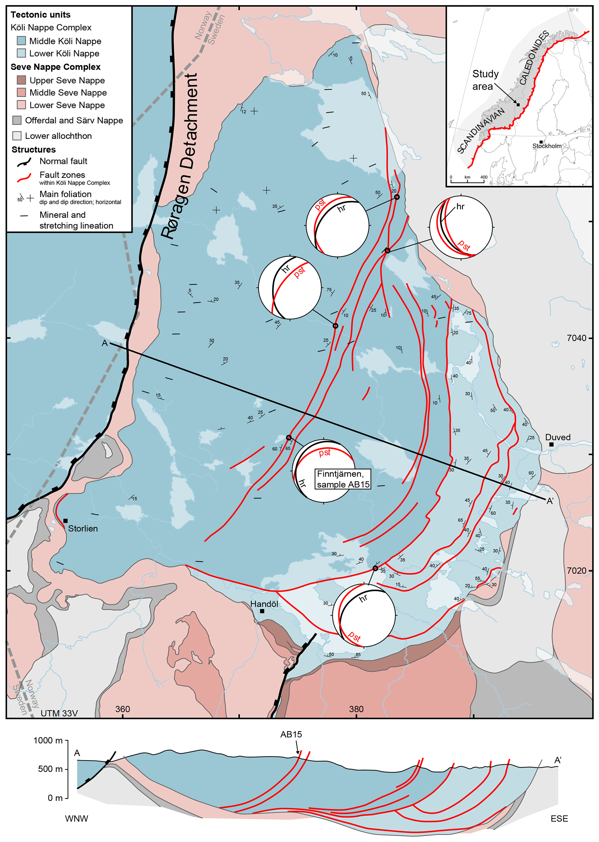
Figure 1Geological map of the Tännforsen Synform and section A–A' across it (modified after Beckholmen, 1984). Structural positions of tectonic units are indicated in the top left. Structurally lower faults are truncated by structurally higher faults within and beneath the Köli Nappe Complex. Lower-hemisphere equal-area nets show orientations of host rock schistosity (hr) subparallel to pseudotachylyte-bearing fault veins (pst) (data from this study and Bergman, 2017). The Røragen Detachment in the west cuts across all other units beneath it, illustrating that it developed structurally the latest.
In western Jämtland, the Köli Nappe Complex mainly consists of greenschist- to amphibolite-grade metavolcanic and metasedimentary rocks exposed in the Tännforsen Synform (Fig. 1; Beckholmen, 1984). Mineral and stretching lineations trend E–W to SE–NW. Foliations dip shallowly and their strike generally conforms to the shape of the synform. Several minor and two major fault zones separate the thrust sheets of the Köli Nappe Complex. The fault zones show ductile to brittle structures that are associated with pseudotachylytes (Beckholmen, 1982). We investigated the structurally highest of these fault zones, the Finntjärnen fault zone (Fig. 1). The Köli Nappe Complex and its underlying units are crosscut by the Røragen Detachment and associated brittle W-dipping normal faults (Bergman and Sjöström, 1997; Fig. 1; Gee et al., 1994). At Finntjärnen (latitude and longitude coordinates: 63.389350 ∘N, 12.480276 ∘E), the schistosity of the micaschist host rock dips shallowly to the WNW (overall host rock schistosity S 302∕15, Fig. 2a). Mineral and stretching lineations are shown by the orientation of biotite and boudinaged amphibole crystals in the foliation plane, and they plunge shallowly to the W (overall host rock lineation L 262∕08, Fig. 2a). Mylonitic shear sense indicators associated with the ductile fabric were not observed, although top-ESE shear sense indicators in mylonites were mapped regionally by Bender et al. (2018, 2019) in the middle and lower Köli nappe. Fault veins commonly occur as foliation-parallel generation veins and crosscutting injection veins (Figs. 2a, 3).
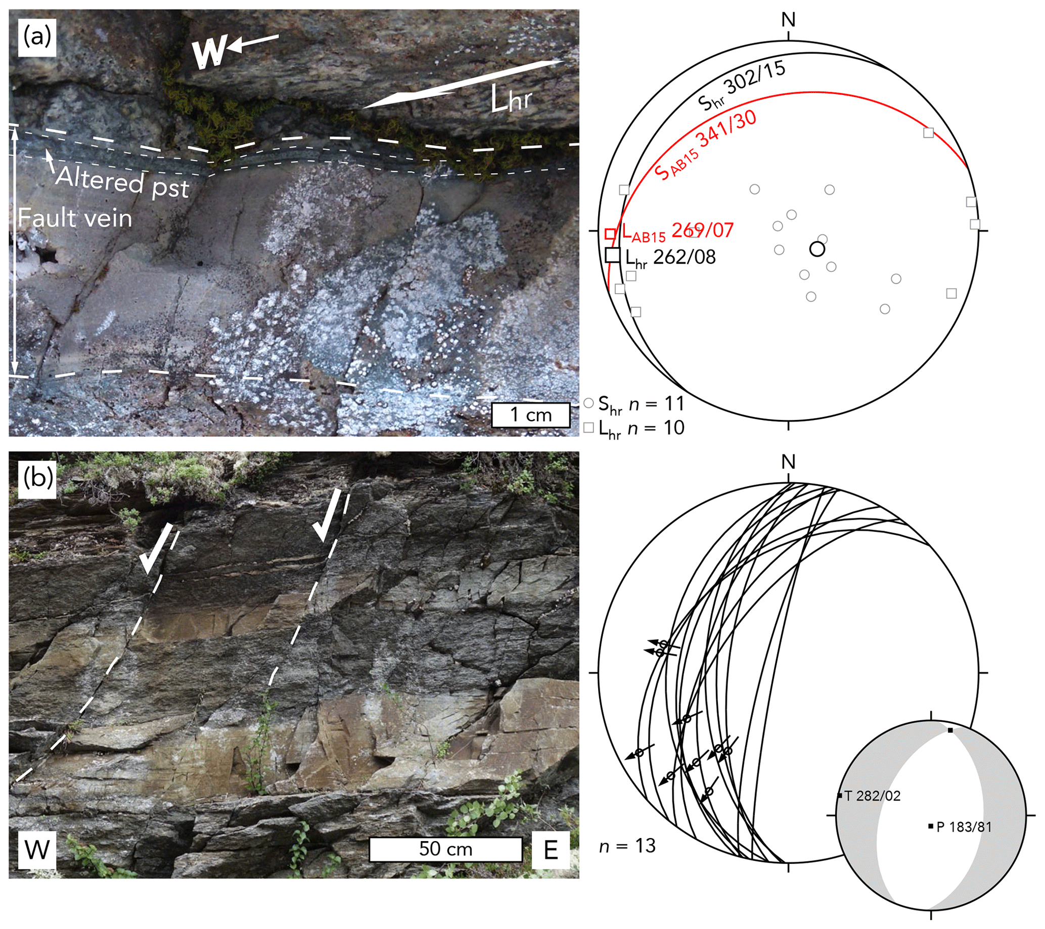
Figure 2(a) Field photograph of the microstructurally investigated fault vein. It is 3 cm wide, foliation-parallel and exhibits a 5 mm thick band of bluish, altered pseudotachylyte at its top. Note the crosscutting, steeply dipping fractures. Equal-area projections with poles to host rock schistosity planes (Shr), host rock lineations (Lhr) and orientation of the investigated sample AB15 (red great circle). Mean orientations for Shr and Lhr are indicated with large symbols. (b) Brittle, steeply W-dipping normal faults crosscut the ductile fabric. Sense of slip is indicated by calcite slickenfibers on some of the fault planes. Fault plane solution for these faults (b) shows E–W extension (data processed with FaultKin 7; Marrett and Allmendinger, 1990).
The fault veins contain both pseudotachylyte and subordinate ultracataclasite. Macroscopically, four different types of fault rock can be distinguished: (1) fractured host rock or protolith occurs in millimeter-to-centimeter-wide domains between brittlely undeformed host rock and fault veins. It appears very similar to the host rock, features microscopic fractures and <1 to 10 mm wide injection veins; (2) cataclasite has the same color as the host rock, but it is much finer grained and appears as patches within fault veins; and (3) pseudotachylyte, which is grouped into preserved pst and altered pst, based on the degree of alteration that the pst has experienced; pseudotachylyte being fault rock with the microstructural evidence for frictional melting. Preserved pseudotachylytes display compositional flow-banding and consist of a massive, bright gray, amorphous matrix containing <2 mm sized clasts of host rock fragments and minerals; altered pseudotachylyte is bluish-gray and massive, exhibits layer-parallel banding, and generally has sharp boundaries to unaltered pseudotachylyte (Fig. 3). On slabs cut from an oriented sample (for details, see Sect. 4.1), the coseismic slip direction cannot be deduced from fabrics in the fault vein.
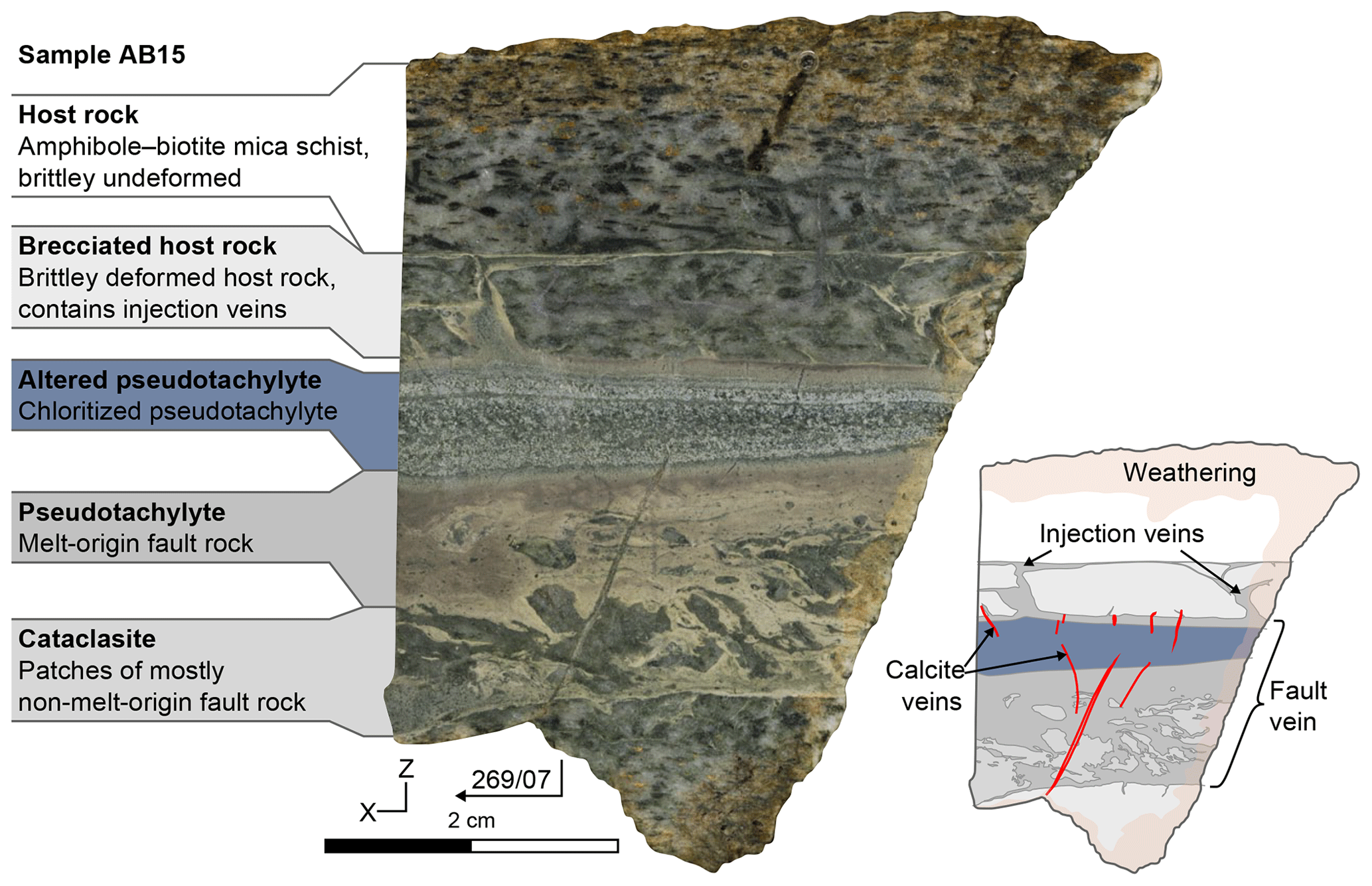
Figure 3Macroscopic appearance of sample AB15, showing the different kinds of faulted rock in the studied sample (i.e., brecciated host rock, altered pseudotachylyte, pseudotachylyte and cataclasite); characterization of fault rock types is based on microscopic observations. The inset figure shows interpreted structures in the fault. The image represents the XZ plane of the finite strain ellipsoid, where X is parallel to the stretching lineation and Z is normal to the foliation plane.
At the outcrop scale, offset schistosity planes and compositional layering in micaschist along brittle W-dipping faults commonly occur (Fig. 2b). From orientations and slip sense of these faults, P and T axes indicating E–W extension were calculated (Fig. 2b). These axes give a kinematic solution with extensional (T) and contractional (P) directions of strain (Fossen, 2010). Calcite-filled veins crosscut the ductile fabric and the fault veins (Fig. 3). The faults are likely late- or post-orogenic structures that cut across the earlier structures related to nappe emplacement.
3.1 Sample preparation
An oriented sample of a foliation-parallel fault vein with host rock on either side was collected in the field (sample AB15, schistosity 341∕30, mineral lineation LAB15 269∕07; Figs. 2 and 3). The hand specimen was cut with a diamond saw into 5 to 10 mm thick slabs parallel to the lineation and perpendicular to the foliation. A thin section was prepared from one of these slabs. The rest of the slabs were cut into lineation-parallel sticks of approximately equal width and height. From these, 116 cube-shaped specimens were cut for magnetic experiments; x axes of the cubes are parallel to Lhr and z axes are perpendicular to Shr. Due to the small spatial distribution of host or fault rock, specimen cubes are unconventionally small (side length 5.3±1.2 mm, volume 0.17±0.13 cm3; uncertainty levels here and throughout the article are 1σ) compared to standard-sized specimens (7 to 11 cm3) used in paleomagnetism (Table S1 in the Supplement). Therefore, the shape and size of cube dimensions were compared to properties of the AMS ellipsoid and uncertainties related to the cube dimension were also investigated. Despite expending particular care to avoid cutting specimens with different types of host or fault rock, specimens with mixed rock types occur. Approximate modal proportions for each rock type per specimen are presented in Table S2 in the Supplement.
3.2 Magnetic properties
3.2.1 Anisotropy of magnetic susceptibility
Anisotropy of magnetic susceptibility (AMS) was measured using a MFK1-FA susceptibility bridge (Agico, Inc.) operated at 200 A m−1 alternating current (AC) field and 976 Hz frequency. A semiautomatic sample rotation scheme was used, with manual orientation of the cubic sample in three unique positions and measurements during sample rotation, effectively yielding high-resolution measurements in the three body planes of the specimen. Orientation parameters used for data acquisition with the Safyr4W software were P1 = P3 = 6 and P2 = P4 = 0, so that specimen x-axes plunge parallel to Lhr and specimen z-axes point upward perpendicular to Shr (Safyr4W User Manual, 2011). The AMS is expressed by the orientation and magnitude of the principal axes of susceptibility . Further parameters describing AMS data include the mean susceptibility , magnetic foliation , magnetic lineation and Jelinek's parameter for the degree of anisotropy Pj (Jelinek, 1981). The shape of the susceptibility ellipsoid is described by . Only at and is the AMS ellipsoid rotational oblate and prolate, respectively. For , the AMS ellipsoid is oblate; for 0 > , it is in contrast prolate (Jelinek, 1981). Mean susceptibility km has been normalized for specimen volume. The standard error (s) of the mean susceptibility is expressed by , where S0 is the residual sum of squares given by , and N=2. The sum of squares (S) is calculated considering all measured components zi, such that
The parameter R is the reduction in sum of squares and is calculated as described by Jelinek (1996). For data visualization, specimens containing more than one host or fault rock type were plotted based on their modal composition. The specimens were assigned to the dominant host or fault rock type composing the specimen. One specimen containing three rock types and 12 specimens composed of two rock types, each with 50 % mode, were considered mixed analyses. These data are therefore only presented in the data tables and were excluded from orientation and parameter analysis of AMS data.
3.2.2 Frequency dependence of susceptibility
Frequency-dependent magnetic susceptibility was measured using a MFK1-FA susceptibility bridge (Agico, Inc.) operated at 200 A m−1 AC field and frequencies of F1=976 Hz and F3=15 616 Hz. In order to minimize the effect of anisotropy, all measurements were performed with the sample cubes oriented in the same position with their positive x axes horizontally pointing toward the operator (POS. 1 in Safyr4W User Manual, 2018; https://www.agico.com/, last access: 3 April 2020). Frequency dependence can be generally inferred when the mass-dependent susceptibility (χ; used in this study) measured at F1 is higher than F3. Frequency dependence is used to identify superparamagnetic magnetite, as a narrow grain size distribution ranging from ∼15 up to ∼30 nm, and show frequency-dependent susceptibility (Hrouda, 2011). The method was here used to help answer the question of if very fine grained magnetite (i.e., Dearing et al., 1996) formed during partial melting and recrystallization associated with the fault-slip that formed the pseudotachylyte.
3.2.3 Temperature dependence of susceptibility
Temperature dependence of magnetic susceptibility was measured using a MFK1-FA system, equipped with a CS4 furnace. Six sample cubes were analyzed individually; two sample cubes were analyzed together (AB15-13 and AB15-61) because of their small volumes. The samples were ground to a powder with an agate mortar, being careful not to contaminate the sample with outside iron particles or magnetic phases from other materials. Magnetic susceptibility measurements at 200 A m−1 AC field and 976 Hz frequency were conducted from room temperature up to 700 ∘C and subsequently cooled back to room temperature, with a heating and cooling rate of 11.8 ∘C min−1. Specimen AB15-67 was measured in air; all other specimens in argon atmosphere. Thermomagnetic data of the empty furnace were smoothed (5-point running mean) and subtracted from the sample thermomagnetic data using the Cureval8 software (Agico, Inc.).
3.2.4 Hysteresis
Hysteresis loops were performed with a Lake Shore vibrating sample magnetometer with a maximum applied field of 1 T. Data processing was performed with the MATLAB toolbox HystLab (Paterson et al., 2018), using a linear high-field slope correction and automatic drift correction. The hysteresis data were normalized by the mass of the specimen. The extracted hysteresis parameters included saturation magnetization (Ms), saturation remanent magnetization (Mrs) and coercivity (Hc). In addition, parameters of the induced hysteretic (Mih) remanence hysteresis (Mrh) curves are presented in the results section, where the two parameters are defined as half the sum and half the difference between the upper and lower hysteresis branches, respectively (Paterson et al., 2018). The noise of the measurements is expressed by the root-mean-square (rms) noise after paramagnetic slope correction and represents the signal-to-noise ratio of the hysteresis measurements (Paterson et al., 2018).
3.3 Shear sense determination using AMS
Obliquity between shear plane and magnetic fabric may be used to determine the sense of slip. Progressive shearing rotates maximum and intermediate principal axes of strain and AMS toward the shear plane (Borradaile and Henry, 1997). Kinematics are indicated in a plane perpendicular to the shear plane (i.e., fault vein margins) that contains the minimum and maximum AMS axes (cf. Fig. 26 in Borradaile and Henry, 1997, and Fig. 3 in Ferré et al., 2015). In this case, magnetic foliations are inclined toward the slip direction, which gives the sense of shear.
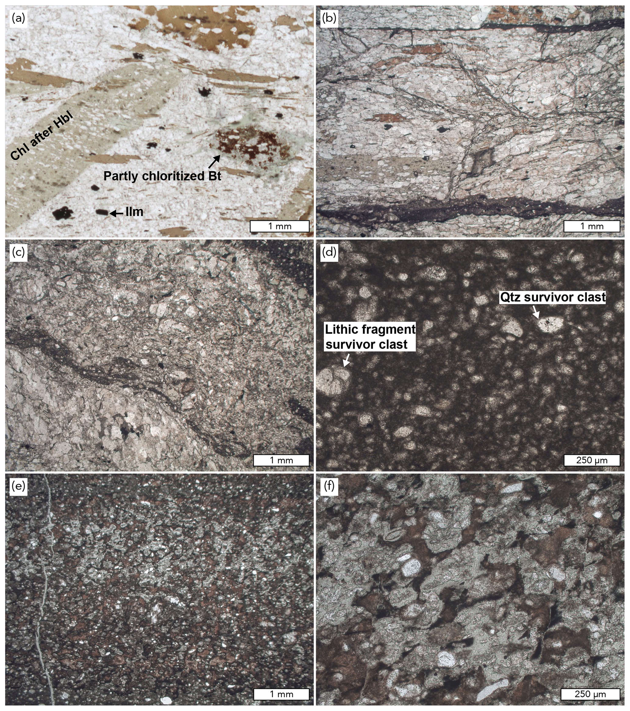
Figure 4Microstructural appearance of host rock and different fault rock types (plane polarized light). (a) Host rock: foliated micaschist with fine-grained (50–200 µm) quartz + white mica + plagioclase matrix and 1 to 10 mm sized porphyroblasts of biotite (fresh: top, partly chloritized: middle right) and pseudomorphs of chlorite after amphibole (left). (b) Brittlely deformed domain in the host rock with multiple fractures filled with cataclasite (center) and/or pseudotachylyte (top and bottom). (c) Cataclastic fault rock: host rock fabric is completely obscured, some lithic fragments remain (bottom left), pseudotachylyte veins occur with patchy and diffuse borders (center, top right corner). (d) Pseudotachylyte: cryptocrystalline matrix containing 20–100 µm sized, spaced survivor clasts of quartz and lithic fragments. (e–f) Spherulitic appearance of altered pseudotachylyte at different scales.
4.1 Host rock microstructure and petrography
Calcareous amphibole–biotite micaschist hosts the fault veins. Large biotite crystals are oriented subparallel to the foliation (Fig. 4a). Some grains show minor replacement by chlorite. Very fine grained (<5 µm), euhedral Ti-oxides occur in the center of patches where chlorite replaced biotite (Fig. 5a). Amphibole is chloritized and only preserved as pseudomorphs (Fig. 4a); their long axes have acute angles () to the foliation plane. The major opaque mineral is ilmenite (Figs. 4a, 5b). Ilmenite breakdown to Ti-oxide is observed at grain boundaries with biotite (Fig. 5b). Boundaries between the brittlely undeformed and fractured host rock or fault or injection veins are sharp (Fig. 4b). In the fractured host rock, alteration of biotite is more pronounced.
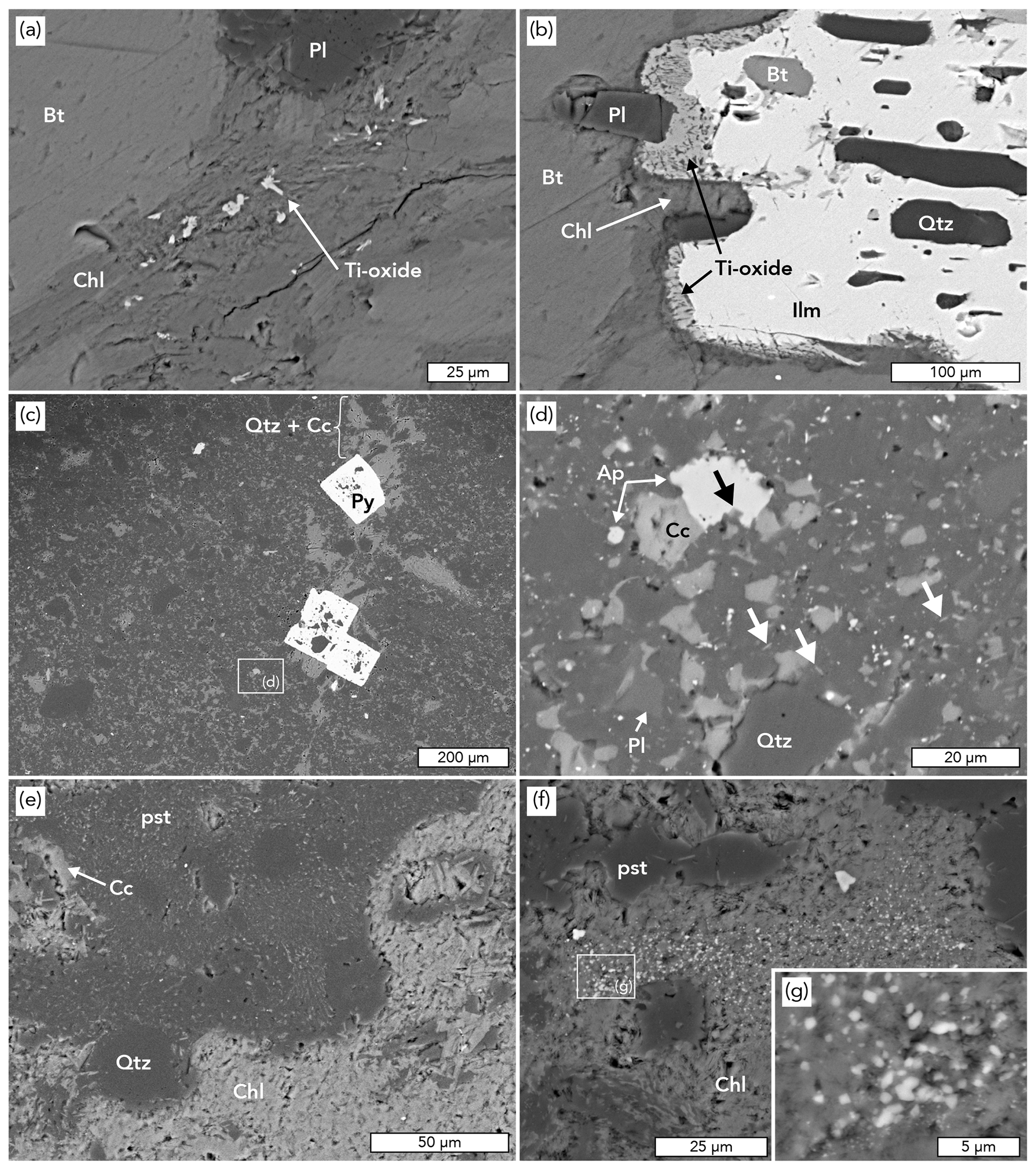
Figure 5Back-scattered electron images of selected microscopic observations. Mineral abbreviations after Whitney and Evans (2010) (a) Breakdown of biotite to chlorite + Ti-oxide + unidentified K-phase. (b) Reaction rim around ilmenite inclusion in biotite: ilmenite + biotite = Ti-oxide + chlorite + unidentified K-phase. (c) Pseudotachylyte with vertical, crosscutting vein with calcite + quartz + pyrite. (d) Microstructure of pseudotachylyte. Calcite (light gray); unknown needle-shaped (white arrows) microcrystallites; and bright, submicrometer-sized oxide/sulfide droplets are dispersed in the cryptocrystalline or amorphous matrix. Note the embayed edges (black arrow) of an apatite survivor clast versus a much smaller, euhedral apatite crystal further left. (e) Meandering alteration front between chloritized and pristine pseudotachylyte. No preferred orientation of chlorite. Note, in contrast, the fan-like growth of microcrystallites in the matrix. (f–g) Micrometer-sized crystals of Ti-oxide (determined by EDS) finely dispersed in chlorite which replaced cryptocrystalline/amorphous pseudotachylyte (pst).
4.2 Fault rock microstructure and petrography
Cataclastic fault rock appears bright in thin section and consists of granular lithic and mineral fragments (Fig. 4c). It forms bulky-to-drawn-out patches that grade into compositional flow banding in fault veins mainly composed of pseudotachylyte (Fig. 3). Within cataclasite patches, tens to hundreds of micrometers thin, curved-to-meandering pseudotachylyte veins occur (Fig. 4c). The modal abundance of cataclasite patches decreases from bottom to top of the studied fault vein (Fig. 3).
Such structural evidence includes microcrystallites, sulfide/oxide droplets and spaced survivor clasts, which may display embayed edges witnessing their melt-assisted corrosion (Magloughlin and Spray, 1992; Kirkpatrick and Rowe, 2013). All of these features are expressed in the studied pseudotachylytes. Sulfide/oxide droplets are submicron in size (Fig. 4d). Grain size of survivor clasts is on the order of 20 to 100 µm (Figs. 4d, 5c, d). Their shapes are generally round, although some exhibit concave, serrated edges (Fig. 5d). Quartz clasts are most common. A smaller amount of subhedral calcite occurs in the fault rock, which most likely represents survivor clasts. Furthermore, <5 µm long needle-shaped crystals without obvious shape-preferred orientation occur dispersed in the cryptocrystalline or amorphous matrix (Fig. 5d). The needle-shaped microcrystallites are probably biotite, as energy-dispersive spectroscopic X-ray (EDS) mapping indicates that they are enriched in Al, K, Fe and Mg compared to the matrix. However, their small size prevented an interpretable single-crystal spectrum. In some places, microcrystallites of unknown composition show dendritic patterns, possibly K-feldspar (sanidine and anorthoclase; Lin, 1994; Fig. 5e).
A 4 to 10 mm wide layer in the upper part of the studied fault vein exhibits a bubbly microstructure in transmitted light (Fig. 4e, f). This spherically meandering microstructure represents chlorite alteration fronts replacing pristine pseudotachylyte (Fig. 5e). The fine-grained (5 to 15 µm) chlorite displays no shape-preferred orientation. Where chlorite has replaced pseudotachylyte, micron- to submicron-sized rhomb-shaped Ti-oxide crystals are finely dispersed (Fig. 5f, g). Their grain size decreases from center to rim of the chloritized domains.
Thin (<0.5 mm) antitaxial calcite + quartz veins with sharp edges cut across the host rock and all types of fault rock. They consist mainly of calcite and subordinate quartz. Euhedral pyrite occurs within such veins or in close proximity (<1 mm, Fig. 3c). Vein orientations generally dip at high angles toward the W or are perpendicular to the foliation. Fibrous calcite, quartz and strain fringes around pyrite are compatible with E–W extension. The veins transect the boundaries between different fault rock types and the host rock without being offset at these boundaries.
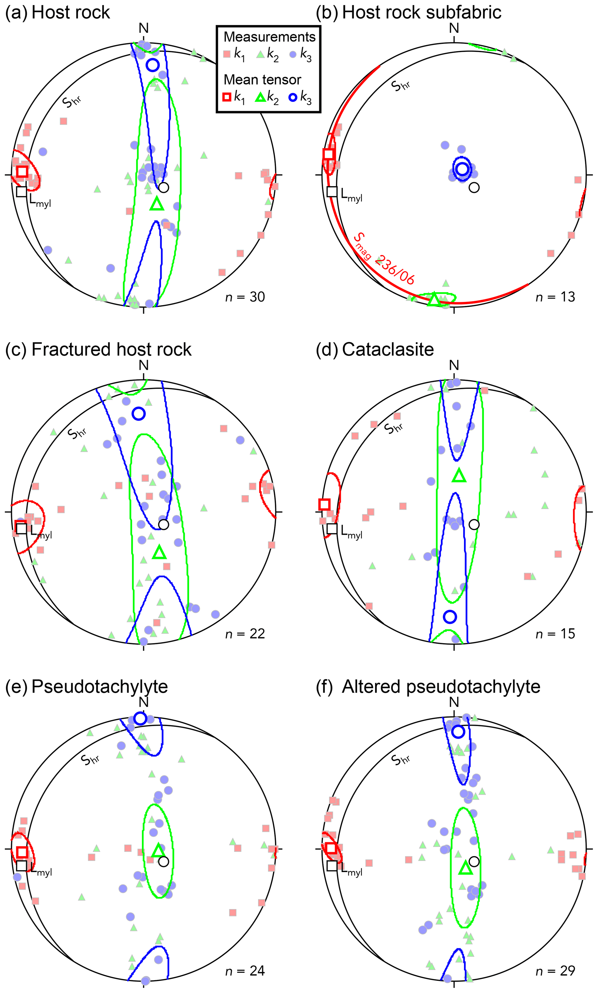
Figure 6(a–f) Lower-hemisphere equal-area projections for principal axes of magnetic anisotropy in different rock types. Comments about data presentation follow: (a) the measurement for specimen AB15-75 was excluded because it was considered an outlier due to its high km (see also Table 1). (e) All data for specimens containing ≥50 % pseudotachylyte were plotted. (f) All data for specimens containing ≥50 % altered pseudotachylyte were plotted.
Table 1Anisotropy of magnetic susceptibility data for host rock and different fault rock types.

5.1 Anisotropy of magnetic susceptibility and frequency-dependent susceptibility
AMS data for all specimens are summarized in Table 1 and graphically presented in Fig. 6. Magnetic anisotropy in host rock and fault rock specimens displays consistent orientations of principal axes. Maximum principal axes (k1) trend E–W and are subparallel to the host rock lineation for all rock types (Fig. 6). Generally, all rock types show prolate AMS symmetry as indicated by distribution of intermediate (k2) and minimum principal axes (k3) in a girdle perpendicular to k1. Furthermore, shapes and orientations of the 95 % confidence regions for mean k2 and k3 axes reflect the prolate AMS shape (Fig. 6a, c–f). Symmetry of these confidence regions indicates that AMS fabrics are similar for the analyzed specimen groups (Borradaile and Jackson, 2010). However, intermediate and minimum principal axes for host rock specimens occur in two clusters (Fig. 6a). One cluster has k3 axes perpendicular to the host rock foliation and k2 axes lying within the foliation plane (Fig. 6b). The corresponding subfabric AMS ellipsoid approaches an oblate shape (). The magnetic foliation expressed by these specimens is subparallel to the schistosity Shr. In the second cluster, k2 and k3 axes are inversely oriented.

Figure 7Variation of anisotropy degree (Pj) and shape (T) parameters for AMS of different rock types. None of the rock types are distinct from the others based on these parameters (a). (b–c) Box-and-whisker plots for Pj and T. HR – host rock, FHR – fractured host rock, CC – cataclasite, PST – pseudotachylyte, APST – altered pseudotachylyte.
Measurements of anisotropy (Pj, T) scatter over similar ranges for all rock types (Fig. 7a). The anisotropy degree Pj shows highest variation for host rock specimens () and lowest for altered pseudotachylyte (). However, the median Pj values are similar in all rock types () and the middle 50 % of these data overlap when shown in box-and-whisker plots (Fig. 7b). The symmetry of the magnetic fabric shows no co-variation with the degree of anisotropy (Fig. 7a). Shapes of AMS ellipsoids for individual specimens of all rock types range from oblate to prolate (Fig. 7c). Overall, neither degree nor shape of the AMS ellipsoid defines a magnetic fabric distinctive for one rock type or a group of several rock types. Nevertheless, the volume-normalized mean susceptibility of altered pseudotachylyte specimens is approximately twice as high (median (SI)) as that of all other rock types (median (SI); Fig. 8).
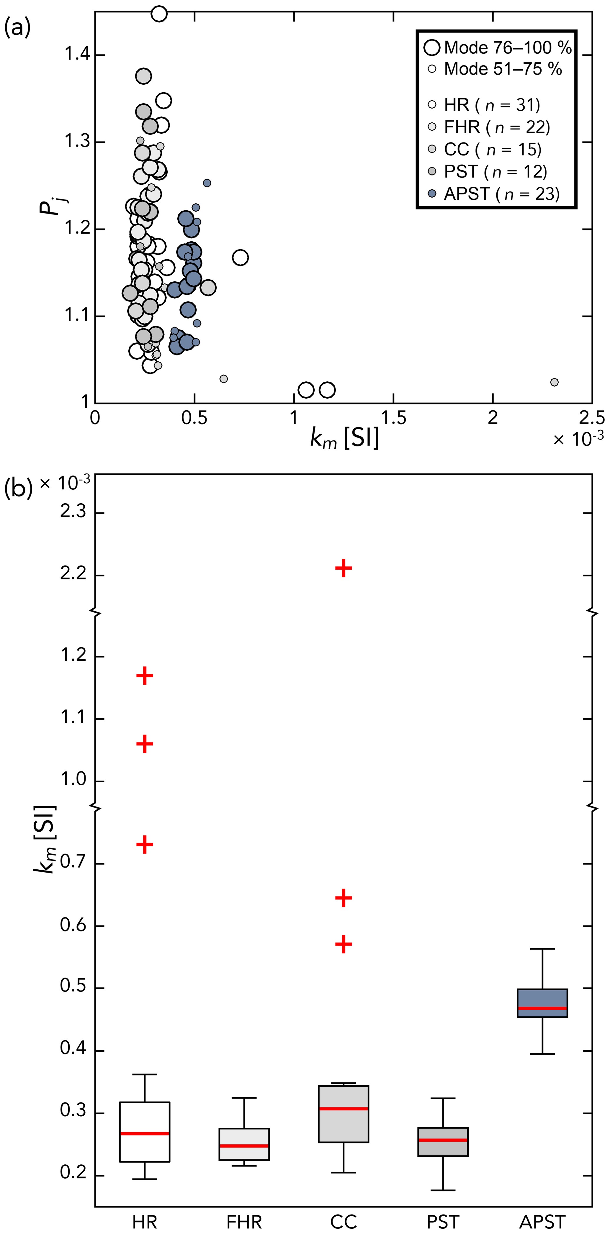
Figure 8(a) Normalized mean susceptibility (kM) versus degree of anisotropy (Pj). The mean susceptibility of altered pseudotachylyte specimens is about twice that of the other rock type specimens (b). For abbreviations, see Fig. 7.
All samples were measured with the three available frequencies used for the MFK1-FA. Figure 9 shows a comparison between mass-dependent susceptibilities measured at frequencies F1 (976 Hz) and F3 (15 616 Hz). Most samples fall along the 1:1 relationship, but it is possible to differentiate samples of pristine pseudotachylyte that have a relatively higher susceptibility compared to other samples (host rock, fractured host rock, cataclasite and altered pseudotachylyte). There is significant scatter in the data, particularly for the pristine pseudotachylytes. The length of the error bars shown in Fig. 9 represents 1 standard deviation based on repeated measurements, with at least three measurements per sample. However, there is a tendency for pristine pseudotachylyte samples to have slightly higher susceptibility at F1 (976 Hz) compared to measurements made at F3 (15 616 Hz).
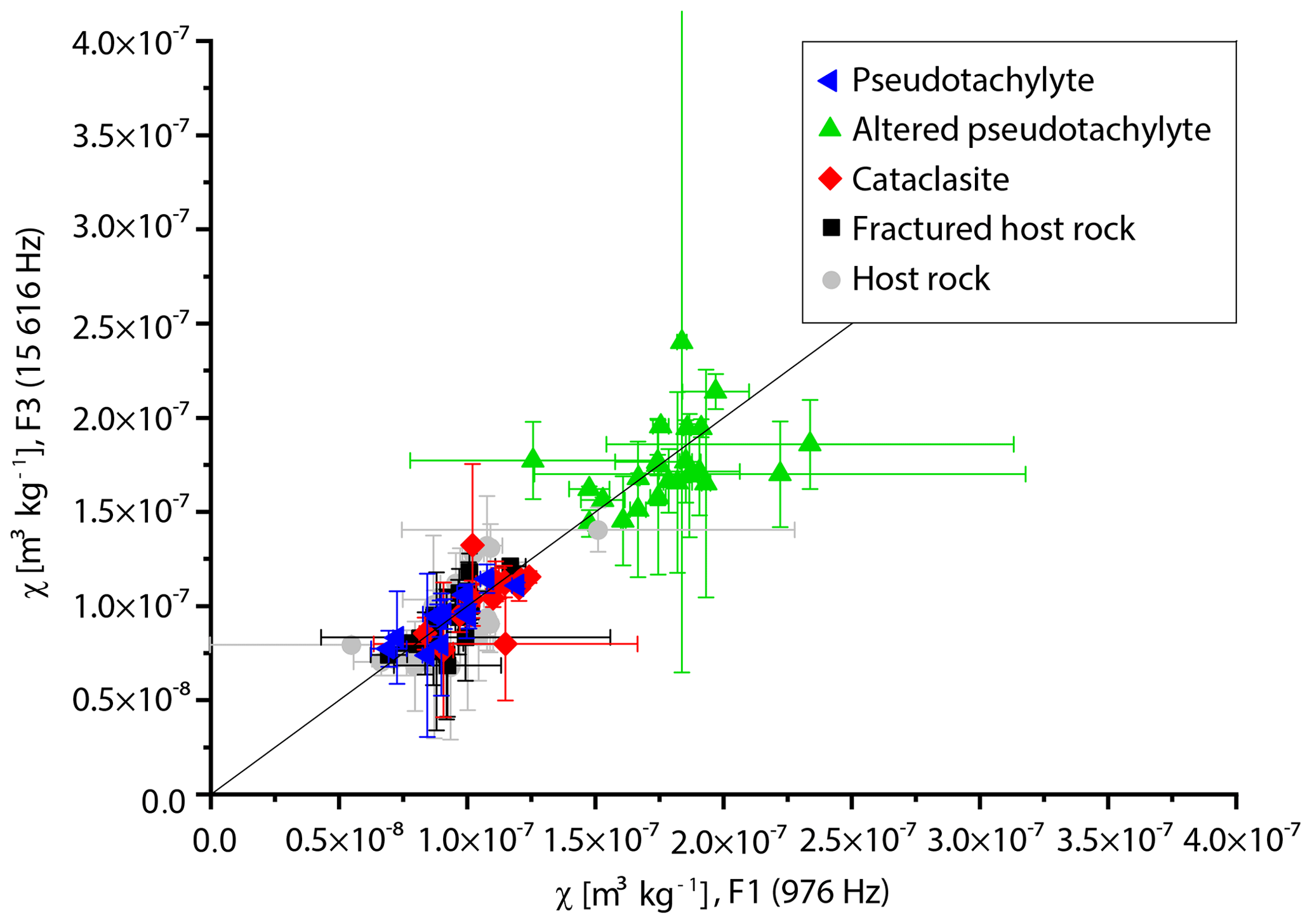
Figure 9Mass-dependent susceptibility (χ) measured as a function of frequency. Error bars represent 1σ standard deviation from repeat measurements of bulk magnetic susceptibility (). Note that the presentation format of data for the different rock types differs compared to Figs. 7 and 8, which present the mean magnetic susceptibility ().
5.2 Temperature dependence of magnetic susceptibility
Thermomagnetic curves for heating and cooling of host rock, as well as for pristine and altered pseudotachylyte, are presented in Fig. 10a–c. With increasing temperature, host rock thermomagnetic data exhibit steadily decreasing magnetic susceptibility, followed first by a rapid increase to about twice the initial value at ca. 500 ∘C and then followed by a rapid decrease at ca. 580 ∘C (specimens AB15-115, AB15-116; Fig. 10d). During cooling, host rock specimens show a prominent rise in susceptibility at temperatures <600 ∘C and a peak at ca. 430 ∘C. Pseudotachylyte specimens (AB15-12, AB15-13∕61, AB15-62) show a small but noticeable drop in susceptibility at 550–590 ∘C (Fig. 10e). During cooling, susceptibility rises sharply for all pseudotachylyte specimens at temperatures <590 ∘C (Fig. 10b). Altered pseudotachylyte exhibits progressively decreasing susceptibility with increasing temperature without any significant drops (specimens AB15-43, AB15-67; Fig. 11f). During cooling, susceptibility progressively increases to a peak at ca. 300 ∘C and then gradually decreases again. For specimen AB15-43, there is a small sharp increase in susceptibility at 590 ∘C observed in the cooling curve.
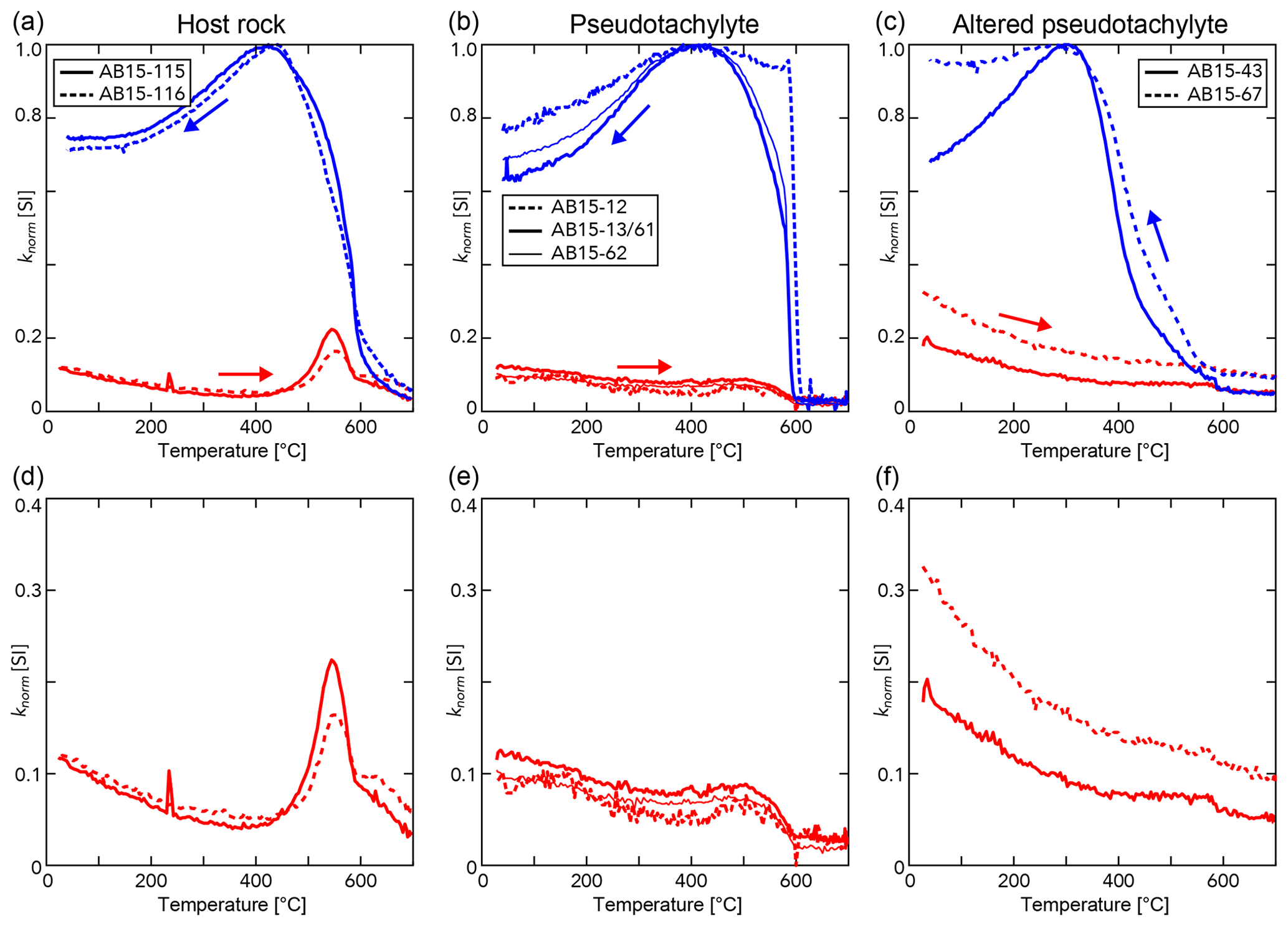
Figure 10(a–c) Thermomagnetic curves for host rock, pristine and altered pseudotachylyte during heating from room temperature to 700 ∘C (red curves) and cooling back to room temperature (blue curves). Susceptibility measurements (knorm) were normalized based on the highest value of each sample during the experiment. For increased visibility of the heating curves, (d)–(f) show only the heating curves for the same specimens shown in (a)–(c).
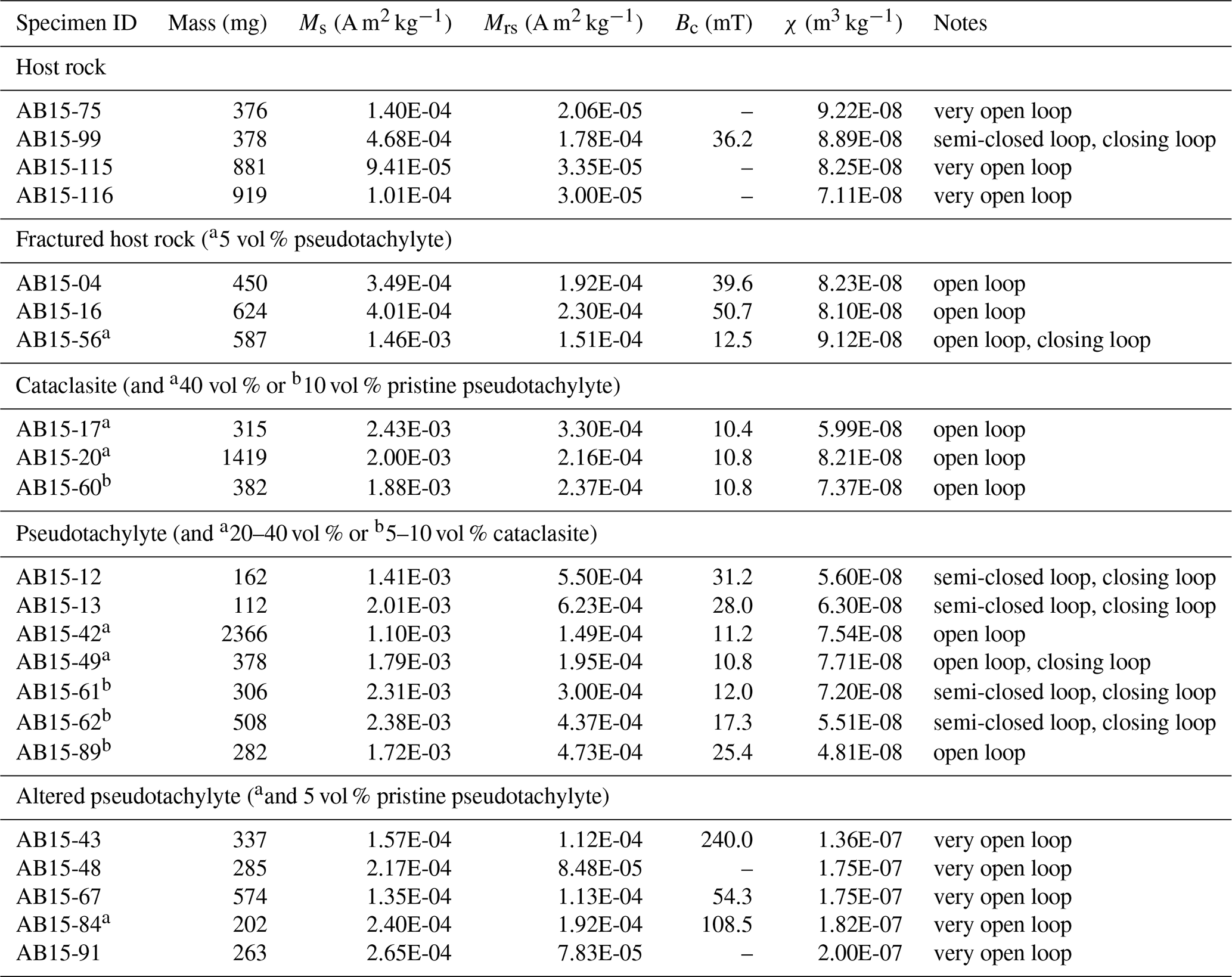
Table 2Magnetic hysteresis parameters for processed hysteresis loops (automatic drift correction and linear high-field slope correction, with a cut-off field of 567 mT). Hysteresis data have been mass normalized. Superscripts a and b in the table refer to relative volume percentages of the different types of fault rock in the samples, as described in Sect. 2.
5.3 Hysteresis loops
Magnetic hysteresis measurements show that all rock types respond dominantly paramagnetically to applied high magnetic fields (Table 2, Fig. 11a, e, i). Hysteresis results for pseudotachylyte-free specimens show either no or very minor ferromagnetic response. They have saturation magnetizations ( A m2 kg−1) about 1 order of magnitude below those specimens containing pseudotachylyte ( A m2 kg−1) (Table 2). Furthermore, pseudotachylyte-free specimens have generally very open slope-corrected hysteresis loops, which do not display branches characteristic of ferromagnetic minerals (Fig. 11b, j) (Paterson et al., 2018). Slope-corrected hysteresis curves for these specimens accordingly also display atypical shapes, which may result from an artificial correction to the data (Fig. 11c, k). Contrastingly, hysteresis loops for pseudotachylyte-bearing specimens show a ferromagnetic contribution in magnetic response. This is expressed weakly in the unprocessed hysteresis loop (Fig. 11e), and more clearly after linear high-field slope correction (Fig. 11f; although hysteresis loops generally fail to close at high fields). Based on hysteresis parameters, pristine pseudotachylyte-rich specimens have the highest saturation remanent magnetization ( A m2 kg−1), compared to host rock ( A m2 kg−1) and altered pseudotachylyte specimens ( A m2 kg−1). Magnetic hysteresis raw data are available in Table S3 in the Supplement.
5.4 Specimen size and shape
Specimen cube dimensions deviate moderately from neutral shapes. Their long edges are between 4.1 % and 20.9 % longer than their short edges. Prolate and oblate shapes are equally common (Fig. 12a, Table S1). The shape parameters of specimen dimensions (Td) and magnetic anisotropy (T) are independent of each other (Fig. 12b, Table S1). The degree of anisotropy of specimen shape and magnetic susceptibility show no significant correlation (Fig. 12c).
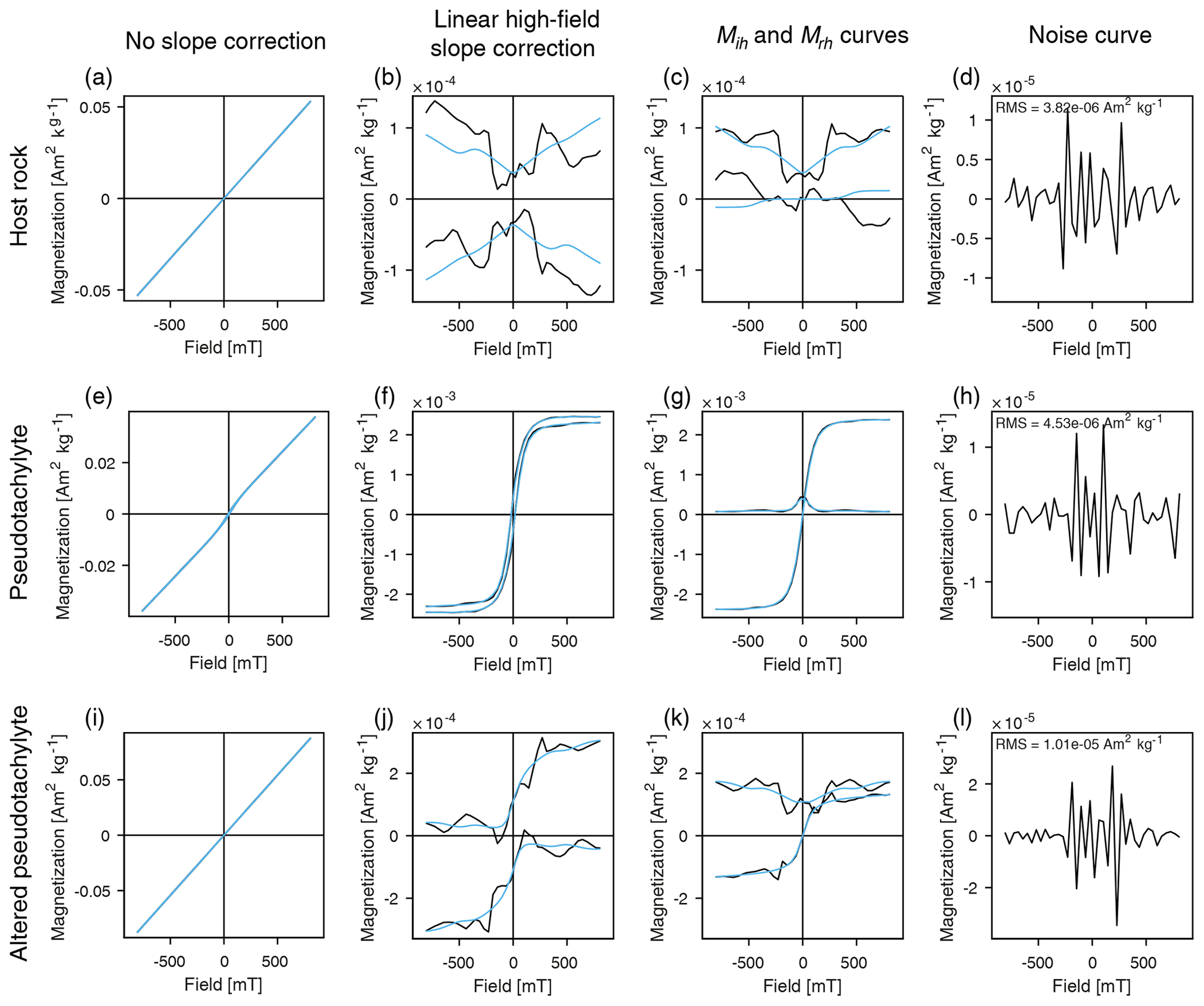
Figure 11Hysteresis results for selected host rock, pseudotachylyte and altered pseudotachylyte specimens. Dominant paramagnetic behaviors of all samples are displayed in raw measurement curves (left column). Panels (a), (e) and (i) show the raw hysteresis loop corrected for the sample mass. Panels (b), (f) and (g) show the hysteresis curve after slope correction. Panels (c), (g) and (k) show the induced hysteresis curve (Mih) and remanence hysteresis curve (Mrh). Panels (d), (h) and (l) show the noise curve of the respective host rock, pseudotachylyte and altered pseudotachylyte, which have been slope corrected for the paramagnetic signal contribution. Processing of hysteresis loops was done with the HystLab software by Paterson et al. (2018).
Raw measurements of mean susceptibility (km) and anisotropy degree (Pj) are inversely proportional (Fig. 13a). The km standard error shows significant correlation with sample volume (Fig. 13b) and degree of anisotropy Pj (Fig. 13c). Additionally, the standard error of km decreases with increasing specimen volume and decreasing mean magnetic susceptibility (Fig. 14). Consequently, the AMS data are dependent on specimen size. Small specimen volumes result in larger uncertainties, which in turn causes higher Pj values. This observation is further discussed in Sect. 6.4 which also discusses the limitation of specimen size in studies using AMS.
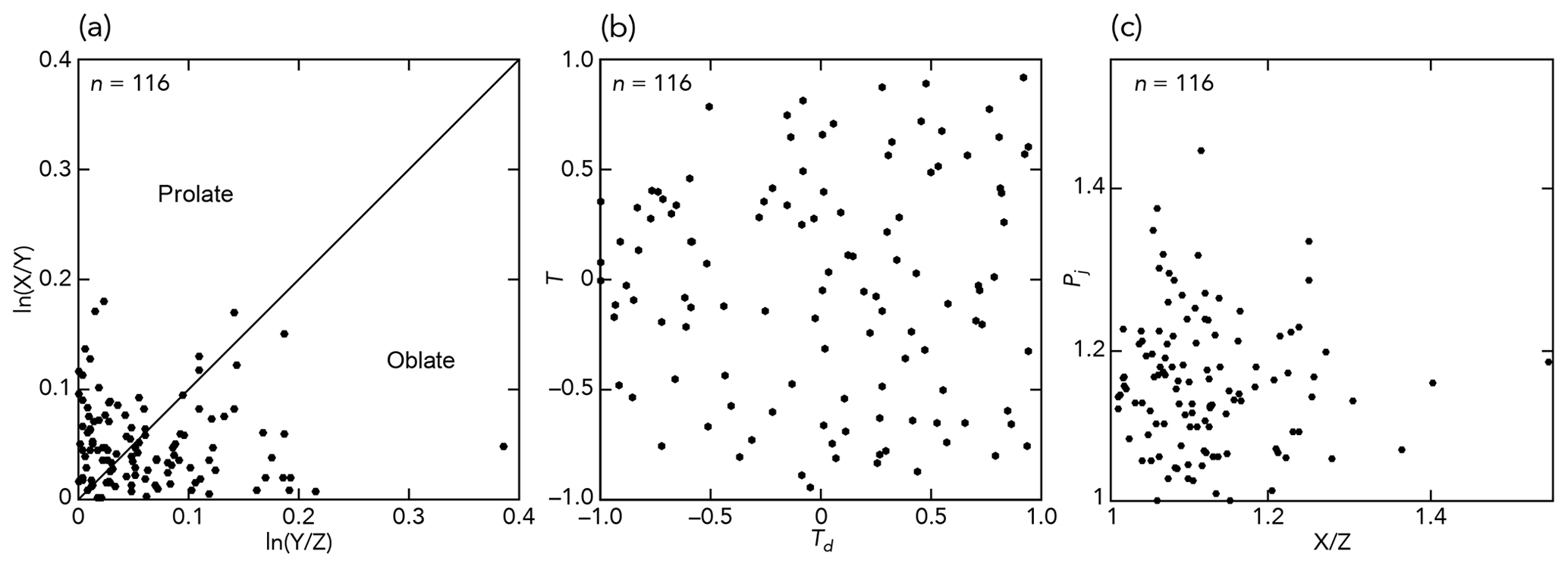
Figure 12Comparison of shape parameters for specimen cubes and AMS ellipsoids. (a) Flinn diagram of specimen dimensions shows that cubes are not perfectly isometric. (b–c) Specimen shape does not seem to exert an influence on either shape or degree of magnetic anisotropy.
6.1 Source of magnetic susceptibility and its anisotropy
Thermomagnetic heating curves for host rock specimens show a decrease in magnetic susceptibility with increasing temperature until 400 ∘C, which is characteristic of paramagnetic behavior (Fig. 10d) (Hunt et al., 1995). Formation of new magnetite at temperatures above 400 ∘C is indicated by the peak and sudden decrease in magnetic susceptibility at 580 ∘C, the Curie temperature of magnetite (Hunt et al., 1995). These results, together with magnetic hysteresis data (Table 2, Fig. 11), show that the magnetic susceptibility of the host rock micaschist arises from paramagnetic minerals. It follows that the AMS in the host rock is controlled by the crystallographic orientation of the paramagnetic minerals (Borradaile and Jackson, 2010). An AMS subfabric in host rock specimens has parallel magnetic and mineral lineations and subparallel magnetic and ductile foliations (Fig. 6b). Shape-preferred orientation of tabular biotite crystals in the host rock (Fig. 4a) implies that crystallographic c axes values of biotite are oriented perpendicular to the schistosity. This AMS subfabric is therefore inferred to originate from crystallographic preferred orientation of biotite, which in single crystals exhibits k3 axes subparallel to biotite crystallographic c axes (Borradaile and Henry, 1997; Martín-Hernández and Hirt, 2003). The mean magnetic susceptibility km of host rock specimens ( (SI)) is in the range of typical of schists ( (SI); Hunt et al., 1995). Single-crystal bulk susceptibility values of biotite, muscovite and chlorite are on the same order of magnitude (around 10−4 (SI)) (Martín-Hernández and Hirt, 2003). In the absence of magnetite, the host rock AMS most likely arises from these sheet silicates. Fractured host rock and cataclasite specimens without pseudotachylyte display the same magnetic properties as host rock specimens (Figs. 7, 8, Tables 1, 2). This conformity suggests the same paramagnetic source of the AMS with contributions from biotite, white mica and chlorite.
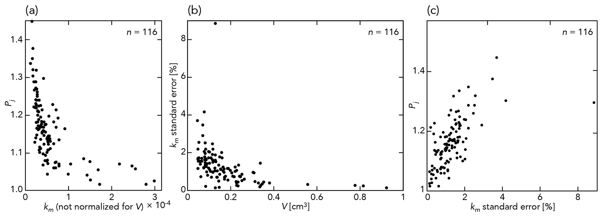
Figure 13Influence of specimen size on the degree of magnetic anisotropy. (a) Without normalization for specimen volume, anisotropy degree (Pj) decreases with increasing mean susceptibility (km). (b) Cube volume plotted against the standard error of the mean susceptibility. (c) Degree of anisotropy (Pj) as a function of standard error (see Sect. 3.2 for the calculation of the standard error).
Pseudotachylyte thermomagnetic data show a distinct drop in susceptibility from 550 to 590 ∘C, which indicates the presence of magnetite (Fig. 10e). Hysteresis results of pseudotachylyte-bearing specimens show mixed paramagnetic and ferromagnetic behaviors (Table 2, Fig. 11e–g). The AMS of pseudotachylytes thus reflects the sum of paramagnetic and ferromagnetic minerals in these specimens. The narrow range of km does not offer the opportunity to isolate subsets (Table 1, Fig. 8), which is a common approach to separate AMS subfabrics caused by paramagnetic and ferromagnetic minerals (Borradaile and Jackson, 2010). The presence of magnetite does not seem to increase km to values significantly higher than the (fractured) host rock and/or cataclasite specimens (Fig. 8). The ferromagnetic contribution to the pseudotachylyte AMS is consequently small. The pseudotachylyte AMS is therefore likely controlled by crystallographic preferred orientation of its paramagnetic minerals, i.e., most probably biotite, with a subordinate contribution from the shape-preferred orientation of magnetite (Sect. 5.2). The nearly absent ferromagnetic response in the slope-corrected hysteresis curves likely means that values of Ms and Mrs are largely artifactual, and samples are dominated by the paramagnetic signal. The exception is pristine pseudotachylyte that does show a weak ferromagnetic behavior after slope correction.
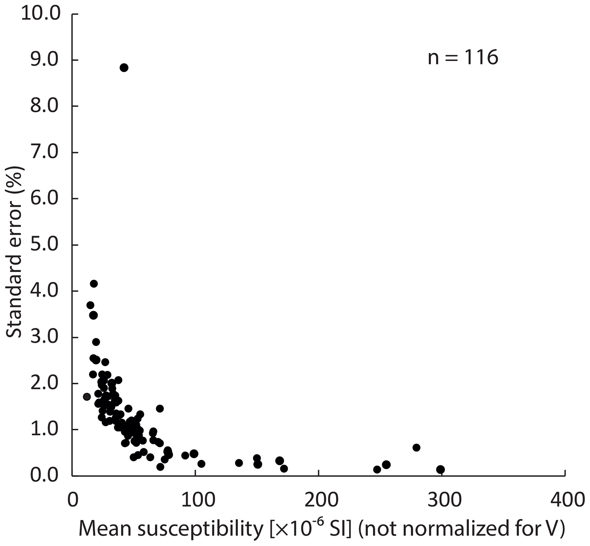
Figure 14Standard error of the mean susceptibility (expressed in %) as a function of mean susceptibility (not normalized for volume).
In altered pseudotachylyte specimens, a successive decrease in magnetic susceptibility without significant drop at 580 ∘C during heating indicates dominant paramagnetic behavior. This behavior suggests that magnetite present in pristine pseudotachylyte has been altered to an unknown phase in chloritized pseudotachylyte (Fig. 10f). Magnetic hysteresis results confirm bulk paramagnetic behavior for altered pseudotachylyte (Table 2, Fig. 11i–k). For the mean magnetic susceptibility for altered pseudotachylyte, being about twice as high as that for other rock types (Table 1, Fig. 8b), the AMS of altered pseudotachylyte apparently has an additional or a different mineral source than the other rock types. Notably, this observation is also made in the high-field susceptibility obtained from hysteresis measurements, which is nearly an order of magnitude higher than in other samples, including the pristine pseudotachylyte (Table 2). Bulk magnetic susceptibility for single-crystal chlorite without high-susceptibility mineral inclusions is about twice that of biotite and muscovite single crystals (Martín-Hernández and Hirt, 2003). These sheet silicates were also argued to collectively cause AMS in host rock specimens, but in altered pseudotachylyte chlorite it is much more abundant, forming up to ca. 50 % of the mode (Figs. 4e, f, 5e–g). We infer that AMS in altered pseudotachylyte dominantly reflects the orientation distribution of chlorite. An alternative explanation for the high susceptibility in the altered pseudotachylytes is the formation of metallic iron during faulting. Zhang et al. (2018) have noted formation of micron-sized iron spherules in pseudotachylytes that were heated within a range of 1300–1500 ∘C, leading to increased magnetic susceptibility. However, no such spherules are directly observed with scanning electron microscopy (Fig. 5), which makes it difficult to evaluate this potential origin for increased susceptibility.
6.2 Petrofabric versus magnetic fabric orientations
The margins of the fault vein are parallel to the slip plane in the Finntjärnen fault zone. Seismic faulting occurred parallel to the schistosity Shr along subhorizontal, shallowly W-dipping shear planes (Figs. 2, 3). The slip direction is indicated by subhorizontal E–W-trending magnetic lineation in all fault rock types (Fig. 6). This direction is consistent with mineral and stretching lineations expressed in the ductilely deformed host rock. These orientations also coincide with the extension direction defined by crosscutting normal faults (Fig. 2b). Obliquity between the pseudotachylyte magnetic foliation and fault vein margins would indicate the kinematics of seismic slip (Ferré et al., 2015). However, the AMS of both cataclastic and friction melt-origin fault rocks displays prolate symmetry and magnetic lineations that are parallel with the vein margins. These results show that neither a magnetic foliation nor obliquity with the shear plane is developed, as would be expected from non-coaxial deformation (Borradaile and Henry, 1997). The observed AMS data raise several questions: (1) If such a kinematic model does not agree with the observed fault rock AMS, what process aligned the maximum principal axes? (2) How is it possible to explain the distribution of intermediate and minimum principal axes in a girdle perpendicular to the k1 axes? (3) Why are AMS fabrics of all rock types compatible? The questions are challenging to answer but they are likely related, given that (1) the magnetic fabrics are coaxial in host rock and pseudotachylytes and (2) the petrofabric and magnetic fabric are coaxial, even though a pronounced magnetic foliation has not developed.
6.3 Deformation sequence and regional tectonic implications
Foliation-parallel fault veins, bound by narrow domains of fractured host rock, crosscut the ductile host rock fabric (Figs. 2–4). Their formation thus postdated ductile upper-greenschist to amphibolite facies deformation, which is in line with previous work (Beckholmen, 1982, 1983, 1984). The fault veins contain unmolten cataclasite, frictional melt-origin pseudotachylyte and altered pseudotachylyte in varying modal amounts. Spaced survivor clasts, microcrystallites and submicron sulfide/oxide droplets in pseudotachylyte identify these fault rocks as quenched, coseismic friction melts (Figs. 4, 5) (Magloughlin and Spray, 1992; Cowan, 1999; Rowe and Griffith, 2015). Chloritization of the pseudotachylyte groundmass and pronounced replacement of biotite by chlorite in fractured host rock domains indicate that hydrothermal alteration was associated with faulting. The chlorite microstructure suggests that recrystallization was static (Fig. 5). After pseudotachylyte formation, ambient temperature conditions in the fault zone are therefore inferred to be of lower greenschist facies (cf. Di Toro and Pennacchioni, 2004; Kirkpatrick et al., 2012). We deduce seismic faulting and subsequent alteration of fault rocks in the Finntjärnen fault zone occurred in the brittle–ductile transition zone near the base of the brittle crust. Assuming a typical temperature range of 300–350 ∘C, depending on the thermal gradient, the faulting occurred at ca. 12±4 km depth (Sibson and Toy, 2006).
Brittle faults and fibrous calcite + quartz veins crosscut both the ductile host rock fabric and the fault veins at high angles. Their orientations relative to the fault vein geometry, together with microscopic and macroscopic observations (Figs. 2–5), suggest that these E–W extensional structures formed latest. These structures are consistent with other extensional structures related to the Røragen Detachment west of the Tännforsen Synform (Fig. 1) (Gee et al., 1994; Bergman and Sjöström, 1997). In summary, seismic faulting in the Finntjärnen fault zone occurred after the formation of the upper greenschist- or amphibolite-facies schistosity and prior to late-stage E–W extensional brittle structures. Structural overprinting relations imply transport of thrust sheets in the Köli Nape Complex during exhumation of these nappes from the middle to the upper crust. The sense of faulting, however, cannot be deduced from the here presented data. Nevertheless, previous work in the area indicated that thrusting was toward the ESE (Bergman and Sjöström, 1997; Bender et al., 2018).
Structural and magnetic analyses of pseudotachylyte-bearing fault veins and their ductilely deformed host rocks reveal that petrofabric and AMS are co-parallel. The accordance of these data indicates that ductile host rock fabrics and brittle fault rock fabrics developed in the same strain field. However, the orientations of AMS and petrofabric in host rock versus fault rock specimens could not be used to deduce the kinematics of ductile or seismic shear. Nevertheless, crosscutting relations show that pseudotachylite formation in the Finntjärnen fault zone predated E–W extensional deformation.
6.4 Methodological remarks on AMS of small specimens
There is an apparent inverse relationship between km and Pj, as well as a linear relationship between degree of anisotropy and standard error of mean susceptibility. This effect appears to be caused by specimen size. The larger specimens (by volume) have in general higher bulk susceptibility, and Pj tends towards lower values ranging from 1.01 up to 1.10. Normalization for specimen volume has little impact on removing this bias, and it is therefore evident that specimens with very small sizes are more likely to produce a large scatter in the degree of anisotropy. Although this seems evident, it is important to remark on. The issue with volume is an undesired artifact and it demonstrates the limitation of using small sample cubes in the current setup with the MFK1-FA system. The effect is furthermore emphasized by the increase in km standard error as a function of Pj.
Observations of magnetic anisotropy made in this study raise the issue of measuring AMS of specimens with small volume. Current equipment that exists commercially is not designed for handling small specimen volumes, and in most applications the intended volume ranges from 7 to 11 cm3 (representing standard size cubes and cylinders used in paleomagnetic and AMS studies). However, there is a growing interest for measurements of small specimens, as many AMS studies target geological structures that occur on the centimeter to sub-centimeter scale (e.g., Ferré et al., 2015). One of the challenges in using smaller specimens is clearly an increased uncertainty in manufacturing specimens that have appropriate dimensions. However, specimens can be constructed with care to compensate for this effect, and in this study we have demonstrated that the non-equidimensional effect is secondary in importance to the specimen volume. Furthermore, our AMS data show a consistent magnetic fabric in the different rock types, which suggests that they most likely represent the true rock fabric, although the magnitudes are variable. It is clear that great care has to be taken when evaluating the anisotropy parameters as a function of sample volume and the bulk susceptibility when small samples are measured. At the same time, there is a desire for further study with smaller samples as this increases the scope of AMS measurements to different geological applications.
Field, microstructural and magnetic fabric data from the Finntjärnen fault zone provide the following constraints on seismic faulting recorded by pseudotachylyte-bearing fault veins:
-
Structural overprinting relations show that seismic faulting occurred during exhumation of the Köli Nappe Complex into the upper crust within the seismic zone and before brittle E–W extension.
-
Neither the petrofabric nor magnetic fabrics reveals the coseismic slip direction, but both host-rock and pseudotachylyte magnetic fabrics indicate dominant E–W subhorizontal to shallowly dipping () transport direction, where the maximum axis of susceptibility is parallel to the structural lineation.
-
Chloritization of pseudotachylyte resulted in higher bulk magnetic susceptibility as compared to pristine pseudotachylyte. The relatively low amount of magnetite in pseudotachylyte is detectable by its magnetic behavior based on thermomagnetic curves, hysteresis loops and bulk susceptibility, but it does not contribute substantially to the pseudotachylyte bulk magnetic behavior.
-
Unconventionally small specimen sizes are promising for detailed and high-resolution measurements of geological features and structures. However, care is needed as the small specimens tend to increase the degree of anisotropy of magnetic susceptibility measurement data, and notably there is a close inverse relationship between specimen volume and standard error of mean susceptibility. Magnetic anisotropy results in small specimens demand cautious interpretation, but they offer a promising new venue to study detailed geological features.
All data that led to the conclusions of this paper are presented in the figures, tables and the Supplement.
The supplement related to this article is available online at: https://doi.org/10.5194/se-11-807-2020-supplement.
Field work was carried out by HB and AB. HB and BSGA conducted the magnetic experiments and processed and interpreted the results. HB and BSGA created figures and tables and wrote the initial draft, which was edited by all co-authors. The revised version of the article was prepared by BSGA.
The authors declare that they have no conflict of interest.
The authors would like to thank Ann Hirt and an anonymous reviewer for valuable comments that helped to significantly improve the article. The authors furthermore thank the editor.
This research has been supported by the Geological Survey of Sweden (grant no. 1760).
The article processing charges for this open-access
publication were covered by Stockholm University.
This paper was edited by Cristiano Collettini and reviewed by Ann Hirt and one anonymous referee.
Beckholmen, M.: Mylonites and pseudotachylites associated with thrusting of the Köli Nappes, Tännforsfältet, Central Swedish Caledonides, Geologiska Föreningen i Stockholm Förhandlingar, 104, 23–32, 1982.
Beckholmen, M.: The deformation sequence in the Häggsjö-Musvalttjärnen-Rensjönäset area in western Jämtland, Swedish Caledonides, Geologiska Föreningen i Stockholm Förhandlingar, 105, 119–130, 1983.
Beckholmen, M.: Structural and Metamorphic Zonation in Tännforsfältet Western Jämtland, Swedish Caledonides, Univ. Stockholm, 82 pp., 1984.
Bender, H., Ring, U., Almqvist, B. S. G., Grasemann, B., and Stephens, M. B.: Metamorphic zonation by out-of-sequence thrusting at back-stepping subduction zones: Sequential accretion of the Caledonian internides, Central Sweden, Tectonics, 37, 3545–3576, https://doi.org/10.1029/2018TC005088, 2018.
Bender, H., Glodny, J., and Ring, U.: Absolute timing of Caledonian orogenic wedge assembly, Central Sweden, constrained by Rb-Sr multi-mineral isochron data, Lithos, 344, 339–359, 2019.
Bergman, A.: The Pseudotachylites of Tännforsfältet,Western Jämtland, Swedish Caledonides, Stockholm University, 75 pp., 2017.
Bergman, S. and Sjöström, H.: Accretion and lateral extension in an orogenic wedge: Evidence from a segment of the Seve-Köli terrane boundary, central Scandinavian Caledonides, J. Struct. Geol., 19, 1073–1091, 1997.
Borradaile, G.: Anisotropy of magnetic susceptibility: rock composition versus strain, Tectonophysics, 138, 327–329, 1987.
Borradaile, G. J. and Henry, B.: Tectonic applications of magnetic susceptibility and its anisotropy, Earth Sci. Rev., 42, 49–93, 1997.
Borradaile, G. J. and Jackson, M.: Structural geology, petrofabrics and magnetic fabrics (AMS, AARM, AIRM), J. Struct. Geol., 32, 1519–1551, https://doi.org/10.1016/j.jsg.2009.09.006, 2010.
Butler, R. F.: Paleomagnetism: Magnetic domains to geologic terranes, Electron. Ed., 238 pp., 1998.
Cañón-Tapia, E. and Castro, J.: AMS measurements on obsidian from the Inyo Domes, CA: A comparison of magnetic and mineral preferred orientation fabrics, J. Volcanol. Geotherm. Res., 134, 169–182, 2004.
Cowan, D. S.: Do faults preserve a record of seismic slip?, A field geologist's opinion, J. Struct. Geol., 21, 995–1001, 1999.
Dearing, J. A., Dann, R. J. L., Hay, K., Lees, J. A., Loveland, P. J., Maher, B. A., and O'Grady, K.: Frequency-dependent susceptibility measurements of environmental materials, Geophys. J. Int., 124, 228–240, 1996.
Di Toro, G. and Pennacchioni, G.: Superheated friction-inducde melts in zoned pseudotachylytes within the Adamello tonalites (Italian Southern Alps), J. Struct. Geol., 26, 1783–1801, 2004.
Di Toro, G., Nielsen, S., and Pennacchioni, G.: Earthquake rupture dynamics frozen in exhumed ancient faults, Nature, 436, 1009–1012, https://doi.org/10.1038/nature03910, 2005.
Ernst, R. E. and Baragar, W. R. A.: Evidence from magnetic fabric for the flow pattern of magma in the Mackenzie giant radiating dyke swarm, Nature, 356, 511–513, 1992.
Ferré, E. C., Geissman, J. W., and Zechmeister, M. S.: Magnetic properties of fault pseudotachylytes in granites, J. Geophys. Res.-Sol. Ea., 117, 1–25, https://doi.org/10.1029/2011JB008762, 2012.
Ferré, E. C., Geissman, J. W., Demory, F., Gattacceca, J., Zechmeister, M. S., and Hill, M. J.: Coseismic magnetization of fault pseudotachylytes: 1. Thermal demagnetization experiments, J. Geophys. Res.-Sol. Ea., 119, 6113–6135, 2014.
Ferré, E. C., Geissman, J. W., Chauvet, A., Vauchez, A., and Zechmeister, M. S.: Focal mechanism of prehistoric earthquakes deduced from pseudotachylyte fabric, Geology, 43, 531–534, https://doi.org/10.1130/G36587.1, 2015.
Fossen, H.: Structural Geology, Cambridge University Press, Cambridge, 463 pp., 2010.
Fukuchi, T.: Strong ferrimagnetic resonance signal and magnetic susceptibility of the Nojima pseudotachylyte in Japan and their implication for coseismic electromagnetic changes, J. Geophys. Res.-Sol. Ea., 108, 1–8, https://doi.org/10.1029/2002JB002007, 2003.
Gee, D. G., Lobkowicz, M., and Singh, S.: Late Caledonian extension in the scandinavian Caledonides-the Røragen Detachment revisited, Tectonophysics, 231, 139–143, https://doi.org/10.1016/0040-1951(94)90126-0, 1994.
Hirt, A. M. and Almqvist, B. S. G.: Unraveling magnetic fabrics, Int. J. Earth Sci., 101, 613–624, https://doi.org/10.1007/s00531-011-0664-0, 2012.
Hrouda, F.: Models of frequency-dependent susceptibility of rocks and soils revisited and broadened, Geophys. J. Int., 187, 1259–1269, 2011.
Hunt, C. P., Moskowitz, B. M., and Banarjee, S. K.: Magnetic properties of rocks and minerals, Rock Physics and Phase Relations, A Handbook of Physical Constants, AGU Reference Shelf, 3, 189–204, 1995.
Jelinek, V.: Characterization of the magnetic fabric of rocks, Tectonophysics, 79, 63–67, 1981.
Jelínek, V.: Measuring anisotropy of magnetic susceptibility on a slowly spinning specimen – basic theory, AGICO Print No. 10. (leaflet), 27 pp., 1996.
Kirkpatrick, J. D. and Rowe, C. D.: Disappearing ink: How pseudotachylytes are lost from the rock record, J. Struct. Geol., 52, 183–198, 2013.
Kirkpatrick, J. D., Dobson, K. J., Mark, D. F., Shipton, Z. K., Brodsky, E. E., and Stuart, F. M.: The depth of pseudotachylyte formation from detailed thermochronology and constraints on coseismic stress drop variability, J. Geophys. Res., 117, B06406, doi:10.1029/2011JB008846, 2012.
Lin, A.: Microlite morphology and chemistry in pseudotachylite, from the Fuyun Fault Zona, China, J. Geol., 102, 317–329, 1994.
Lin, A.: Fossil Earthquakes: The Formation and Preservation of Pseudotachylytes, Spinger, 348 pp., 2008.
Magloughlin, J. F. and Spray, J. G.: Frictional melting processes and products in geological materials: introduction and discussion, Tectonophysics, 204, 197–204, 1992.
Marrett, R. and Allmendinger, R. W.: Kinematic analysis of fault-slip data, J. Struct. Geol., 12, 973–986, https://doi.org/10.1016/0191-8141(90)90093-E, 1990.
Martín-Hernández, F. and Hirt, A. M.: The anisotropy of magnetic susceptibility in biotite, muscovite and chlorite single crystals, Tectonophysics, 367, 13–28, 2003.
Nakamura, N., Hirose, T., and Borradaile, G. J.: Laboratory verification of submicron magnetite production in pseudotachylytes: Relevance for paleointensity studies, Earth Planet. Sci. Lett., 201, 13–18, https://doi.org/10.1016/S0012-821X(02)00704-5, 2002.
Paterson, G. A., Zhao, X., Jackson, M., and Heslop, D.: Measuring, processing, and analyzing hysteresis data, Geochem. Geophy. Geosy., 19, 1925–1945, 2018.
Rowe, C. D. and Griffith, W. A.: Do faults preserve a record of seismic slip: A second opinion, J. Struct. Geol., 78, 1–26, https://doi.org/10.1016/j.jsg.2015.06.006, 2015.
Scott, R. G. and Spray, J. G.: Magnetic fabric constraints on friction melt flow regimes and ore emplacement direction within the South Range Breccia Belt, Sudbury Impact Structure, Tectonophysics, 307, 163–189, https://doi.org/10.1016/S0040-1951(99)00124-9, 1999.
Sibson, R. H.: Generation of pseudotachylyte by ancient seismic faulting, Geophys. J. Int., 43, 775–794, 1975.
Sibson, R. and Toy, V.: The Habitat of Fault-Generated Pseudotachylyte: Presence vs. Absence of Friction-Melt, in: Earthquakes: Radiated Energy and the Physics of Faulting, Geophysical Monograph Series 170, American Geophysical Union, doi:10.1029/170GM16, 2006.
Tarling, D. and Hrouda, F.: Magnetic anisotropy of rocks, Springer Science & Business Media, 217 pp., 1993.
Tauxe, L.: Essentials of paleomagnetism, First Edit., University of California Press, Berkeley, Los Angeles, London, 489 pp., 2010.
Zhang, L., Haibing, L., Sun, Z., Chou, Y.-M., Cao, Y., and Wang, H.: Metallic iron formed by melting: A new mechanism for magnetic highs in pseudotachylyte, Geology, 46, 779–782, 2018.
- Abstract
- Introduction
- Regional geological context and field and macroscopic appearance of fault veins
- Sampling, materials and analytical techniques
- Microstructural description of host and fault rocks
- Rock magnetism results
- Discussion
- Conclusions
- Data availability
- Author contributions
- Competing interests
- Acknowledgements
- Financial support
- Review statement
- References