The hydraulic efficiency of single fractures: correcting the cubic law parameterization for self-affine surface roughness and fracture closure

Quantifying the hydraulic properties of single fractures is a fundamental requirement to understand fluid flow in fractured reservoirs. For an ideal planar fracture, the effective flow is proportional to the cube of the fracture aperture. In contrast, real fractures are rarely planar, and correcting the cubic law in terms of fracture roughness has therefore been a subject of numerous studies in the past. Several empirical relationships between hydraulic and mechanical aperture have been proposed based on statistical variations of the aperture field. However, often, they exhibit non-unique solutions, attributed to the geometrical variety of naturally occurring fractures.

In this study, a non-dimensional fracture roughness quantification scheme is acquired, opposing effective surface area against relative fracture closure. This is used to capture deviations from the cubic law as a function of quantified fracture roughness, here termed hydraulic efficiencies. For that, we combine existing methods to generate synthetic 3-D fracture voxel models. Each fracture consists of two random, 25 cm² wide self-affine surfaces with prescribed roughness amplitude, scaling exponent, and correlation length, which are separated by varying distances to form fracture configurations that are broadly spread in the newly formed two-parameter space (mean apertures in submillimeter range).

First, we performed a percolation analysis on 600 000 synthetic fractures to narrow down the parameter space on which to conduct fluid flow simulations. This revealed that the fractional amount of contact and the percolation probability solely depend on the relative fracture closure.

Next, Stokes flow calculations are performed, using a 3-D finite differences code on 6400 fracture models to compute directional permeabilities. The deviations from the cubic law prediction and their statistical variability for equal roughness configurations were quantified. The resulting 2-D solution fields reveal decreasing cubic law accordance down to 1 % for extreme roughness configurations. We show that the non-uniqueness of the results significantly reduces if the correlation length of the aperture field is much smaller than the spatial extent of the fracture. An equation was provided that predicts the average behavior of hydraulic efficiencies and respective fracture permeabilities as a function of their statistical properties. A model to capture fluctuations around that average behavior with respect to their correlation lengths has been proposed. Numerical inaccuracies were quantified with a resolution test, revealing an error of 7 %.

By this, we propose a revised parameterization for the permeability of rough single fractures, which takes numerical inaccuracies of the flow calculations into account. We show that this approach is more accurate compared to existing formulations. It can be employed to estimate the permeability of fractures if a measure of fracture roughness is available, and it can readily be incorporated in discrete fracture network modeling approaches.

1 Introduction

The geometrical inhomogeneities of single fractures and their effect on fluid flow remain a crucial parameter for understanding the hydraulic properties of fractured reservoirs, such as crystalline or tight carbonate rocks with nearly impermeable matrices. Hence, it has wide-ranging industrial applicability in the fields of petroleum and gas production, geothermal energy recovery, CO₂ sequestration, nuclear waste disposal, and groundwater management. Fluid flow in fractured reservoirs is commonly modeled by the discrete-fracture-network (DFN) approach (Bogdanov et al., 2003; Klimczak et al., 2010; Leung et al., 2012; de Dreuzy et al., 2012), which relies on knowing the permeability of single fractures. The permeability of a single fracture is often approximated by the well-known cubic law (Snow, 1969; Witherspoon et al., 1980), assuming that a fracture is composed of two parallel plates separated by a constant aperture. However, natural fracture walls show deviations from planarity, i.e., roughness, resulting in varying apertures within the fracture plane. On top of that, fluid–rock interactions like dissolution (Durham et al., 2001), erosion (Pyrak-Nolte and Nolte, 2016), and mineral growth (Kling et al., 2017), as well as the surrounding stress field (Zimmerman and Main, 2004; Azizmohammadi and Matthäi, 2017) further modify the geometry of a fracture, causing deviations of the parallel plate assumption.

Considerable effort has been made to study the effect of fracture surface roughness on flow and reactive transport behavior. Early attempts (Patir and Cheng, 1978; Brown, 1987; Zimmerman and Bodvarsson, 1996; Oron and Berkowitz, 1998) employed the 2-D Reynolds equation, a simplification of the Navier–Stokes equations, which assumes that the cubic law holds locally with the aperture varying in the x–y along-fracture plane. They derived semi-empirical functions that describe the deviations from the cubic law in terms of the mean and standard deviation of the aperture field. Increasing computational power led to numerical improvements, with 3-D lattice Boltzmann (Jin et al., 2017; Foroughi et al., 2018) or Navier–Stokes (Mourzenko et al., 1995; Brush and Thomson, 2003) simulations revealing the non-uniqueness of previous functional approximations of fracture permeability. Factors such as shear displacement (Kluge et al., 2017), tortuosity, and the degree of mismatch between the opposing fracture surfaces (Mourzenko et al., 2018) were demonstrated to affect fluid flow paths and permeabilities. Detailed analyses of exposed fracture surfaces have shown that self-affine fractal models are capable of quantifying surface roughness properties from thin section scale to outcrop scale. Thereby, the dependence of surface roughness as a function of observation scale is captured by their scaling exponent (the so-called Hurst exponent, H). For example, mode I fractures in a porous sandstone showed H of 0.4–0.5 (Boffa et al., 1998; Ponson et al., 2007). Microfractures in Pomeranian shale featured H of 0.3 and 0.5 (Pluymakers et al., 2017), depending on the opening mode. In other studies, H of fault surfaces (mode II fractures) tends to fall in the range of 0.6–0.8 with respect to slip orientation (Power and Tullis, 1991; Schmittbuhl et al., 1995; Bouchaud, 1997; Renard et al., 2006; Candela et al., 2012), regardless of rock type. Based on this, it is commonly assumed that a fracture consists of two opposing self-affine surfaces, and the resulting aperture field follows the same scaling relationship, assuming both surfaces are uncorrelated (Plouraboué et al., 1995). However, observations of opposing fracture walls (Brown, 1995) have demonstrated that the two surfaces tend to be well correlated above a specific length scale and non-correlated below it, which poses an upper limit to the self-affine scaling in nature. Following Méheust and Schmittbuhl (2001, 2003), the ratio between system size (L) and the correlation length (l_c) defines whether the fracture has an intrinsic permeability or not. Their statistical approach suggested that permeabilities of uncorrelated fractures (i.e., $l_{\mathrm{c}}/L=\mathrm{1}$) are strongly fluctuating and anisotropic for the same roughness configurations, revealing the importance of considering low l_c∕L ratios to be able to quantify an intrinsic fracture permeability.

Although extensively studied, no clear mathematical relationship between fracture roughness and permeability has been derived so far, leaving the cubic law as standardized parameterization in DFN modeling approaches. Thus, an applicable refinement is desired to promote their realism to help better understanding fluid flow on a reservoir scale. In this paper, existing algorithms are used to generate a large dataset of synthetic fractures covering all possible kinds of roughness configurations. Single-phase 3-D Stokes flow calculations are then performed with a finite difference code, utilizing a high-performance-computing (HPC) cluster to handle the associated computational effort. By interpreting the statistical variations of the results, a refined parameterization of single-fracture permeability is proposed, which is demonstrated to provide accurate predictions for the permeability of rough fractures.

2 Method and data

2.1 Fluid flow in self-affine fractures

Generally, the flow of an incompressible Newtonian fluid is most accurately described by the Navier–Stokes equations (NSEs). Assuming that the flow is solely laminar (Reynolds numbers below unity according to Zimmerman and Bodvarsson, 1996), the fluid viscosity is constant, and gravity is negligible at the system size, they reduce to the simpler Stokes equations, i.e., momentum balance (Eq. 1) and continuity (Eq. 2) equations, which for steady-state flow conditions are given in compact form by

$$\begin{array}{}\text{(1)}& {\displaystyle }\mathit{\mu }{\mathrm{\nabla }}^{\mathrm{2}}\mathit{v}=\mathrm{\nabla }P,\text{(2)}& {\displaystyle }\mathrm{\nabla }\cdot \mathit{v}=\mathrm{0},\end{array}$$

with the fluid's dynamic viscosity μ, pressure P, and velocity vector $\mathit{v}=(v_x,v_y,v_z)$, ∇, ∇⋅, and ∇² denote the gradient, divergence, and Laplace operator for 3-D Cartesian coordinates, respectively.

These equations can be solved analytically for an idealized fracture, consisting of two parallel plates, vertically separated by a constant aperture a. Volumetric integration of the horizontally extended Poiseuille-flow solution yields the well-known cubic law:

$$\begin{array}{}\text{(3)}& Q=-{\displaystyle \frac{w{a}^{\mathrm{3}}\mathrm{\Delta }P}{\mathrm{12}\mathit{\mu }}},\end{array}$$

with total volumetric flow rate Q, fracture width w, and pressure gradient along the fracture ΔP (see Zimmerman and Bodvarsson, 1996 for a more detailed derivation). Combining Eq. (3) with Darcy's law for flow through porous media,

$$\begin{array}{}\text{(4)}& Q=-{\displaystyle \frac{kA\mathrm{\Delta }P}{\mathit{\mu }}},\end{array}$$

with cross-sectional area A, leaves the intrinsic permeability k of an idealized fracture proportional to its aperture by $k\propto a^{\mathrm{2}}/\mathrm{12}$. For a rough walled fracture, the aperture is no longer constant but rather varying across the fracture plane. The mean planes of an upper and lower rough surface s_u(x,y) and s_l(x,y) are separated by a constant distance d to form a(x,y) according to

$$\begin{array}{}\text{(5)}& a(x,y)=\left[s_{\mathrm{u}}(x,y)+{\displaystyle \frac{d}{\mathrm{2}}}\right]-\left[s_{\mathrm{l}}(x,y)-{\displaystyle \frac{d}{\mathrm{2}}}\right].\end{array}$$

Depending on d, the surfaces may overlap at certain points and form contact areas, such that a₀(x,y) is zero at these locations:

$$\begin{array}{}\text{(6)}& a_{\mathrm{0}}(x,y)=\left\{\begin{array}{ll}a& \text{if }a(x,y)>\mathrm{0}\\ \mathrm{0}& \text{if }a(x,y)\le \mathrm{0}.\end{array}\right.\end{array}$$

Assuming that s_u and s_l are self-affine, the standard deviation σ of the aperture field computed at system size l scales as (Brown, 1995; Schmittbuhl et al., 1995):

$$\begin{array}{}\text{(7)}& \mathit{\sigma }=\left\{\begin{array}{ll}\mathit{\beta }{l}^H& \text{if }\mathrm{0}\le l\le l_{\mathrm{c}}\\ \mathit{\beta }{l}_{\mathrm{c}}^H& \text{if }{l}_{\mathrm{c}}\le l\le L,\end{array}\right.\end{array}$$

with the maximal system size L and the correlation length l_c. Below l_c, the fracture is uncorrelated, and it is well correlated above it (see Fig. 1 for a visual explanation). The prefactor β delivers information about the overall amplitude of the surface roughness. H typically denotes the scaling or Hurst exponent with $\mathrm{0}<H\le \mathrm{1}$, whereas H=1 corresponds to self-similar and H<1 to self-affine scaling (e.g., Mandelbrot, 1983). Physically, self-affinity is expressed by higher height fluctuations at smaller scales, leaving H as a measure for the ratio of large-scale versus small-scale roughness intensity.

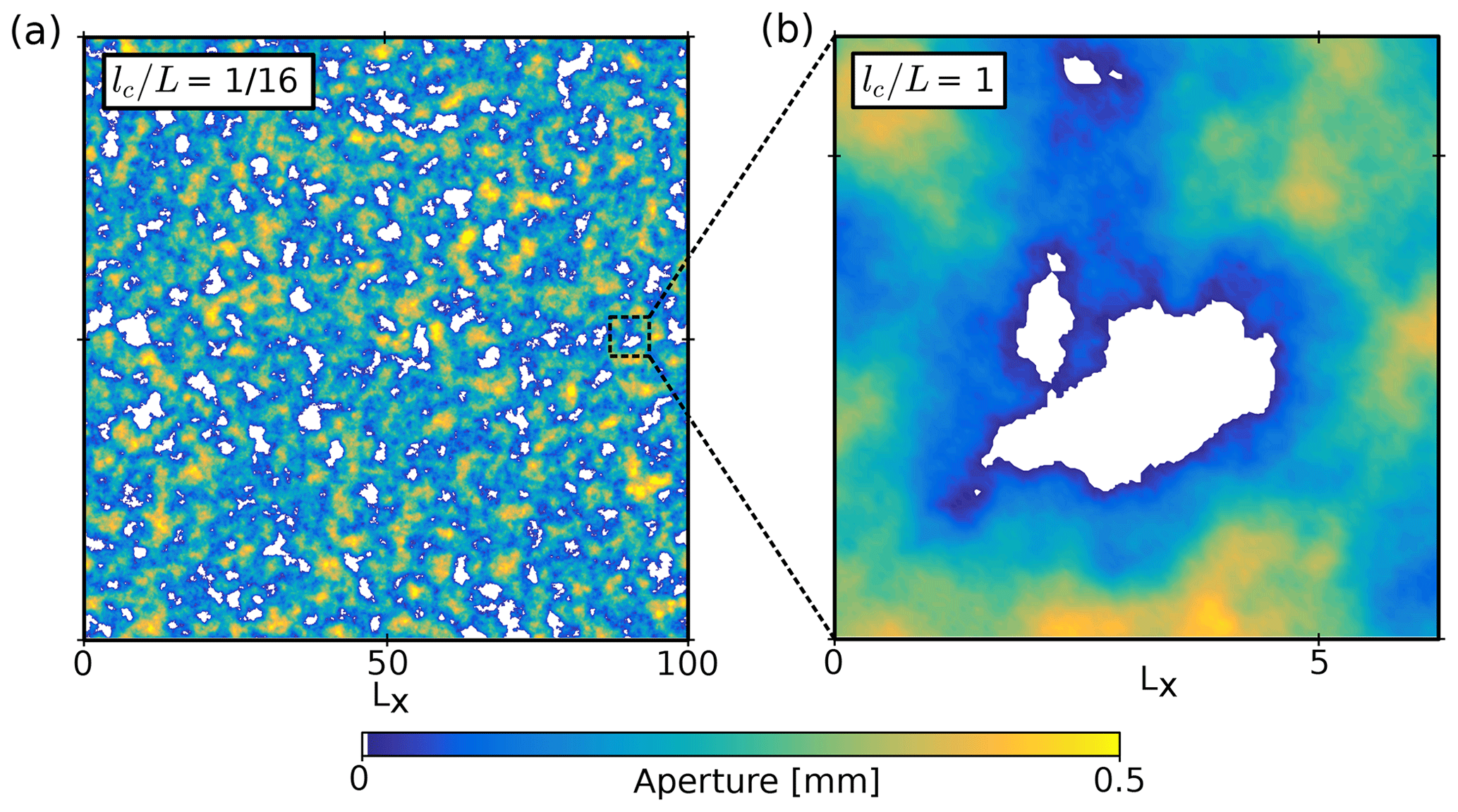
Figure 1 (a) Aperture field of a synthetically generated fracture (d=1 mm, σ_s=0.5 mm, H=0.9) with a l_c∕L ratio of 1∕16. (b) Zoomed-in image showing the uncorrelated part of the aperture field. Units of L_x are in millimeters.

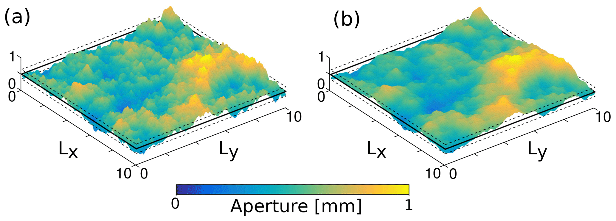
Figure 2 Two aperture fields constructed from synthetic fractures. Both aperture fields are based on the same sets of random numbers with varying Hurst exponents H, which are (a) 0.4 and (b) 0.8. The two statistical parameters ($\stackrel{\mathrm{‾}}{a}$ and σ_a) are indicated by solid and dashed black lines, respectively. Axis units are in millimeters, while the vertical axis (indicating aperture) is exaggerated by a factor of 2 for clarity. Note that $\stackrel{\mathrm{‾}}{a}$ and σ_a are identical for panels (a) and (b). Increasing height fluctuations at smaller scales, caused by a lower Hurst exponent, results in a larger effective surface area S for fracture (a) compared to panel (b).

Here, we use the following two non-dimensional quantities to quantify the geometry of a rough fracture: (i) the relative closure R and (ii) the effective surface area S. We compute the relative closure by dividing the standard deviation of the aperture field at the maximal system size σ_a by the average aperture field $\stackrel{\mathrm{‾}}{a}$:

$$\begin{array}{}\text{(8)}& R={\displaystyle \frac{{\mathit{\sigma }}_{\mathrm{a}}}{\stackrel{\mathrm{‾}}{a}}},\end{array}$$

with $\stackrel{\mathrm{‾}}{a}$ defined by

$$\begin{array}{}\text{(9)}& \stackrel{\mathrm{‾}}{a}={\displaystyle \frac{\mathrm{1}}{L_x{L}_y}}\underset{x=\mathrm{0}}{\overset{L_x}{\int }}\underset{y=\mathrm{0}}{\overset{L_y}{\int }}{a}_{\mathrm{0}}(x,y)\mathrm{d}x\mathrm{d}y.\end{array}$$

This quantity or its reciprocal is commonly used to infer the amount of contact between the opposing fracture walls (Patir and Cheng, 1978; Brown, 1987; Zimmerman and Bodvarsson, 1996; Méheust and Schmittbuhl, 2000). Theoretically, it falls in the range $\mathrm{0}<R\le \mathrm{\infty }$, whereas R=0 shows perfect accordance with parallel plates and the surfaces are in contact if $R\ge (\mathrm{3}\sqrt{\mathrm{2}}{)}^{-\mathrm{1}}$ (see Brown, 1987).

Furthermore, one requires a parameter that quantifies the effective surface roughness of a fracture since fractures with different H can have equal R values (see Fig. 2 for a visualization of the non-uniqueness of R). We therefore introduce a new quantity, the “effective surface area S”. This parameter uniquely combines varying amplitudes and scaling exponents, because an increase in fracture surface area is the direct consequence of increasing roughness. For that, we calculate the ratio of the surface area of the fracture sa_f to twice the area of its projection on the fracture plane (i.e., 2 times the base area perpendicular to the flow direction) sa_c and normalize it with the fractional amount of the aperture field that has opened, i.e.,

$$\begin{array}{}\text{(10)}& S=\left({\displaystyle \frac{{\mathrm{sa}}_{\mathrm{f}}}{{\mathrm{sa}}_{\mathrm{c}}}}\right)\left({\displaystyle \frac{\mathrm{1}}{\mathrm{1}-c}}\right),\end{array}$$

with c being the contact fraction of the aperture field (i.e., where $a_{\mathrm{0}}(x,y)=\mathrm{0}$), which leaves $\mathrm{1}\le S\le \mathrm{\infty }$, with S=1, showing perfect accordance with parallel plates. To finally quantify the influence of fracture roughness on its intrinsic permeability, the proportionality resulting from the cubic law needs to be corrected (e.g., Witherspoon et al., 1980) by applying a correction factor according to

$$\begin{array}{}\text{(11)}& k\propto \mathit{\chi }{\displaystyle \frac{a^{\mathrm{2}}}{\mathrm{12}}}.\end{array}$$

The approximation of χ in terms of quantified fracture roughness, i.e., χ(R,S), is the main subject of this study.

2.2 Numerical permeability estimation

To simulate the laminar flow of an incompressible, isothermal, and isoviscous fluid, we use a 3-D binary voxel model input. We solve the linearized momentum balance (Eq. 1) and continuity (Eq. 2) equations in 3-D, using velocity and pressure as primary variables. The coupled system is implemented in the open-source software package LaMEM (Lithosphere and Mantle Evolution Model) (Kaus et al., 2016). LaMEM is a 3-D staggered-grid finite-difference code, which is based upon PETSc (Portable, Extensible Toolkit for Scientific Computation) (Balay et al., 2018). The software is massively parallel and thus optimized for the use of high-performance computing (HPC) clusters to enable the computation of high-resolution models in a reasonable amount of time. Here, the matrix is considered impermeable and constrained to no-flow conditions by forcing all three velocity components to be zero at the matrix–void boundary. Besides, the staggered-grid discretization scheme is rescaled at the fluid–matrix interface to provide higher accuracy (Eichheimer et al., 2019). Different pressures are applied on two opposing boundaries (ΔP=0.01 Pa for all models), while the remaining boundaries are set to no slip. This fixes the principal direction of fluid movement (here, it is in the y direction, e.g., Fig. 3). After ensuring that the numerically converged solution is obtained (see Appendix A in Eichheimer et al., 2019), the velocity component parallel to the principal flow direction is integrated over the volume to compute the volume average velocity $\stackrel{\mathrm{‾}}{v}$ according to

$$\begin{array}{}\text{(12)}& \stackrel{\mathrm{‾}}{v}={\displaystyle \frac{\mathrm{1}}{V}}\underset{V}{\int }\left|v_y\right|\mathrm{d}y,\end{array}$$

with the domain volume V. To finally obtain the intrinsic permeability k_i, $\stackrel{\mathrm{‾}}{v}$ is substituted into Darcy's law for flow through porous media, similar to the approach of Osorno et al. (2015):

$$\begin{array}{}\text{(13)}& k_i={\displaystyle \frac{\mathit{\mu }\stackrel{\mathrm{‾}}{v}}{\mathrm{\Delta }P}},\end{array}$$

with the fluid's dynamic viscosity μ.

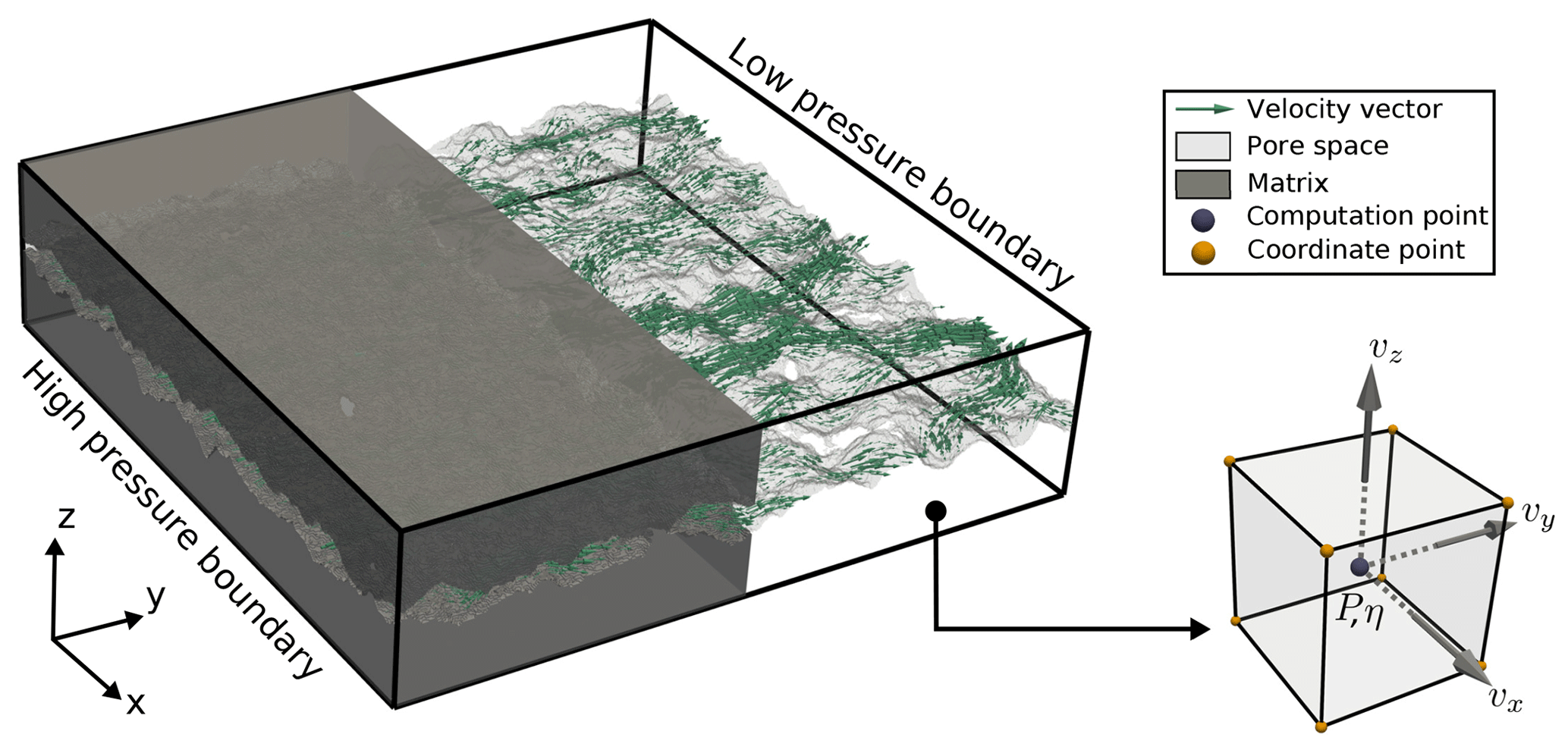
Figure 3 Model setup employed in the numerical simulations. The two boundaries where the pressure gradient is applied are indicated. The green velocity vectors are used for the computation of $\stackrel{\mathrm{‾}}{v}$ and scaled according to their magnitude. The subfigure illustrates the staggered-grid discretization scheme of a single voxel.

2.3 Synthetic fracture dataset

As in situ data of fractures are rarely accessible and limited to the size of drill cores, numerical studies commonly rely on a stochastic generation approach for synthetic fractures (e.g., Brown, 1995; Candela et al., 2009). Here, we numerically generate isotropic self-affine surfaces with a MATLAB script (Kanafi, 2016), which makes use of random theory and fractal modeling techniques (Persson et al., 2004). It uses the standard deviation of surface heights σ_s, the Hurst exponent H, the cutoff length l_c, and the system size L in x and y directions as input parameters to obtain s_u(x,y) and s_l(x,y), which are built from two independent Gaussian random number fields. The code is slightly modified, such that the seeds for the random number generator are prescribed to produce reproducible results. The mean planes (x–y coordinate plane in both cases) of s_u and s_l are separated by varying values of d according to Eq. (5) to simulate different closure stages of the fracture. Since ignoring mechanical deformation is a common practice (Brown, 1987; Méheust and Schmittbuhl, 2000, 2003; Mourzenko et al., 2018), we also assume that both surfaces are in contact at the locations where they overlap. Finally, the data are transferred into a 3-D voxel space of $\mathrm{512}\times \mathrm{512}\times \mathrm{128}$ voxels with a fixed physical voxel size of 0.1 mm, resulting in a model domain of $\mathrm{51.2}\times \mathrm{51.2}\times \mathrm{12.8}$ mm. The relative closure and the effective surface area are computed according to Eqs. (8) and (10), respectively. It is important to note that both quantities are computed only within the effective pore space of the fracture parallel to the direction of the applied pressure gradient because only this contributes to the overall flow. For some configurations, it might be possible to have small amounts of trapped pore space within the fracture, which must be excluded before further numerical treatment. We separate the datasets generated in this study into two groups, each with specific sets of input-parameter combinations and a certain number of realizations (input values are listed in Table 1). The first group is used to analyze the percolation probabilities and determine the parameter boundaries for geometries of group 2, which are later used for numerical flow simulations. To check whether each fracture configuration in group 1 is able to transmit fluids, i.e., if it is percolating or not, we apply a recursive flood-filling MATLAB routine (e.g., Torbert, 2016). Then, the percolation probability p represents the mean value of n fracture realizations built from one specific input parameter combination, such that

$$\begin{array}{}\text{(14)}& p={\displaystyle \frac{\mathrm{1}}{n}}\sum _{i=\mathrm{1}}^n{p}_i\text{, with}{p}_i=\left\{\begin{array}{l}\mathrm{1}\text{if percolating}\\ \mathrm{0}\text{if non-percolating}.\end{array}\right.\end{array}$$

Figure 4 shows the percolation probability as a function of relative closure R, as there was no notable variation with respect to their effective surface areas. Generally, the percolation probability starts reducing from 1 at R≈1 and converges to zero at R≈5. Higher l_c∕L ratios show earlier convergences to their percolation limit, as visible from the two fitted lines for l_c∕L 1 and 1∕16. From the inset plot, it is evident that the contact fraction of all models only depends on the relative closure R; first contact between both walls occurs at $R\ge \mathrm{3}\sqrt{\mathrm{2}}{\mathit{\sigma }}_{\mathrm{a}}$, which is in good accordance with Brown (1987). Following this, we have chosen to limit the fracture geometries for the fluid flow simulations to configurations with R≤1 to (i) exclude non-percolation systems and (ii) limit the effect of the above-mentioned “melting” hypothesis, which intensifies with increasing R. To ensure applicability to nature, the input values for group 2 (see Table 1) are chosen, such that the resulting fracture geometries are classified from “closed” to “open” joints according to Bieniawski (1989). The resulting parameter ranges for fractures in group 2 can be found in Table 2. For the numerical fluid flow simulations, we implemented the following workflow. First, we apply a flood-filling algorithm on the initial 3-D model along the x direction. R and S are calculated on the resulting effective pore space, followed by a numerical permeability estimation, as explained above, in the same direction. Then, we rotate the initial model by 90^∘ in the x–y plane, and the procedure explained above is repeated. In this manner, two-directional permeability values for every fracture are obtained, resulting in a total sum of 12 800 fluid-flow simulations.

Table 1 Minimal and maximal input values for parameters d, σ_s, H, and l_c∕L. n denotes the total number of increments, including minimum and maximum. Subscripts g1 and g2 indicate data for group 1 or 2, respectively. Thus, multiplying the n values of each parameter gives the total number of parameter combinations (6000 for group 1, 320 for group 2). The number of realizations for a set (i.e., the number of different random number seeds used to generate the surfaces with one peculiar parameter combination) are given in the footnotes, resulting in a total of 600 000 and 6400 fracture configurations for groups 1 and 2, respectively.

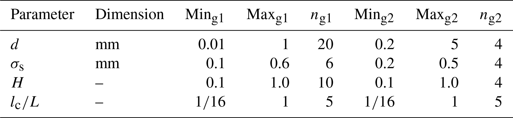
r_g1=100; r_g2=20.

Table 2 Resulting minimal and maximal values for mean aperture ($\stackrel{\mathrm{‾}}{a}$), standard deviation of the aperture field (σ_a), contact fraction (c), relative fracture closure (R), effective surface area (S), and numerical fracture permeability (k_m) for the fracture geometries in group 2.

Figure 4 Percolation probability p (Eq. 14) and the mean fractional amount of contact c as a function of relative closure R for all fracture realization sets of groups 1 and 2. Different shades of blue indicate different l_c∕L ratios as given in the legend, whereas black lines show best fits to the data.

3 Results

3.1 Hydraulic efficiency

In the following section, we present the results of the numerical fluid flow experiments within the geometries of group 2. For this, we normalize the numerically computed permeabilities (k_m) by the permeability predicted by the cubic law (k_cl) with equivalent mean aperture $\stackrel{\mathrm{‾}}{a}$ of the associated effective pore space:

$$\begin{array}{}\text{(15)}& \mathit{\chi }={\displaystyle \frac{k_{\mathrm{m}}}{k_{\mathrm{cl}}}}.\end{array}$$

Consequently, one can use the hydraulic efficiency χ as the correction factor in Eq. (11) to apply the cubic law to rough fractures. In that way, a fracture whose configuration is close to the parallel plates geometry shows excellent hydraulic efficiency with χ close to 1. In the R–S space, the parallel plate fracture configuration exclusively corresponds to a single point with coordinates (0,1). Perfect hydraulic efficiencies (χ=1) were validated by flow simulations in parallel-plate fractures.

The key result of this study, a model that corrects the cubic law in terms of quantified fracture roughness, is proposed in Fig. 5. Due to the complexity of the results, we fitted a regularized surface with a MATLAB function called “gridfit” (D'Errico, 2006) to approximate the solution in R–S space. The function can interpolate scattered data within a prescribed bounding box and a certain amount of smoothing, resulting in a clearer solution image compared to conventional interpolation techniques. Furthermore, to enable an adequate basis for the fitting, the data were cropped above R=1.0 and S=2.5 to provide sufficient data density in R–S space, which reduces the total amount of simulations used for the fitting from 12 800 to 10 292.

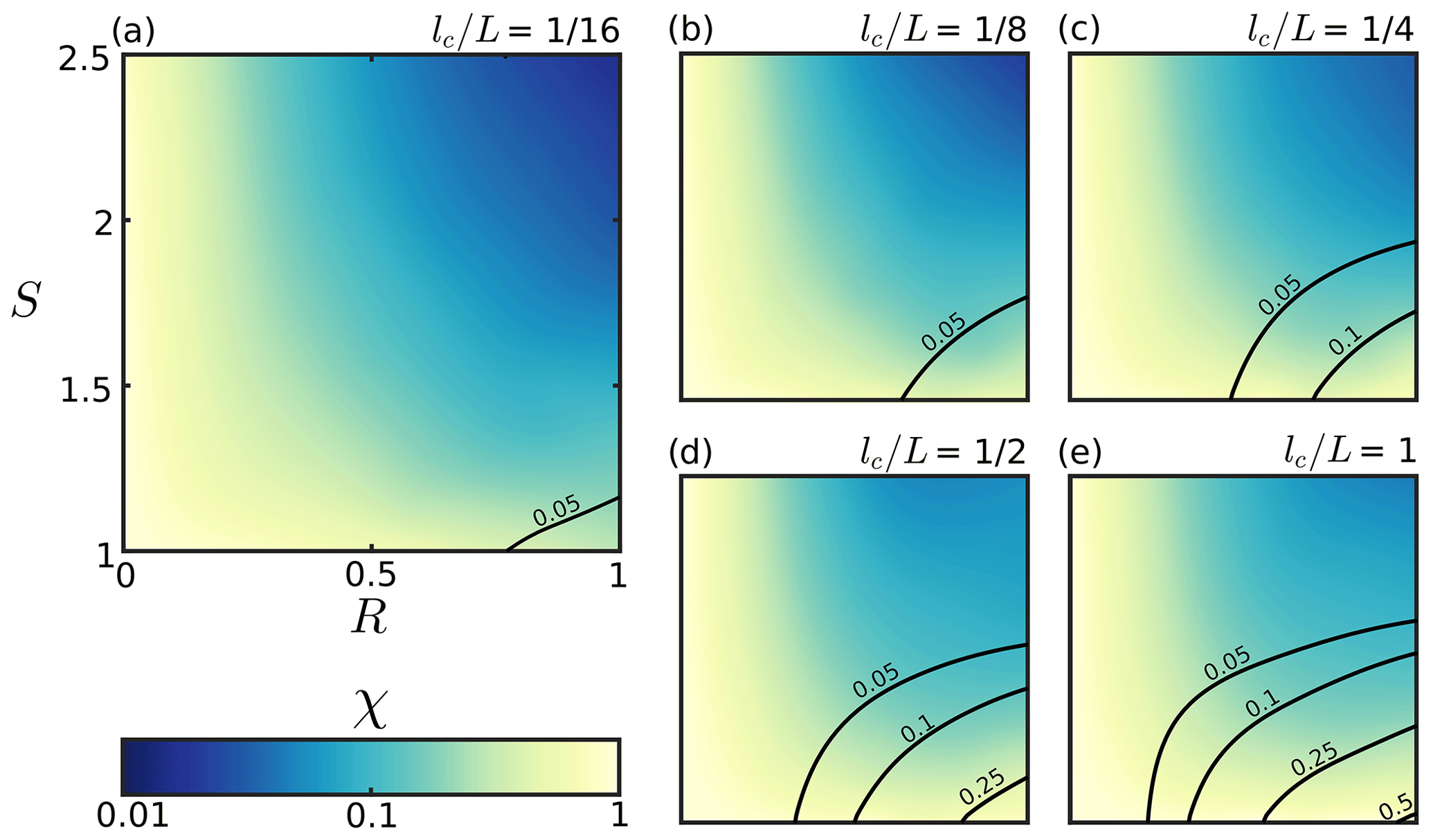
Figure 5 The distribution of the hydraulic efficiency χ for different l_c∕L ratios as a function of R and S. Both axes limits in panel (a) correspond to panels (b)–(e). Dark blue color indicates poor hydraulic efficiency, whereas lighter color shows increasing accordance with the cubic law. The black contour lines indicate the absolute residuals to the fitted surface (compare with Fig. 6).

The results display significant deviations from the cubic law approximation, even for fractures where both surfaces are not in contact (i.e., R≤0.23). We obtain the lowest χ values in regions of high R and S, with a general trend of increasing χ for larger l_c∕L ratios. To investigate the hydraulic efficiency fluctuations for similar fracture configurations, the absolute residuals of the fitted surface from Fig. 5 to the simulated data are computed. As before, we fit a regularized surface through the scattered points from which we extract the displayed contour lines (Fig. 5). They indicate that the goodness of the fit reduces with increasing l_c∕L ratios, especially in the lower right corner. Hence, the non-uniqueness of the data reduces for lower l_c∕L ratios, which can be even better seen in Fig. 6. A regional maximum residual of about 0.2 for fractures with a l_c∕L ratio of 1∕16 enables a more or less unique parametrization refinement, which is not the case for higher l_c∕L ratios. Our finding that low l_c∕L ratios show lower reduced variability is consistent with the results of Méheust and Schmittbuhl (2003).

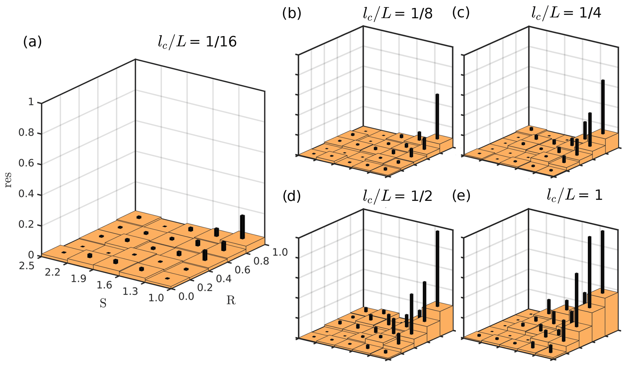
Figure 6 Absolute residual values of the fitted surfaces in Fig. 5 for different l_c∕L ratios as a function of R and S, binned into equally sized boxes. All axes limits in panel (a) correspond to the ones in panels (b)–(e). Orange boxes indicate the mean absolute residual value of the specific bin, whereas the smaller black boxes on top give the maximum absolute residual.

An easy integration of this parametrization refinement into a DFN framework requires a mathematical approximation of the fitted surface shown in Fig. 5a), which was found by the following equation:

$$\begin{array}{}\text{(16)}& \begin{array}{rl}\mathit{\chi }& =\mathrm{1}-\left(\mathrm{0.4809}\tanh \right(\mathrm{0.5139}S)+\mathrm{0.5408})\\ & \cdot \tanh \left({\displaystyle \frac{R}{\mathrm{39.28}\tanh (-\mathrm{2.451}S)+\mathrm{39.47}}}\right).\end{array}\end{array}$$

To predict single-fracture permeability, it is only necessary to know the mean and standard deviation of the aperture field ($\stackrel{\mathrm{‾}}{a}$ and σ_a), the fractional amount of surface contact (c), and the surface area protruding into the void space (sa_f). From these values, R and S are computed to infer the hydraulic efficiency χ with Eq. (16), which is then multiplied by the permeability predicted by the cubic law with aperture $\stackrel{\mathrm{‾}}{a}$ (see Eq. 11). Figure 7 demonstrates the accuracy of Eq. (16) to predict hydraulic efficiencies and accompanying permeabilities for fractures with l_c∕L ratios of 1∕16. To quantify the hydraulic efficiency fluctuations (σ_χ) with respect to its correlation length, we provide a model of the form

$$\begin{array}{}\text{(17)}& {\mathit{\sigma }}_{\mathit{\chi }}=(a\times e^R+b)(c\times \tanh (S)+d),\end{array}$$

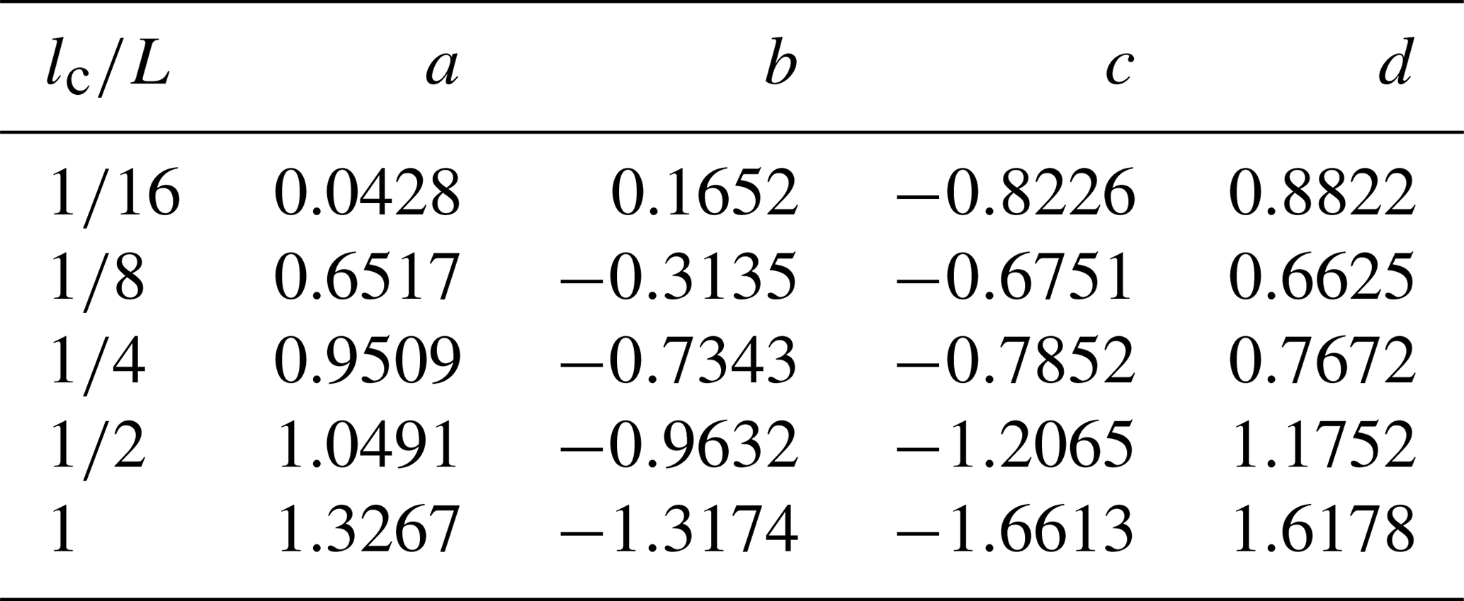
with corresponding parameter values given by Table 3.

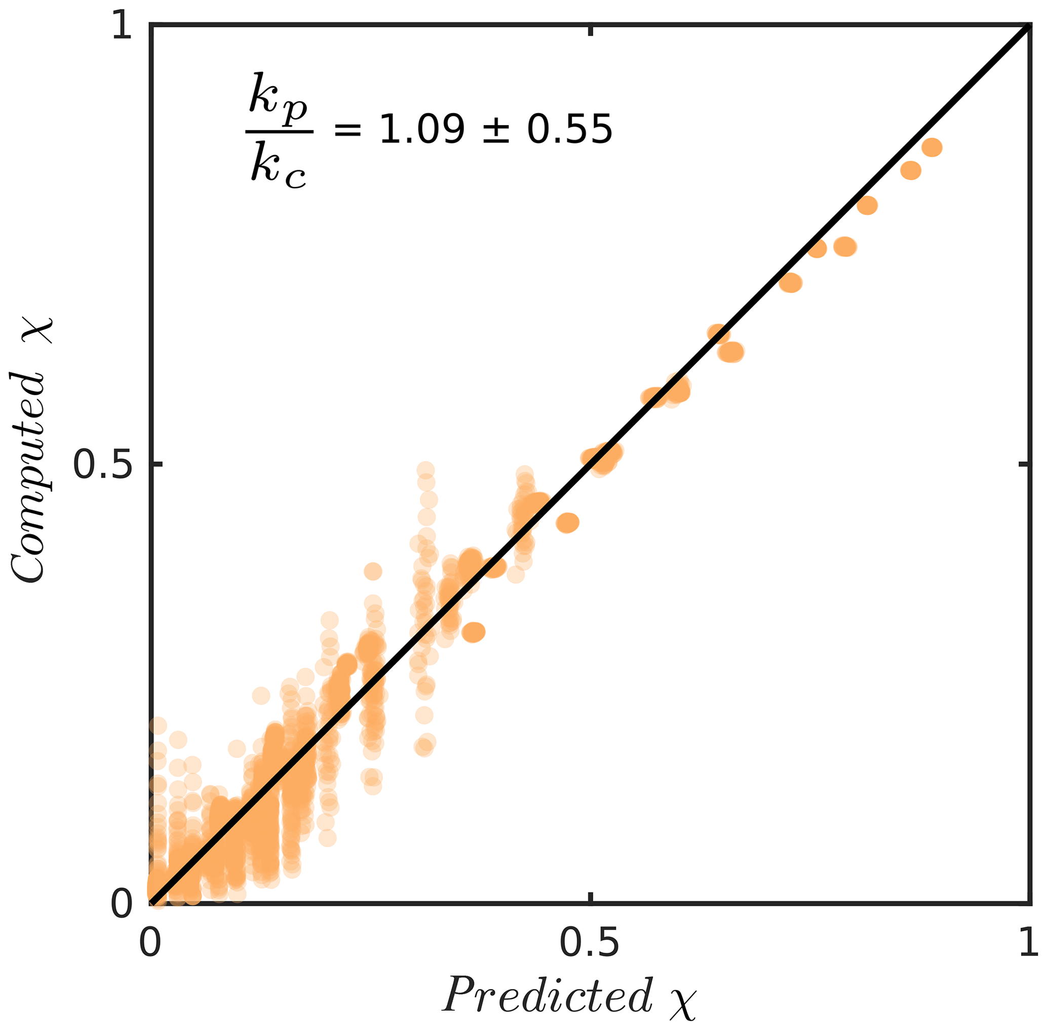
Figure 7 Parity plot of predicted versus computed hydraulic efficiency χ for a total of 2554 fractures with an l_c∕L ratio of 1∕16. The black line indicates the location of perfect parity. Inlet data give the mean and standard deviation of predicted (k_p) over computed (k_c) permeabilities that correspond to all data points in the plot.

Table 3 Coefficients a, b, c, and d of Eq. (17), determined by least-square fitting for fractures with varying l_c∕L ratios.

3.2 Accuracy of the numerical solution

Numerical inaccuracies in solving the Stokes flow equations related to the resolution of the numerical models potentially have an important impact on the results shown here. For numerical permeability estimations of single fractures, the resolution perpendicular to the aperture field is the most crucial part. As the most relevant roughness features are expressed within the uncorrelated region of a fracture (i.e., where l_c=L), it is necessary to examine the numerical error introduced due to resolution loss therein. For that, eight fractures with the size of $\mathrm{4096}\times \mathrm{4096}\times \mathrm{512}$ voxels and a l_c∕L ratio of 1∕16 are generated in the same manner as explained in Sect. 2.3. For each fracture, 16 subsets are drawn that focus uncorrelated regions of the fracture, resulting in subsets of $\mathrm{256}\times \mathrm{256}\times \mathrm{512}$ voxels. By this, the fracture part oriented perpendicular to the applied pressure gradient is over-resolved by a factor of 2. The resolution of these initial models is then consecutively reduced down to $\mathrm{16}\times \mathrm{16}\times \mathrm{32}$ voxels (see inlay of Fig. 8 for a workflow sketch) while maintaining a constant dimensional aspect ratio. The resulting permeability at every stage (k_r) is then compared to the result at maximal resolution (k_max), assuming that this represents the most accurate solution. Finally, we compute the error norm according to

$$\begin{array}{}\text{(18)}& \left|\right|{\mathit{\delta }}_k\left|\right|=\left|{\displaystyle \frac{k_{\mathrm{r}}-k_{max}}{k_{max}}}\right|.\end{array}$$

Ideally, the error norm should get negligible at the highest resolution. Figure 8 shows the mean error norm of a total of 128 uncorrelated fracture subsets as a function of voxel size Δr. A mean error of about 0.01 % at maximal resolution indicates optimal convergence to the most accurate solution, which validates the numerical procedure. The voxel size of the numerical models used in this study (0.1 mm) results in an acceptable mean error of 7.2 %, as indicated in Fig. 8.

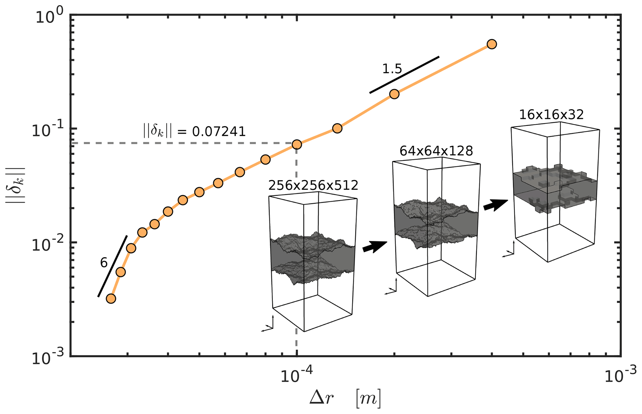
Figure 8 Error norm computed by Eq. (18) as a function numerical voxel size Δr. The orange line depicts the mean error of 128 different fracture subsets discretized with decreasing resolutions. The figure inlay sketches the downsampling procedure: the maximal resolution is consecutively decreased by 16 voxels in the horizontal and 32 voxels in the vertical direction (displayed are the maximal, intermediate, and minimal reduction stages). Dashed gray lines indicate the voxel size and associated error norm of the numerical simulations used to provide the refined single-fracture permeability parameterization. Black lines highlight the convergence rate by showing local slopes as indicated by the attached values.

4 Discussion

Many studies report that the cubic law increasingly deviates with increasing relative fracture closure (Patir and Cheng, 1978; Brown, 1987; Zimmerman and Bodvarsson, 1996), which is usually attributed to the flow channeling around the contact spots within the fracture, introducing an in-plane tortuosity that reduces the permeability. We quantified the deviations from the cubic law due to vertical roughness features (i.e., amplitudes or Hurst exponents; see Fig. 5). The results suggest that with increasing fracture surface area protruding into the fluid phase, more drag force accumulates at the fluid–matrix interface, which resists the flow and leads to reduced permeabilities. It is not possible to capture these vertical variations in the flow field with previous 2-D modeling approaches (e.g., Patir and Cheng, 1978; Brown, 1987; Renshaw, 1995; Zimmerman and Bodvarsson, 1996), which then results in a biased prediction and the need for more parameters to ensure an adequate quantification. Figure 9 highlights this issue by computing the norm $\left|\right|{\mathit{\delta }}_k\left|\right|$ between measured and predicted permeabilities for all fractures in this study. With a mean error of 26.7 %, Eq. (16) delivers a better prediction compared to the mentioned studies.

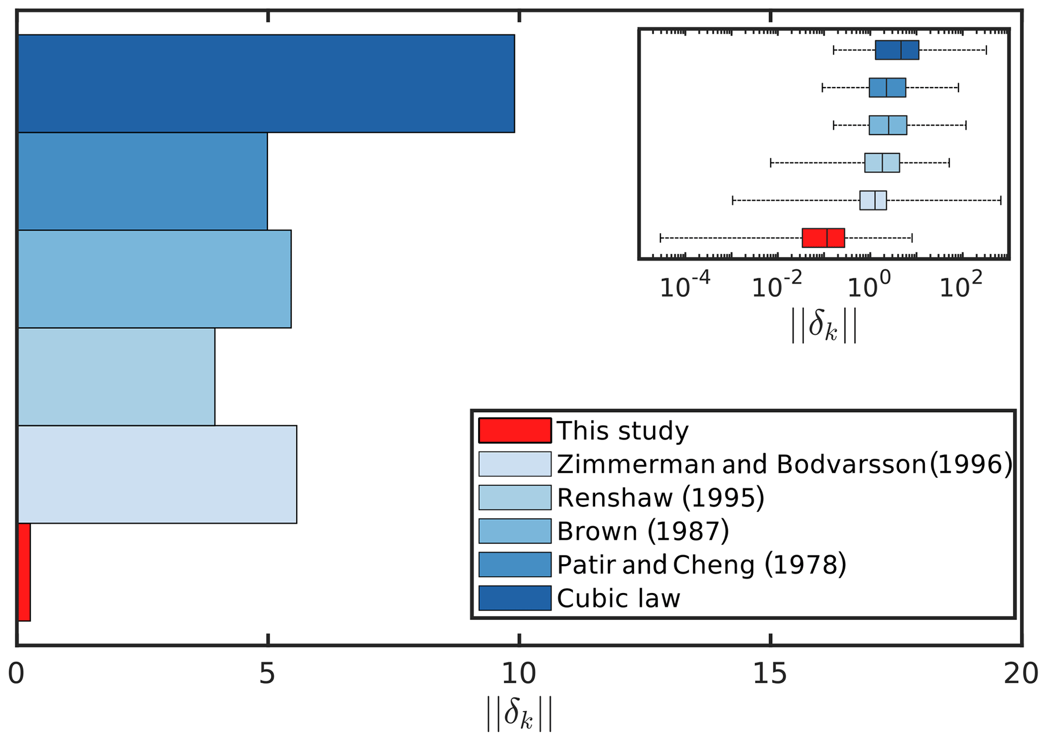
Figure 9 Mean error norm δ_k (see Eq. 18) of all fractures considered in this study for different prediction models. The mean error norm recorded for this study is 0.267. Inlet plot shows box and whisker plots incorporating all outliers, i.e., representing minimum and maximum recorded values.

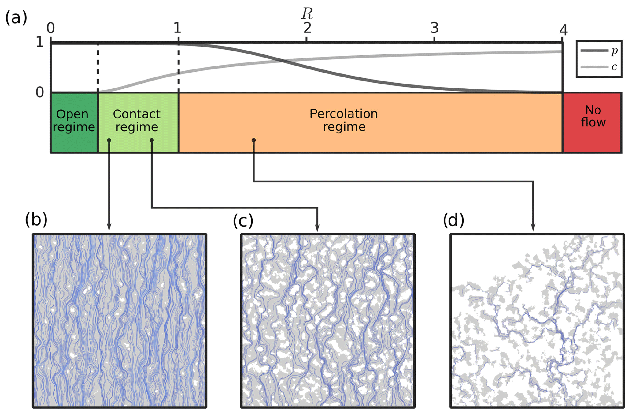
Figure 10 A sketch of the three different closure regimes, indicated as a function of R with corresponding p and c. The lower part of the figure shows three examples of fluid flow simulations from the indicated regimes. The gray shaded area is fracture void space, whereas the white regions indicate contact between both surfaces. Blue lines depict chosen streamlines, approximated from the resulting Stokes velocity vectors.

As already shown by Méheust and Schmittbuhl (2003), the uncertainty for predicting fracture flow is a function of its l_c∕L ratio. Considering flow predictions for uncorrelated fractures (i.e., $l_{\mathrm{c}}/L\ge \mathrm{1}$) is problematic. Blocked pathways connected to the early appearance of the percolation limit (see Fig. 4) or flow-enhancing configurations (χ>1) as also observed by Méheust and Schmittbuhl (2000) are producing substantial variations in their hydraulic efficiencies. With decreasing l_c∕L ratios, the impact of vertical flow tortuosity on its permeability increases relative to the impact of in-plane tortuosity, as both start to act at comparable scales and generally the fractures exhibit larger portions of flow-inhibiting regions compared to flow-enhancing ones (see Méheust and Schmittbuhl, 2000). On the contrary, the fluctuations in the average flow behavior decrease significantly with decreasing l_c∕L ratios. This suggests that predicting hydraulic properties is constrained to fractures whose sizes are significantly greater than their correlation lengths. Theoretically, the correlation length is mainly controlled by shear offset and respective gouge generation (Brown, 1995; Méheust and Schmittbuhl, 2000). With the assumption of a perfectly matched fracture (l_c=0) at its nucleation stage, it is tempting to propose that most natural fractures actually meet the conditions of low l_c∕L ratios and subsequently enable the prediction of their hydraulic properties. However, so far, little is known about naturally existing correlation lengths in fractures, as the imaging of in situ fractures is limited to the size of drill cores. Only Brown (1995) report measurements of l_c by analyzing the power spectral densities of composite topographies for two matched profiles on opposing joint surfaces, shedding some light onto their natural ranges. From a mechanical perspective, correlation lengths that are equal to the size of the fracture seem rather unrealistic, considering that the shear displacement d_s of fractures scales with their length L_f according to $d_{\mathrm{s}}=\mathit{\alpha }{L_{\mathrm{f}}}^{\mathrm{0.5}}$ (Schultz et al., 2008). Using α values between 0.01 and 0.001, which is about the range for Moros joints in Schultz et al. (2008), results in a maximal l_c∕L_f ratio of 0.01. All of that illustrates that further research on fractures correlation lengths is required because the presence of it is omnipresent in most relevant studies (Brown, 1995; Mourzenko et al., 1996; Méheust and Schmittbuhl, 2003; de Dreuzy et al., 2012; Pyrak-Nolte and Nolte, 2016; Mourzenko et al., 2018).

5 Conclusions

To understand the effects of fracture surface roughness on fluid flow, we performed numerical simulations of high-resolution 3-D Stokes flow within fractures for a large synthetic dataset. By consolidating varying asperity amplitudes and roughness scaling within a new quantity, which accounts for the effective increase of surface roughness compared to its parallel plate equivalent, we were able to provide a new way to characterize fracture roughness. By combining the effective surface area with the relative fracture closure, we established a two-parameter characterization scheme that reads similar to a phase diagram. It is utilized to quantify the hydraulic efficiency of single fractures empirically, i.e., the correction factor applied to the current state-of-the-art fracture permeability parametrization (cubic law). Our findings confirm the results of Méheust and Schmittbuhl (2003), and highlight that predicting fracture flow is constrained to scales of at least 16 times larger than the correlation length. The hydraulic efficiency as a function of effective surface area and fracture closure is given by Eq. (16), its variability with respect to the correlation length is given by Eq. (17) and Table 3, whereas an overall numerical error of 7.2 % has to be considered. Ultimately, we used the percolation probability and contact fractions to classify three different closure regimes (see Fig. 10 for a sketch) that differ in terms of their hydraulic interpretation:

• i.

  The open regime defines fractures whose surface walls are not in contact with each other (e.g., unconfined dilatant or karstified fractures). In this regime, we generally observe a good agreement of the cubic law with hydraulic efficiency between 70 % and 100 %, and only extreme roughness configurations (e.g., needle-shaped mineral coatings) result in larger deviations.

• ii.

  The contact regime is characterized by fractures exhibiting a rapidly decreasing hydraulic efficiency from 70 % to 10 %, up to 1 % in extreme cases, which is caused by strong three-dimensional channeling due to surface roughness and increasing fracture closure. Likely, this regime is most suitable for subsurface conditions, as a certain amount of contact between both fracture surfaces is required to withstand confining pressures.

• iii.

  The percolation regime incorporates fracture configurations that do not percolate at all due to blocked fluid pathways. Here, we do not incorporate fluid flow data, but it is plausible that the hydraulic efficiency is very poor with a maximum of 25 %, which will quickly converge to 0 % due to the effect of decreasing percolation probability with further closure. We observe the no-flow boundary at R≈6.

Our results generally help to understand the hydraulic response induced by different types of fracture geometries and refine the parametrization of single-fracture permeability given by the cubic law. Moreover, the developed quantification scheme allows monitoring and parametrizing the hydraulic and geometric evolution of fractures during aperture field-shaping processes. This parametrization can easily be incorporated in a DFN modeling framework to investigate the hydraulic responses at reservoir scales, assuming that the minimal correlation length is no longer than 1∕16 of the reservoir size. If DFNs of scales close to the correlation length are considered, fluctuations in the average flow behavior are expected. This can modify network-scale flow connectivity and thus requires additional concepts to compute permeabilities (e.g., de Dreuzy et al., 2012).