Reproducing pyroclastic density current deposits of the 79 CE eruption of the Somma–Vesuvius volcano using the box-model approach

We use PyBox, a new numerical implementation of the box-model approach, to reproduce pyroclastic density current (PDC) deposits from the Somma–Vesuvius volcano (Italy). Our simplified model assumes inertial flow front dynamics and mass deposition equations and axisymmetric conditions inside circular sectors. Tephra volume and density and total grain size distribution of EU3pf and EU4b/c, two well-studied PDC units from different phases of the 79 CE Pompeii eruption, are used as input parameters. Such units correspond to the deposits from variably dilute, turbulent PDCs. We perform a quantitative comparison and uncertainty quantification of numerical model outputs with respect to the observed data of unit thickness, inundation areas and grain size distribution as a function of the radial distance to the source. The simulations consider (i) polydisperse conditions, given by the total grain size distribution of the deposit, or monodisperse conditions, given by the mean Sauter diameter of the deposit; (ii) axisymmetric collapses either covering the whole 360^∘ (round angle) or divided into two circular sectors. We obtain a range of plausible initial volume concentrations of solid particles from 2.5 % to 6 %, depending on the unit and the circular sector. Optimal modelling results of flow extent and deposit thickness are reached on the EU4b/c unit in a polydisperse and sectorialized situation, indicating that using total grain size distribution and particle densities as close as possible to the real conditions significantly improves the performance of the PyBox code. The study findings suggest that the simplified box-model approach has promise for applications in constraining the plausible range of the input parameters of more computationally expensive models. This could be done due to the relatively fast computational time of the PyBox code, which allows the exploration of the physical space of the input parameters.

1 Introduction

The increased availability of numerical models capable of reproducing, with various degrees of simplification, the dynamics of pyroclastic flows (see Sulpizio et al., 2014, for a review) provided geoscientists and civil authorities with new valuable tools for better understanding natural phenomena and for more accurate hazard assessments. Several modelling approaches have been developed over the past years for pyroclastic density currents (PDCs), from simplified 1D kinetic models (Malin and Sheridan, 1982; Sheridan and Malin, 1983; Dade and Huppert, 1995b, 1996; Bursik and Woods, 1996; Doyle et al., 2010; Esposti Ongaro et al., 2016; Fauria et al., 2016) up to more complex, 2D depth-averaged models (Patra et al., 2005, 2020; Charbonnier and Gertisser, 2009; Kelfoun et al., 2009, 2017; Tierz et al., 2018; de'Michieli Vitturi et al., 2019) and computationally expensive but physically realistic 2D (axisymmetric) and 3D models (Esposti Ongaro et al., 2002, 2007, 2012, 2019; Todesco et al., 2002, 2006; Neri et al., 2003; Dufek and Bergantz, 2007; Dufek et al., 2015; Dufek, 2016).

Although the 1D kinetic approaches cannot capture the multidimensional features of dynamics, they represent an important tool for several purposes. Firstly, it is practical to rely on simplified and fast numerical codes, which can be run 10⁴–10⁶ times without an excessive computational expense, in order to produce statistically robust probabilistic hazard maps (Neri et al., 2015; Bevilacqua et al., 2017; Aravena et al., 2020). Furthermore, since 2D or 3D multiphase models require high computational times, often on the order of days or weeks for a single simulation, it is convenient to use simplified approaches, such as the box model, in order to constrain the input space (Ogburn and Calder, 2017; Bevilacqua et al., 2019a). Finally, extensively testing the numerical models in a statistical framework and evaluating the difference between model outputs and actual observations also allows estimation of the effect of the various modelling assumptions under uncertain input conditions (e.g. Patra et al., 2018, 2020; Bevilacqua et al., 2019b). Model uncertainty is probably the most difficult class of epistemic uncertainty to evaluate robustly, but it is indeed a potentially large component of the total uncertainty affecting PDC inundation forecasts.

In this paper, we test the suitability of the box-model approach, as implemented numerically in the PyBox code (Biagioli et al., 2019), by quantifying its performance when reproducing some key features of the well-characterized PDC deposits from one of the best studied and documented volcanic events: the 79 CE eruption of the Somma–Vesuvius (SV) volcano. The box model is able to describe the main features of large-volume (VEI 6 to 8; Newhall and Self, 1982), low-aspect-ratio ignimbrites, whose dynamics are dominantly inertial (Dade and Huppert, 1996; Giordano and Doronzo, 2017), although there was some debate on the mechanism of flow emplacement in that case study (Dade and Huppert, 1997; Wilson, 1997). In general, thick density currents are able to propagate inertially even on flat topographies, and the effect of friction is usually negligible. Low-aspect-ratio ignimbrites or flows produced can generally be modelled as “inertial PDCs” for most of their run-out (de'Michieli Vitturi et al., 2019). However, the model has never been tested against PDC generated by VEI 5 Plinian eruptions (Shea et al., 2011). The procedure involves the calculation of the difference between model output and field data in terms of (i) thickness profile, (ii) areal invasion overlapping and (iii) grain size (GS) volume fractions at various distances from the source (see, for example, Dade and Huppert, 1996; Kelfoun, 2011; Charbonnier et al., 2015). Tierz et al. (2016a, b) and Sandri et al. (2018) proposed a quantification of the uncertainty derived from the energy cone approach that relies on the comparison between invaded area and maximum run-out of model output and field data. Our approach aims at the more detailed comparison of physical parameters (especially thickness and grain sizes), which allows a further investigation of the strengths and limitations of the PyBox model when used to simulate different PDC types.

2 Numerical model and data sources

2.1 The box-model approach and the PyBox code

PyBox is a numerical implementation of the box-model integral formulation for axisymmetric gravity-driven particle currents based on the pioneering work of Huppert and Simpson (1980). The theory is detailed in Bonnecaze et al. (1995) and Hallworth et al. (1998). The volume extent of gravity currents is approximated by an ideal geometric element, called “box”, which preserves its volume and geometric shape class and only changes its height∕base ratio through time (Fig. 1). The box does not rotate or shear but only stretches out as the flow progresses. In this study the geometric shape of the box is assumed to be a cylinder; i.e. we assume axisymmetric conditions.

Figure 1 (a) Schematic diagram of an inertial gravity current with a depth h_c, flow front velocity u_c and density ρ_c in an ambient fluid of density ρ₀ (modified from Roche et al., 2013); (b) evolution of channelized currents through a series of equal-area rectangles, according to the model (hence the name “box model”).

The model describes the propagation of a turbulent particle-laden gravity current, i.e. a homogeneous fluid with suspended particles. Inertial effects are assumed to dominate with respect to viscous forces and particle–particle interactions. Particle sedimentation is modelled and modifies the current inertia during propagation. In this study we assume the classical dam break configuration, in which a column of fluid instantaneously collapses and propagates, under gravity, in a surrounding atmosphere with uniform density ρ_atm. Other authors (Bonnecaze et al., 1995; Dade and Huppert, 1995a, b, 1996) have instead considered gravity currents produced by the constant flux release of dense suspension from a source. Our approach does not assume constant stress acting on the basal area as in Dade and Huppert (1998). Constant stress dynamics have been explored in literature, and they can lead to different equations if the basal area grows linearly or with the square of the radius (Kelfoun et al., 2009; Kelfoun, 2011; Ogburn and Calder, 2017; Aspinall et al., 2019). Bevilacqua (2019) provides a brief derivation of various examples of box-model equations either under constant stress or sedimentation.

Our model consists of a set of ordinary differential equations, which provide the time evolution of flow front distance from the source, l(t), together with the current height h(t) and the solid particle volume fraction $({\mathit{\epsilon }}_i{)}_{i=\mathrm{1},\mathrm{\dots },N}$, N being the number of particle classes considered. The volume fractions refer to a constant volume of the mixture flow, not reduced by the deposition.

PDCs are driven by their density excess with respect to the surrounding air: the density of the current ρ_c is defined as the sum of the density of an interstitial gas, ρ_g and the bulk densities of the pyroclasts carried by the flow, $({\mathit{\rho }}_i^s{)}_{i=\mathrm{1},\mathrm{\dots },N}$. In this study we assume ρ_atm≠ρ_g i.e. the interstitial gas is hotter than surrounding atmosphere, differently from Neri et al. (2015) and Bevilacqua et al. (2017). The code allows ρ_atm>ρ_g, but thermal properties remain constant for the duration of the flow. A proper way to express the density contrast between the current and the ambient fluid is given by the reduced gravity g^′, which can be rewritten in terms of the densities and the volume fractions described above (see Biagioli et al., 2019). That said, we make some additional simplifications. First, we assume that the mixture flow regime is incompressible and inviscid, since we assume that the dynamics of the current are dominated by the balance between inertial and buoyancy forces. The assumption of incompressibility implies that the initial volume V₀ remains constant. Moreover, we assume that, within the current, turbulent mixing produces a vertically uniform distribution of particles. The particles are assumed to sediment out of the current at a rate proportional to their constant terminal (or settling) velocity $(w_i^s{)}_{i=\mathrm{1},\mathrm{\dots },N}$ and, once deposited, they cannot be re-entrained by the flow; the converse was explored in Fauria et al. (2016). Finally, surface effects of the ambient fluid are neglected.

Under these hypotheses, the box model for particle-laden gravity currents states that the velocity of the current front (u) is related to the average depth of the current (h) by the von Kármán equation for density currents $u=\mathit{\text{Fr}}{\left(g^{\prime }h\right)}^{\frac{\mathrm{1}}{\mathrm{2}}}$, where Fr is the Froude number, a dimensionless ratio between inertial and buoyancy forces (Benjamin, 1968; Huppert and Simpson, 1980) and g^′ is the reduced gravity. In addition, we assume that particles can settle to the ground and this process changes the solid particle fractions $({\mathit{\epsilon }}_i{)}_{i=\mathrm{1},\mathrm{\dots },N}$.

The box model for axisymmetric currents thus reads

$$\begin{array}{}\text{(1)}& {\displaystyle }& {\displaystyle \frac{\mathrm{d}l}{\mathrm{d}t}}=\mathit{\text{Fr}}{\left(g^{\prime }h\right)}^{\frac{\mathrm{1}}{\mathrm{2}}},\text{(2)}& {\displaystyle }& {\displaystyle }{l}^{\mathrm{2}}h=l_{\mathrm{0}}^{\mathrm{2}}{h}_{\mathrm{0}},\text{(3)}& {\displaystyle }& {\displaystyle \frac{\mathrm{d}\left({\mathit{\epsilon }}_i\right)}{\mathrm{d}t}}={\displaystyle \frac{w_i^s{\mathit{\epsilon }}_i}{h}}\forall i=\mathrm{1},\mathrm{\dots },N.\end{array}$$

By solving these equations, we computed the amount of mass loss by sedimentation, per unit area and per time step, for each particle class. The thickness profile of the ith particle class is the ratio of the ith deposited mass to the ith solid density multiplied by the packing fraction α measured in the deposit. More details on the numerical solver are provided in Appendix A.

In the calculation of the region invaded by a PDC, first we calculate the maximum flow run-out over flat ground, i.e. the distance at which ρ_c=ρ_atm. The flow stops propagating when the solid fraction becomes lower than a critical value, and, although not modelled, in nature the remaining mixture of gas and particles lifts off, possibly generating a phoenix cloud if hot gas is assumed. In the case of monodisperse systems there are analytical solutions for the maximum flow run-out (Bonnecaze et al., 1995; Esposti Ongaro et al., 2016; Bevilacqua, 2019). Then, once a vent location is set, we assess the capability of topographic reliefs to block the current. In particular, the invasion areas are obtained by using the so-called energy-conoid model, based on the assumption of non-linear, monotonic decay of flow kinetic energy with distance (Neri et al., 2015; Bevilacqua, 2016; Esposti Ongaro et al., 2016; Bevilacqua et al., 2017; Aspinall et al., 2019; Aravena et al., 2020). In more detail, we compare the kinetic energy of the current front and the potential energy associated with the obstacles encountered. In this approach we are neglecting returning waves. When investigating the current flow on complex topographies, we finally consider that the flow may start from positive elevation or encounter upward slopes after downward slopes. In this case, we compare the kinetic energy at a given distance from the vent and the difference in level experienced by the current with respect to the minimum elevation previously run into.

In the PyBox code, the main input parameters are summarized by (a) the total collapsing volume (expressed in terms of the dimension of the initial cylinder or rectangle with height=h₀ and radius/base=l₀); (b) the initial concentration of solid particles, subdivided (for polydisperse simulations) into single particle volumetric fractions (ε₀), with respect to the gas; (c) the density of single particles ρ_s; (d) ambient air density (${\mathit{\rho }}_{\text{atm}}=\mathrm{1.12}\mathrm{kg}{\mathrm{m}}^{-\mathrm{3}}$) and gravity current temperature; (e) Froude number of the flow, experimentally measured by Esposti Ongaro et al. (2016) as Fr=1.18; and (f) gravity acceleration ($g=\mathrm{9.81}\mathrm{m}{\mathrm{s}}^{-\mathrm{2}}$). With respect to points (b) and (c), more details are provided in Sect. 3.2.

2.2 The EU3pf and EU4b/c units from the 79 CE eruption of SV

The 79 CE eruption of SV volcano (Fig. 2a) involved a complex sequence of fallout and PDC phases, resulting in the deposition of a sequence of eruptive units (EUs; Cioni et al., 1992). The EU3pf and EU4b/c units (Fig. 2b) represent the two main PDC deposits, which have been traced over a large area around the volcano and characterized for their most relevant physical parameters (Gurioli et al., 2010; Cioni et al., 2020).

Figure 2 (a) Location of the Somma–Vesuvius volcano. Coordinates are expressed in the UTM WGS84-33N system. (b) The EU3pf unit (Cioni et al., 2020); (c) the EU4 unit (Cioni et al., 2020). In (b), solid lines are the limits between EUs, dashed lines are the limits between levels (a, b and c) and dotted lines are lithofacies stratifications. Lithofacies terminology is derived from Branney and Kokelaar (2002): //LT – “plane-parallel lapilli tuff”; mLT – “massive lapilli tuff”; xsLT – “cross-stratified lapilli tuff”; mL – “massive lapillistone”; and mT_accr – “massive tuff with accretionary lapilli”. Service layer credit source: Esri, DigitalGlobe, GeoEye, Earthstar Geographics, CNES/Airbus DS, USDA, USGS, AeroGRID, IGN and the GIS User Community

The EU3pf unit records the phase of total column collapse closing the Plinian phase of the eruption. This is ca. 1 m thick on average, radially dispersed up to 10 km from the vent area and moderately controlled by local topography. The variability of vertical and lateral facies (Gurioli, 1999; Gurioli et al., 1999) are probably related to local variation in turbulence, concentration and stratification of the current. Median clast size gradually decreases from proximal to distal locations, and the coarsest deposits, generally present as breccia lenses in the EU3pf sequence, are located within paleo-depressions. Gurioli et al. (1999) showed that the deposits reflect different topographic situations in different sectors around the volcano. South of SV the relatively smooth paleo-topography only locally affected the overall deposition of this PDC. In the eastern sector of SV, the interaction of the current with the ridge representing the remnants of the old Mount Somma caldera (Fig. 2a) possibly triggered a general increase in the current turbulence and velocity and a more efficient air ingestion, which resulted in the local deposition of a thinly stratified sequence. To the west of SV, the presence of a breach in the caldera wall and of an important break in slope in the area of Piano delle Ginestre (Fig. 2a), possibly increased deposition from the PDC, producing a large, several metres thick depositional fan toward the sea-facing sectors (like in Herculaneum; Fig. 2a). In the northern sector of SV, the deeply eroded paleo-topography, with many radial valleys cut on steep slopes, favoured the development within the whole current of a fast-moving, dense basal underflow able to segregate the coarse, lithic material and to deposit thick lobes in the main valleys and of a slower and more dilute portion travelling and depositing thin, stratified beds also on morphological highs.

EU4 records a subsequent phase of the eruption and was related by Cioni et al. (1999) to the onset of the caldera collapse. This complex unit has been subdivided into three distinct layers (Cioni et al., 1992): a thin basal fallout layer (EU4a), a PDC deposit derived from the collapse of the short-lived column that emplaced the EU4a layer (EU4b), and the products of the co-ignimbritic plume mainly derived by ash elutriation from the current that deposited EU4b (EU4c). Gurioli (1999) illustrates how the EU4 unit has additional complications, since it actually presents a second fallout bed (EU4a2) interlayered within the level EU4b. This fallout bed can be clearly recognized only in distal sections of the southern sector, while in the north and in the west it is represented by a discontinuous horizon of ballistic ejecta. Level EU4a2 divides level EU4b into two parts, which are approximately two-thirds (the lower one) and one-third (the upper one) of the total thickness of level EU4b (Gurioli, 1999). Run-out of the EU4b PDC is one of the largest run-outs observed for the SV PDCs; to the south it was deposited up to ≈20 km from vent area (Gurioli et al., 2010). This unit has been extensively studied by Gurioli (1999), who highlighted that the high shear rate exerted by the EU4b is clearly evidenced by the formation of traction carpet bedding and local erosion of the pumice-bearing layer of the underlying EU4a. The EU4b deposit can be interpreted as being derived from a short-lived sustained, unsteady, density-stratified current. From a sedimentological point of view, EU4b shows clear vertical grain size and textural variations, from cross-bedded, fine-lapilli to coarse-ash laminae at the base up to a massive, fine-ash-bearing, poorly sorted, matrix-supported bed at the top (Gurioli, 1999). During deposition of EU4b, ash elutriated from the current formed a convective plume dispersed from the prevailing winds in a south-eastern direction, which deposited EU4c mainly by fallout. The clear field association of these two deposits (indicated as EU4b/c) gives here the uncommon possibility to evaluate with a larger accuracy two of the most important PDC source parameters: erupted volume and total grain size distribution (TGSD).

3 Methods

3.1 Model input parameters and field data for comparison

The main properties of the EU3pf and EU4b/c units – thicknesses, total volume, maximum run-out and TGSD – have been calculated in Cioni et al. (2020) and partially processed to fit with PyBox input requirements. Densities of single grain sizes and emplacement temperatures of PDCs (T=600 K for both EU3pf and EU4) are derived from Barberi et al. (1989) and Cioni et al. (2004). Total volume, TGSD, densities and temperature obtained from field data are used as the main inputs of PyBox. The model produces several outputs: (i) mean unit thickness as a function of the radial distance from the source, (ii) inundated area and (iii) grain size distribution as a function of radial distance from the source. All these outputs are finally compared to the corresponding field data. The initial volumetric fraction ε₀ of the solid particles over the gas is the main tuning parameter that is explored to fit the outputs with the field data. This procedure is repeated under monodisperse and polydisperse conditions and by performing round-angle axisymmetric collapses or sectorialized collapses, i.e. divided into two circular sectors with different input parameters.

3.1.1 Thickness, maximum run-out and volumes

Cioni et al. (2020) recently revised and elaborated on a large amount of field data from EU3pf and EU4b/c (106 and 102 stratigraphic sections, respectively), tracing detailed isopach maps (Fig. 3a and b) and defining the maximum run-out distance (the ideal 0 m isopach) and the related uncertainty. Given the objective difficulty in tracing the exact position of a 0 m isopach for the deposit of a past eruption, Cioni et al. (2020) proposed to define three different outlines of PDC maximum run-outs, namely the “5th percentile”, “50th percentile” and “95th percentile” (called maximum run-out lines, MRLs), based on the uncertainty associated with each segment of the proposed 0 m isopach. The MRLs of EU3pf and EU4b are shown in Fig. 3c and d, respectively.

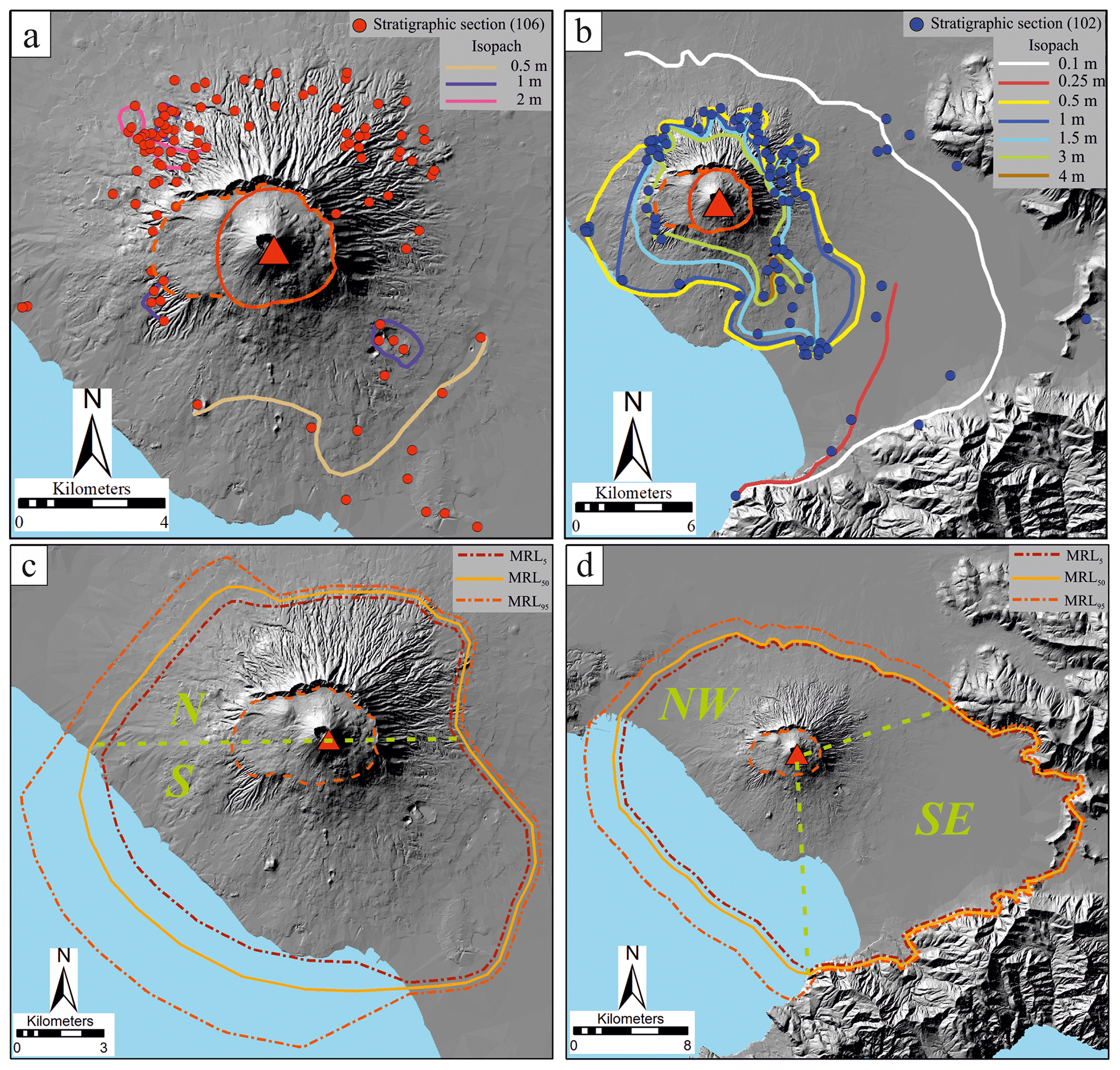
Figure 3 Thicknesses and isopach lines for the (a) EU3pf and (b) EU4b/c units; MRLs of the (c) EU3pf and (d) EU4b/c units. Inferred position of 79 CE vent (red triangle) and SV caldera outline (dark orange dashed line) after Tadini et al. (2017). Light green dashed lines delimit the sectors (N–S for EU3pf and NW–SE for EU4) of the different column collapses. Background DEM from Tarquini et al. (2007).

Table 1 Volume of the EU3pf and EU4b/c units.

Cioni et al. (2020) also calculated the volumes of both EU3pf and EU4b/c, using these maps to derive a digital elevation model of the deposits with the triangular irregular network (TIN) method (Lee and Schachter, 1980). In this study, we considered volume estimations (Table 1) related to the MRL₅₀, the 50th percentile of the maximum run-out distance.

Given the asymmetric shape of unit EU4b/c and, partially, of unit EU3pf, we have also calculated the volumes dividing each unit into two circular sectors: N and S for EU3pf; NW and SE for EU4b/c. These subdivisions have also been used to calculate the related TGSDs (see Sect. 3.1.3) and to perform sectorialized simulations (see Sect. 4). Figure 3c and d display the different sectors for both EU3pf and EU4b/c for which different volumes have been calculated.

3.1.2 Density data

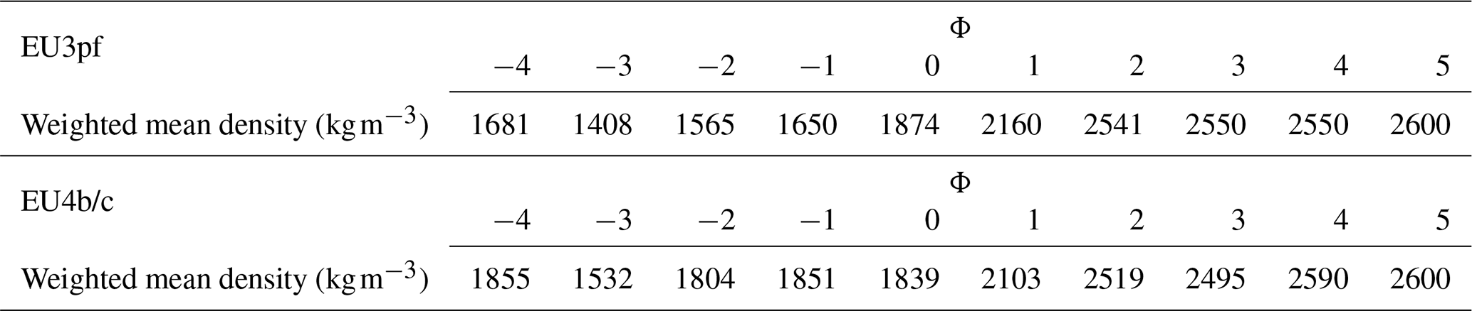
In order to provide density values for each GS, we used the mass fractions of the different components (juveniles, lithics and crystals – see Table S1 in the Supplement) calculated by Gurioli (1999). Such values were associated with the averaged density measurements for these three components presented in Barberi et al. (1989), through which we extrapolated the weighted mean (with respect to mass fraction) density of each grain size class for both EU3pf and EU4b/c units (Table 2).

Table 2 Calculated mean densities for each grain size for both the EU3pf and EU4b/c units.

3.1.3 Grain size data: total grain size distribution and mean Sauter diameter (MSD)

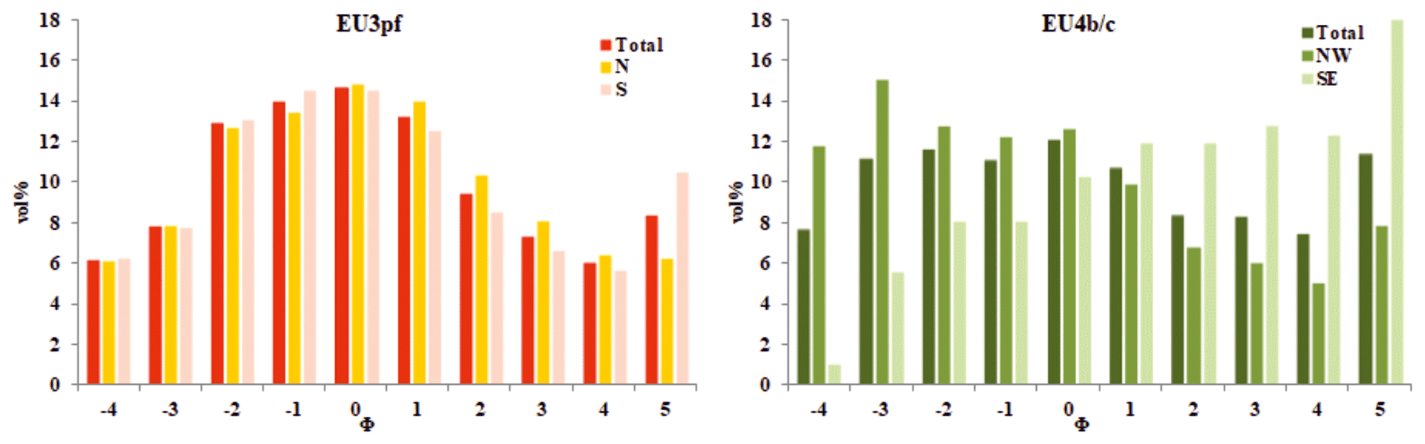
The TGSD estimations are necessary to do simulations under polydisperse conditions. The present version of PyBox takes as input the volumetric TGSD (i.e. in terms of volumetric percentages), while TGSD data from Cioni et al. (2020) are in weight percentages. These latter values have been therefore converted into volumetric percentages by considering the above-mentioned densities (Table 2). Figure 4 displays the volumetric TGSDs employed for EU3pf (total, N and S) and the EU4b/c (total, NW and SE).

Figure 4 Volumetric total grain size distributions for the EU3pf and EU4b/c units.

In the simulations under monodisperse conditions, we used the value of mean Sauter diameter (MSD) of the volumetric TGSD (e.g. Neri et al., 2015). According to Fan and Zhu (1998), the Sauter diameter of each particle class size is also called d₃₂ (see also Breard et al., 2018), and it is the diameter of a sphere having the same ratio of external surface to volume as the particle, which is given by

$$\begin{array}{}\text{(4)}& d_{\mathrm{32}}={\displaystyle \frac{\mathrm{6}V}{S}}={\displaystyle \frac{d_{\mathrm{v}}^{\mathrm{3}}}{d_{\mathrm{s}}^{\mathrm{2}}}},\end{array}$$

where V is the particle volume, S is the particle surface, d_v is the diameter of a sphere having the same volume as the particle and d_s is the diameter of a sphere having the same external surface as the particle. In order to obtain a value for the MSD instead, given a deposit sample divided into N grain size classes, we have initially calculated the number of particles of each grain size $i=\mathrm{1},\mathrm{\dots },N$, that is

$$\begin{array}{}\text{(5)}& n_i={\displaystyle \frac{V_i}{\frac{\mathrm{4}}{\mathrm{3}}\mathit{\pi }{r}_i^{\mathrm{3}}}},\end{array}$$

where V_i is the cumulative volume of the ith grain size class, and r_i is the radius of the ith grain size. The mean MSD is finally derived as

$$\begin{array}{}\text{(6)}& \text{MSD}\left(\mathrm{\Phi }\right)=-{\log }_{\mathrm{2}}\left({\displaystyle \frac{\sum _{i=\mathrm{1}}^N{n}_i{d}_i^{\mathrm{3}}}{\sum _{j=\mathrm{1}}^N{n}_j{d}_j^{\mathrm{2}}}}\right),\end{array}$$

where d_i and d_j are the diameters of, respectively, the ith and jth grain sizes.

Table 3 summarizes the calculated MSDs for the studied units (in Φ), along with the corresponding density values (obtained interpolating those in Table 2).

Table 3 MSD values and related densities for the different units studied.

3.2 Comparison between field data and simulation outputs

Since the PyBox code assumes axisymmetric conditions, the thickness outputs are equal along all the radial directions of the collapse and only vary as a function of the distance to the source. These output data were compared with the mean radial profiles of unit thickness (for both EU3pf and EU4b/c) as derived from the digital models of deposit in Cioni et al. (2020). For building the radial profiles, the average thickness was estimated over concentric circles drawn with a 100 m step of distance. The radial thickness profiles were drawn starting from a distance of 3 km from the vent, as no thickness data are available for sites closer than 3 km. We excluded from our analyses the portions of the circles located in marine areas due to the lack of reliable data. In order to describe the variation range of the thicknesses of the deposits, we are providing minimum and maximum thicknesses along each circle in Appendix B (Fig. A1).

Concerning the inundation area, the methodology adopted is similar to the one used by Tierz et al. (2016b) and relies on the approach described by Fawcett (2006) and implemented by Cepeda et al. (2010) for landslide deposit back-analysis. This method is based on the quantification of the areal overlapping between the measured deposit (true classes) and the modelled deposit (hypothesized classes) (Fig. 5). In particular, we quantify (a) the areal percentage of the model intersecting the actual deposit (true positive – TP); (b) the areal percentage of the model overestimating the actual deposit (false positive – FP); and (c) the percentage of the model underestimating the actual deposit (true negative – TN). More precisely,

$$\begin{array}{ll}{\displaystyle }\text{TP}& {\displaystyle }=\left({\displaystyle \frac{\text{AreaSim}\cap \text{AreaDep}}{\text{AreaSim}\cup \text{AreaDep}}}\right)\times \mathrm{100},\\ {\displaystyle }\text{FP}& {\displaystyle }=\left({\displaystyle \frac{\text{AreaSim}\setminus \text{AreaDep}}{\text{AreaSim}\cup \text{AreaDep}}}\right)\times \mathrm{100},\\ {\displaystyle }\text{TN}& {\displaystyle }=\left({\displaystyle \frac{\text{AreaDep}\setminus \text{AreaSim}}{\text{AreaSim}\cup \text{AreaDep}}}\right)\times \mathrm{100}.\end{array}$$

In statistical literature, the true positive value is also called the Jaccard index of similarity (Tierz et al., 2016b; Patra et al., 2020). While the TP, TN and FP approach, and in general the Jaccard index, focus on areal overlapping, other metrics can specifically focus on the distance between the boundaries of the inundated areas, i.e. the Hausdorff distance, detecting and comparing channelized features in the deposit (Aravena et al., 2020). However, PyBox is not specifically aimed at the replication of such features, and we focus on the areal overlapping properties.

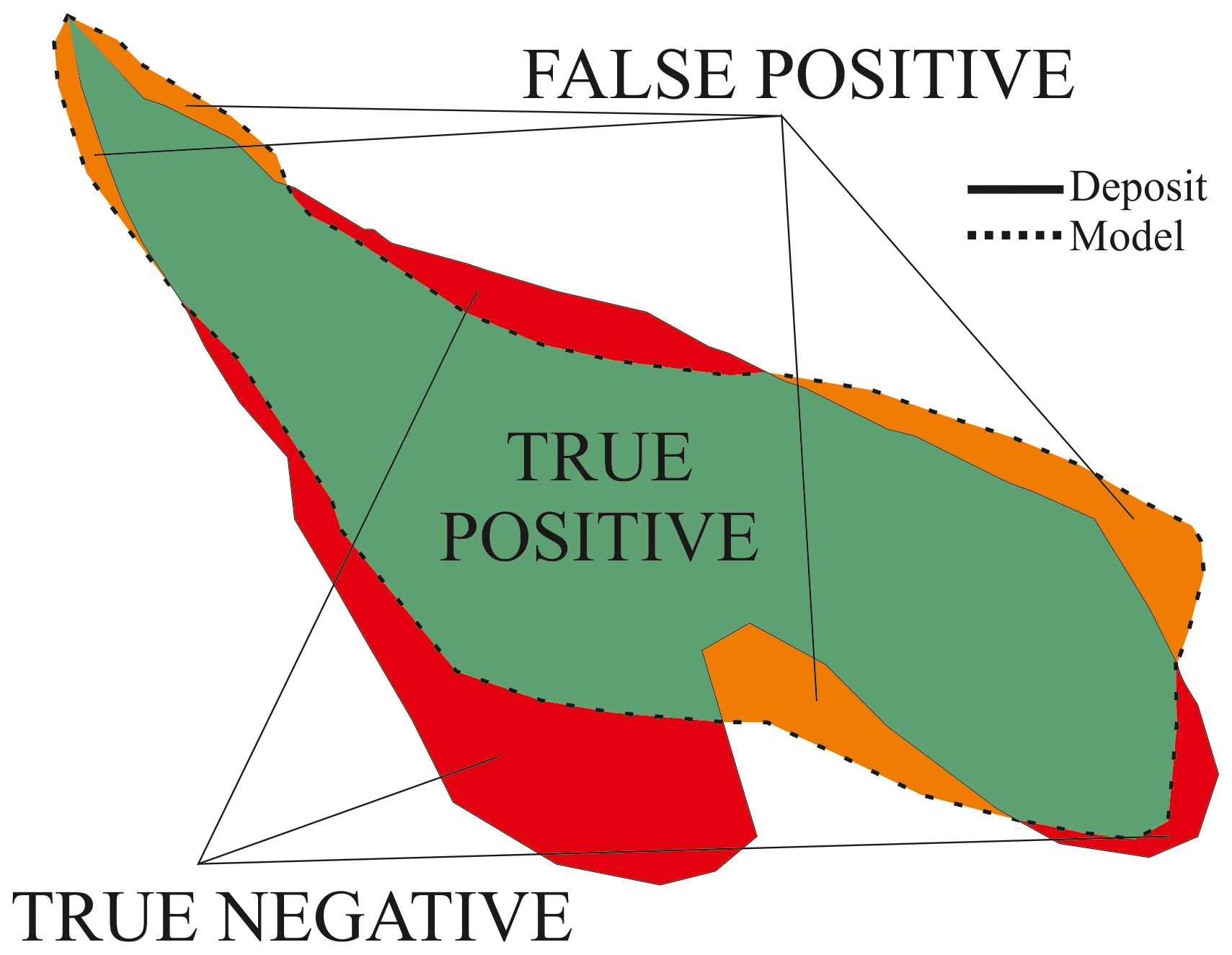
Figure 5 Sketch representing the three areas used for the validation procedure (the model output outline is drawn as a dashed black line).

Finally, the comparison of volume fractions of different grain sizes has been performed using the mean value of, respectively, ash (<2 mm of diameter) or lapilli (>2 mm of diameter) for all the stratigraphic sections in Cioni et al. (2020) placed at similar distances from the vent area. Such values were compared with the corresponding volume fractions of the model at the same distances. In detail, we considered (i) 18 samples (in sectors N and S) for the EU3pf unit placed at distances from the vent area of 4 (5 N and 2 S), 6 (2 S), 7 (7 S) and 9 km (2 S) and (ii) 19 samples (in sectors NW and SE) for the EU4 unit placed at distances from the vent area of 4 (5 NW), 6 (4 SE), 9 (5 SE), 14 (4 SE) and 20 km (1 SE).

The scarcity of stratigraphic sections in the N sector (for the EU3pf unit) and the NW sector (for the EU4b/c unit) negatively affects the availability of comparisons with respect to volume fractions, which are limited to sections at 4 km of distance from the hypothetical vent area, most of which have been collected at the bottom of paleo-valleys. Moreover, for the EU3pf unit, even in the S sector the available samples are mostly concentrated in the area of Herculaneum (five samples).

4 Results

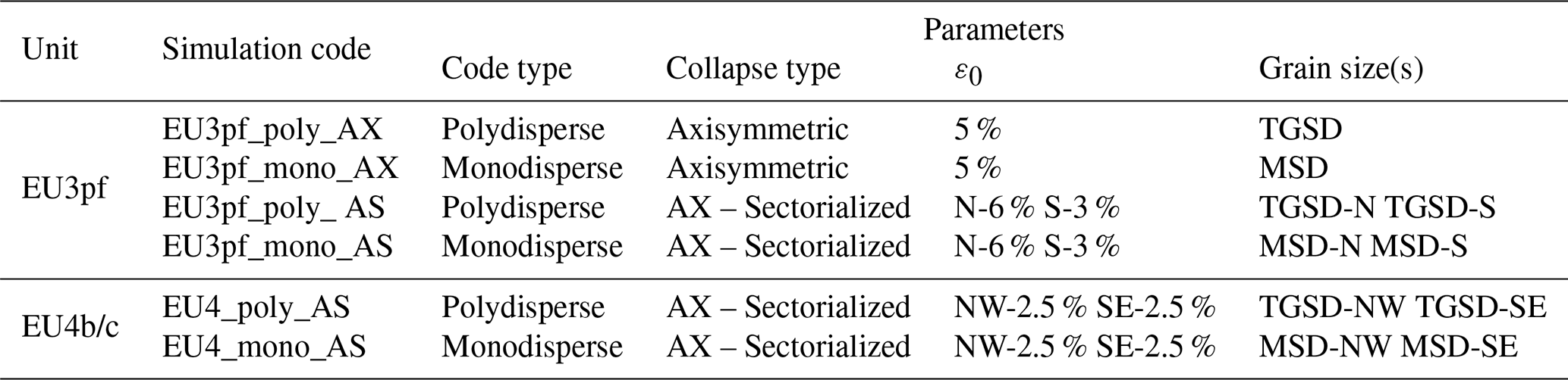
The results of six simulations (four for the EU3pf unit and two for the EU4b/c unit) are discussed here (see Table 4 for the main input parameters). These simulations are the result of an extensive investigation in which a wide range of different values of ε₀ have been tested, following a trial-and-error procedure aimed at reproducing more closely the thickness profile of the deposit. In particular, we performed several simulations varying ε₀ between 0.5 % and 6 % (for EU3pf) and between 0.1 % and 5 % (for EU4b/c). The values in Table 4 represent the optimal combinations.

Table 4 PyBox simulations for the EU3pf and EU4b/c units. Symbol key: AX – “axisymmetric”; AS – “axisymmetric–sectorialized”; ε₀ – “volumetric fraction of solid particles”.

We adopted a simplified version of the paleo-topography prior to the 79 CE eruption starting from the 10 m resolution digital elevation model of Tarquini et al. (2007) and from the reconstruction given in Cioni et al. (1999) and Santacroce et al. (2003) (Fig. 8). The modern Gran Cono edifice and part of the caldera morphology have been replaced with a flat area, and a simplified reconstruction of the southern part of the Mount Somma scarp has been inserted. However, simulations performed using the unmodified digital elevation model (DEM) did not produce major differences.

In the EU3pf case study, we performed both axisymmetric simulations over a round angle (given the quasi-circular shape of the deposit) and also axisymmetric–sectorialized simulations to investigate possible sheltering effects of the Mount Somma scarp (Fig. 2a). We modelled two distinct column collapses, one to the north and the other to the south, each of which has a collapsed volume corresponding to the actual deposit volume in that sector. In the EU4b/c case study, we performed only axisymmetric–sectorialized simulations, to reproduce more closely the dynamics of the related collapse, as indicated by the different dispersal in the NW and SE sectors of the PDC deposit (in particular, two distinct collapses for the same simulation, one to the NW and the other to the south-east).

In summary we provide (a) the thickness comparison between deposit and modelled results (Fig. 6) and between simulations done with a different initial volumetric fraction of solid particles (ε₀ – Fig. 7); (b) the inundation areas, including the quantitative matching of simulations and actual deposit (Fig. 8 and Table 5); and (c) the grain size distribution comparison, between deposit and modelled values, i.e. the volume fractions of ash vs. lapilli (Fig. 9) and of all the grain size classes (Fig. 10).

5 Analysis and discussion

5.1 General considerations

Testing PyBox with respect to field data is aimed at two main objectives: (i) quantifying the degree of reproduction of the real PDC deposit of Plinian eruptions in terms of thickness, inundation area and grain size and (ii) evaluating the reliability of the code when considering different assumptions, i.e. polydisperse vs. monodisperse situations, and 360^∘ axisymmetric conditions vs. dividing circular sectors. Before commenting on our results, two main general considerations, common to both EU3pf and EU4b/c, deserve a special discussion.

5.1.1 Run-out truncation and non-deposited material

PyBox produces the map of the inundated area (Neri et al., 2015; Bevilacqua, 2016), by truncating the run-out wherever the kinetic energy of the flow is lower than the potential energy associated with a topographic obstacle (Sect. 2.1 and Appendix A). In this way, however, the material that lies beyond the truncation is neither redistributed nor considered any more. However, depending on the topography in our case study, this amount of material is not extremely high. For instance, EU4_poly_AS (Table 4), in its SE part, has several truncations due to the intersection of the decay function of kinetic energy with several topographic barriers, i.e. the Apennines to the ENE and the Sorrentina Peninsula to the south-east (Figs. 2 and 7). For the whole SE part of the deposit, the topographic barriers are located between 11.85 and 19.25 km from vent area, with a mean value of 15 km. If we truncate PyBox deposit corresponding to these three limits, the non-deposited volume is between 3.46×10⁶ m³ (cut at 19.25 km) and 2.3×10⁷ m³ (cut at 11.85 km), with a mean value of 1.27×10⁷ m³ (cut at 15 km). Considering that the volume collapsed to the south-east is 1.5×10⁸ m³, the non-deposited volume therefore corresponds to a value between 2 % and 15 %, with a mean of 8 %. The amount of volume effectively “lost” is relatively small, also considering that the total volume of the collapsing mixture is inclusive of the EU4c unit (co-ignimbritic part). However, further development of the code might consider a strategy to redistribute this non-deposited material (e.g. Aravena et al., 2020).

5.1.2 Initial volumetric fraction of solid particles

The value of the initial volumetric fraction of solid particles (ε₀) in the PDC represents one of the most uncertain parameters, for which few constraints exist. Recently, Valentine (2020) performed several multiphase simulations using mono- or bi-disperse distributions to investigate the initiation of PDCs from collapsing mixtures and to derive criteria to determine when either a depth-averaged model or a box model are best suited to be employed for hazard modelling purposes. The author concluded that, among other factors (e.g. impact speed or relative proportion of fine to coarse particles), a volumetric concentration of particles of around 1 % (slightly lower than those used in this paper), and where ≈50 % or more of the particles are relatively coarse, is generally capable of producing a dense underflow and a dilute, faster overriding flow. For such cases, Valentine (2020) suggests that a depth-averaged granular flow model approximates such dense underflows well and could be reasonably used for hazard assessment purposes. For the units studied here, the sedimentological features show that there is clear evidence of the formation of a dense underflow in, respectively, the north part of the Somma–Vesuvius volcano (EU3pf unit; Gurioli et al., 1999), corresponding to the urban settlements of Herculaneum and Pompeii (EU4 unit; Cioni et al., 1999; Gurioli et al., 2002). However, we think the employment of a box model is justified for at least the unit EU4b/c, which can be regarded as intermediate between a dilute, turbulent and a granular concentrated current, in the sense of Branney and Kokelaar (2002), but closer to the dilute endmember type. In this view, the box model can be effectively employed to describe the overriding dilute part units similar to the EU4, following a two-layer approach (Kelfoun, 2017; Valentine, 2020).

For the box model used here, it should be kept in mind that the variation in the ε₀ value might have an important effect on the simulated deposit thicknesses, as seen in Fig. 7. In both units, in fact, the model results for thickness at the beginning of the simulated area (i.e. 3 km from vent area) vary from ca. 1 to ca. 2 m (for EU3pf) or from ca. 1.2 to ca. 3.6 m (for EU4b/c) if ε₀ is varied, respectively, from 1.5 % to 6 % and from 0.5 % to 5 %.

5.2 Thickness comparison

The first parameter that we compare between the deposit and the modelled results is the thickness variation with the distance to the source, an approach already adopted, for instance, by Dade and Huppert (1996). Our comparison focuses on the average thickness calculated over concentric circles drawn with a 100 m step of distance. However, the thickness variation in the deposit in different radial directions describes two different situations for the EU3pf and EU4b/c units and deserves a brief discussion, detailed in Appendix B.

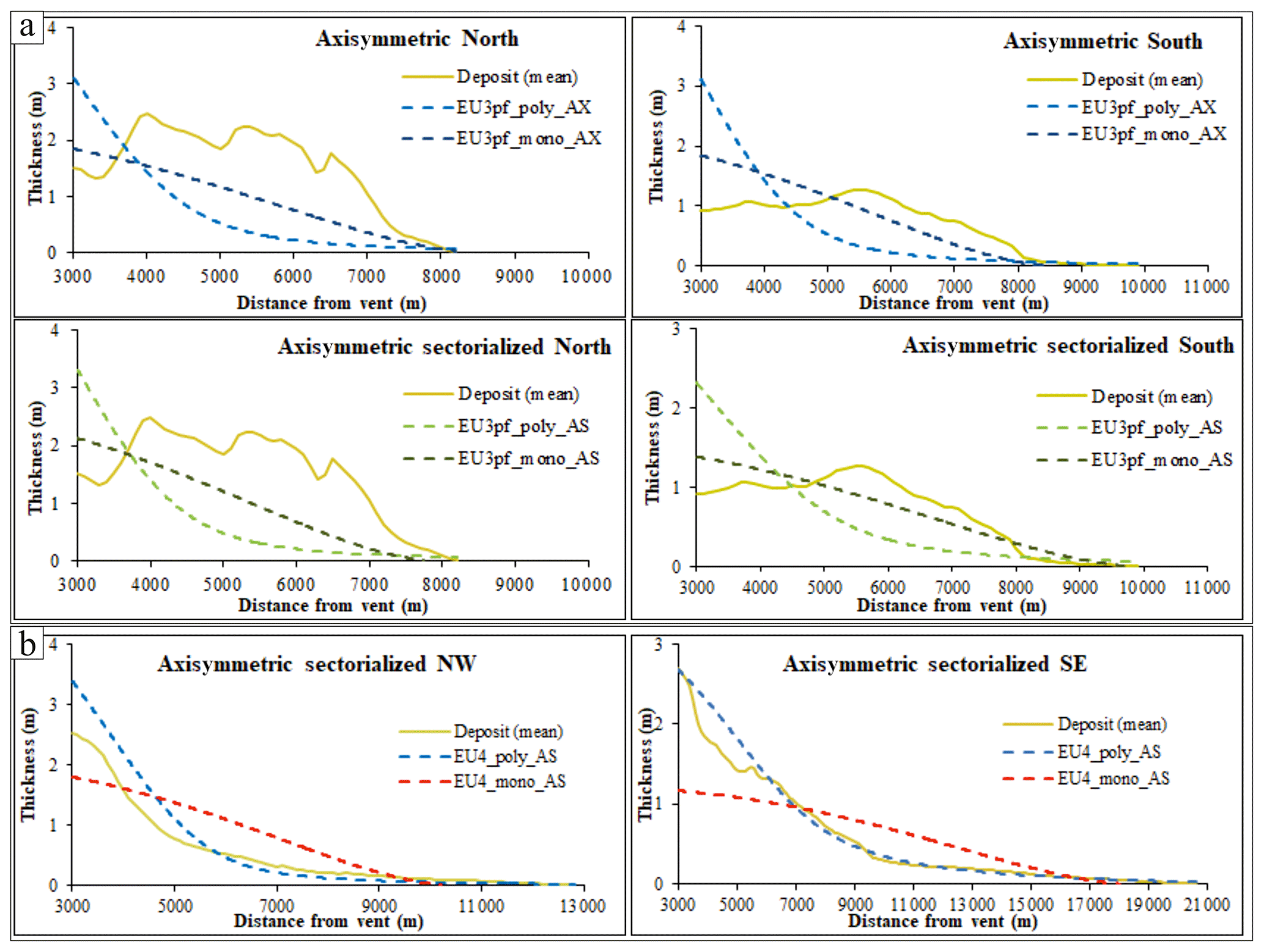
Figure 6 Mean thickness comparison between the simulations (dashed lines) and the actual deposit (solid line) of (a) EU3pf and (b) EU4b/c units. Different boxes concern different circular sectors.

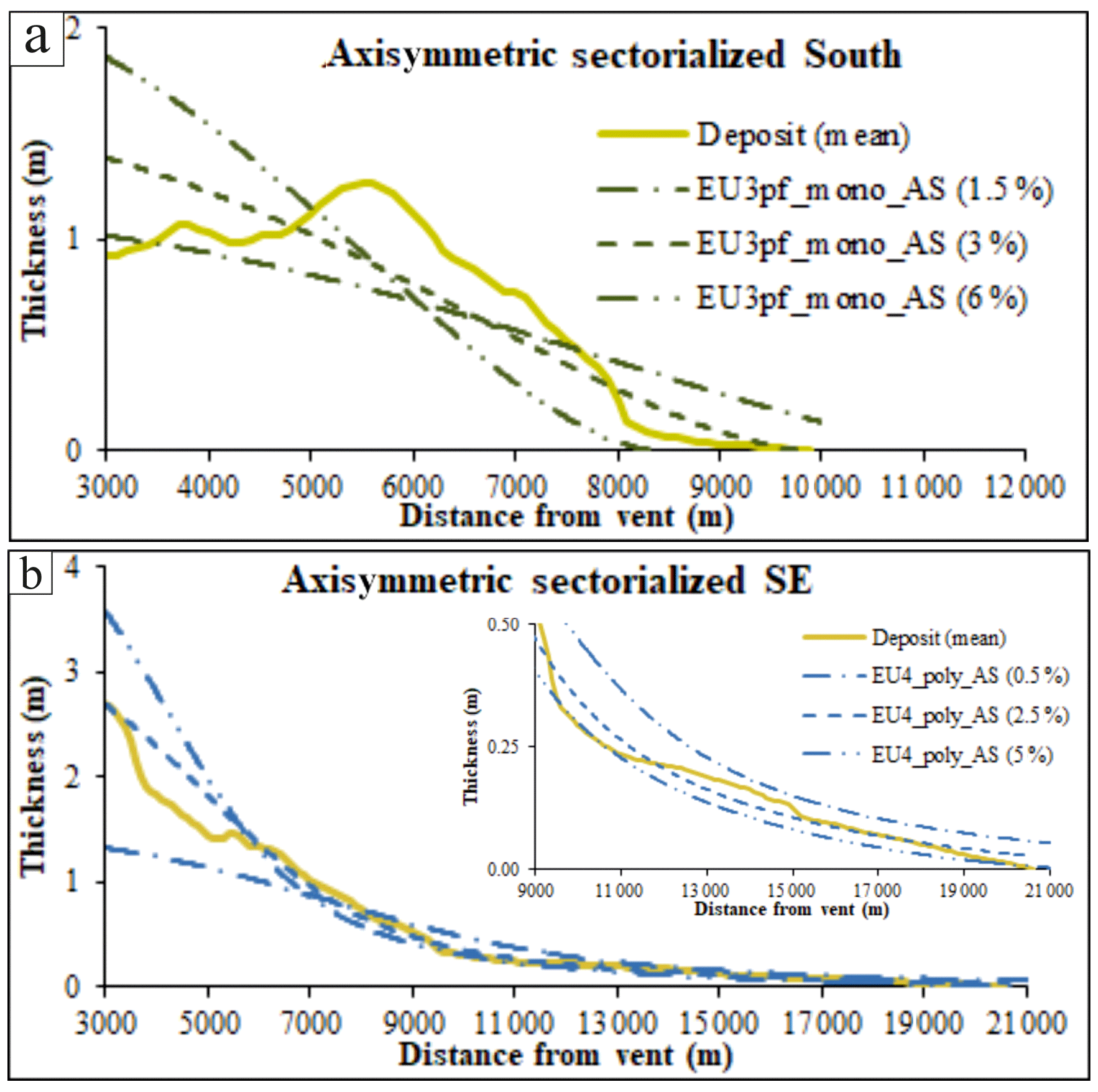
Figure 7 Comparison between simulations (dashed lines) assuming different initial volumetric fractions of solid particles (ε₀) and the actual deposit (solid line) of the (a) EU3pf unit S and (b) EU4b/c unit SE. In (b), the inset is a magnification of the thicknesses more than 9 km from the vent.

The average thickness of the EU3pf deposit mean profile initially shows an increasing trend (between 3 to 4 km to the north and between 3 to 6 km to the south – Fig. 6a) followed by a slow, constant decrease. This situation could highlight a lower capability of the current to deposit in more proximal areas, allowing the mass to be redistributed toward more distal sections. This could also be motivated by a spatial variation in the PDC flux regime, which was more turbulent in proximal areas than in distal ones, as also testified by the abundance of lithofacies typical of dilute and turbulent PDCs (//LT to xsLT; see Fig. 2b and Gurioli et al., 1999). Instead, the spatial homogeneity of lithofacies for the EU4b/c unit (Cioni et al., 1992) suggests a higher uniformity of its parent PDC. Moreover, the trend of the mean deposit thickness profile has a steep and rapid decrease in thickness of up to 5–6 km, followed (after a break in slope) by a “tail” with an increasing gentler decrease in thickness. This peculiar trend is in agreement with the lithofacies association in the unit EU4b/c (Cioni et al., 1992), which indicates a progressive dilution of the current through time and a progressive aggradation of the deposit. This trend might moreover be put in relation to the non-exponential decay of sedimentation with distance, described by Andrews and Manga (2012) for dilute PDCs associated with the formation of co-ignimbritic plumes.

That said, the degree of matching between the modelled and the real thickness of the EU3pf unit is less accurate than in the EU4b/c case study. However, the mean thickness profile of the actual deposit is roughly parallel with the model, in some parts. Under polydisperse conditions, PyBox does not improve its performance in replicating the thickness profile of EU3pf. The difficulties of PyBox in reproducing the thickness average profile reflects the likely dominant role of the density stratification and granular transport in the deposition process in areas of complex topography (Gurioli, 1999; Cioni et al., 2020). To the north there was in fact an extremely rough topography, similar to the present one, where the interaction of the PDC with the surface produced largely variable lithofacies. To the south, by contrast, there was a gentler topography, with a topographic high on which the town of Pompeii (see Fig. 2a) was built. This latter aspect is also evident from Vogel and Märker (2010), who reconstructed the pre-79 CE paleo-topography of the plain to the south-east of the SV edifice. From this work, it is possible to appreciate how the modelled depth of the pre-79 CE surface is 0–1 m lower with respect to the present surface corresponding to the present town of Pompeii and the ancient Pompeii excavations (due to the presence of piles of tephra fallout deposits up to 2 m thick), while it is up to 6–7 m deeper to the north-west of these sites.

The thickness comparison of the EU4b/c unit, by contrast, suggests that this unit was likely deposited under inertial flow conditions, dominated by turbulent transport. The SE tail part of the deposit is particularly very well reproduced by the polydisperse simulations, where the simulated profile is almost coincident with the deposit profile (Fig. 6b – right). Conversely, to the north-west the modelled thickness in the initial part overestimates the real deposit a bit (Fig. 6b). The polydisperse simulations (blue dashed lines in Fig. 6b) are much closer to the measured trend of the mean thickness profile than under the monodisperse conditions (i.e. MSD), demonstrating the key role of the grain size distribution in gas-particle turbulent transport.

5.3 Comparison of inundated areas

The areal overlapping between the model output area and the actual deposit (true positive – TP) is discussed together with the quantification of model overestimation (false positive – FP) and underestimation (true negative – TN). In Table 5 we also provided the TP, FP and TN estimates for the 5th and 95th percentiles of the maximum run-out lines (MRLs), i.e. a measure of the spatial uncertainty affecting the actual deposit. We remark that the TN instances could be interesting from a hazard point of view because they actually represent the underestimation of the model: a conservative approach is therefore to use the lowest value of the TN instances as a threshold to evaluate the reliability of a model.

Table 5 True positive (TP), false positive (FP) and true negative (TN) instances of the simulations in Fig. 8.

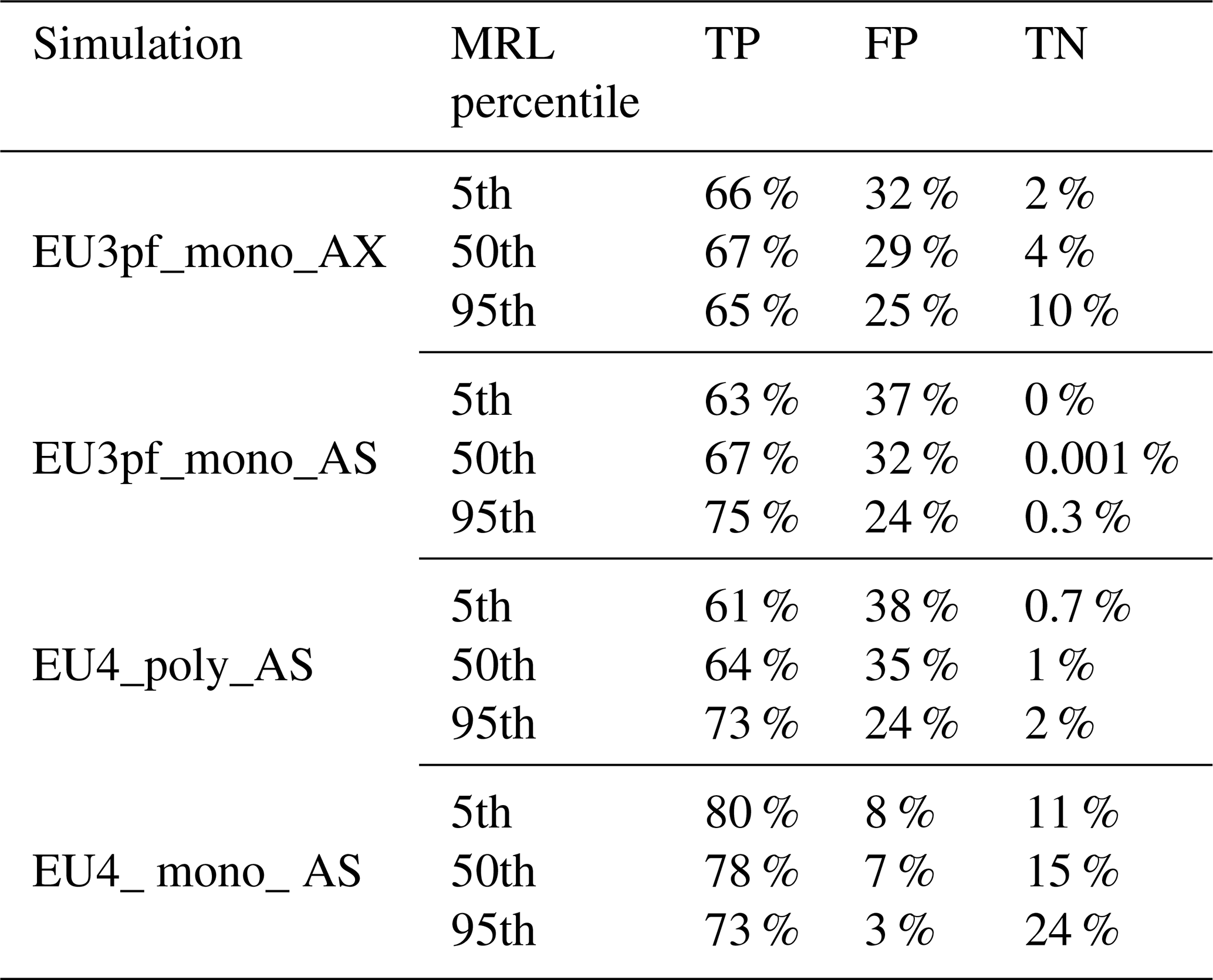
As said above, the polydisperse simulations of the EU3pf unit poorly fit with the deposit thickness, and the inundated area is significantly larger than the deposit area. Thus, they are not included in the quantitative estimation of area match or mismatch. For instance, while the maximum run-outs of the deposit are on the order of 8–10 km, the maximum run-out given by the model (in the absence of topography) is ca. 13–15 km. The monodisperse simulations perform better, in this sense, and maximum run-outs are slightly different (ca. 7–10 km) from the real ones: for this reason, only the monodisperse simulations for the EU3pf case have been considered in Fig. 8 and Table 5. More precisely, the axisymmetric EU3pf_mono_AX and the sectorialized EU3pf_mono_AS share a similar degree of TP instances (between 63 % and 75 % – Table 5) but have opposite properties for what concerns overestimation or underestimation. EU3pf_mono_AX has in fact a higher tendency to underestimate deposits (FP<TN – Table 5), while EU3pf_mono_AS tends to overestimate the actual deposit (FP>TN – Table 5).

For what concerns the EU4b/c simulations (Fig. 8), we report the quantitative matching of both the simulations under polydisperse and monodisperse conditions. The most striking feature that could be seen from Fig. 8 is that, while to the south-east a good match is obtained, to the north-west the polydisperse simulation overestimates the inundation area. Conversely, the monodisperse simulation is more balanced between NW and SE. This could be related, for the SE part, to the surrounding morphology of the Sorrentina Peninsula and the Apennines, which act as a natural barrier and, for the NW sector, to the absence of morphological constraints especially to the north. The results presented in Fig. 8 and Table 5 show that the TP values for the simulation EU4_poly_AS are in the interval 61 %–73 %, while TN values range from 0.7 % and 2 % and FP values range from 24 % and 38 %. Thus, while the degree of overlap between model and deposit is at an acceptable value and the percentage of model underestimation is below 2 %, the model tends to appreciably overestimate the median outline of the deposit. By contrast, the simulation EU4_mono_AS shows the highest TP values (73 %–80 %) and the lowest FP (3 %–8 %). Despite these better performances, it should be kept in mind how the thickness profile is less accurate under monodisperse conditions.

Beyond 14 km (ca. 2–3 km beyond the deposit MRL₉₅) the thickness provided by the model under polydisperse conditions is <1 mm (see Fig. 8c). Thin deposits might possibly be affected by erosion, and the actual deposit in the NW sector might in fact resemble the PyBox results. We also note that the MRLs defined by Cioni et al. (2020) have been defined up to the 95th percentile, meaning that there is still a 5 % chance that the actual MRL could be placed further away from the source. This is very significant in the NW part of the EU4b/c deposit, where no or very few outcrops can be found beyond 5–6 km from vent area.

5.4 Grain size comparison

Finally, we consider the volume fraction of the grain sizes of the actual deposits versus those derived from PyBox. We present the results in two different ways. Firstly, we provide a general overview of what the relative proportions of ash or lapilli are with distance to the source (Fig. 9), and then we provide more complete volumetric grain size comparisons for each Φ unit (Fig. 10). This comparison is one of the most uncertain because of some inherent epistemic uncertainties in the data: (i) the complete lack of ultra-proximal sites possibly enriched in coarse-grained particles that influenced the calculated TGSD; (ii) the fact that the sections used for TGSD calculation and data comparison are (for both units) located mainly along the aprons of the volcano, in many cases corresponding to the lower parts of valleys or paleo-valleys. This could have led to have an underrepresentation of the finer-grained deposits located in high or paleo-high morphological locations.

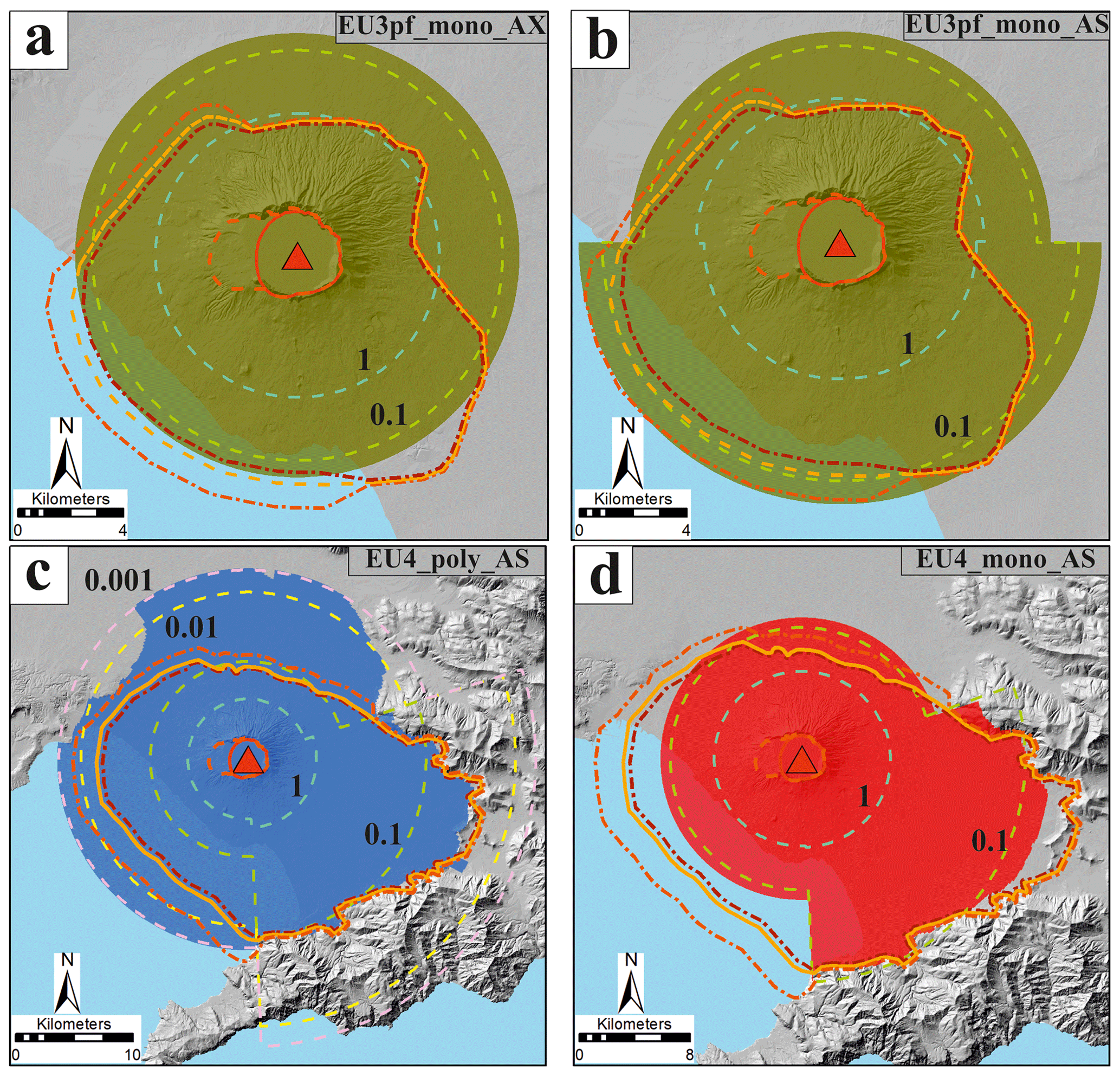
Figure 8 Inundation area of the simulations of the EU3pf (a, b) and EU4b/c (c, d) units. The dashed lines represent the theoretical isopachs (in m) of the simulated deposit. Vent location (red triangle), vent uncertainty area (red line) and SV caldera (orange dashed line) as in Tadini et al. (2017). MRLs as in Fig. 3. The DEM used in the simulations and as a background derives from Tarquini et al. (2007) according to the modifications explained in Sect. 4.

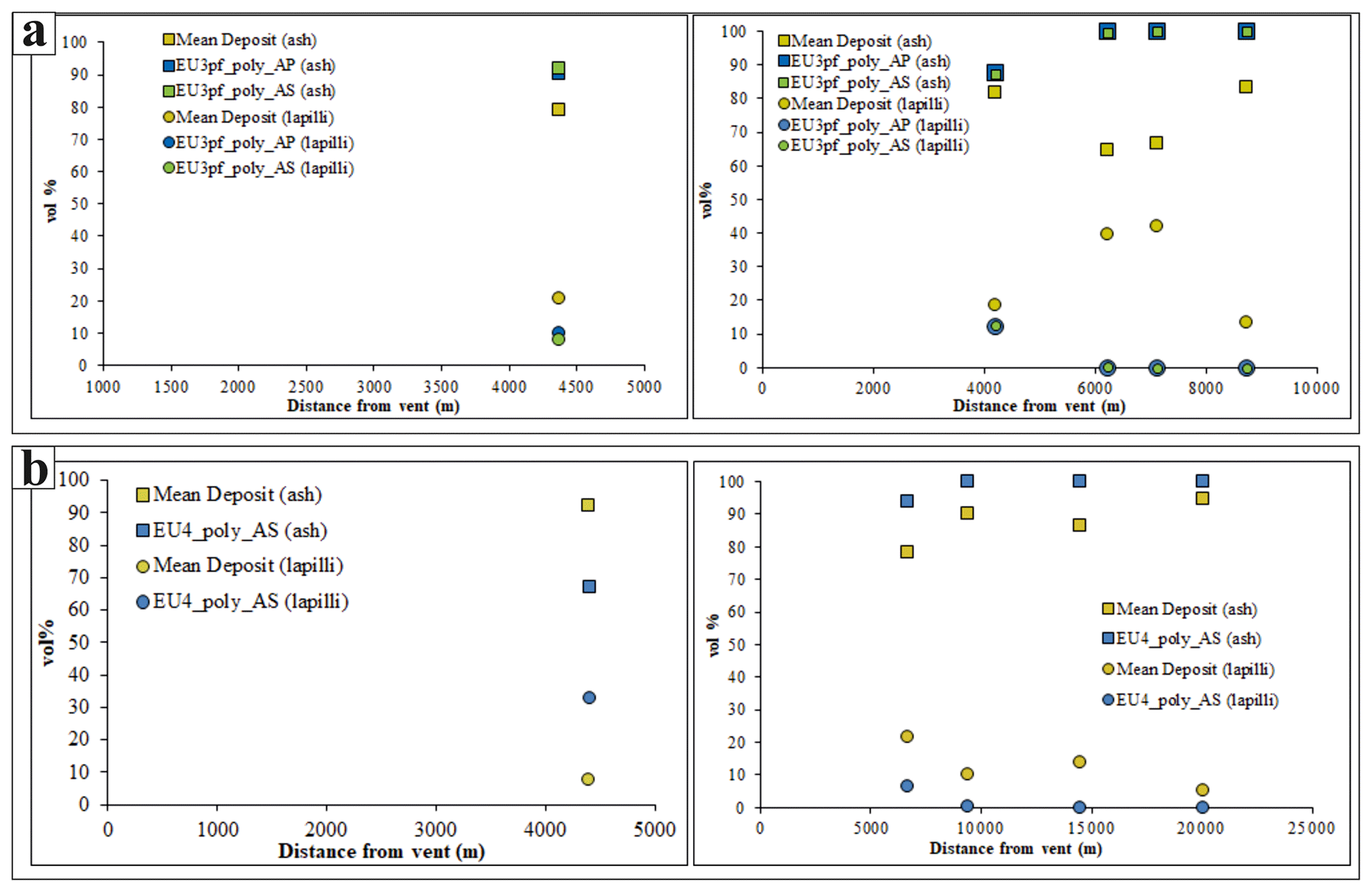
Figure 9 Volumetric content of ash or lapilli of model or deposit with distance to the source of the units (a) EU3pf N/S (left and right, respectively) and (b) EU4b/c NW/SE (left and right, respectively).

The data presented in Fig. 9 confirm the differences between EU3pf and EU4b/c. EU3pf (Fig. 9a) shows that the simulated and real volumetric contents of ash or lapilli are similar only up to 4 km (both to the north and to the south). Then, the relative proportions of ash or lapilli in the simulations indicate that, after 6 km, the simulated grain sizes are made almost entirely (>90 %) by ash, with a sensitive difference with respect to field data (only to the south, as to the north there are no available measurements). The most extreme situation could be seen at 9 km, where the modelled grain sizes are composed for >80 % in volume by the two finest ones (4–5 Φ), while deposit data indicate a more equal distribution of grain sizes. In Fig. 10a we observe that at 4 km (both N and S) the grain size distributions are similar between the actual deposit and the model, although there is a shift of ca. 2 Φ toward the finer grain sizes in the modelled data.

For the EU4b/c unit, we observe that the general proportions between ash and lapilli (Fig. 9b) are more similar between the model and the deposit (especially at 4 km from the vent area to the north). However, in Fig. 10b we see that at 4 km to the north, the situation is the opposite of EU3pf, since the modelled grain size is richer in coarse particles than the actual deposit. Such difference might be motivated by the above-mentioned roughness of the topography, which might favour the deposition of coarser particles at locations <4 km. In the SE sector the differences between modelled and observed grain sizes are lower at 6 and 9 km distance to the source, while they are greater at 14 and 20 km, where the two finest modelled grain sizes account for >80 % of the volume.

6 Conclusions

We have evaluated the suitability of the box-model approach implemented in the PyBox code to reproduce the deposits of EU3pf and EU4b/c, two well-studied PDC units from different phases of the 79 CE Pompeii eruption of Somma–Vesuvius (Italy). The total volume, the TGSD, the grain densities and the temperature obtained from the field data are used as the main inputs of PyBox. The model produces several outputs that can be directly compared with the inundation areas and radially averaged PDC deposit features, namely the unit thickness profile and the grain size distribution as a function of the radial distance to the source. We have performed simulations either under polydisperse or monodisperse conditions, given by, respectively, the total grain size distribution and the mean Sauter diameter of the deposit. We have tested axisymmetric collapses either as round angle or divided into two circular sectors. The initial volumetric fraction ε₀ of the solid particles over the gas is the main tuning parameter (given its uncertainty) that is explored to fit the outputs with the field data. In this study, we obtained the best fit of deposit data with a plausible initial volume concentration of solid particles from 3 % to 6 % for EU3pf (depending on the circular sector) and of 2.5 % for EU4b/c. These concentrations optimize the reproduction of the thickness profile of the actual deposits.

Concerning the EU3pf unit, (1) the average thickness of the EU3pf deposit initially shows an increasing trend, from 3 to 4 km to the north and from 3 to 6 km to the south, followed by a slow, constant decrease. The simulated thickness poorly resembles the actual deposit, although the maximum values are comparable and the two profiles are roughly parallel, in some parts. Under polydisperse conditions, PyBox does not improve its performance in reproducing the thickness profile of EU3pf. (2) In the monodisperse simulations of EU3pf the maximum run-outs are slightly different from the real ones, but overall consistent. The round-angle and sectorialized simulations share a similar degree of TP instances (between 63 % and 75 %) but have opposite properties for what concerns overestimation or underestimation. The round-angle axisymmetric simulation underestimates the actual deposit (FP<TN), while the sectorialized simulation overestimates the actual deposit (FP>TN). (3) The simulated and real volumetric contents of ash or lapilli in EU3pf are similar only up to 4 km. Then, the relative proportions of ash or lapilli in the simulations indicate that the simulated grain sizes are made up almost entirely (>90 %) by ash, with a sensitive difference with respect to field data after 6 km. We observe that at 4 km the grain size distributions are similar between the actual deposit and the model, although there is a shift of ca. 2 Φ toward the finer grain sizes in the modelled data.

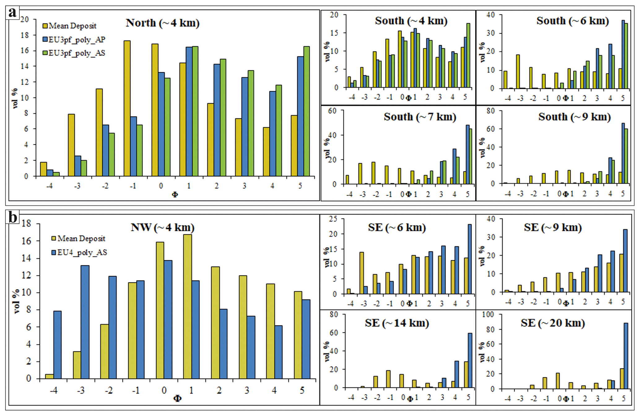
Figure 10 Comparison of volumetric grain sizes of the (a) EU3pf and (b) EU4b/c units. Different boxes concern different distances to the source.

Concerning instead the EU4b/c unit, (1) this unit has a steep and rapid decrease in thickness of up to 5–6 km, followed, after a break in slope, by a tail with a gentler decrease in thickness. The polydisperse box-model simulations are much closer to the measured trend of the mean thickness profile than under the monodisperse conditions. The SE thickness profile of the polydisperse simulation is almost coincident (within the uncertainty range) with the corresponding part of the deposit (specifically after 6 km and with a ca. 0.5 m overestimation between 3.5–6 km), while to the north-west the modelled thickness slightly overestimates the real deposit in the initial part (up to ca. 6 km). (2) In the simulations of EU4b/c, a good match of inundated area towards the south-east is obtained. Towards the north-west the polydisperse simulation sensibly overestimates the inundation area. By contrast, the simulation under monodisperse conditions shows the highest TP values (73 %–80 %) and the lowest FPs (3 %–8 %). However, the thickness profile is less accurate under monodisperse conditions. Moreover, thin deposits in the NW sector might possibly be affected by erosion, and the actual deposit in the NW sector might in fact resemble the PyBox results obtained under polydisperse conditions. (3) The general proportions between ash and lapilli in EU4b/c are similar in the model and the deposit. However, at 4 km to the north, the situation is the opposite of EU3pf, since the modelled grain size is richer in coarse particles than the actual deposit. In the SE sector the differences between modelled and observed grain sizes are lower at 6 and 9 km distance to the source, while they are greater at 14 and 20 km, where the two finest modelled grain sizes account for >80 % of the volume. (4) In the SE sector, because of model run-out truncation, we evaluated an average non-deposited volume of 1.27×10⁷ m³ (cut at 15 km). Considering that the volume collapsed to the south-east is 1.5×10⁸ m³, the average non-deposited volume therefore corresponds to a value of 8 %. Thus, the amount of volume effectively lost with the PyBox approach is relatively small, also considering that the total volume of the collapsing mixture is inclusive of the co-ignimbritic part.

Pyroclastic density currents generated by Plinian eruptions span a wide range of characters and can display very different behaviour and interaction with the topography. During the 79 CE eruption of Somma–Vesuvius, two PDC units, despite both being emplaced after column collapses, display significantly different sedimentological features and should likely be better described by different models. The study findings indicate that the box model, which is suited to describe turbulent particle-laden inertial gravity currents, describes the EU4b/c PDC unit well but is not able to accurately catch some of the main features of the EU3pf unit. This is probably due to its strongly density-stratified character, which made the interaction with the topography of the basal concentrated part of the flow a controlling factor in the deposition process. Results again highlight the key role of the grain size distribution in the description of inertial PDCs: while the final run-out is mostly controlled by the finest portion of the distribution, the total grain size distribution strongly affects the thickness profile (e.g. Fig. 6b), and it is an essential ingredient for proper modelling of the PDC dynamics.

Our study also highlights the importance of assuming axisymmetric or sectorial propagation of the PDCs. This is an additional source of uncertainty in Plinian (VEI 5) eruptions, in which PDCs are often generated by asymmetric column collapse. In the reproduction of a specific deposit unit, considerations about different propagation along specific sectors should be taken into account.

In conclusion, while the box-model approach is certainly suited to describe large-volume (VEI>6) low-aspect-ratio ignimbrites, some care should be taken when it is applied to smaller PDC-forming eruptions on stratovolcanoes, since the topographic effects due to flow stratification, not considered by the model, might be dominantly important. However, we believe that the approach, despite its simplifying assumptions, represents the behaviour of PDCs emplaced under turbulent conditions well, in situations where the effects of the topography on the transport system are negligible, and it can be used to assess the hazards associated with this type of flow. The box model is a valuable tool for PDC modelling in situations where topography is relatively simple and smooth (such as the area south of Somma–Vesuvius). On the other hand, caution must be exercised in cases of complex topography, where the effects of density stratification within the currents, which is not modelled with the box-model approach, plays a strong role in current behaviour and deposition.

Appendix A: Numerical solution of the box-model equations in the PyBox code

The set of equations of PyBox is numerically integrated by using a 2D embedded Runge–Kutta 3(2) method, following the scheme proposed in Bogacki and Shampine (1989). With respect to the more widely used Runge–Kutta 4(5), this approach is preferred because it succeeds in preserving the monotonicity of the settling solid fractions. In particular, we solve the box-model equations with the function scipy.integrate.solve_IVP, available in Python-3.x. We specifically considered the case when the computed solid fractions numerically fall below zero. We avoided this situation by interrupting the integration process whenever one or more solid fractions became lower than zero or extremely small. We restart the process with a new initial value obtained by setting such fractions to zero. The solver is also interrupted when the reduced gravity g^′ falls below zero, regardless of the values of the solid fractions. The asymptotic, stationary settling velocities of the particle classes are calculated by means of Newton's impact formula (Dellino et al., 2005; Dioguardi et al., 2018), where the gas-particle drag coefficient $C_{\mathrm{D}}^i$ is defined as a function of the relative gas-particle Reynolds number Re. The computation of settling velocities required an iterative procedure: in fact, Newton's impact formula was solved together with the relationship for the Reynolds number and the correlation between $C_{\mathrm{D}}^i$ and Re. In particular, we used the Schiller–Naumann correlation (Crowe et al., 2011), which accurately describes the drag force acting on a sphere with Re<1000, whereas, for Re>1000, we have set $C_{\mathrm{D}}^i=\mathrm{1}$, according to Woods and Bursik (1991).

Appendix B: Deposit thickness variations depending on the radial direction

Figure B1 describes the range of variability of the units' thickness collected in different locations. In EU3pf, a large variability – from 0 to 7.5 m in the N sector and from 0 to 5 m in the S sector – can be observed. This reflects how the EU3pf unit complexly interacted with the rugged topography that characterizes the aprons of the SV volcano. On the other side, for the EU4b/c unit the differences between deposit thicknesses from maximum and minimum are typically lower, i.e. from 0 to 4 m in the NW sector and from 0 to 5.5 m in the SE sector.

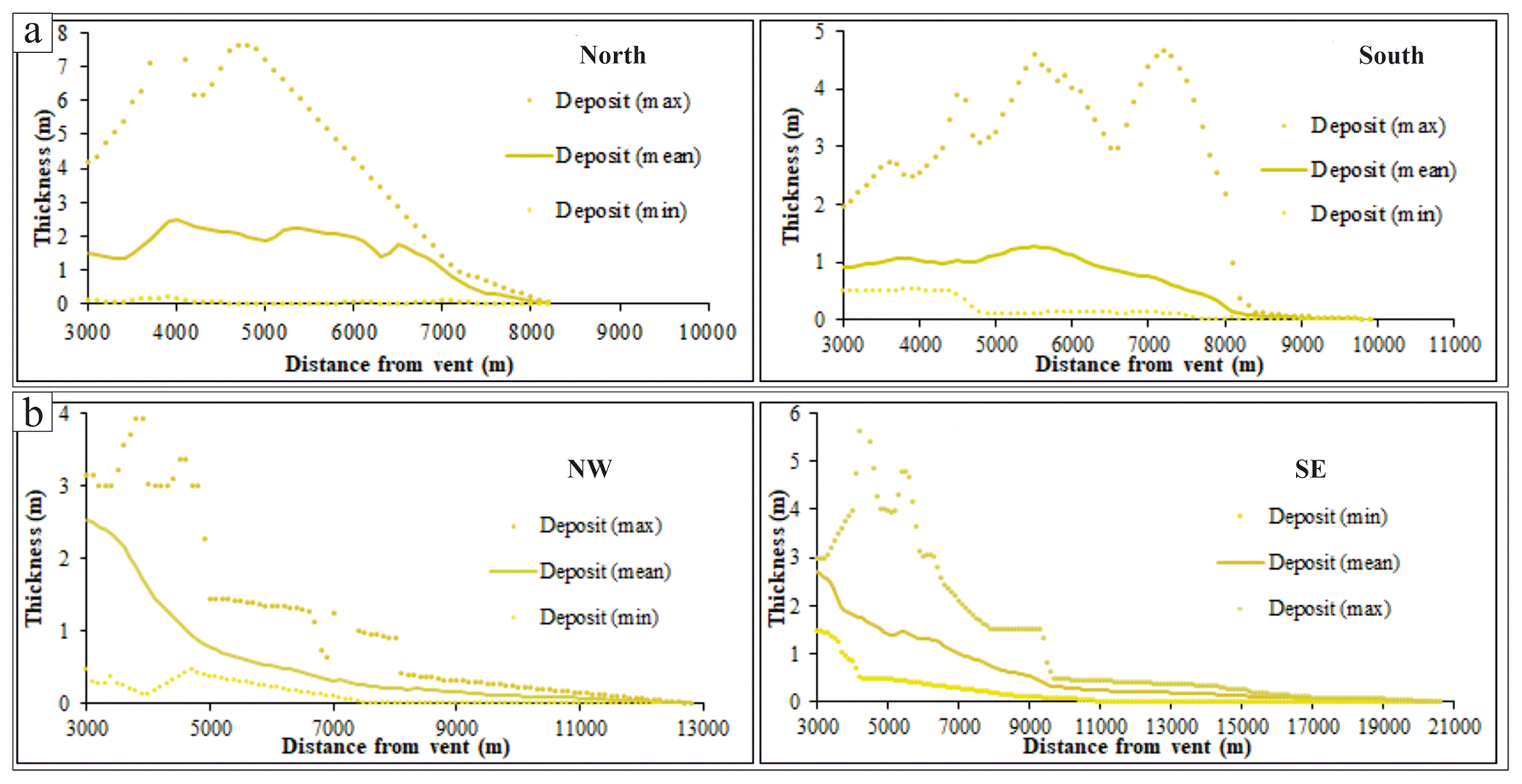
Figure B1 Deposit thickness for (a) EU3pf and (b) EU4b/c units. “Max”, “Mean” and “Min” refer to, respectively, the maximum, mean and minimum thicknesses measured along each circle described in Sect. 3.2.