the Creative Commons Attribution 4.0 License.
the Creative Commons Attribution 4.0 License.
 | 06 Jul 2021
Four-dimensional tracer flow reconstruction in fractured rock through borehole ground-penetrating radar (GPR) monitoring
Peter-Lasse Giertzuch
Joseph Doetsch
Alexis Shakas
Mohammadreza Jalali
Bernard Brixel
Hansruedi Maurer
Two borehole ground-penetrating radar (GPR) surveys were conducted during saline tracer injection experiments in fully saturated crystalline rock at the Grimsel Test Site in Switzerland. The saline tracer is characterized by an increased electrical conductivity in comparison to formation water. It was injected under steady-state flow conditions into the rock mass that features sub-millimeter fracture apertures. The GPR surveys were designed as time-lapse reflection GPR from separate boreholes and a time-lapse transmission survey between the two boreholes. The local increase in conductivity, introduced by the injected tracer, was captured by GPR in terms of reflectivity increase for the reflection surveys, and attenuation increase for the transmission survey. Data processing and difference imaging was used to extract the tracer signal in the reflection surveys, despite the presence of multiple static reflectors that could shadow the tracer reflection. The transmission survey was analyzed by a difference attenuation inversion scheme, targeting conductivity changes in the tomography plane. By combining the time-lapse difference reflection images, it was possible to reconstruct and visualize the tracer propagation in 3D. This was achieved by calculating the potential radially symmetric tracer reflection locations in each survey and determining their intersections, to delineate the possible tracer locations. Localization ambiguity imposed by the lack of a third borehole for a full triangulation was reduced by including the attenuation tomography results in the analysis. The resulting tracer flow reconstruction was found to be in good agreement with data from conductivity sensors in multiple observation locations in the experiment volume and gave a realistic visualization of the hydrological processes during the tracer experiments. Our methodology was demonstrated to be applicable for monitoring tracer flow and transport and characterizing flow paths related to geothermal reservoirs in crystalline rocks, but it can be transferred in a straightforward manner to other applications, such as radioactive repository monitoring or civil engineering projects.
- Article
(15889 KB) - Full-text XML
-
Supplement
(41914 KB) - BibTeX
- EndNote


Flow and transport processes in fractured rock have been a key focus of basic hydrogeological research and are relevant for numerous applications and research fields. These include risk assessment of contaminants (e.g., Andričević and Cvetković, 1996), nuclear waste disposal (Cvetkovic et al., 2004), and the exploitation of deep geothermal energy (DGE) (Brown et al., 2012). Virtually all fluid transport in granitic crystalline rock is carried by discrete permeable fractures that are connected within a fracture network. Field investigations in such complex subsurface environments are extremely challenging, as no complete direct observations of the fracture geometries and hydrological processes can be made. Conventional hydraulic and tracer tests only provide spatially discrete observations, such that flow and transport properties have to be interpolated or upscaled between observation points, or they have to be estimated with numerical simulations and simplifying assumptions. Therefore, the complex models needed for flow and transport in a discrete fracture network (DFN) can often only be weakly constrained by data. Additionally, the choice of a conceptual model introduces other simplifications, such as parallel plate approximations and radial flow assumptions (National Research Council, 1996). Therefore, generalized assumptions, based on local observations within the subsurface, may lead to significant uncertainties. For example, current models may encounter difficulties in estimating the effective surface area for heat exchange in natural fracture networks, which is highly relevant for DGE applications (de La Bernardie et al., 2019). Hawkins et al. (2017) reported significant differences in heat transport related to flow channeling within a fracture that was monitored with time-lapse ground-penetrating radar (GPR). Evidently, a better understanding of flow and transport in fracture networks outside of the lab scale is necessary (Amann et al., 2018), but the possibilities to locate and visualize flow paths within a fractured crystalline rock volume are limited.
Ground-penetrating radar (GPR) and GPR-responsive tracers are a possible option to monitor and visualize such processes. GPR makes use of electromagnetic waves in the MHz to GHz frequency range. As for any EM wave, the propagation in the subsurface is primarily dependent on the dielectric permittivity ε and the electrical conductivity σ of the host medium. While ε primarily affects the propagation velocity, σ primarily controls the wave attenuation. Depending on these subsurface parameters and the frequencies employed, GPR can be used for penetration depths extending from the centimeter range to hundreds of meters. The initial GPR pulse is reflected and/or transmitted at interfaces of contrasting electromagnetic parameters. The resulting signal can be recorded and estimations about the subsurface properties can be obtained (e.g., Jol, 2009).
GPR-responsive tracers that create a local contrast can be detected by comparing repeated GPR measurements during tracer and in situ water flow experiments. Such time-lapse GPR surveys are not as established as, for example, time-lapse electrical resistivity tomography (ERT) or time-lapse seismic imaging, but they can be useful in engineering and hydrology, as the electrical properties, sensed by GPR, can be affected by state variables of interest. Brewster and Annan (1994) were able to monitor dense nonaqueous phase liquid (DNAPL) spills, by exploiting their low relative dielectric permittivity (compared to the pore water). Also, the infiltration of water in unsaturated soil was successfully monitored with GPR (e.g., Trinks et al., 2001; Klenk et al., 2015). One key prerequisite of time-lapse GPR surveys is a high reproducibility and thus data consistency between the individual time steps. To this end, automated acquisition setups have been employed, such as that used by Mangel et al. (2020), who successfully demonstrated time-lapse reflection tomography to be capable of resolving water infiltration in the vadose zone. To resolve changes in time-lapse GPR images with higher robustness towards perturbations in the GPR traces that were unrelated to the monitored hydrological process, image similarity attributes were successfully applied (Allroggen and Tronicke, 2016; Allroggen et al., 2020).
For monitoring flow and transport processes in saturated media, electrical contrasts need to be introduced in the form of tracers. Salt water within a saturated environment with low formation-water conductivity introduces a local signal attenuation that was successfully detected in several cross-hole transmission GPR studies (Niva et al., 1988; Day-Lewis et al., 2003). Besides conducting transmission measurements, it is also possible to consider reflected GPR waves for detecting conductivity-changing tracers. The reflection from a thin conductive layer can be similar to a permittivity boundary, with a reflection coefficient and a phase shift dependent on the conductivity (Lázaro-Mancilla and Gómez-Treviño, 1996; Tsoflias and Becker, 2008).
If the tracer-induced change in the electromagnetic properties is small, as expected for small-aperture fracture networks or low tracer to formation-water contrast, elaborate difference approaches are needed to extract information. This has been demonstrated successfully for tracer tests in granite with reflection GPR (Dorn et al., 2011; Shakas et al., 2016). In theory, the difference between the reference and the monitoring data should contain only the tracer-induced changes, and static features from unchanged reflections should cancel out. However, for identifying subtle changes in the volume of interest, it is required to ensure a very high consistency and repeatability of the different data sets. Recently, an effective data processing procedure has been developed by Giertzuch et al. (2020a) that allowed for saline tracer signal extraction in a host rock with several reflectors and fracture apertures in the sub-millimeter range.
Unfortunately, there is no straightforward link between tracer-induced signal changes in GPR data and the governing material properties. Problems are caused by the azimuthal symmetry of GPR antennas, which makes it difficult to unambiguously identify the location of a reflector. Likewise, in the presence of a heterogeneous (with regards to GPR wave propagation) host rock, it can be difficult to relate travel times and amplitudes, obtained from transmission experiments, with the spatial distributions of the electrical permittivity and conductivity.
Some of these problems can be alleviated when the results of reflection and transmission surveys are combined. In this contribution, we present results from a field study, in which such a combined analysis allowed the 3D tracer flow path to be reconstructed. The approach is based on differencing schemes for both the reflection and transmission data. After describing the experimental setup, we present our processing workflows for the difference reflection imaging and the difference attenuation tomography. Finally, we outline how the resulting information can be combined to reconstruct the 4D tracer flow through the experiment volume.
2.1 Grimsel Test Site
The Grimsel Test Site (GTS) is an underground rock laboratory in Switzerland. It is located in a weakly fractured rock mass in the central Alps (Fig. 1). The GTS is operated by the National Cooperative for the Disposal of Radioactive Waste (Nagra) and has been used for a range of research projects (https://www.grimsel.com, last access: 15 June 2021). The experiments presented here were conducted in the scope of the In-situ Stimulation and Circulation (ISC) experiment (Doetsch et al., 2018; Amann et al., 2018; Krietsch et al., 2018). They were performed in the southern part of the GTS, located at a depth of about 480 m below the surface. The hydraulic heads indicate that the experiment volume and its fracture network are fluid-saturated. Figure 2 shows a geological model of the relevant part of the GTS, based on the work of Krietsch et al. (2018). The main features that influence fluid flow in the experimental volume include two brittle–ductile shear zones (S3, shown in green in Fig. 2). They intersect the AU tunnel (shown in cyan in Fig. 2) between four geophysical monitoring boreholes (GEO1 to GEO4), two of which (GEO1 and GEO3) were used for the GPR surveys. In total, 15 boreholes were drilled in the project volume to characterize the subsurface conditions. Besides the geophysical monitoring and the injection boreholes, these include three strain monitoring, three pressure monitoring, and three stress characterization boreholes (Doetsch et al., 2018). From this set of boreholes, only the ones relevant for this experiment are depicted in Fig. 2, namely the injection borehole (INJ2, green), the geophysical monitoring boreholes (GEO1 and GEO3, blue), and three pressure monitoring boreholes (PRP1-3, magenta). The PRP borehole intervals indicated in black contain permeable fractures and were permanently isolated. The tracer injection interval (INJ2.4), indicated by a red sphere at a borehole depth of 22.89–23.89 m, was isolated with straddle packers.
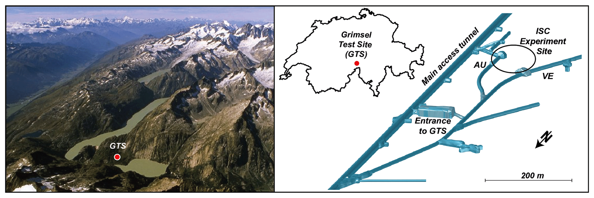
Figure 1GTS located in the central Alps in Switzerland. The ISC experiment was conducted in the southern part of the GTS, between the VE and the AU tunnels. Figure from Doetsch et al. (2017).
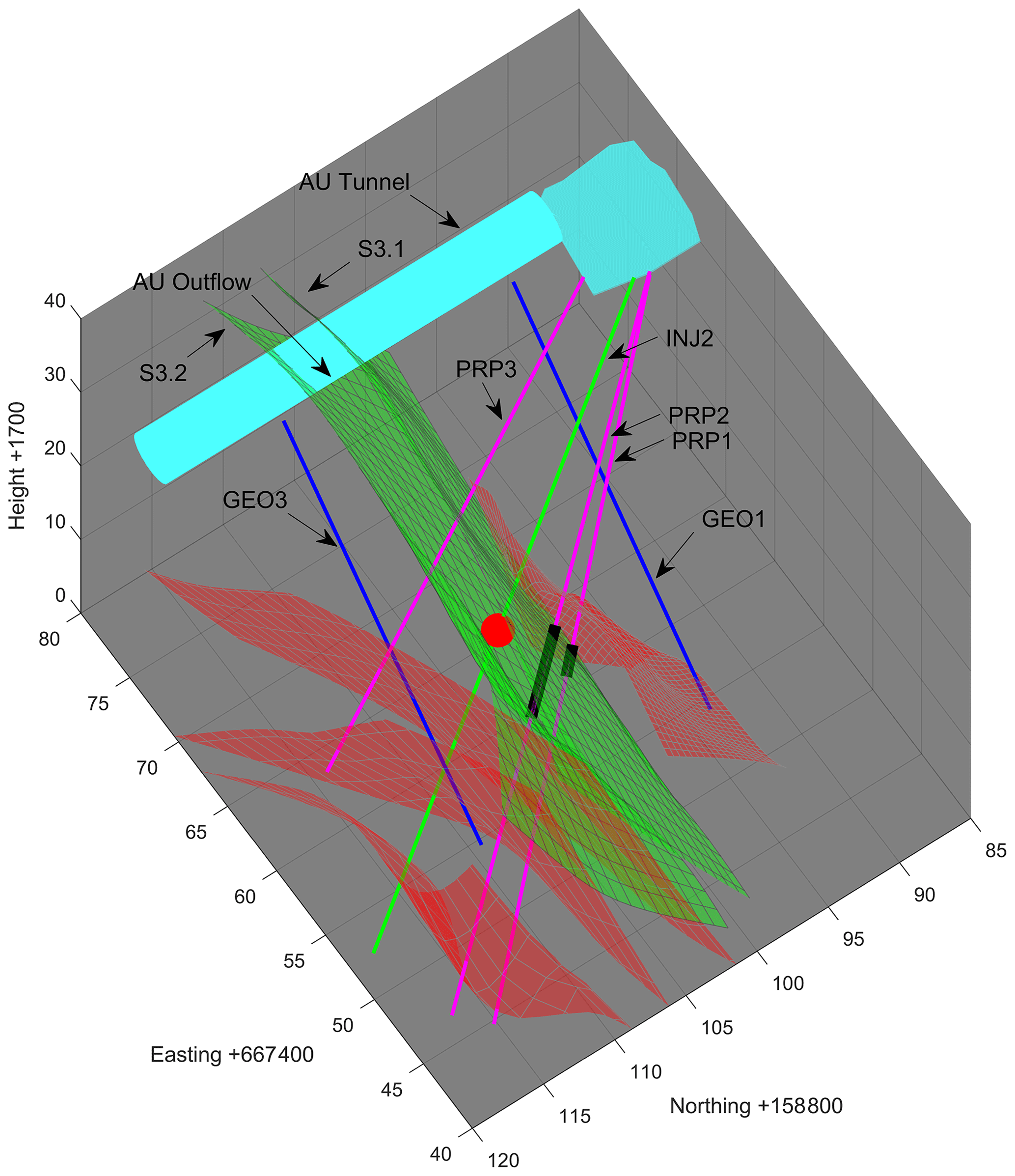
Figure 2Geological model of the experiment volume with relevant structures and boreholes. The S1 and S3 shear zones are shown in red and green, respectively. The GPR survey was performed in the blue GEO boreholes. The saline tracer injection point is indicated by a red sphere. Monitoring intervals in the PRP boreholes are indicated in black.
2.2 Grimsel ISC experiment
The controlled ISC experiment was carried out to investigate the seismo-hydromechanical processes during the creation of a geothermal reservoir. It included two stimulation phases, featuring hydraulic shearing and hydraulic fracturing that were conducted in February and May 2017, respectively (Amann et al., 2018). A comprehensive characterization of the relevant part of the GTS was crucial for a detailed understanding of the stimulation effects in the subsurface and a subsequent transfer of knowledge into reservoir creation. Therefore, in addition to the monitoring performed during the stimulations, pre- and post-stimulation characterizations were carried out with various geological, hydrogeological, and geophysical methods. A special emphasis was put on the fracture geometries and permeabilities, with the aim of a detailed flow field and fracture network reconstruction. Aside from GPR, as described by Giertzuch et al. (2020a), Doetsch et al. (2020), and in this study, extensive hydrologic testing was performed, tracer tests were conducted, and borehole logs were acquired, (e.g., Brixel et al., 2017; Jalali et al., 2018a; Krietsch et al., 2018; Kittilä et al., 2019; Brixel et al., 2020a, b; Kittilä et al., 2020a, b).
The fracture density in the host rock varies between 0 and 3 fractures per meter and can increase up to >20 fractures per meter between the S3 shear zones (Krietsch et al., 2018). Doetsch et al. (2020) found a decrease in seismic velocity between the S3 shear zones and were able to link this to a known increase in fracture density and permeability in this region (Krietsch et al., 2018; Brixel et al., 2020a). In the same study, surface GPR was used to identify the S1 and S3 shear zones but experienced low contrast for the S3 shear zones, due to the perpendicular orientation towards the survey tunnel. The GPR propagation velocity was found to be approximately 0.12 m/ns.
Fluid flow was shown to be primarily fault-controlled in well testing experiments by Brixel et al. (2020b), who found permeability to be strongly decreasing (from 10−13 to 10−21 m2) within 1 to 5 m from the fault cores. The S3 shear zones appear to have feature extension fractures that link the two S3 shear zones and create highly permeable cross-fault connections as shown in Brixel et al. (2020b). Additionally to the fault-controlled nature of the flow system, a drainage effect of the AU tunnel plays a key role in fluid flow at the ISC test site (Jalali et al., 2018b; Kittilä et al., 2020b). From dye and saline tracer tests in the INJ2.4 interval, connections towards PRP1.3, PRP2.2, and the AU tunnel have been found, with relatively fast breakthroughs in that order (Kittilä et al., 2020a, b; Giertzuch et al., 2020a; Jalali et al., 2019).
In a first-order estimate on hydraulic packer tests of single fractures, Brixel et al. (2020a) calculated equivalent hydraulic apertures to range from 2 to 130 µm, with a mean of 30 µm. However, this calculation relied on a parallel plate assumption with smooth fracture walls, yet locally the true fracture apertures may diverge significantly from this estimate.
2.3 GPR tracer experiments
Two GPR tracer experiments were conducted in November and December 2017. Each experiment relied on the same tracer and the same injection location, and they had a similar monitoring setup. A saline tracer with a conductivity of approximately 60 mS/cm was injected at a constant flow rate of approximately 2 L/min in the INJ2.4 interval, which is located in between the S3 shear zones, approximately 1.7 m below the GEO1–GEO3 plane (Fig. 2). The formation water showed a conductivity of around 0.08 mS/cm. Conductivity data loggers were connected to the AU outflow and to the intervals PRP1.3 and PRP2.2. Before and after tracer injection, formation water was injected continuously for several days at the same location and flow rate to ensure a steady flow state. For the first experiment, 100 L of saline tracer were injected over the course of 50 min, while for the second experiment the volume was doubled to 200 L, and the injection was performed over 100 min. The second experiment was performed during an ongoing heat injection experiment. While the hydraulic properties of the individual flow paths appeared to be affected by this (Kittilä et al., 2020a), the general flow path geometry can be assumed to have remained unchanged.
In general, the experiments were designed to be very similar to the experiment described and evaluated by Giertzuch et al. (2020a). The main differences included a larger injection interval and therefore higher injection rates, a higher tracer conductivity, the use of a salt-water tracer instead of a salt-water–ethanol tracer, a different GPR acquisition console, and slightly different GPR settings. The salt–water–ethanol tracer that was used by Shakas et al. (2017) and Giertzuch et al. (2020a) could compensate for the increased density of the saline tracer in comparison to the formation water, but in the experiments presented here, this mixture could not be used due to concerns about bacteria growth related to the ethanol. Since the results presented in Giertzuch et al. (2020a) showed comparable tracer appearances to the reflection results in this paper, the effect due to the density difference is assumed to be small. However, for comparisons with more conservative tracers, the density difference should be noted.
2.4 GPR data acquisition
In total, we performed three GPR surveys, two of them during the tracer experiments and one transmission GPR survey in the unperturbed experiment volume. An overview on the tracer experiments and the two respective GPR surveys is given in Table 1, and an experiment schematic is presented in Fig. 3. In all of the described GPR experiments, MALÅ (Guideline Geo (MALÅ Geosciences), Malå, Sweden) 250 MHz GPR borehole antennas were used. The MALÅ CU2 control unit was equipped with a multichannel module to allow the connection of up to four antennas.
Table 1Overview on the two tracer experiments and the respective GPR surveys.
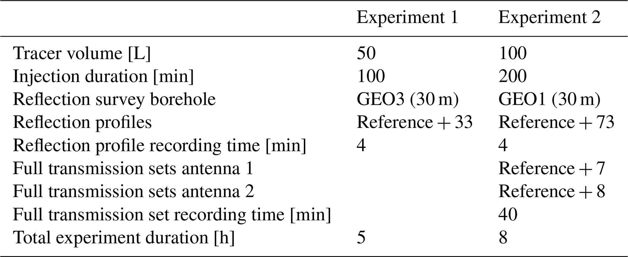
During tracer experiment 1 (100 L injection), GPR data were acquired as a reflection survey with transmitter and receiver antennas placed in the GEO3 borehole, along the borehole length of 30 m (Fig. 3b). The antenna separation was held constant at 1.76 m, and every 10 cm a trace was recorded. The distance was measured with a trigger wheel, and the measurements were recorded while pulling the antenna array upwards, to ensure constant cable tension. The GPR survey lasted for 5 h, but it was partly interrupted due to empty antenna batteries. In total, 34 usable reflection profiles were recorded. Each profile took approximately 4 min to record.
Tracer experiment 2 (200 L injection) was carried out as a combined reflection and transmission survey with four 250 MHz antennas connected as seen in Fig. 3c. One moving antenna set of transmitter and receiver was operated in borehole GEO1, along the borehole length of 30 m, with a fixed distance of 1.76 m. Another static set was used in GEO3 with a fixed distance of 5 m. The trigger wheel was used at GEO1. This setup allowed for a reflection survey carried out in GEO1, during which (as in the previous test) every 10 cm a trace was recorded, again triggered during an upwards motion of the antenna array. In total, 74 usable reflection profiles were recorded. Each profile took approximately 4 min to record.
Simultaneously during experiment 2, a dual-channel transmission survey was conducted, between the static antennas in GEO3 and the moving antennas in GEO1. The two transmission channels (see Fig. 3c) were triggered every 20 cm, while moving the antenna array in GEO1 upwards, with the static antenna array in GEO3 at a fixed position. After each of these recordings, the antenna array in GEO3 was moved to a new position, to record another multi-offset gather. In total, eight different static antenna array positions were occupied in GEO3. To reduce the data acquisition time for the tomography sections, we exploited the potential of the dual-channel setup with two antenna arrays by alternating between two acquisition sets. The positions of the single antennas in the static array, which were separated by 5 m, were chosen to be placed as presented in Table 2. Set 1 covered the positions between 0 and 17.5 m, and Set 2 covered the positions between 5 and 22.5 m, referenced from the bottom of the borehole. The straight ray patterns of the two deployments are shown in Fig. 4b and c. With this procedure, it was possible to use the data either as a more comprehensive data set with all 16 positions, but a lower time resolution, or with only eight positions but a higher time resolution. Both of these options were later used to invert for the change in attenuation.
Table 2Deployment scheme of the static antenna array in GEO3 for the transmission survey. The positions are referenced in meters from the bottom of the borehole.

The acquisition of each of the (full) time-lapse transmission data sets took about 40 min. During that time, eight reflection profiles were recorded simultaneously to the transmission set. The GPR survey lasted for 8 h, but during that time the antennas had to be recharged. In total, one of the two transmission channels recorded eight full sets and the other seven during the experiment. Additionally, one full transmission data set was recorded prior to the tracer injection to serve as the reference data (Fig. 3c).
For a more detailed analysis of the experiment volume, an additional, more comprehensive cross-hole data set, subsequently referred to as baseline data set, was acquired with the same antennas when the experiment volume was unperturbed by any tracer. This data set was acquired with a single antenna set and the MALÅ ProEx console. The static antenna was positioned at every meter in borehole GEO3, and the moving antenna was moved along borehole GEO1 with a trigger interval of 20 cm. The setup can be seen in Fig. 3a and the associated straight ray patterns are shown in Fig. 4a.
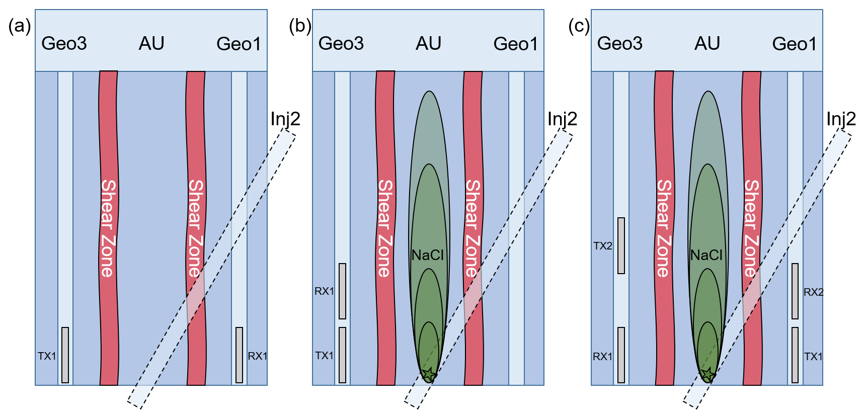
Figure 3Schematic of the acquisition setups for the GPR surveys performed. (a) Setup for baseline data set without tracer injection. (b) Setup for tracer experiment 1 (reflection survey in borehole GEO3). (c) Setup for tracer experiment 2 (combined transmission and reflection survey).
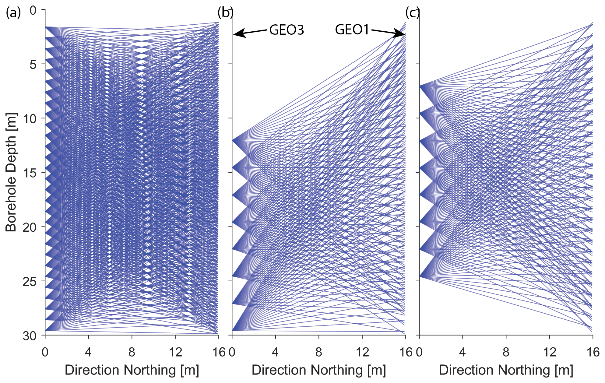
Figure 4Ray coverage for the transmission data sets. Only every fifth ray is plotted. Panel (a) shows the comprehensive baseline data set; (b) and (c) show the two subsets for the time-lapse transmission experiment.
The processing of both the reflection and transmission GPR data sets can be subdivided into two parts. By means of a baseline processing of the reference data sets, acquired prior to the injections, static images of the test volume prior to the tracer injections could be derived. Subsequently, we applied difference processing, such that temporal changes between the individual measurements could be analyzed.
3.1 Baseline reflection imaging
The processing of the reference reflection data sets included relatively few steps. It started with a DC-shift removal, followed by frequency filtering using a 10–50–350–450 MHz Kaiser bandpass window. Then, a singular value decomposition (SVD) filter (e.g., Press, 2002) was applied to remove the direct wave and spurious system ringing effects (removal of the eigenvector associated with the largest eigenvalue). To enhance the amplitudes of later phases, a time-varying gain was applied, consisting of a linear gain proportional to time t to account for spherical spreading and an exponential gain to account for attenuation. Finally, the reflection sections underwent a Kirchhoff migration (from the CREWES Matlab package, Margrave and Lamoureux, 2019) using a constant velocity of 0.12 m/ns that was confirmed by the tomography results and other GPR surveys at the test site (Giertzuch et al., 2020a; Doetsch et al., 2020).
3.2 Difference reflection imaging
The tracer presence in the subsurface is expected to introduce only a minor change in the GPR signals. This is primarily due to the small fracture apertures found in the investigated volume. Therefore, a differencing approach was required to illuminate the signature of the tracer. In principle, calculating the difference between the monitoring and the reference data sets should leave only changes introduced by the tracer, whereas static reflections cancel out. The success of such a procedure is highly dependent on the consistency between the reference and monitoring data sets. Especially in survey areas with several reflectors, as expected in the experiment described here, minor repeatability errors will lead to improper cancellation of the various reflections and may obscure the tracer signal.
Our difference reflection processing closely follows the approach described in detail by Giertzuch et al. (2020a). As for the baseline processing, a DC-shift removal was initially applied to all data sets. Then, a temporal trace alignment was performed to ensure a proper consistency between monitoring and reference data sets. The alignment was performed by calculating a cross-correlation between the reference and monitoring traces and shifting them according to the largest correlation. By up-sampling the traces by a factor of 10, a subsampling interval alignment was possible. After temporal alignment, some elements of the baseline processing were applied to the reference and monitoring data sets (frequency filtering, SVD filtering, and application of a time-varying gain).
Next, a spatial alignment procedure was applied. During acquisition, antenna position inaccuracies may have occurred. Such errors may arise from cable slip, twist and stretch, trigger wheel inaccuracies, or handling mistakes. We applied a cross-correlation and trace-interpolation-based testing scheme for identifying and correcting positioning errors. In the GEO3 data set only minor corrections were required, but in the GEO1 data set, shifts of up to 10 cm had to be applied. The origin of these inconsistencies is unknown.
After applying the processing steps described above, some traces showed artifacts in the form of spiky signals that likely originated from electronic cross talk with other instruments on site. They were removed by replacing them with linearly interpolated values in time and space from adjacent samples and traces. Then, the reference data set was subtracted from the monitoring data sets, which resulted in the GPR difference profiles.
Despite the extensive correction procedures, the difference profiles still exhibited minor artifacts, resulting from improper cancellation of static reflections and diffractions. They were suppressed by again using an SVD filter, with which the eigenvectors associated with the largest five eigenvalues were removed. We found this approach to be more effective than eliminating further singular values in the undifferenced data.
As for the baseline reflection processing, a time-domain Kirchhoff migration was then applied to the difference section. Migrating difference data is useful, since Kirchhoff migration is a linear operator and makes the resulting profiles comparable to migrated GPR sections (Dorn et al., 2012). Furthermore, it helps to reduce ambient noise in the difference data due to focusing of the energy. Finally, a temporal smoothing filter was used to suppress minor random variations between the profiles.
Contrary to what Friedt (2017) and Giertzuch et al. (2020a) have reported, we did not encounter significant sampling rate variations or drifts. This was determined with the procedure described by Giertzuch et al. (2020a) and was unexpected because the same antennas were used in this survey. The greater stability in sampling rate can therefore be likely attributed to the use of the older MALÅ console CU2 instead of the MALÅ ProEx model.
3.3 Baseline tomography
For carrying out the travel time inversions of the baseline transmission data, several pre-processing steps were performed.
-
Determination of the T0 time (emission of the transmitter pulse). The T0 time was estimated by analyzing in-air measurements taken at antenna separations between 3 and 16 m.
-
Sampling rate drift correction. The ProEx console, employed for the transmission measurements, is known to be prone to sampling rate drifts. We accounted for this by acquiring a zero-offset profile (ZOP) prior to the survey. Assuming that the sampling rate remained stable during the relatively short acquisition time of the ZOP, the tomographic (multi-offset) data could be corrected by comparing the travel times of the ZOP with the corresponding traces in the multi-offset data.
-
Anisotropy correction. The recorded cross-hole data showed a slight anisotropy. Since the anisotropy is not expected to vary significantly within the tomographic plane, we judged it appropriate to apply an anisotropy correction procedure, as described in Maurer et al. (2006), and to subsequently employ an isotropic inversion code.
For carrying out the inversions, we considered a ray-based inversion algorithm as described by Maurer et al. (1998), and for the subsequent amplitude inversions, we followed the approach described by Holliger et al. (2001). To account for the underdetermined component of the inversion problem, suitable damping and smoothing constraints were applied.
3.4 Difference attenuation tomography
The presence of an electrically conductive fluid, such as a saline tracer, leads primarily to GPR signal amplitude attenuation and only marginal changes in the travel times of GPR waves. Therefore, we focus here on attenuation tomography. The relative changes in the GPR amplitudes between the reference and monitoring transmission data sets are expected to be relatively small. Therefore, we developed a difference tomography approach, with which minor amplitude variations can be exploited. To assess the amplitude differences, introduced by the presence of the tracer, the monitoring and reference data sets needed to be pre-processed in a consistent manner, such that a valid comparison was possible. For that purpose, we applied the same DC-shift correction as for the reflection data and aligned the monitoring to the reference data with the same temporal trace alignment as described for the reflection data. Additionally, we removed outliers, resulting from faulty traces either in the reference or monitoring data sets.
In the next step, we calculated amplitude difference factors a for each source–receiver pair. They were obtained by performing a linear fit of the first 30 sampling points after the onset of the first arriving wave train:
where are the n sampling points of a reference trace and are the n sampling points of the corresponding monitoring trace. The 30 sampling points correspond approximately to the first wave cycle. Therefore, out-of-plane effects, such as reflections, were largely excluded from our analysis.
From the baseline tomography, the ray path length distribution Lijk (i=1… no. of sources, j=1… no. of receivers, k=1… no. of inversion cells) was available. As outlined in Holliger et al. (2001), ray-based amplitudes can be computed using
where A0 is the source strength, Γi is the transmitter radiation pattern (and coupling), Θj is the receiver radiation pattern (and coupling), and αk is the attenuation in the kth inversion cell. Accordingly, the difference factor aij can be written as
where we distinguish now between the attenuations in the reference and monitoring data sets ( and ) and assume that the ray path distribution Lijk does not change significantly between experiments. As can be seen in Eq. (3), the unknown source strength, the radiation patterns, and the antenna coupling cancel out. Applying the logarithm to Eq. (3) results in
Setting and allows Eq. (4) to be rewritten in a compact matrix vector form as
This represents a linear system of equations that can be solved with a suitable algorithm. As for the baseline tomography, this system of equations includes an underdetermined component, which requires regularization in terms of damping and smoothing.
We applied a two-step inversion scheme on our data. As stated before, the transmission data recording scheme allowed for either the use of a full data set with all 16 positions, but a lower time resolution, or a higher time resolution with only eight positions. First, we considered the larger 16-position data sets to generate the difference attenuation results, whereby the regularization constraints minimized the magnitudes of Δα. Then, we inverted the smaller eight-position data sets that featured a higher temporal resolution, whereby the regularization constraints penalized deviations of Δα. This procedure gave results at the high temporal resolution, practically with the spatial resolution of the larger data set. As longer ray paths over the diagonal source–receiver combinations tend to be less reliable due to radiation characteristics and signal attenuation, we introduced a weighting factor on a in the inversion that was inversely proportional to the ray path lengths, serving as an error estimate.
4.1 Baseline reflection imaging
Figure 5a presents the processed reference profiles for the GEO3 survey and Fig. 5b shows the corresponding profile for the GEO1 survey. Both profiles show numerous overlapping reflections. To aid the visualization of natural (faults) and artificial (boreholes) features, also for the difference images, the most important reflections for these surveys are highlighted with dashed lines. They include reflections from the S3 shear zones, the injection (INJ2) borehole, the PRP1 and PRP2 boreholes, and the other visible GEO boreholes. To ensure a proper identification of the different reflections, the expected reflection GPR responses for the different boreholes were computed using the migration velocity of 0.12 m/ns and compared to the measured reflections. Additionally, the interpretation was based on previous GPR surveys from these boreholes with a higher spatial resolution, as shown in Giertzuch et al. (2020a). Further strong reflections that are not highlighted in the figures could also be identified but were left out here for the sake of image clarity. Both reference profiles show that the relevant regions in the subsurface can be imaged by the GPR surveys. The injection interval in INJ2 that is located between the S3 shear zones and also the PRP boreholes that are known to show breakthroughs for this tracer experiment are visible.
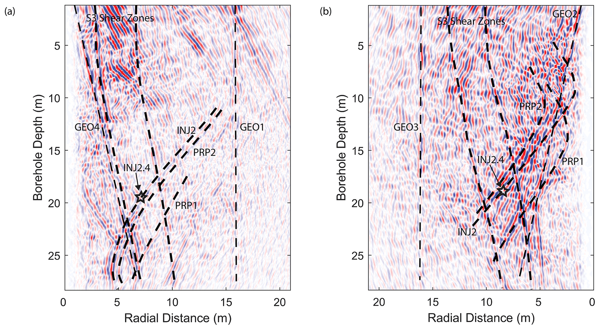
Figure 5Reference profiles for the reflection GPR surveys. (a) Reference from GEO3. (b) Reference from GEO1. Important reflections are indicated by dashed lines and the injection location is marked with a star. Note that the x axis with the distance from the borehole has an opposite direction on the two profiles, such that the geometry is comparable. However, the reflections are not necessarily in the GEO1–GEO3 borehole plane due to the radial ambiguity.
4.2 Difference reflection imaging
The tracer injection started for both experiments at t=0 min and lasted until t=50 min for the GEO3 survey and t=100 min for the GEO1 survey. In Fig. 6, four difference reflection profiles for both of the experiments are presented that were recorded at similar times. The visible tracer reflections are delimited by solid green lines. Additionally, calculated reflection response areas are indicated in the graphs that correspond to relevant borehole intervals and the AU outflow.
In Fig. 6a–d, the difference reflection profiles are presented for the first experiment with reflection GPR monitoring from the GEO3 borehole. At t=12 min after the start of the tracer injection, a clear tracer signal around the injection point is visible. Parts of the tracer already appear to have moved towards the PRP1.3 interval.
At t=41 min, the tracer signal is expressed more strongly, as more tracer has been injected. It has also started to propagate away from the injection point towards the AU tunnel, as the reflections in the image show. Apparently, the tracer has split up at the injection location to propagate towards PRP1.3 and towards the AU tunnel.
At t=126 min, the tracer response around the injection point has disappeared, as formation water was injected after the tracer. The tracer's signature is now visible close to the AU tunnel, but around a borehole depth of 13 m, the tracer signal is strongly reduced or lacking. At t=264 min, the tracer reflection appears strongly around the AU outflow point in the AU tunnel.
Figure 6e–h show four difference reflection profiles for the second experiment with reflection GPR monitoring from the GEO1 borehole. At t=12 min, a clear tracer signal around the injection point is again visible. Parts of the tracer already appear to have moved towards the PRP1.3 interval.
At t=45 min, the tracer signal appears stronger again, as more tracer has been injected. Again, it appears to have split in two directions and also started to propagate away from the injection point towards the AU tunnel.
At t=125 min, the tracer has traveled further towards the AU tunnel. Two flow paths seem to be visible around the injection point and merge at approximately 15 m borehole depth and near the PRP1.3 interval. The reflection signal around a borehole depth of 13 m is only barely visible. At t=264 min, the tracer appears to have reached the AU outflow point. The area around the injection point has now mostly cleared up. Again, formation water was injected after the tracer injection.
In both surveys the calculated reflection positions from the PRP2.2 interval are also reached. This is in good accordance with the conductivity measurements at this interval that showed a breakthrough here at approximately 100 min after tracer injection. However, the radial distance of PRP2.2 to the survey boreholes is similar to the radial distance of the injection point to the survey boreholes. Therefore, the reflections around PRP2.2 and INJ2 cannot be well distinguished, which introduces some uncertainty here. Time-lapse videos of these reflection survey results are available in the Supplement.

Figure 6Time-lapse difference reflection imaging results. Panels (a)–(d) show the results for the experiment conducted in the GEO3 borehole at four different time steps. Panels (e)–(h) show the results at corresponding times for the experiment conducted in the GEO1 borehole. The identified tracer reflections are highlighted in green, while the regions with lower or lacking tracer reflection are marked in red. Note that the x axis with the distance from the borehole has an opposite direction for the two experiments, such that the geometry is better comparable. However, the reflections are not necessarily in the GEO1–GEO3 borehole plane due to the radial ambiguity.
4.3 Baseline velocity and attenuation tomography
Figure 7 shows the inversion results for the velocity and the attenuation of the GPR signal in the tomography plane. Additionally, the S1 and S3 shear zones are depicted within the plane to aid visualization. No dominant structures are visible in the velocity and attenuation images. The velocities vary slightly around 0.12 m/ns, thereby justifying the migration velocity used during the reflection processing. The attenuation is generally low, which can be expected for a granitic host rock.

Figure 7Results of the baseline inversion. Panel (a) shows the velocity result, while (b) shows the attenuation. GEO1 and GEO3 are shown in red; the S1 (red) and S3 (green) shear zones are also depicted for orientation.
4.4 Difference attenuation tomography
The difference attenuation tomography results are presented in Fig. 8 at time steps similar to those shown for the difference images in Fig. 6. Already 20 min after tracer injection, there is a clear increase in attenuation at a depth of approximately 21 m, labeled A. This corresponds to an area close to the injection location, which is slightly below the inversion plane. Therefore, the tracer likely traveled upwards through the inversion plane.
At t=50 min, the tracer signal is more pronounced and extends around the injection location, but no tracer propagation can be seen. After t=125 min, another region with increased attenuation appears at a depth of approximately 8 m, labeled B, and close to the GEO3 borehole at a distance of around 4 m. Later during the experiment, (t=270 min), the attenuation around the injection point (A) appears reduced, but the attenuation around location B has further increased. This corresponds to an expected tracer appearance close to the AU tunnel outflow. Unfortunately, no antenna positions above 7.5 m were available (Fig. 4). Therefore the attenuation increase could not be traced further upwards.
The inversion could be fitted to a root-mean-square (rms) value of approximately 0.05, while the amplitude difference factor can range in theory between 0 and 1. In our data, the factor mainly ranged between 0.7 and 1; however, some data points showed an increased factor of >1. This would correspond to a decrease in attenuation, which was not allowed in the inversion routine; therefore these data were not fitted higher than 1 and thus increase the rms value slightly. The inversions were run for 10 iterations. A time-lapse video of the difference attenuation tomography results is available in the Supplement.

Figure 8Results of the difference attenuation tomography for different time steps after tracer injection. The tracer-induced rise in attenuation can be seen early around a borehole depth of 22 m (labeled A) and later at around 8 m (labeled B).
The results shown in Fig. 6 suffer from an azimuthal ambiguity. Thus, the radial distances away from the boreholes including the GPR antennas are known, but the azimuthal angle from the borehole axis is unknown. For every time step, we could therefore calculate a hollow tubular shape around the borehole axis on which the reflection must have originated, as shown in Fig. 9a. The width (along the radial distance in Fig. 6) of the reflection patterns translates into the wall thickness of the tube, while its length and location along the borehole is defined by the patterns' length and location (along the borehole depth in Fig. 6). It is noteworthy that the extent of these tubes does not represent the actual extent of the reflector but only the extent of possible reflector locations.
The tracer flow path geometry can be assumed to be identical in both experiments, such that a reflection, visible in both experiments, should have occurred at the same locations in the experiment volume. Therefore, we combined the results from the two reflection surveys to reduce the radial ambiguity and confine the tracer localization: the reflection tubes for both experiments could be calculated, and the reflection must have occurred at the intersection of both cylinders. In theory, more than one intersection of two cylinders is possible, and this ambiguity cannot be resolved by using only two boreholes. However, as shown in Fig. 9a, in this study the tubes were mostly intersecting each other only once. Only in the region that also coincides with the reduced tracer reflection in Fig. 6 and the lack of attenuation between features A and B in Fig. 8 do the tubes overlap further, resulting in two intersections: one above the GEO plane and one below.
While the tracer flow path geometry can be assumed to be identical for both experiments, the temporal behavior of the tracer propagation differed due to the different injection protocols. For example, in the first experiment, formation water replaced the tracer already after 50 min and reduced the tracer reflection around the injection point (Fig. 6c). At this time, the reflection was still visible in the second experiment (see Fig. 6g), as the injection lasted for 100 min. To address this, we first combined the reflections for all time steps to generate static tubes of the full tracer flow path for both experiments and analyzed their intersection, as shown in Fig. 9b. The lacking reflection response in the middle of the tracer flow in the GEO3 reflection experiment was estimated and manually interpolated. These estimations were additionally based on the results from Giertzuch et al. (2020a), as the experiments were very similar and no major changes in the flow path were expected. The double intersection described above can be seen in Fig. 9b, as the reconstruction shows the tracer above and/or below the GEO3 plane in the middle of the path that extends towards the AU tunnel.
Once the flow path location is known, the temporal information for both experiments can be analyzed by intersecting the tube sections of a single time step from one experiment with the whole flow path information from the other experiment. This allows generating two time-lapse 3D reconstructions of the tracer propagation for the two experiments. This temporal evolution is presented for the second experiment in Fig. 10a–d along with the results from the difference attenuation tomography. The full time lapse of the reconstruction for both experiments can be found in the Supplement.
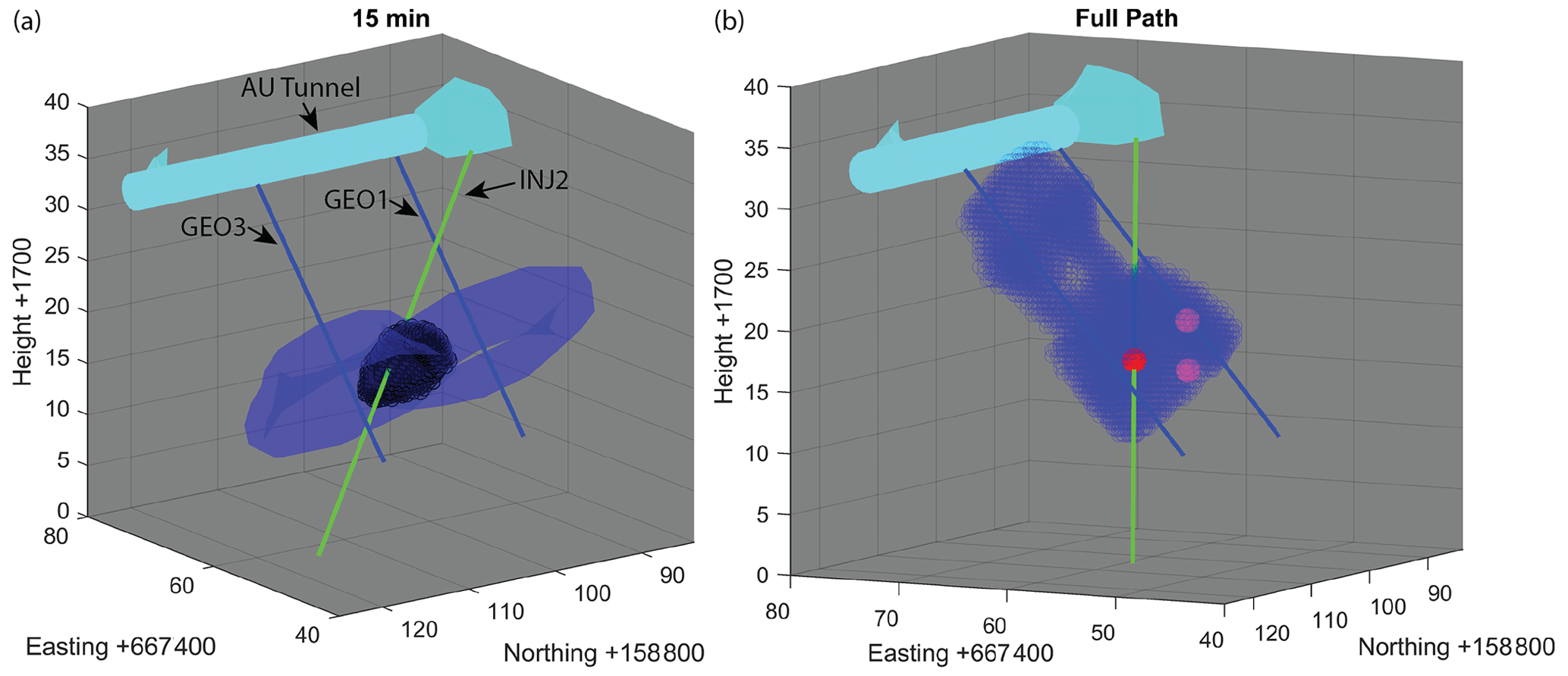
Figure 9Tracer flow path reconstruction and important boreholes (GEO in blue, INJ2 in green). (a) Reflection tubes at 15 min after tracer injection for both surveys in blue and their intersection in black. (b) Fully reconstructed flow path for all time steps. The injection interval is indicated by a red sphere; the two PRP breakthrough locations are indicated by purple spheres.
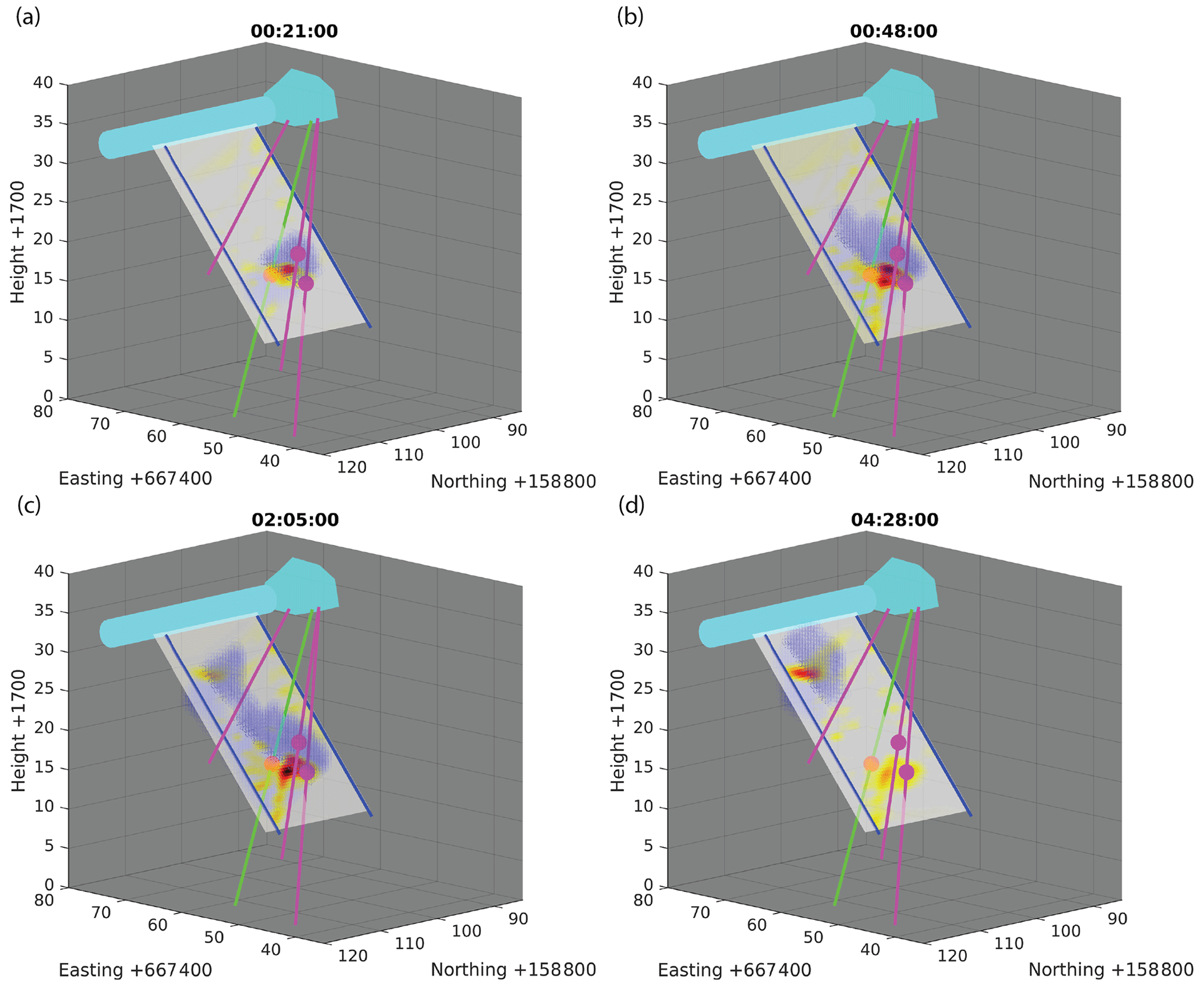
Figure 10Time-lapse tracer flow path reconstruction with tomography results at different time steps after tracer injection. The reconstructed tracer position is shown in blue, the tomography data are presented with the same color scale as in Fig. 8 with scaled transparency. The injection point lies slightly below the tomography plane. The injection interval is indicated by a red sphere; the two PRP breakthrough locations are indicated by purple spheres.
As can be seen in Fig. 9a, the intersection of tubular shapes results in a significant location uncertainty. To provide additional constraints, the attenuation tomography results were included in the analysis. The tomographic images are superimposed in Fig. 10. The tracer is expected to appear in the form of an increased attenuation. In the reflection data, the tracer signature splits into two branches of propagation around the injection point: one in the direction of the AU tunnel and one in the direction of PRP1.3 (Fig. 6a, b, e, f). Therefore, it can be concluded that the branch propagating towards PRP1.3 is associated with the attenuation increase at feature A in Fig. 8. The branch propagating towards the AU tunnel is assumed to stay below the tomographic plane until breaching through it, thereby causing an attenuation increase at feature B in Fig. 8 and further propagating to the AU tunnel outflow.
The resulting tracer flow path is visualized in Fig. 11. Figure 11a again shows the flow path geometry (blue) and the flow directions (black arrows). Additionally, areas where tracer flow seems to be blocked are indicated by an X. The labeled locations A and B refer to the areas of attenuation increase in Fig. 8, indicating that the tracer passed through the GEO plane. The relation of the flow path reconstruction with geological features is visualized in Fig. 11b. It can be inferred that the tracer traveled from the injection location first towards the PRP1.3 interval and the northern S3.2 shear zone and from there propagated further along this shear zone towards the tunnel outflow, as indicated by the black arrows.
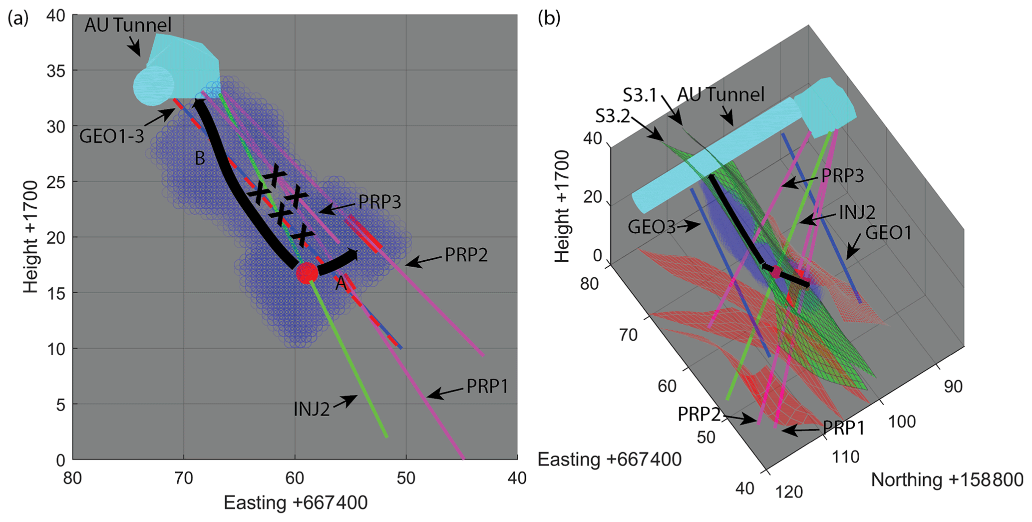
Figure 11Interpretation of the tracer flow path reconstruction. (a) Side view. The tracer indicated by the black arrows passes through the GEO plane (red/blue) at two locations, labeled A and B. (b) Reconstructed flow path along with the shear zones S3 (green) and S1 (red) in the experiment volume. The PRP intervals are indicated in red.
6.1 Interpretation of our results
As shown in Fig. 11, the GPR measurements allow the general tracer flow path regions and flow directions to be delineated. The 3D reconstruction based on the reflection tubes, however, does not represent the tracer position and its extent but should rather be understood as a volume in which tracer reflections are likely to have occurred. Therefore, not every position in the reconstruction was necessarily tracer-filled at some point, but the tracer will have mostly flowed within the extent of the reconstruction. By considering additional data and supplementary information, we will now make an attempt to further constrain the preferential flow path(s) and to validate our results. As shown in the difference reflection images in Fig. 6, and also shown schematically in Fig. 11, the tracer splits up at the injection point into two branches, one traveling towards PRP1.3 and PRP2.2 and the other towards shear zone S3.2 and finally towards the AU tunnel. This was also confirmed by conductivity meter data acquired in the PRP intervals (marked in Figs. 2, 6, and 10). The breakthrough of solute tracers in the PRP intervals and the AU tunnel is also described in dye tracer experiments (Kittilä et al., 2020a, b), with which our findings agree well. Interestingly, the attenuation tomograms, shown in Figs. 8 and 10, do not show a continuous zone associated with the tracer flow, but they exhibit only patches of increased attenuation. This suggests that the tracer must have flowed partially outside of the tomographic plane from feature A to feature B (Fig. 8). This is also confirmed by the 3D reconstruction visible in Figs. 9b and 10. Hence, the question arises of whether the flow path deviates below or above the tomographic plane. As the tracer appears to split at the injection point, only the branch directed towards PRP1.3 is assumed to propagate through the plane, while the other branch apparently stays below the plane until reaching location B in Fig. 11a. Borehole PRP3, which lies entirely above this plane and goes through S3.1 and S3.2 (see Fig. 11), showed no outflow during the experiment, despite multiple identified fractures in the borehole log, and it can therefore be seen as not connected during the timeframe and hydraulic configuration of this experiment. Therefore, we conclude that the tracer flow paths must lie below the tomographic plane. Figure 6 reveals a region of decreased tracer reflectivity in this flow path region (marked red). It is unclear what caused such a decrease. We speculate that an unfavorable fracture orientation or strongly reduced fracture aperture could be the reason. Doetsch et al. (2020) also reported on an area between the S3 shear zones of strongly reduced reflectivity in surface GPR measurements. While it is not entirely clear what causes this decrease and the exact match of the locations is uncertain, these findings appear to be consistent.
Our 4D tracer flow reconstruction agrees with the findings of Brixel et al. (2020a), who described the flow to be strongly fault-controlled, with single cross-fault connections between the S3 shear zones. Our results, however, indicate that the tracer flow towards the tunnel occurs along S3.2 and no flow is seen along S3.1. This observation has so far not been reported in previous publications within the scope of the ISC experiment. Therefore, the GPR experiments appear to not only serve as a visualization but also supply complementary, refining information on the hydraulic system and provide an important additional constraint on the flow and permeability architecture of the fracture system studied.
6.2 Broader implications of our research
The methods described here should be transferable to a variety of research fields and experiment sites, where detailed process localization is necessary and direct observations are not an option. A successful application primarily depends on the host medium, the accessibility, and the scale of the research site: the electrical conductivity of the host rock needs to be sufficiently low for signal propagation, and for using saline tracers, a sufficiently strong contrast towards formation water needs to be ensured. Moreover, different GPR monitoring locations are needed for the localization. Two boreholes were used in our study, but a combination of surface GPR in access tunnels or a combination of surface and borehole GPR could be possible. Furthermore, the research site and the processes monitored must be resolvable by GPR; hence the scale of both the site and the processes needs to be considered.
Our methodology was developed within the scope of geothermal energy research, on an intermediate (decameter) scale between laboratory and full-scale application. While a transfer towards full-scale deep geothermal energy exploitation will be challenging, applications within hectometer-scale research projects are reasonable. Such a project is, for example, currently ongoing in the Bedretto Laboratory (http://www.bedrettolab.ethz.ch, last access: 15 June 2021) in Switzerland (Gischig et al., 2020). Intermediate-scale projects are employed to investigate the complex seismo-hydromechanical interaction and therefore depend on a detailed flow system characterization. Further, Shakas et al. (2020) have recently used 100 MHz borehole antennas for time-lapse difference GPR to monitor aperture changes (and thus permeability changes) during hydraulic stimulation, thereby proving that the requirements for difference imaging can be met on those scales. Our spatial reconstruction approach could be transferred to such experiments, where instead of tracer fluid propagation the geomechanical changes could be monitored and localized by time-lapse GPR.
Experiments in which substantial changes in the flow paths can be expected, for instance in pre- and post-stimulation comparisons for reservoir creation, could be of special interest. The methods described in this study could provide a valuable tool to assess and visualize how and to what extent the subsurface fluid flow was affected by stimulation.
We judge our methodology to be useful for further applications where flow paths or their changes are of relevance. Examples include tracing of fluid contaminants, related to radioactive waste repositories (such as the Äspö Hard Rock Laboratory, e.g., Cosma et al., 2001), or civil engineering projects.
Our tracer reconstruction also shows that fluid flow is confined to a limited number of fractures (compared to the total fractures encountered during drilling). Such information can therefore help parameterize site-specific numerical models of flow and transport in crystalline rock, where identifying permeable fractures that control the flow behavior of the rock is important.
In this contribution, we have presented results from two borehole GPR experiments that were performed to monitor saline tracer flow in weakly fractured crystalline rock with small-aperture fractures. Both experiments had a similar tracer injection protocol, but they were used to acquire complementary data sets. A geometrical reconstruction approach was applied that successfully overcame the radial ambiguity in the data and resulted in a 4D tracer flow reconstruction. This reconstruction was validated with the known tracer breakthroughs from conductivity meters that were installed in the experiment volume.
The GPR transmission data were analyzed using a novel time-lapse difference attenuation tomography routine that revealed clear areas of attenuation introduced by the tracer in the tomography plane. The results matched those from the reflection analysis well and further strengthen the validity of our approach.
We judge our methodology to be useful to a wide range of applications well beyond flow processes in fractured crystalline rock. Examples include tracing fluid contaminants in the subsurface and monitoring nuclear waste repositories. Generally, it needs to be ensured that the GPR method is applicable (i.e., the electrical conductivities of the host rock need to be sufficiently low). Furthermore, it must be ensured that the measurements can be performed quickly enough, such that the temporal behavior of the process of interest can be resolved adequately. In the field of geothermal research, we judge that applying our methodology of spatial reconstruction to GPR monitoring during stimulation experiments could strongly improve our understanding of stimulation effects in fracture networks.
The data are available under https://doi.org/10.3929/ethz-b-000456232 (Giertzuch et al., 2020b).
The supplement related to this article is available online at: https://doi.org/10.5194/se-12-1497-2021-supplement.
PLG performed the conceptualization, investigation, and formal analysis and wrote the original draft. JD supported the conceptualization, investigation, and formal analysis, supervised the study, acquired funding, and performed writing (review and editing). AS supported the formal analysis and performed writing (review and editing). MJ supported the investigation and performed writing (review and editing). BB supported the investigation and performed writing (review and editing). HM supported the formal analysis, supervised the study, and performed writing (review and editing).
The authors declare that they have no conflict of interest.
We would like to thank George Tsoflias and an anonymous reviewer for their review and comments on this paper. The ISC is a project of the Deep Underground Laboratory at ETH Zurich, established by the Swiss Competence Center for Energy Research – Supply of Electricity (SCCER-SoE) with the support of the Swiss Commission for Technology and Innovation (CTI). The Grimsel Test Site is operated by Nagra, the National Cooperative for the Disposal of Radioactive Waste. We are indebted to Nagra for hosting the ISC experiment in their GTS facility and to the Nagra technical staff for on-site support.
This research has been supported by the Schweizerischer Nationalfonds zur Förderung der Wissenschaftlichen Forschung (grant no. 200021 169894). Funding for the ISC project was provided by the ETH Foundation with grants from Shell, EWZ, and by the Swiss Federal Office of Energy through a P&D grant.
This paper was edited by Ulrike Werban and reviewed by George Tsoflias and one anonymous referee.
Allroggen, N. and Tronicke, J.: Attribute-Based Analysis of Time-Lapse Ground-Penetrating Radar Data, Geophysics, 81, H1–H8, https://doi.org/10.1190/geo2015-0171.1, 2016. a
Allroggen, N., Beiter, D., and Tronicke, J.: Ground-Penetrating Radar Monitoring of Fast Subsurface Processes, Geophysics, 85, A19–A23, https://doi.org/10.1190/geo2019-0737.1, 2020. a
Amann, F., Gischig, V., Evans, K., Doetsch, J., Jalali, R., Valley, B., Krietsch, H., Dutler, N., Villiger, L., Brixel, B., Klepikova, M., Kittilä, A., Madonna, C., Wiemer, S., Saar, M. O., Loew, S., Driesner, T., Maurer, H., and Giardini, D.: The seismo-hydromechanical behavior during deep geothermal reservoir stimulations: open questions tackled in a decameter-scale in situ stimulation experiment, Solid Earth, 9, 115–137, https://doi.org/10.5194/se-9-115-2018, 2018. a, b, c
Andričević, R. and Cvetković, V.: Evaluation of Risk from Contaminants Migrating by Groundwater, Water Resour. Res., 32, 611–621, https://doi.org/10.1029/95WR03530, 1996. a
Brewster, M. L. and Annan, A. P.: Ground-penetrating Radar Monitoring of a Controlled DNAPL Release: 200 MHz Radar, Geophysics, 59, 1211–1221, https://doi.org/10.1190/1.1443679, 1994. a
Brixel, B., Klepikova, M., Jalali, M., Amann, F., and Loew, S.: High-Resolution Cross-Borehole Thermal Tracer Testing in Granite: Preliminary Field Results, Geophys. Res. Abstr., EGU-16756, EGU General Assembly 2017, Vienna, Austria, 2017. a
Brixel, B., Klepikova, M., Jalali, M. R., Lei, Q., Roques, C., Kriestch, H., and Loew, S.: Tracking Fluid Flow in Shallow Crustal Fault Zones: 1. Insights From Single-Hole Permeability Estimates, J. Geophys. Res.-Sol. Ea., 125, e2019JB018200, https://doi.org/10.1029/2019JB018200, 2020a. a, b, c, d
Brixel, B., Klepikova, M., Lei, Q., Roques, C., Jalali, M. R., Krietsch, H., and Loew, S.: Tracking Fluid Flow in Shallow Crustal Fault Zones: 2. Insights From Cross-Hole Forced Flow Experiments in Damage Zones, J. Geophys. Res.-Sol. Ea., 125, e2019JB019108, https://doi.org/10.1029/2019JB019108, 2020b. a, b, c
Brown, D. W., Duchane, D. V., Heiken, G., and Hriscu, V. T.: Mining the Earth's Heat: Hot Dry Rock Geothermal Energy, Springer Berlin Heidelberg, Berlin, Heidelberg, https://doi.org/10.1007/978-3-540-68910-2, 2012. a
Cosma, C., Olsson, O., Keskinen, J., and Heikkinen, P.: Seismic Characterization of Fracturing at the Äspö Hard Rock Laboratory, Sweden, from the Kilometer Scale to the Meter Scale, Int. J. Rock Mech. Min., 38, 859–865, https://doi.org/10.1016/S1365-1609(01)00051-X, 2001. a
Cvetkovic, V., Painter, S., Outters, N., and Selroos, J. O.: Stochastic Simulation of Radionuclide Migration in Discretely Fractured Rock near the Äspö Hard Rock Laboratory, Water Resour. Res., 40, W02404, https://doi.org/10.1029/2003WR002655, 2004. a
Day-Lewis, F. D., Lane, J. W., Harris, J. M., and Gorelick, S. M.: Time-Lapse Imaging of Saline-Tracer Transport in Fractured Rock Using Difference-Attenuation Radar Tomography, Water Resour. Res., 39, 1290, https://doi.org/10.1029/2002WR001722, 2003. a
de La Bernardie, J., de Dreuzy, J.-R., Bour, O., and Lesueur, H.: Synthetic Investigation of Thermal Storage Capacities in Crystalline Bedrock through a Regular Fracture Network as Heat Exchanger, Geothermics, 77, 130–138, https://doi.org/10.1016/j.geothermics.2018.08.010, 2019. a
Doetsch, J., Krietsch, H., Lajaunie, M., Schmelzbach, C., Maurer, H., and Amann, F.: GPR Imaging of Shear Zones in Crystalline Rock, in: 2017 9th International Workshop On Advanced Ground Penetrating Radar (IWAGPR), 1–5, IEEE, Edinburgh, UK, 2017. a
Doetsch, J., Gischig, V., Krietsch, H., Villiger, L., Amann, F., Dutler, N., Jalali, R., Brixel, B., Klepikova, M., Roques, C., Giertzuch, P.-L., Kittilä, A., and Hochreutener, R.: Grimsel ISC Experiment Description, Report, ETH Zurich, https://doi.org/10.3929/ethz-b-000310581, 2018. a, b
Doetsch, J., Krietsch, H., Schmelzbach, C., Jalali, M., Gischig, V., Villiger, L., Amann, F., and Maurer, H.: Characterizing a decametre-scale granitic reservoir using ground-penetrating radar and seismic methods, Solid Earth, 11, 1441–1455, https://doi.org/10.5194/se-11-1441-2020, 2020. a, b, c, d
Dorn, C., Linde, N., Le Borgne, T., Bour, O., and Baron, L.: Single-Hole GPR Reflection Imaging of Solute Transport in a Granitic Aquifer, Geophys. Res. Lett., 38, L08401, https://doi.org/10.1029/2011GL047152, 2011. a
Dorn, C., Linde, N., Le Borgne, T., Bour, O., and Klepikova, M.: Inferring Transport Characteristics in a Fractured Rock Aquifer by Combining Single-Hole Ground-Penetrating Radar Reflection Monitoring and Tracer Test Data, Water Resour. Res., 48, W11521, https://doi.org/10.1029/2011WR011739, 2012. a
Friedt, J.: Passive Cooperative Targets for Subsurface Physical and Chemical Measurements: A Systems Perspective, IEEE Geosci. Remote Sens. Lett., 14, 821–825, https://doi.org/10.1109/LGRS.2017.2681901, 2017. a
Giertzuch, P.-L., Doetsch, J., Jalali, M., Shakas, A., Schmelzbach, C., and Maurer, H.: Time-Lapse Ground Penetrating Radar Difference Reflection Imaging of Saline Tracer Flow in Fractured Rock, Geophysics, 85, H25–H37, https://doi.org/10.1190/geo2019-0481.1, 2020a. a, b, c, d, e, f, g, h, i, j, k, l
Giertzuch, P.-L., Doetsch, J., Brixel, B., and Jalali, M.: Single-Hole and Cross-Hole Time-Lapse GPR 250MHz Borehole Dataset during Salt Tracer injection, ETH Zurich [data set], https://doi.org/10.3929/ethz-b-000456232, 2020b. a
Gischig, V. S., Giardini, D., Amann, F., Hertrich, M., Krietsch, H., Loew, S., Maurer, H., Villiger, L., Wiemer, S., Bethmann, F., Brixel, B., Doetsch, J., Doonechaly, N. G., Driesner, T., Dutler, N., Evans, K. F., Jalali, M., Jordan, D., Kittilä, A., Ma, X., Meier, P., Nejati, M., Obermann, A., Plenkers, K., Saar, M. O., Shakas, A., and Valley, B.: Hydraulic Stimulation and Fluid Circulation Experiments in Underground Laboratories: Stepping up the Scale towards Engineered Geothermal Systems, Geomechanics for Energy and the Environment, 24, 100175, https://doi.org/10.1016/j.gete.2019.100175, 2020. a
Hawkins, A. J., Becker, M. W., and Tsoflias, G. P.: Evaluation of Inert Tracers in a Bedrock Fracture Using Ground Penetrating Radar and Thermal Sensors, Geothermics, 67, 86–94, https://doi.org/10.1016/j.geothermics.2017.01.006, 2017. a
Holliger, K., Musil, M., and Maurer, H.: Ray-Based Amplitude Tomography for Crosshole Georadar Data: A Numerical Assessment, J. Appl. Geophys., 47, 285–298, https://doi.org/10.1016/S0926-9851(01)00072-6, 2001. a, b
Jalali, M., Gischig, V., Doetsch, J., Näf, R., Krietsch, H., Klepikova, M., Amann, F., and Giardini, D.: Transmissivity Changes and Microseismicity Induced by Small-Scale Hydraulic Fracturing Tests in Crystalline Rock, Geophys. Res. Lett., 45, 2265–2273, https://doi.org/10.1002/2017GL076781, 2018a. a
Jalali, M., Klepikova, M., Doetsch, J., Krietsch, H., Brixel, B., Dutler, N., Gischig, V., and Amann, F.: A Multi-Scale Approach to Identify and Characterize the Preferential Flow Paths of a Fractured Crystalline Rock, in: 2nd International Discrete Fracture Network Engineering Conference, American Rock Mechanics Association, Seattle, Washington, USA, 2018b. a
Jalali, R., Roques, C., Leresche, S., Brixel, B., Giertzuch, P.-L., Doetsch, J., Schopper, F., Dutler, N., Villiger, L., Krietsch, H., Gischig, V., Valley, B., and Amann, F.: Evolution of Preferential Flow Paths during the In-Situ Stimulation and Circulation (ISC) Experiment – Grimsel Test Site, Geophys. Res. Abstr., EGU2019-12400, EGU General Assembly 2019, Vienna, Austria, https://doi.org/10.3929/ethz-b-000352149, 2019. a
Jol, H. M. (Ed.): Ground Penetrating Radar: Theory and Applications, 1st Edn., Elsevier Science, Amsterdam, 2009. a
Kittilä, A., Jalali, M. R., Evans, K. F., Willmann, M., Saar, M. O., and Kong, X.-Z.: Field Comparison of DNA-Labeled Nanoparticle and Solute Tracer Transport in a Fractured Crystalline Rock, Water Resour. Res., 55, 6577–6595, https://doi.org/10.1029/2019WR025021, 2019. a
Kittilä, A., Jalali, M., Saar, M. O., and Kong, X.-Z.: Solute Tracer Test Quantification of the Effects of Hot Water Injection into Hydraulically Stimulated Crystalline Rock, Geothermal Energy, 8, 17, https://doi.org/10.1186/s40517-020-00172-x, 2020a. a, b, c, d
Kittilä, A., Jalali, M. R., Somogyvári, M., Evans, K. F., Saar, M. O., and Kong, X. Z.: Characterization of the Effects of Hydraulic Stimulation with Tracer-Based Temporal Moment Analysis and Tomographic Inversion, Geothermics, 86, 101820, https://doi.org/10.1016/j.geothermics.2020.101820, 2020b. a, b, c, d
Klenk, P., Jaumann, S., and Roth, K.: Quantitative high-resolution observations of soil water dynamics in a complicated architecture using time-lapse ground-penetrating radar, Hydrol. Earth Syst. Sci., 19, 1125–1139, https://doi.org/10.5194/hess-19-1125-2015, 2015. a
Krietsch, H., Doetsch, J., Dutler, N., Jalali, M., Gischig, V., Loew, S., and Amann, F.: Comprehensive Geological Dataset Describing a Crystalline Rock Mass for Hydraulic Stimulation Experiments, Scientific Data, 5, 180269, https://doi.org/10.1038/sdata.2018.269, 2018. a, b, c, d, e
Lázaro-Mancilla, O. and Gómez-Treviño, E.: Synthetic Radargrams from Electrical Conductivity and Magnetic Permeability Variations, J. Appl. Geophys., 34, 283–290, https://doi.org/10.1016/0926-9851(96)00005-5, 1996. a
Mangel, A. R., Moysey, S. M. J., and Bradford, J.: Reflection tomography of time-lapse GPR data for studying dynamic unsaturated flow phenomena, Hydrol. Earth Syst. Sci., 24, 159–167, https://doi.org/10.5194/hess-24-159-2020, 2020. a
Margrave, G. F. and Lamoureux, M. P.: Numerical Methods of Exploration Seismology: With Algorithms in MATLAB, Cambridge University Press, Cambridge, New York, NY, 2019. a
Maurer, H., Holliger, K., and Boerner, D. E.: Stochastic Regularization: Smoothness or Similarity?, Geophys. Res. Lett., 25, 2889–2892, https://doi.org/10.1029/98GL02183, 1998. a
Maurer, H., Schubert, S. I., Bächle, F., Clauss, S., Gsell, D., Dual, J., and Niemz, P.: A Simple Anisotropy Correction Procedure for Acoustic Wood Tomography, Holzforschung, 60, 567–573, https://doi.org/10.1515/HF.2006.094, 2006. a
National Research Council: Rock Fractures and Fluid Flow: Contemporary Understanding and Applications, The National Academies Press, Washington, DC, https://doi.org/10.17226/2309, 1996. a
Niva, B., Olsson, O., and Blümling, P.: Grimsel Test Site: Radar Crosshole Tomography with Application to Migration of Saline Tracer through Fracture Zones, Tech. Rep. NTB 88-31, Nagra, Baden, 1988. a
Press, W. H. (Ed.): Numerical Recipes in C++: The Art of Scientific Computing, 2nd Edn., Cambridge University Press, Cambridge, UK, New York, 2002. a
Shakas, A., Linde, N., Baron, L., Bochet, O., Bour, O., and Le Borgne, T.: Hydrogeophysical Characterization of Transport Processes in Fractured Rock by Combining Push-Pull and Single-Hole Ground Penetrating Radar Experiments, Water Resour. Res., 52, 938–953, https://doi.org/10.1002/2015WR017837, 2016. a
Shakas, A., Linde, N., Baron, L., Selker, J., Gerard, M.-F., Lavenant, N., Bour, O., and Le Borgne, T.: Neutrally Buoyant Tracers in Hydrogeophysics: Field Demonstration in Fractured Rock, Geophys. Res. Lett., 44, 3663–3671, https://doi.org/10.1002/2017GL073368, 2017. a
Shakas, A., Maurer, H., Giertzuch, P.-L., Hertrich, M., Giardini, D., Serbeto, F., and Meier, P.: Permeability Enhancement From a Hydraulic Stimulation Imaged With Ground Penetrating Radar, Geophys. Res. Lett., 47, e2020GL088783, https://doi.org/10.1029/2020GL088783, 2020. a
Trinks, I., Stümpel, H., and Wachsmuth, D.: Monitoring Water Flow in the Unsaturated Zone Using Georadar, First Break, 19, https://doi.org/10.1046/j.1365-2397.2001.00228.x, 2001. a
Tsoflias, G. P. and Becker, M. W.: Ground-Penetrating-Radar Response to Fracture-Fluid Salinity: Why Lower Frequencies Are Favorable for Resolving Salinity Changes, Geophysics, 73, J25–J30, https://doi.org/10.1190/1.2957893, 2008. a