the Creative Commons Attribution 4.0 License.
the Creative Commons Attribution 4.0 License.
 | 12 Jan 2021
Monitoring surface deformation of deep salt mining in Vauvert (France), combining InSAR and leveling data for multi-source inversion
Séverine Liora Furst
Samuel Doucet
Philippe Vernant
Cédric Champollion
Jean-Louis Carme
The salt mining industrial exploitation located in Vauvert (France) has been injecting water at high pressure into wells to dissolve salt layers at depth. The extracted brine has been used in the chemical industry for more than 30 years, inducing a subsidence of the surface. Yearly leveling surveys have monitored the deformation since 1996. This dataset is supplemented by synthetic aperture radar (SAR) images, and since 2015, global navigation satellite system (GNSS) data have also continuously measured the deformation. New wells are regularly drilled to carry on with the exploitation of the salt layer, maintaining the subsidence. We make use of this careful monitoring by inverting the geodetic data to constrain a model of deformation. As InSAR and leveling are characterized by different strengths (spatial and temporal coverage for InSAR, accuracy for leveling) and weaknesses (various biases for InSAR, notably atmospheric, very limited spatial and temporal coverage for leveling), we choose to combine SAR images with leveling data, to produce a 3-D velocity field of the deformation. To do so, we develop a two-step methodology which consists first of estimating the 3-D velocity from images in ascending and descending acquisition of Sentinel 1 between 2015 and 2017 and second of applying a weighted regression kriging to improve the vertical component of the velocity in the areas where leveling data are available. GNSS data are used to control the resulting velocity field. We design four analytical models of increasing complexity. We invert the combined geodetic dataset to estimate the parameters of each model. The optimal model is made of 21 planes of dislocation with fixed position and geometry. The results of the inversion highlight two behaviors of the salt layer: a major collapse of the salt layer beneath the extracting wells and a salt flow from the deepest and most external zones towards the center of the exploitation.
- Article
(14876 KB) - Full-text XML
- BibTeX
- EndNote


Rock salt (halite) is a sedimentary rock formed by the evaporation of seawater under specific conditions at different geological times. Halite deposits are located underground or inside mountains, though some can also be found on the surface in arid regions. They mainly contain crystals of sodium chlorite (NaCl) but can also include impurities such as clay, anhydrite, or calcite. The distribution of salt deposits worldwide is very localized, spread over areas ranging from a few up to several hundred square kilometers. In Europe, countries such as Germany, Denmark, and the Netherlands have a large amount of salt (Gillhaus and Horvath, 2008). The buried layers of rock salt can be dissolved by injecting water during the so-called solution mining process. This process is used to extract salt in the form of brine (for the chemical industry). More commonly, solution mining aims at creating salt caverns for the storage of fossil fuels such as natural gas, oil, and petroleum products (refined fuels, liquefied gas) but also for the storage of hydrogen and compressed air (Donadei and Schneider, 2016).
The difference between geostatic pressure and brine (or hydrocarbons) at cavern depth produces a change in stress equilibrium that leads to elastic and visco-elastic deformation of the surrounding medium (Bérest and Brouard, 2003; Bérest et al., 2006, 2012). The instantaneous (i.e., elastic) subsidence is due to the change in stress because of the excavation. The latter is relatively small (up to a few centimeters) for most salt and potash mines (Van Sambeek, 1993). Furthermore, a time-dependent subsidence also occurs, due to salt creep related to caverns opening. This long-term subsidence continues until the cavern volume vanishes, reaching large deformation (1 m or more) over tens or hundreds of years (Van Sambeek, 1993). These deferred dynamic surface deformations may result in damage to infrastructures (e.g., pipelines, roads, buildings, railways) in the vicinity of the exploitation. Therefore, to mitigate these potential effects, long-term monitoring of the mining activities is usually mandated by governments. In this study, we focus on the particular monitoring of the deformation induced by rock salt mining in Vauvert (southern France) using geodetic instruments and techniques. The extraction is performed in some of the world's deepest boreholes in salt reservoirs. The subsidence has been monitored since 1996 using (1) leveling survey (IGN, Institut Géographique National) and (2) SAR (synthetic aperture radar) images acquired by various satellite missions (ERS, ENVISAT, SENTINEL). With no further processing, only 1-D displacements (along the line of sight of the satellite or the vertical component for leveling) can be described. A previous study from Raucoules et al. (2003) has identified an 8 km diameter subsidence bowl centered on the eastern part of the exploitation. They suggest a maximum subsidence rate of 22 mm yr−1 based on the differential SAR interferometry (DInSAR) technique applied to ERS-1 and ERS-2 images from 1993 to 1999. Nevertheless, one can postulate that the surface deformation induced by the salt extraction should include 3-D displacements rates, including horizontal displacements either due to the salt flow or to the centripetal displacement associated with the subsidence. Hence, four continuous global navigation satellite system (cGNSS) stations were installed in 2015 (one station) and 2016 (three stations) to measure the local 3-D surface velocities.
Along with spatially dense InSAR and leveling data, a complete description of the 3-D surface displacement rates can be assessed by combining the geodetic datasets. Indeed, all three geodetic techniques measuring the subsidence in Vauvert are complementary regarding their spatial and temporal attributes. The combination of deformation data measured according to different geometries is not trivial. The displacement values are indeed projected along the line of sight of the satellite for InSAR, along the vertical for leveling, and in 3-D for GNSS. Different combination techniques have already been tested at different stages of data processing: first, different satellite acquisition geometries (e.g., ascending, descending, and ascending of parallel orbit) can be used to estimate the three components of the displacement (Wright et al., 2004). This implies that interferograms may cover slightly different time periods including information on the source at different time (Peltier et al., 2017). Second, combining data of different temporal and spatial sampling rates can be done using methods of interpolation such as Gaussian process regression (kriging). These methods assume a constant deformation rate over the observed period but also that the data sampling is statistically representative (spatially and temporally) of the area of interest. For instance, Fuhrmann et al. (2015) developed a methodology to calculate and combine linear velocity rates from InSAR, leveling, and GNSS data measured in the Upper Rhine graben. InSAR, GNSS, and leveling velocities are interpolated independently by ordinary kriging. Finally, these interpolated datasets are merged by a least squares adjustment enabling the estimate of the north, east, and vertical components of the velocity field. Similarly, Lu et al. (2015) analyze leveling, permanent scatterers (PSs), and cross (between both datasets) variograms over the Choushui River fluvial plain in Taiwan. However, these methods are not suitable for the current study. Indeed, the interpolation methods (kriging and co-kriging) implicitly assume that the sample is statistically representative (spatially and temporally) of the deformation field. InSAR kriging works for most cases where the density of points allows the interpretation of surface displacements. When several measurement techniques (GPS, leveling, tacheometry, or inclinometry) are statistically representative of the deformation (spatially and temporally), the co-kriging method can be implemented. In this study, leveling lines measure the vertical displacement and complement InSAR data. We implement a methodology to estimate the 3-D velocity field from the combination of InSAR and leveling data. This 3-D velocity field provides a unique dataset revealing significant horizontal velocities. Considering the small number and the late installation of cGNSS stations (only partially matching the InSAR period), the resulting 3-D velocities are not consistent in space and time. Therefore, they were not used to constrain the InSAR-based velocity field but only to control the accuracy of the final velocity field in a first approximation.
From the combined velocity field, models of the salt layer (e.g., analytical, numerical, or geomechanical) can be derived in order to improve the brine productivity and to predict the evolution of subsidence. A software has already been developed for the Solution Mining Research Institute to evaluate and predict surface subsidence over underground openings (Van Sambeek, 1993). Although this model accounts for three-dimensional geometry, the distribution over time of the openings, and salt creep, it does not include the surface data, such as displacements or velocities. The model is used to simulate ground subsidence above solution-mined caverns or dry mines and not to infer source parameters. Instead, geodetic data measured in Vauvert can be inverted to model deep sources of strain similarly to model sources resulting from magmatic activities (e.g., Peltier et al., 2007; Camacho et al., 2011; Galgana et al., 2014), CO2 injection (e.g., Vasco et al., 2008), stimulated reservoirs (e.g., Astakhov et al., 2012), or gas reservoir compartmentalization (e.g., Fokker et al., 2012). In order to find the optimal model explaining the 3-D velocity field, we consider four analytical models of different configurations and increasing complexity: a single point source of varying position and volume variation (Mogi, 1958), a 2-D plane of dislocation (Okada, 1992), and two collections of 21 and 28 planes of dislocation (Okada, 1992) with fixed position, depth, orientation, and geometry. The point source implies a simple pressurized source inducing symmetrical vertical displacements of the surface. The horizontal displacements modeled by the point source are induced by the centripetal displacement associated with the subsidence. Contrary to the pressurized source, planar dislocation allows for shear motion in addition to tensile motion of the plane and can therefore capture more complex processes such as salt flow. Besides, such models are also more representative of deep salt layers. The inversion of the 3-D velocity field allows us to constrain models of the salt layer and to give a hypothesis for the origin of the horizontal displacements.
In our study, we aim at characterizing the deformation of salt reservoir using Sentinel-1 images, leveling lines, and GNSS data. We propose a two-step methodology to combine geodetic data measuring the bowl of subsidence induced by the salt extraction in Vauvert (Doucet, 2018). In the first step, we estimate the three components of the subsidence observed in Vauvert from InSAR data. In a second step, we use a regression-kriging technique, to constrain the vertical component of the displacement using leveling data. This latter is then inverted using a gradient-based method to characterize the parameters of each models and to define the best model of the salt layer regarding the geodetic dataset. Results are interpreted and discussed taking into account production data from the operator company and geological and geophysical complementary information.
2.1 Geological setting
The salt deposit of Vauvert is located on the NW margin of the on-shore half graben of the extensional Camargue basin in southern France. This graben results from the Oligo-Aquitanian rifting of the margin during the Mediterranean Sea expansion (Séranne et al., 1995). This extensional phase lasts from 30 to 15 Ma and affects the rim of the Alpine belt (Pyrenees, Languedoc, Gulf of Lion, Camargue, Valentinois, Bresse, Rhine plain). The NE–SW-oriented basins are controlled by the SE-dipping Nîmes normal fault (Fig. 1). Camargue basin contains up to 4000 m of syn-rift sediments which overlay a substratum of carbonates from the Lower Cretaceous (130 Ma). The rapid Oligo-Aquitanian sedimentation formed a succession of continental to lagoonal series generally found between 900 and 4900 m at depth (Fig. 1; Valette and Benedicto, 1995):
-
the clay series brings together two sub-series – the “gray series” (2000 m thick of deposit of clay, sand, limestone, marl, conglomerate, and lignite) and the “red series” (200 m of clay and gypsiferous marls with several intervals of marl and sand from palustrine environment);
-
The saliferous series (900 m thick) with four formations – the infra-saliferous, the lower saliferous, the intermediate marl, and the upper saliferous formations; these formations lie between 1500 and 3000 m deep and are affected by normal faults and two thrust surfaces, i.e., decollements D1 and D2 (Fig. 1); the salt layers dip at 30 ± 5∘;
-
The marine clay series range from 800 to 1500 m thick and correspond to three sequences of Aquitanian deposits, mainly composed of clay with intervals of limestones, sandstones, or layers of dolomite.
During the Miocene crustal spreading, syn-rift sediments were covered by transgressive Burdigalian marine sediments and coastal molasses before being uplifted and eroded during the Messinian event (Valette and Benedicto, 1995). The whole formation was finally overlaid by one last stage of sedimentation occurring during the Pliocene.
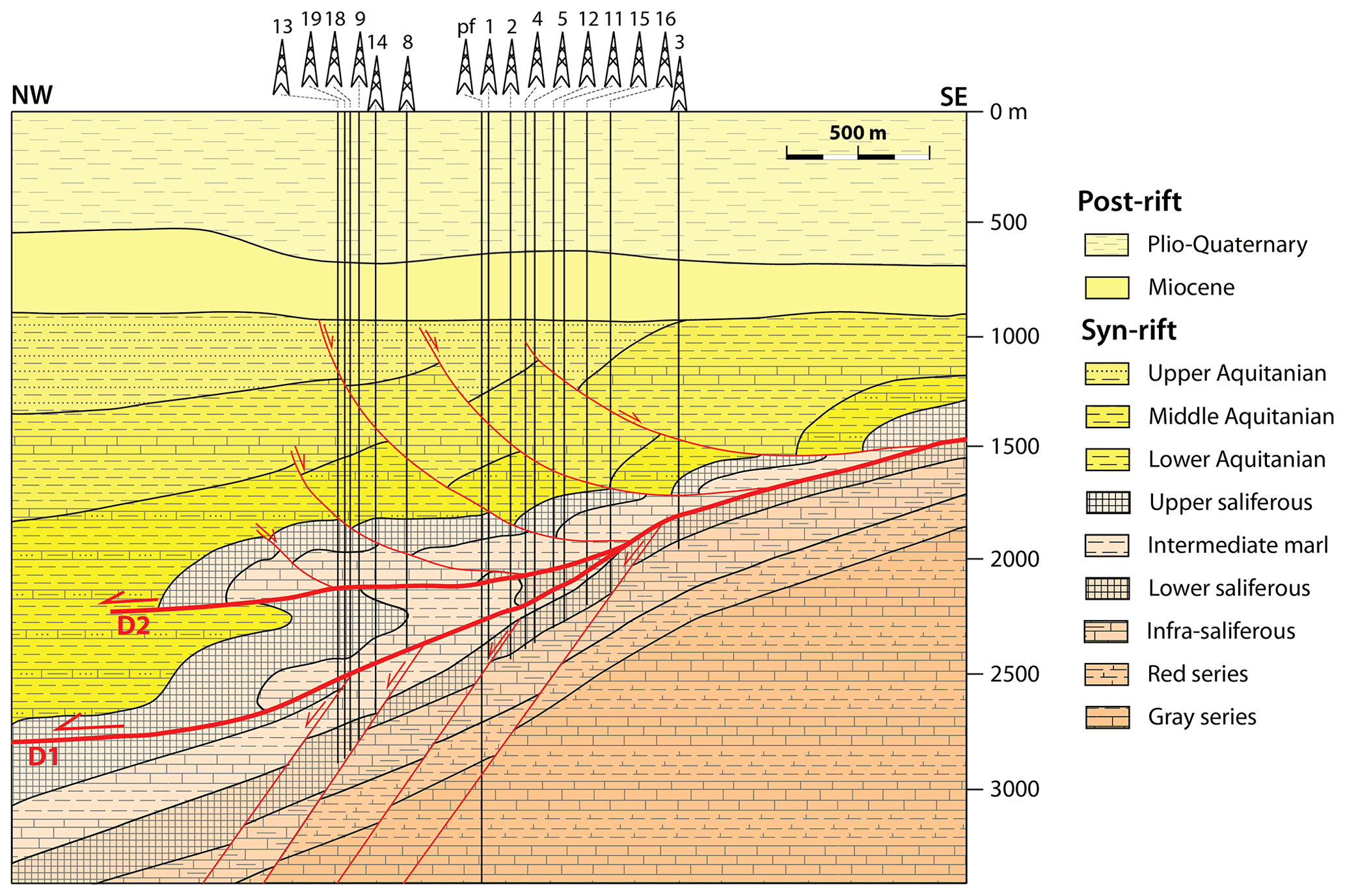
Figure 1Geological structural scheme of area under study crossing the numbered wells (Derrick symbols at the surface, pf is for Pierrefeu well) at Vauvert (from Valette and Benedicto, 1995). D1 and D2 represent the two decollements (thrust fault) affecting the salt layers.
2.2 Salt extraction
The deep salt deposit of Vauvert was discovered during the 1952–1962 oil survey conducted by ELF (Valette, 1991). Since 1972, the company KemOne (previously ELF ATOCHEM-Saline de Vauvert) has been extracting the salt from deep caverns (1500–3000 m) in the form of a solution saturated in salt, i.e., the brine. The brine is then carried out to Fos-sur-Mer (70 km southeast of Vauvert) to be used in the chemical industry producing chlorine and caustic soda. The brine is recovered using two or three wells (doublets or triplets) hydraulically connected in the salt layer by initial or induced fracturing of the medium. Among the currently drilled wells (about 47), only 12 are still extracting brine, two are being vented (to release overpressure at the well head due to salt creeping), and the other ones are sealed. For the active sets, water is injected into one well at a pressure of 9.5 MPa, while the second extracts the brine at 0.2 MPa. The underground circulation of fluid is allowed by the induced fracturing created to connect the wells. Once the salt concentration in the brine reaches a minimum threshold (the extracted water does not contain enough salt to be exploited), doublets are abandoned and sealed. This implies an increase in pressure from the bottom to the top of the wells, due to salt creeping. For security reasons, the pressure needs to be released by opening the wells, allowing brine to flow and salt to creep until lithostatic equilibrium. In 2019, up to 1 × 10⁶ t of brine were extracted from about four active doublets (plus two as backup doublets).
3.1 A wide network
The monitoring of subsidence above salt extraction in Vauvert has been performed since 1996 by IGN using leveling surveys along with a collection of InSAR data acquired by various satellite missions (ERS, ENVISAT, SENTINEL; Fig. 2a). Raucoules et al. (2003) first characterized the subsidence using from ERS-1 and ERS-2 images. Only vertical velocity could be estimated, leading to a maximum subsidence rate of 22 mm yr−1. A permanent GNSS station was installed in November 2015 followed in October 2016 by three new permanent stations. Figure 2a represents the temporal coverage of all geodetic techniques employed to monitor the site. In this study, we only use Sentinel images because of their general features, including medium resolution, high revisit time (6 d), intermediate acquisition band (C-band), and easily accessible data. Hence, we derive an annual deformation velocity from InSAR analysis (Sentinel-1a/b images) and leveling surveys measuring between 2015 to 2017 and permanent GPS data (2015–2019). Figure 2b shows the spatial coverage of leveling surveys and GPS networks used in this study.

Figure 2(a) Temporal coverage of geodetic networks monitoring the site. (b) Spatial coverage of GNSS and leveling network of the salt exploitation in Vauvert. Well heads are represented by red circles, permanent GNSS is represented by yellow inverted triangles, and leveling benchmarks are identified by blue crosses. The red line indicates the profile A–B for leveling data represented in Fig. 3a. The blue areas represent the extent of Vauvert and Beauvoisin cities, while the black line defines the extent of the KemOne company. The background map is extracted from IGN SCAN 1:25 000 (© IGN).
3.2 Leveling surveys
The height differences between two points of the network were determined by direct geodetic leveling (double run) carried out using an electronic level LEICA WILD NA3003, on a round trip pattern. This instrument has an accuracy of 0.1 mm, and the standard deviation of measurements for 1 km of round-trip leveling is 0.4 mm (manufacturer data). IGN has conducted the processing using the Geolab least squares adjustment program (version 2001.9.20.0). This type of tool makes it possible to provide for each of the points an elevation as well as an indicator of the accuracy of the result. The accuracy is estimated from the observations and not only from manufacturer nominal features. The mean data uncertainties from the 2019 survey reaches 1.34 mm. Figure 3 illustrates the leveling measurements performed between 1996 and 2018 along the profile A–B in Fig. 2b. These surveys started in 1996 with 39 leveling benchmarks; new ones (almost 100) were added progressively to densify the network and some needed to be replaced (destruction, shift, instability of a benchmark). Since 2006, about 137 benchmarks have been measured yearly (except in 2013 and 2015). The velocity associated with the subsidence of the marker highlighted by the red rectangle in Fig. 3 is estimated by the ratio of the vertical displacement over the time interval between two measurements (i.e., 1 or 2 years). The vertical velocity is variable in time (Fig. 3b), with a strong increase in the subsidence rate between 2002 and 2003; since then the subsidence rate has been relatively steady around 26 mm yr−1 in the center of the subsidence area (red line in Fig. 3b).
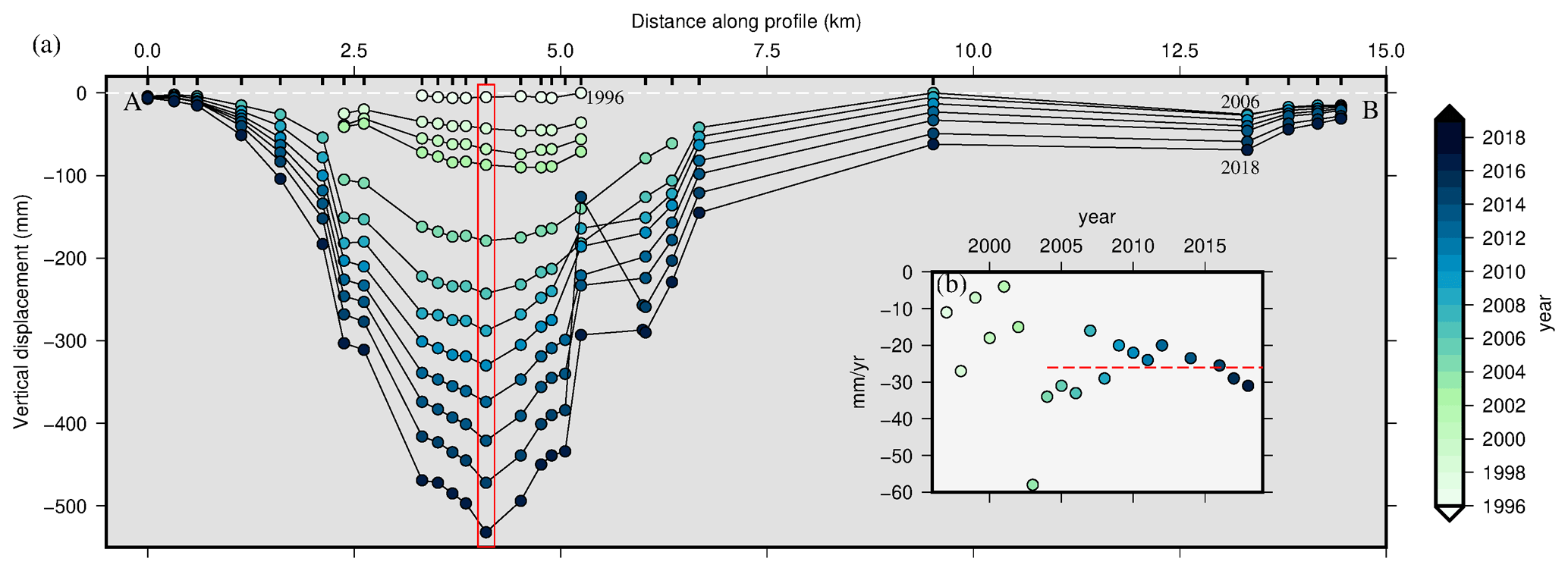
Figure 3(a) Leveling data along the A–B profile (red line in Fig. 2b) performed by IGN from 1996 to 2018 (color scale). Data are displayed every 2 years for ease of reading. (b) Deformation velocity associated with the marker with the largest subsidence (red rectangle in a). The velocity is given for each year, using the same color scale as in (a). The red dashed line represents the mean velocity of vertical displacement observed from 2004 to 2018.
3.3 InSAR data
Radar images from Sentinel constellation imaging satellites (Sentinel-1a and Sentinel-1b) are recorded on the C-band frequency (similarly to Envisat) and present a short temporal redundancy of about 6 d, limiting the temporal decorrelation. The perpendicular baseline between the images is very short, a few tens of meters, which also limits the spatial decorrelation. Sentinel constellation images have a swath of 250 km wide and a resolution of 5 m×20 m, in both ascending and descending geometries. InSAR accuracy is strongly dependent on several factors, including SAR data and PS availability, artificial corner reflectors, the ambiguous nature of the observation, line-of-sight deformation measurements, and deformation tilt and trends (Crosetto et al., 2016). The velocity along the line of sight can be measured with an accuracy of a few millimeters. In this study, we used 101 ascending and 66 descending images between 18 April 2015 to 3 December 2017 to produce a mean displacement velocity field and time series. Ascending geometry is characterized by a flight direction with respect to the north of 103.96 and an incidence angle of 32.93∘, while descending geometry is defined by a flight direction with respect to the north of 256.01∘ and an incidence angle of 36.98∘. We develop a PS–InSAR processing chain based on existing algorithms (e.g., SNAP, StaMPS). The preparation of single-look complex (SLC) images and the creation of the interferograms are carried out with the software SNAP from the European Space Agency (ESA). Precise orbits provided by ESA (DORIS) are applied to finely process the geometric positioning of the image portions (bursts). Master image are chosen so that the time and the perpendicular baseline are optimized: images of 26 November 2016 for the descending geometry and 27 November 2016 for the ascending geometry. The two SLC images (master image and slave image) of the same subdomain are co-registered using the orbits of the two products and the 90 m resolution digital terrain model, Shuttle Radar Topography Mission (SRTM) (Farr and Kobrick, 2000; Farr et al., 2007). With known satellite orbits, a correction of the effect of the Earth's curvature on the phase is applied. The geodetic reference system is defined by the satellite orbit reference system (WGS84, the reference system used by all space SAR systems). The topographic phase is removed from the interferogram using SRTM. In addition, the information about the altitude is available for each PS.
Once the interferograms are created under SNAP, they are imported and processed with StaMPS processing software (Hooper et al., 2004). The pixels are selected according to an amplitude dispersion criterion, and a maximum proportion of “false” PSs is set to 20 %. Digital elevation model (DEM), master atmosphere, orbit, and look angle error are estimated and removed. Finally, the fringes of the resulting phase are unwrapped (Fig. 4a and b for ascending and descending geometries, respectively). From the unwrapped interferograms, we have relative displacements in time associated with each PS. Then, by applying a linear regression on relative displacements from each PS, we get position time series. A previous study (Raucoules et al., 2003) and leveling measurements have shown that velocity can be considered constant with time. So, using a linear regression over the 2-year time period of this study, this leads to velocities. Associated uncertainties are finally obtained using the standard deviation of PS velocities. The maximum subsidence rate is 24 mm yr−1. The associated uncertainties are lower than 4.5 mm yr−1 for the ascending track and 2.9 mm yr−1 for the descending track with mean values of 1.2 and 0.6 mm yr−1, respectively (Fig. 4c and d).
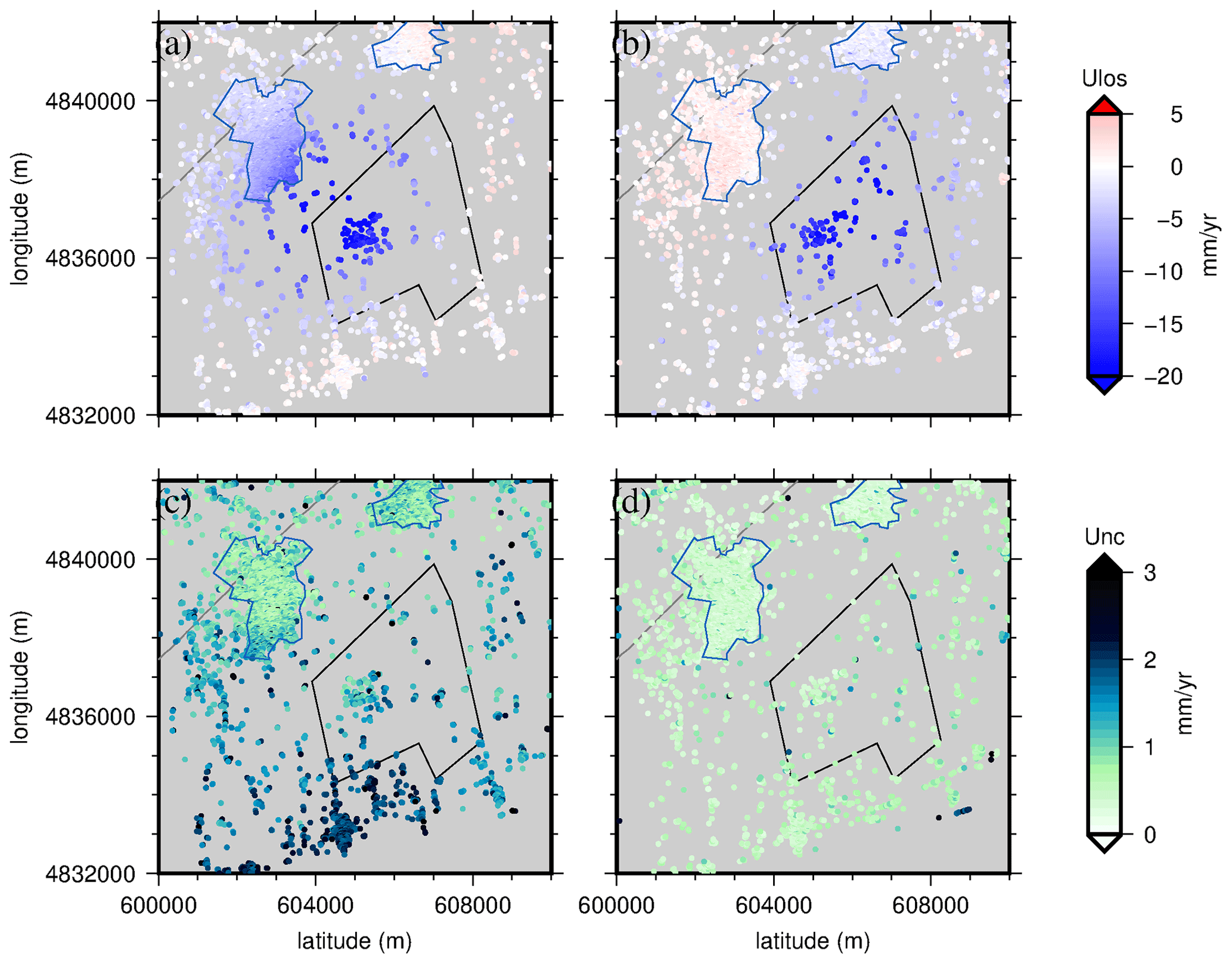
Figure 4Mean velocity in LOS direction in (a) ascending and (b) descending interferograms over the area of interest and their associated uncertainties (c) and (d), respectively. Ascending geometry is characterized by a flight direction with respect to the north of 103.96∘ and an incidence angle of 32.93∘. Descending geometry is defined by a flight direction with respect to the north of 256.01∘ and an incidence angle of 36.98∘. The polygons represent the extent of Vauvert and Beauvoisin cities (blue polygons) and the KemOne company area (black polygons; see Fig. 2b).
3.4 Continuous GNSS
Four permanent GNSS stations (Fig. 2) sampling at 30 s were set up, respectively, in November 2015 (VAUV station) and October 2016 (VAU1, VAU2, and VAU3 stations) to characterize more accurately and in three dimensions the variations in the deformation and its spatial extension. The measure of the GNSS position is a three-component value generally given with a daily accuracy of 1 mm (Hager et al., 1991) with respect to a reference frame called the International Terrestrial Reference Frame (ITRF). The processing of coordinates and velocities is done using the Gamit-Globk v10.7 software (Herring et al., 2015). We use the well-documented three-step approach and take advantage of the “realistic sigma” algorithm to estimate the uncertainties (see Reilinger et al., 2006, for details). We include in the processing 26 continuous stable reference stations located within a 150 km radius of the Vauvert sites. These sites belong to the permanent RGP, RENAG (RESIF-RENAG French national Geodetic Network; RESIF – Réseau Sismologique et Géodésique Français), or ORPHEON networks and allow us to define a stable regional reference frame by minimizing the velocities of these 26 sites. The resulting station position time series for the north, east, and vertical components are free of any regional tectonic displacement and show only local processes.
Figure 5a–c plot the time series of the three components of VAU3 station (Fig. 2) from 2016 to 2019. Once the seasonal effects are removed, the trends are quasi-linear in time for all three components. We represent the velocities of the sites near the exploitation with respect to a local stable reference frame in Fig. 5d and e (i.e., all the velocities outside of the mapped area can be considered as equal to ∼0 mm yr−1). The horizontal velocities (Fig. 5d) measured at each station show a significant displacement toward the center of the exploitation. The vertical velocity (Fig. 5e) indicates a maximum subsidence of −25.8 ± 0.2 mm yr−1 but with greater magnitudes at the edges of the bowl (−13.8 ± 0.7 mm yr−1 at VAU3 and −17.9 ± 0.7 mm yr−1 at VAU2) than those previously measured (Raucoules et al., 2003).

Figure 5Time series of the three components (a) north, (b) east, and (c) vertical, measured at station VAU3 from 2016 to the end of 2019. (d) Map of horizontal velocities and well locations. (e) Vertical velocities, downward being subsidence. The polygons represent the extent of Vauvert and Beauvoisin cities (blue) and the KemOne company area (black; see Fig. 2b).
4.1 Methodology
4.1.1 General remarks on the combination
Terrestrial (e.g., leveling, inclinometry) and satellite-based (e.g., GNSS, InSAR) geodetic measurements are complementary in terms of accuracy and spatial or temporal resolution, from slow ground displacement monitoring (e.g., Hastaoglu et al., 2017) to rapid surface changes (e.g., Peltier et al., 2017). Many attempts to combine these geodetic measurements have been described and published recently (e.g., Catalão et al., 2009; Burdack, 2013; Lu et al., 2015), to overcome the limitations and inadequacies of the different techniques in difficult contexts, when taken separately (e.g., Karila et al., 2013; Abidin et al., 2015; Fuhrmann et al., 2015; Comerci and Vittori, 2019). The combination of several geodetic measurement techniques aims to improve the knowledge of the ground motion by overcoming or at least mitigating each technique's shortcomings with the other. In this study, we propose a methodology to combine InSAR and leveling data to produce a 3-D velocity field associated with the salt extraction of Vauvert (Doucet, 2018). Unlike GNSS and leveling data that are precisely constrained on the Terrestrial Reference Frame (TRF), InSAR is a relative measurement in space and time, with no precise datum. So, InSAR data have to be adjusted, constrained, or tied-in to a TRF. The number of GNSS stations and, mostly, the temporal coverage of time series are not statistically representative of the deformation for being appropriately incorporated in the combination (only one out of four stations continuously measured the deformation between 2015 and 2017). Indeed the combination is based on the following assumptions.
-
Reference frames adjustment. Horizontal absolute positioning, at the time of the processing, was not sufficiently constrained, so obvious PSs along roads (especially crossing roads) were used to obtain latitude and longitude shifts. In order to compare InSAR to leveling and GNSS data, we first correct the horizontal position of PS points using the mean value of all horizontal shifts manually detected on the interferograms. Second, we adjust the reference system of interferograms using a two-dimensional linear ramp (Lundgren et al., 2009; Hammond et al., 2010) based on the calculation of differences between velocities at 26 GNSS stations and PS data points near these stations.
-
Sufficient measurement density. We assume that the density of reliable permanent scatterers is sufficient for the considered area in both ascending and descending InSAR geometry results. Besides, we consider that leveling and InSAR measurements are dense enough to be statistically representative of the deformation. Hence their distribution can be interpolated using kriging methods (ordinary and weighted regression).
-
Satellite measurement geometry. We assume that for the area of interest, flight directions of the satellite with respect to the north (β) are symmetrical with respect to the north–south axis ( and with respect to the north, leading to identical look angles for both geometries). The angles of incidence between the satellite and the permanent reflectors at the surface are considered nearly identical in the ascending and descending geometry acquisition ( and ). This allows us to estimate the east component of the deformation along with a near-vertical component.
-
Radial deformation. The surface deformation observed in the area of interest shows a quasi-symmetrical bowl of subsidence (Raucoules et al., 2003). We hence make the assumption that this symmetry affects all components of the displacement, leading to the estimation of the north component with an acceptable accuracy.
Although these hypotheses may be false for other cases, in the case of Vauvert, and given the previous available information from InSAR (Raucoules et al., 2003) and leveling, they allow us to compute the first-order three-dimensional velocity field associated with the salt extraction. We review and comment on these choices in the discussion regarding the results of both the combination and the inversion. Figure 6 represents the general algorithm of our two-step methodology to combine interferograms and leveling data involving (1) a 3-D geometrical estimation and (2) a weighted regression kriging.
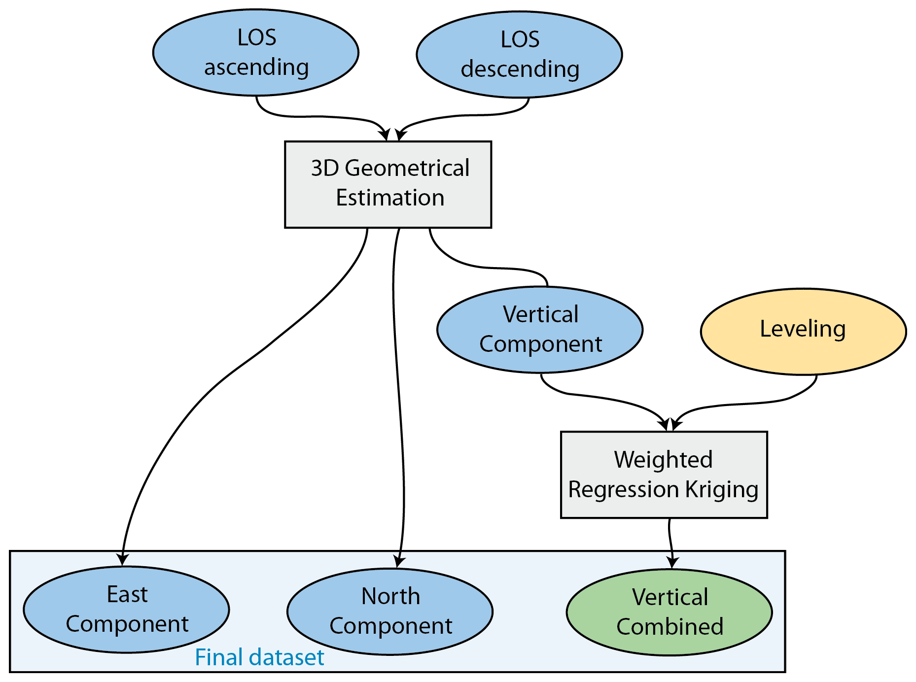
Figure 6Algorithm of the two-step methodology developed to combine deformation velocities estimated from interferograms and leveling surveys. (1) Three-dimensional geometrical estimation is performed to derive east, north, and vertical components from ascending and descending InSAR geometries. (2) The vertical component and leveling data are combined using a weighted regression-kriging technique.
4.1.2 Step 1: 3-D geometrical estimation
The first step of the approach consists of interpolating the ascending and descending InSAR data by ordinary kriging, in order to densify the spatial distribution of PS points, so that they can be virtually colocated with leveling benchmarks. The kriging interpolation models the best linear unbiased prediction of the intermediate values by a Gaussian variogram model (driven by prior covariances). The number of data points, position, and uncertainties are considered in the interpolation, leading to interpolated values of the data distribution along with uncertainties (kriging variance that accounts for the data uncertainties). By applying a weighting function based on the correlation between the data and the distance between them, the kriging method allows canceling the effect of a high-density area, typically cities, where PSs are more concentrated than elsewhere, notably poorly anthropized areas where the number of data points can be low. We use ordinary kriging to densify the spatial distribution of PSs (Cressie, 1988; Yamamoto, 2005; Daya and Bejari, 2015; Ligas and Kulczycki, 2015). The associated uncertainties are given by ordinary kriging as the weighted variance of the interpolated distribution of PSs.
The velocity vPS, measured at each point on the ground, corresponds to the component along the radar line of sight (LOS) of the deformation. It contains portions of all three dimensions of the velocity, depending on the geometry of the acquisition and the angle between the vertical and the measured point, such as
where v is the three-dimensional vector of the velocity and s is the unit vector pointing from the ground towards the satellite. This unit vector is defined by the incidence angle (Θ) and by the flight direction with respect to the north (β) associated with each geometry of acquisition.
Using assumption 3 from Sect. 4.1.1 leads to components of the unit vectors for ascending and descending geometries such as , , and . Because the maximum deformation in the area of interest is on the order of 10 to 20 mm yr−1 (for the north and vertical components), this assumption induces errors ranging from 0.1 to 0.8 mm yr−1, which are 1 order of magnitude lower than data uncertainties. Using the components of the unit vectors for ascending and descending geometries, we can deduce the relation to estimate the east and a near-vertical component of the velocity. The near-vertical component vnu is used to defined the complex geometry of the subsidence bowl, so that its shape is given by the iso-contour vnu=0 and its center is determined by the junction of the maximum subsidence () and zero velocity along the east–west direction. To extract the north component we assume that the horizontal component of the velocity is radial and pointing towards the center of subsidence. Using an east–west profile crossing the center of subsidence, we project the horizontal component of the velocity of crossed points (i.e., pure east velocities) onto this profile to deduce the north component. We rotate the profile around the center of subsidence and adapt its length to the bowl size, to get the horizontal component (including ve and vn). When the profile is oriented along the north–south axis, pure vn is estimated.
The 3-D components of the velocity field derived from InSAR can be defined as
where vh is the velocity in the horizontal plane of a point p, such as
where α is the angle between the E–W axis and the azimuth of the profile relative to the center of the bowl. vhe and vhw correspond to the velocities projected along the profile (of zero velocity), crossing the center of subsidence. This method allows us to estimate the north component from a complex shape of subsidence bowl, considering a radial surface deformation. From these relations, we produce the three-dimensional velocity field associated with the extraction of salt in Vauvert.
4.1.3 Step 2: weighted regression kriging
In the second step of our combination approach, we use a regression-kriging method (e.g., Hengl et al., 2007) to refine the vertical velocity field in the areas where leveling data are available. Indeed, leveling surveys provide accurate measurements of the vertical velocity field but only on a finite number of points (120). Regression kriging is a spatial prediction technique that combines a regression of the dependent variable (dual geometry InSAR in our case) on auxiliary variables (leveling data in our case, but it could also be GNSS if they were consistent in time) with kriging of the regression residuals. It is mathematically equivalent to kriging with external drift, where auxiliary predictors (leveling) are used directly to solve the kriging weights (Pebesma, 2006). Also, leveling benchmarks are only distributed along linear paths, making the use of co-kriging inappropriate to combine InSAR and leveling data on a spatial grid. Instead, regression kriging uses regression on auxiliary information and then uses simple kriging with known mean (0) to interpolate the residuals from the regression model (Hengl et al., 2004). This method allows us to make predictions by modeling the relationships between the target and one or more auxiliary variables (the predictor(s)) at common sampling locations. In this study, we use the generic framework developed by Hengl et al. (2004) for spatial prediction of the vertical velocity field. We sample the vertical velocity field from InSAR data (target data) at the leveling benchmarks' location (auxiliary data). Then, a linear regression of a target variable (vu) on predictors (leveling) is applied with a kriging of the residuals of the prediction. Finally, we estimate a reliability index at each point of the grid, taking into account the uncertainties of each technique and the uncertainty associated with the interpolations.
On Fig. 7a to c we represent east, north, and vertical components of the velocity resulting from the data combination, along with their associated uncertainties (Fig. 7d to f). The incorporation of leveling data in the combination allowed refining the vertical component of the velocity measured from dual geometry InSAR. The deformation induced by the salt exploitation in Vauvert is characterized by both horizontal and vertical displacements. Compared to Raucoules et al. (2003), the combined dataset (along with GNSS velocities) allows us to identify significant horizontal displacements. East and north components of the velocity field indicate a maximum subsidence rate towards the center of the exploitation (Parrapon site, black dots in Fig. 7) of about 18 mm yr−1 (Fig. 7a and b). The maximum vertical velocity reaches 24 mm yr−1 (Fig. 7c) and is located above the salt exploitation of Vauvert. The subsidence affects a large area in a radius of about 3 km from the center of the exploitation (black dots in Fig. 7).
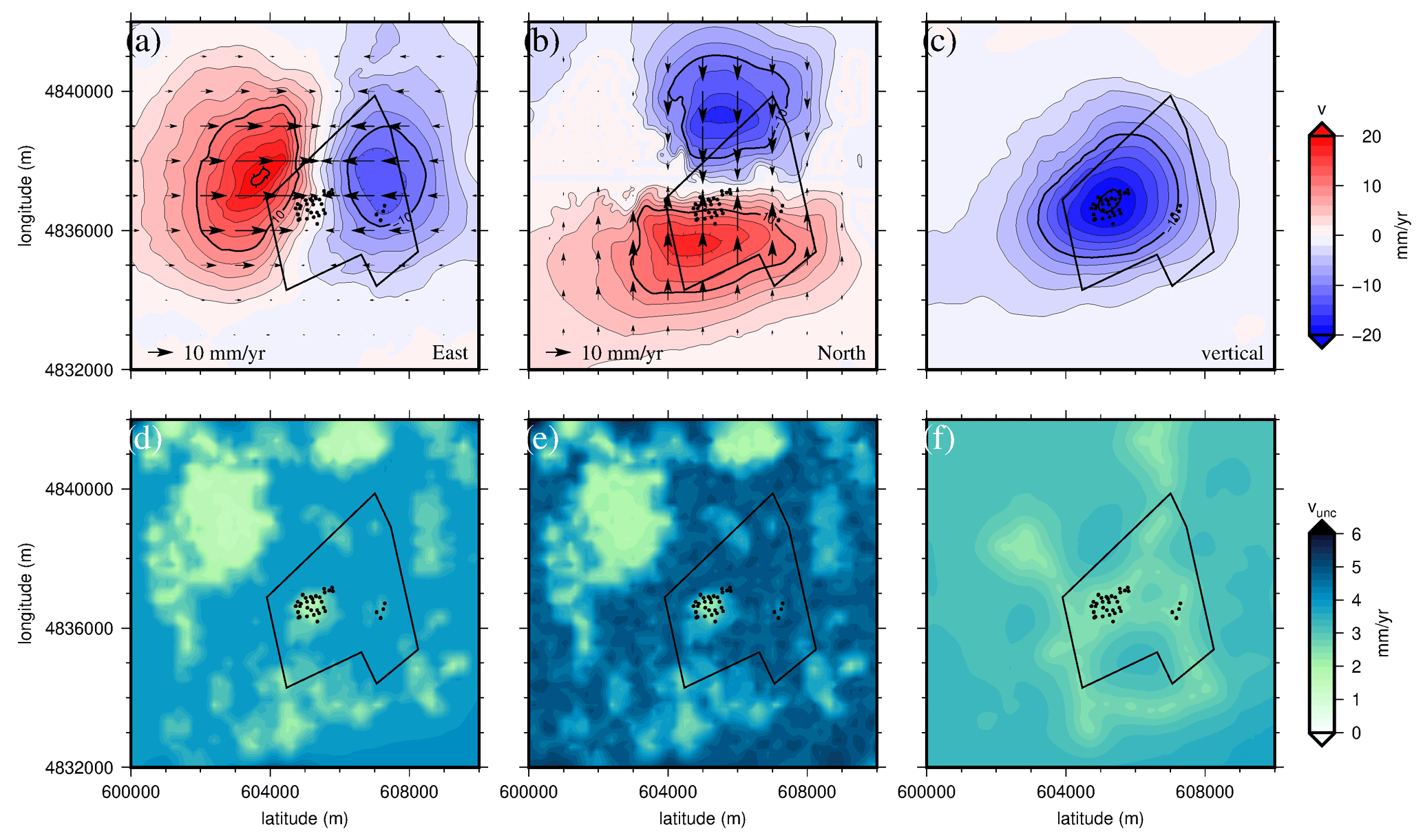
Figure 7The three components (east, north, and vertical) of the velocity field calculated using the two-step methodology described in this section (a–c) and their associated uncertainties (d–f). Black arrows indicate the horizontal velocities on (a) and (b). The black dots show the well locations. The black polygon represents the KemOne company area (see Fig. 2b).
4.2 Comparison with GNSS velocity field
The combination of InSAR ascending and descending data with leveling data produces a 3-D velocity field measuring the deformation above the salt exploitation of Vauvert. The vertical velocity computed through this combination is fairly similar to the one estimated by Raucoules et al. (2003). Differences may notably stem from both the period of interest and the incorporation of leveling data (as opposed to stand-alone InSAR). In Fig. 8, we compare the three components of the velocity field derived from the dual InSAR geometry–leveling combined set to their GNSS counterparts. It shall be noted that the GNSS uncertainties are lower than 0.8 mm yr−1, so not significant enough to be represented in the figure. Even though this comparison is only indicative due to observation times not perfectly matching each other, one may notice, however, that on all four points the combined set correctly matches the GNSS in both east and north (with the GNSS circles located within the uncertainty bars), whereas there is no matching in the vertical for two points (VAU2 and VAUV). The latter inconsistency is all the less surprising as VAUV is located close to the subsidence bowl center (where subsidence magnitude is changing faster) and VAU2 is located close to the north edge of the bowl (the subsidence bowl has migrated northward due to extraction wells shifting accordingly). However, even though the combined set and the GNSS are fairly consistent with each other, it shall be emphasized that they could not perfectly match each other due to their different time coverages of an area very sensitive to the location of the extraction wells (which were shifted in time).
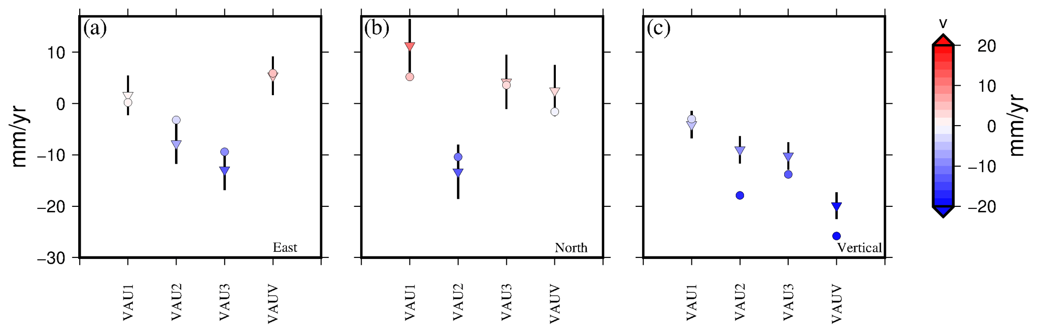
Figure 8Three components of the velocity from GNSS and the Dual InSAR geometry–leveling combined dataset observed at GNSS locations (VAU1, VAU2, VAU3, VAUV; see Fig. 2). Inverted triangles represent the (a) east, (b) north, and (c) vertical components of the velocity from the combined dataset, the vertical bars indicate the associated uncertainties, and the circles stand for the GNSS dataset.
5.1 Forward models
The salt formation lies between 1500 and 3000 m deep in sheet-like layers dipping at 30 ± 5∘ induced by the presence of normal faults and two decollements D1 and D2 (Valette and Benedicto, 1995; Fig. 1). Previous studies (Maisons et al., 2006; Raucoules et al., 2003, 2004) have highlighted a quasi-perfect axi-symmetrical bowl of subsidence in Vauvert originating from the exploitation of this salt formation. In this study, the combined dataset (Fig. 7) shows a consistent vertical signal but also provides horizontal displacements. Hence, we consider four analytical models of the salt layer of increased complexity to best explain the velocity field measured by the geodetic dataset: a single point source, a rectangular plane, and two collections of 21 and 28 square planes. In the case of Vauvert's exploitation, using elastic models allows us to model the surface displacements induced by the brine extraction but also possibly by salt creep. However salt creep is reduced to shear on planes without any further rheological considerations.
First, we use a simple Mogi source (Mogi, 1958) to model the volume variations in the salt layers at depth (model 1). It considers a spherical source embedded in a semi-infinite uniform elastic body. The source is defined by four variables: its Cartesian coordinates () and its volume variation (ΔV). The point source being the less representative model of the salt layers, we do not constrain it with geological information and keep the four variables of the source free during the inversion.
Second, we consider a 2-D plane of dislocation (model 2) with parameters (position, depth, dimensions, dip, azimuth) set according to the salt layer properties for a more realistic model. The forward model uses three-dimensional, elastic dislocation theory in a homogeneous half space (Okada, 1992). The source is a patch, characterized by its position, dip, azimuth, length, width, depth, and dislocation type (strike, dip, or tensile). The plane is centered on the salt exploitation at a depth of −2250 m and covers the allochthonous saliferous unity, up to La Galine's boreholes (orange rectangle in Fig. 9). The plane has a strike dip of N 50∘ E, 30∘ NW with depths ranging from 1500 to 3000 m (the top of the plane, at 1500 m, is identified with the double orange line in Fig. 9). Most of the exploitation wells (red dots in Fig. 9) are located at the Parrapon site. La Galine's wells are no longer active (two wells), and brine is extracted only to release pressure. It means a very low brine production during the time considered. All but the dislocation parameters are fixed using available geological information, such as the inversion process seeking only three parameters. Hence, Green's functions describing the analytical solution for the surface displacements v (Okada, 1992) are linear with the dislocation parameters:
where is the dislocation type j (strike 1, dip 2, or tensile 3) associated with each plane i and is three-dimensional vectors between the point at the surface with the displacement v and the dislocation at depth.
The combined velocity field suggests a more complex source deformation and a single source may not be sufficient to explain the surface subsidence. Thus, we discretize the salt layer into several dislocation patches, to increase the degrees of freedom for the sources to model the surface deformation. The single rectangular plane is subdivided into 21 square planes (model 3) of 1 km side. The orientation is the same for the 21 patches and locations and depths are set accordingly to the salt layer characteristics, all these parameters are fixed (Fig. 9). In this model, each plane has its own independent strike-slip, dip-slip, and tensile components, such that both the rapid depletion at the vicinity of the exploiting wells and the creeping deformation in the salt layer can be considered. We consider 63 free dislocation parameters to be retrieved by inverting the combined dataset, fixing all other parameters of the planes (positions, orientations, dimensions).
For model 4, we add a fourth row of planes (dashed orange line in Fig. 9) to study whether boundary effects in model 3 exist. This last row of planes is set at 3250 m depth (bottom of planes is at 3500 m), and its extension at the surface reaches the limits of Vauvert city. Similarly to model 3, only dislocation parameters are optimized, leading to 84 free parameters to be retrieved.
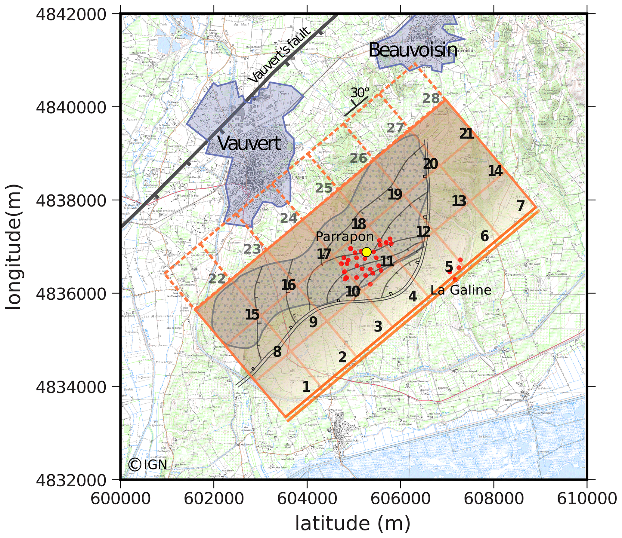
Figure 9Representations of the dislocation planes (numbering from 1 to 28) are displayed in shaded orange modeling the salt layer (darker shading for deeper planes), along with the currently known boreholes (red dots). The decollements are represented by the double line and listric faults by black lines beneath the site of salt exploitation in Vauvert (France). The allochthonous saliferous unity is represented by the gray dotted area. The limits of Vauvert and Beauvoisin cities are represented by blue areas, and the Vauvert normal fault is displayed using black lines (modified from Valette and Benedicto, 1995). The blue polygons represent the extent of Vauvert and Beauvoisin cities (see Fig. 2b). The background map is extracted from IGN SCAN 1:25 000 (© IGN).
5.2 Inversion strategy
For model 1, the position of the source is sought in the 10 km×10 km area defined by Figs. 2 and 9. Source depth can vary between 0 and 5000 m depth, and volume variation is investigated between 0 and −1.5 × 10⁶ m3. For models 2 to 4, the dislocations parameters (strike-slip, dip-slip, and opening) are set free to vary between −1 and 1 m throughout the inversion process. For the multi-source models (3 and 4), no smoothing conditions are considered between planes. Initialized with no a priori information, a first modeled dataset is produced which is compared to the observations. We choose to build the functional as the weighted Euclidian norm of the residual vector D between observed and modeled dataset:
where Σ is the data covariance matrix associated with each point of the dataset and T denotes the transpose of the residual vector. Through this formulation of the functional, we consider the resolution of the measurements: for highly uncertain data, their covariance matrix is large compared to the data values, leading to small values of J. This functional needs to be lower than the data uncertainties or reaches a minimum value for the optimization to be completed. This linear problem (Eq. 7) is solved using an optimization algorithm allowing us to process problems with non-linear relations. By doing so, we can easily switch to a different forward model, including more complex and realistic physics without implementing a new optimization approach. Our optimization process is based on a recursive algorithm defining a multi-criteria global optimization, varying not only the parameters of the model but also the initial guesses (Ivorra and Mohammadi, 2007; Mohammadi and Pironneau, 2009). This allows us to ensure that a given set of optimal model parameters realizes the global minimum of the functional.
To determine the model parameter uncertainties, we implement the approach developed by Mohammadi (2016) using backward uncertainty propagation. This approach is based on the introduction of directional quantile-based extreme scenarios knowing the probability density function of the target data. By doing so, we avoid computing numerous scenarios of data perturbation to generate the probability density function (PDF) of a functional J. Instead, we use the sensitivity of the functional with respect to the data and explore only the optimal region given by the optimization to identify two directional extreme sets of data. Two datasets are obtained by perturbating observed data vi knowing the associated data uncertainty σi along the direction given by residual value between optimal and observed data (the fractional term is equal to 1 or −1).
These two datasets are then inverted to obtain two sets of optimal parameters, corresponding to the extreme values each parameter can take given the uncertainties on the observations and the residuals. The maximum and minimum deviations for the optimal parameter set are hence given by these two extreme scenarios.
5.3 Results of the inversion
5.3.1 Model comparison
We compute the difference between the observations and the model to obtain the residual values. These residuals are used with the data uncertainties to estimate how the model fits the dataset using the normalized rms (NRMS) (McCaffrey, 2005):
where N is the number of observations, r is the residual, and σ is the data uncertainty. This unitless level indicates whether the model fits the observations with respect to data uncertainties and should be close to 1. Besides, we can also compute the weighted rms (WRMS) from McCaffrey (2005), which gives an estimation of the a posteriori weighted scatter in the fit.
Table 1 present the residuals, NRMS and WRMS for the east, north, and vertical components of the velocity field for each model. The total NRMS and WRMS are also given in Table 1.
Table 1Inversion results for the four models described in Sect. 5.1. Residual values (columns 2–4), NRMS (columns 5, 7, 9), and WRMS (columns 6, 8, 10) are indicated for each component of the velocity field and for the whole dataset (columns 11–12).
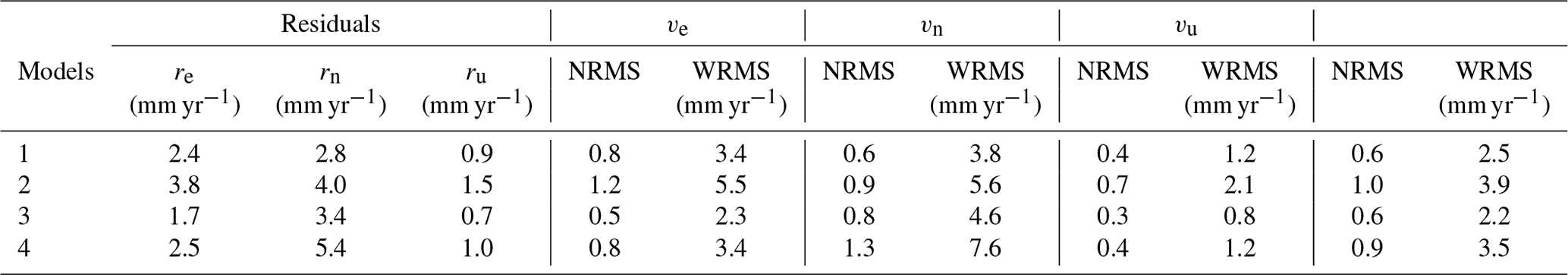
Considering model 1, the inversion leads to an optimal point source located 1971 m deep at the north end of the Parrapon site, associated with a volume change of −390 099 m3 (0.8 × 10⁶ t of brine). The real mass of extracted salt of about 1 × 10⁶ t of brine every year at 2 km depth (1.0 × 10⁶ t in 2015, 0.93 × 10⁶ t in 2016, and 1.08 × 10⁶ t in 2017) suggests that this model slightly underestimates the volume loss. The projected location at the surface of this source matches the center of the dislocation plane of model 2. The depth of the point source is shallower than expected since it corresponds to the top of the salt layer. Furthermore, if the vertical component of the deformation observed in Vauvert can be reasonably modeled by a single point source, the horizontal components are underestimated. Hence, the horizontal displacements can not be solely explained by the centripetal displacements induced by the subsidence.
The 2-D dislocation plane of model 2 provides a solution with high residuals (Table 1) and low fit to the observations for both horizontal and vertical velocities. The volume change of this model of −329 000 m3 (0.7 × 10⁶ t of brine) also underestimates the real discharge. One can postulate that with the salt extraction located roughly at the center of the salt layer horizontal extension, the salt flow should induce horizontal displacements toward the well locations; hence a single plane cannot fit the observed deformation.
To check this hypothesis, we discretize the salt layer into several planes of dislocation. In doing so, we increase the degrees of freedom of the sources to model the surface deformation. Model 3 presents the lowest values of residuals, NRMS, and WRMS for the east and vertical components, suggesting that horizontal displacements at depth are needed to explain the observations. However, the north component remains partly unexplained, certainly due to the high uncertainties related to the method we use to extract the north component from the InSAR signal. We estimate a volume change of −556 000 m3 corresponding to a mass of 1.21 × 10⁶ t per year of extracted salt, which slightly overestimates the real mass of salt.
Increasing the number of planes to 28 in the model by adding a fourth row at greater depth does not improve the residuals nor the fit to the horizontal components. Besides, the volume change associated with this model reaches −751 000 m3 (1.6 × 10⁶ t of brine), largely overestimating the real volume loss.
The geometry of 21 dislocation planes model, the residuals (NRMS and WRMS), the estimated volume loss, and the agreement with the geological setting of the salt layers (Fig. 1) suggest that it is the best model. We hereafter describe the results of the inversion for this model.
5.3.2 Parameters and resolution analysis
The inversion leads to a distribution of strike-slip, dip-slip, and tensile dislocations associated with each plane of the model (black dots in Fig. 10a to c). We estimate the upper and lower admissible value associated (at 2σ) with each dislocation parameter, using the directional extreme scenarios as previously described. The blue and red dots in Fig. 10a to c stand for the two extreme scenarios (v+ and v−, respectively). In both scenarios, the distributions remain close to the optimal solution. By calculating the difference between the optimal solution and each scenario, we compute the range of confidence for each parameter. These confidence intervals are on the order of several centimeters (up to 10 cm for the largest intervals). For instance, the plane containing most of the exploitation wells (plane 11) closes (tensile dislocation) at a value between 30.9 and 38.6 cm at 2σ. This means that the solution obtained from the inversion is robust and is the best we can get with respect to the data and their uncertainties. If confidence intervals include zero deformation (with respect to parameter uncertainties), then we can say that the determined displacement is not significant at 2σ.
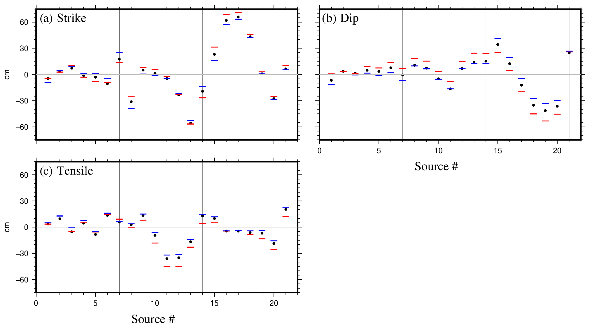
Figure 10Interval of confidence (2σ) for the dislocation parameters of the 21 sources: (a) strike slip, (b) dip-slip, and (c) tensile. The black dots represent the optimal value of the parameter; red and blue are associated with the two extreme scenarios (v+ and v−, respectively) obtained using the backward uncertainty propagation previously described. The black lines on the graphs separate the sources contained in the three lines that composed the model. The gray line indicates zero deformation of the plane.
We represent the distribution of dislocation values associated with each plane in Fig. 11. The planes where the displacement is not significant are colored in gray. From Fig. 11a, b, and d, one can observe that most of the slip motion occurs on the deepest planes. The strike-slip motions range from −55.8 to 65.8 cm, while dip-slip motions range from −36.5 to 34.3 cm. Figure 11d displays the slip vectors of the hanging wall relative to the foot wall. The slip indicates a rotational motion from the external planes to northeast of the exploitation (black dots stands for the well heads). Figure 11c shows that tensile motion near the exploitation is mainly due to the closure of planes (from −36.2 to −4.5 cm). Nevertheless, some opening also occurs on half of the planes (ranging from 2.9 to 20.4 cm). Tensile motions of planes seem to be related to the plane depth.
-
Planes 1 to 7 are the shallowest (the centers of the planes are at −1750 m deep). Significant displacements show a small opening (positive values of tensile motion) with a mean value of 7.4 cm.
-
Planes 8 to 14 are located right beneath the extracting wells (−2250 m deep) and record a mean closure of −24.4 cm.
-
Planes 15 to 21 are the deepest planes (−2750 m deep) and record the most negligible deformation (planes 16 to 20) but also openings located on both planes 15 and 21 (9.9 and 20.4 cm, respectively).
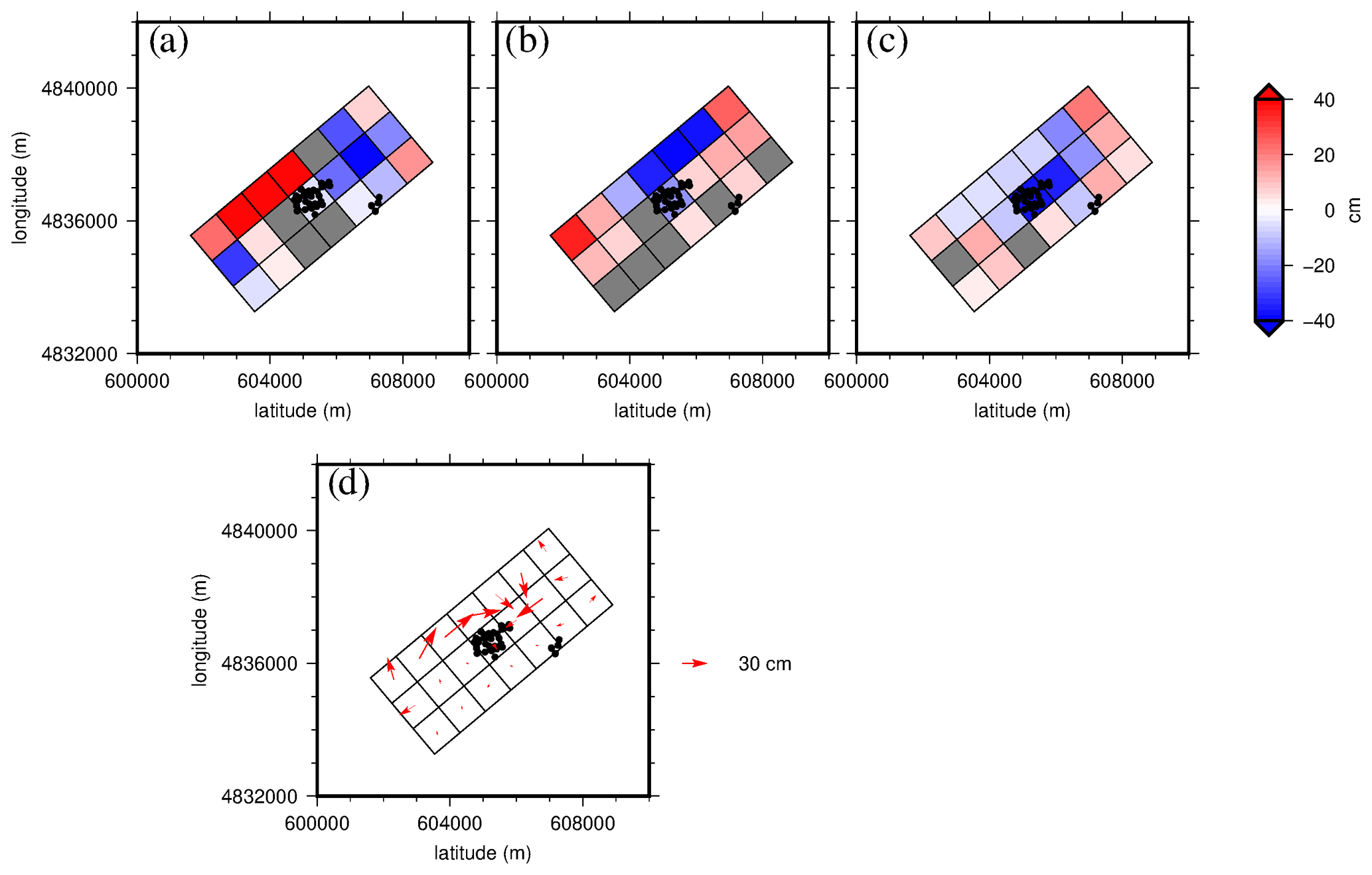
Figure 11Distribution of the significant optimal dislocation parameters: (a) strike-slip, (b) dip-slip, (c) tensile, and (d) slip displacement (strike and dip) of the hanging wall relative to the foot wall. The black dots indicate the location of well heads. Non-significant dislocations are represented in gray.
5.3.3 Residuals
In Fig. 12d to f, we represent the norm of the residual signal for each velocity component (respectively, east, north, and vertical). The mean residual values are 1.7, 3.4, and 0.7 mm yr−1 for east, north, and vertical components, but maximum residuals reach 9.6, 14.5, and 3.2 mm yr−1, respectively. For the east component (Fig. 12a), the general shape of the deformation seems to be retrieved by the inversion, while the amplitude of the velocities is underestimated by the model: high residuals (>5 mm yr−1) are localized northeast of the model and above planes 12 to 14 and 19 to 21 (Fig. 12d), and moderate residuals (between 2 to 5 mm yr−1) are observed above planes 3 and 4. The north component of the signal is the less well retrieved of all three. Large areas with high residuals are observed above and north of the exploitation (Fig. 12e). The amplitude of the signal is also underestimated by the inversion. The vertical component presents the best fit against the observed data with only small areas of moderate (above planes 1, 3 and 7) to high residuals (north of planes 18 and 19). These areas of moderate to high residuals correspond to more uncertain data for the corresponding component (Fig. 7d to f).
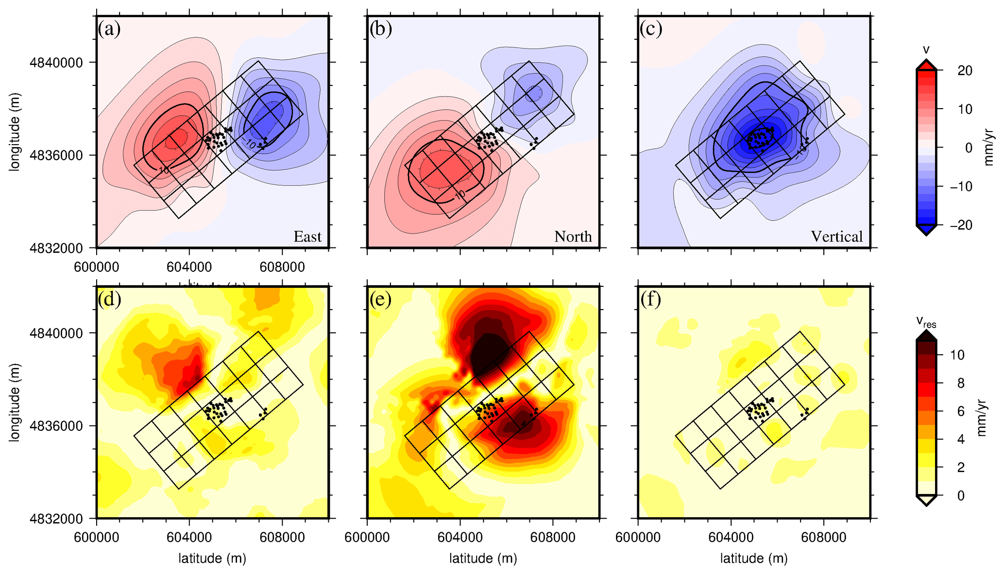
Figure 12(a) East, (b) north, and (c) vertical components of the deformation from the optimal model with the associated residuals (d, e, and f, respectively). The mean values of residual norms are estimated to 1.7, 3.4, and 0.7 mm yr−1 for the east, north, and vertical components, respectively.
In this work, the level of fit for our dataset is NRMS = 0.6 and a posteriori scatter is WRMS = 2.2 mm yr−1 (to be compared to the mean uncertainty value of 1.9 mm yr−1). Separating the east, north, and vertical velocities leads to values of WRMS of 2.3, 4.6, and 0.8 mm yr−1, respectively.
6.1 Combined velocity field
The methodology of combination requires specific conditions (see Sect. 4.1.1) among which the most restrictive are the adequacy of the periods of time considered for each technique, the radial-shaped displacement, and, depending on the exact goals of the combination (e.g., horizontal components or not), sufficient density of measurements. Hence, the time coverage of GNSS does not meet the requirements of the methodology to be included in the combination. Therefore, we use GNSS data to validate the results of the combination, given data uncertainties. Applications of the two-step process are conceivable in areas where the observed deformation is near-radial such as in gas storage, solution mining, or filling and draining of magmatic chambers.
6.2 A collection of analytical sources for the salt layer
Analytical models offer simple models to test first whether the surface deformation is only related to subsidence at depth due to the extraction of salt or whether creep occurs in the salt layers. A series of models has been computed to select the most appropriate model given the deep geometry of the reservoir and the fit to the observations. The collection of 21 planar dislocations is the best we have found considering the available datasets and their uncertainties. The inversion of the combined velocities allows us to constrain at first order the displacements of the salt layer using model 3.
The global slip displacement (Fig. 11d) indicates an overall first-order motion of the outer and deeper planes toward the center of the model where the salt exploitation is. In our case, it can be due to the fact that wells are highly connected, implying a salt flow (or short-term creep) from the entire layer towards the center of the exploitation, where there is a strong change in pressure and large cavities have opened in the salt layer. Tensile motions mainly show a closure of the central planes (from 10 to 13 and 16 to 20) with a maximum subsidence rate of 36.2 cm yr−1 at plane 11. The inversion results suggest that the deformation may not be completely radial. This demonstrates the importance of data combination, not only to better constrain the vertical component but also the three dimensions of the subsidence. To improve this 3-D field, including GNSS data in the combination would be extremely recommendable. As a result, a more detailed interpretation of the dislocations would be possible, including creep and loading (or not) of the surrounding faults.
The strong collapse observed at planes 11 and 12 is produced by the high pumping rate at extracting wells. Besides, at such depth, wells are drilled through a system of normal faults (Fig. 1). This means that openings (occurring at planes 5, 10, 13, 16, 17, 18, 19, and 20; see Fig. 11) could potentially be explained by the motions along normal faults.
Based on our model, creep occurs in the salt layers, the next step would be to produce a more global model, with an increase in the level of complexity by considering (1) the strain source with six free parameters which generate a volumetric and shear deformation (Furst et al., 2020), (2) elasto-viscoplastic laws to include salt creep, and (3) finite elements to discretize the domain.
6.3 Modeling the GNSS velocity field
In addition, the model can be validated using the available GNSS data (red arrows in Fig. 13a and b). We model the velocity at the four GNSS stations (green arrows in Fig. 13a and b) and compare it to the observations. The differences between observed and modeled data are represented in Fig. 13c and d for the horizontal and vertical velocities, respectively (note the change in arrow scale compared to Fig. 13a and b). We estimate NRMS = 16.3 and WRMS = 2.1 mm yr−1 for the horizontal velocity while NRMS = 15.9 and WRMS = 5.1 mm yr−1 for the vertical velocity. The level of correlation between the combined solution and its GNSS-only counterpart is obviously low. This may be due to the very small uncertainties associated with GNSS velocities (typical of continuous GNSS) and to the difference between the periods considered (GNSS time series cover 2 to 4 years with only 1.5 years' overlap with the InSAR coverage). In the east and north components, this may also and mostly be due to the relative location of the GNSS stations within the subsidence bowl. InSAR can hardly yield accurate horizontal velocity on specific spots unless they are optimally located (e.g., VAU3 in the east, VAU2 in the north), assuming that the period of interest is sufficient (1.5 years' overlap is short). Therefore, the global amplitude of the deformation may be preserved, but the shape may have evolved with the exploitation migrating northward. Given the high residuals between GNSS and the combined dataset, the combination would certainly improve the results. Hence, with a complete overlap of the GNSS data with InSAR and leveling data, we could use the 3-D velocity field from the GNSS data in the combination process, by readjusting InSAR over the three dimensions, independently for both ascending and descending geometries.
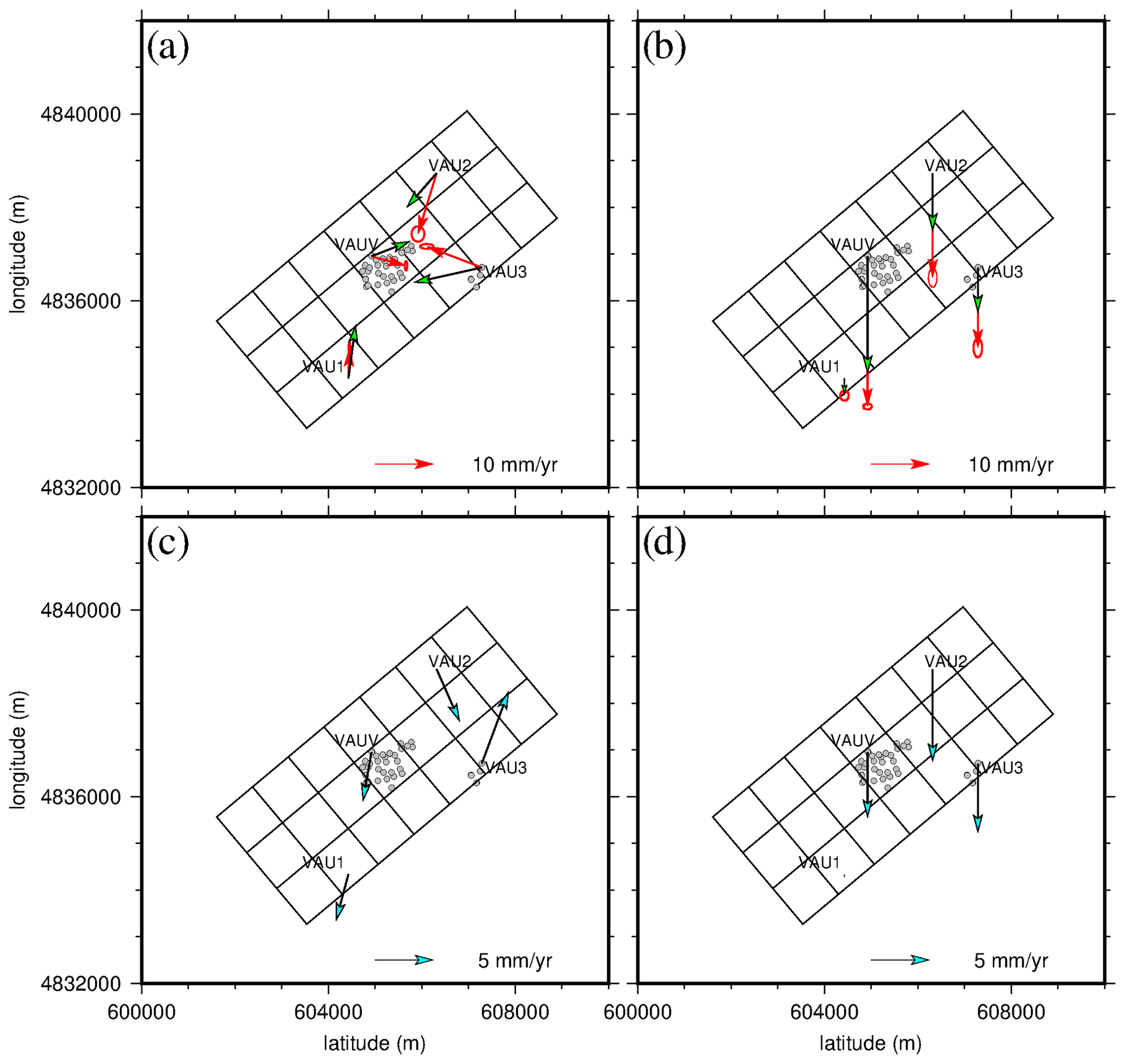
Figure 13(a) Horizontal and (b) vertical velocities at the four permanent GNSS stations. Red arrows stand for the observed data and their 2σ uncertainties and green ones for the modeled velocities using optimal parameters. Panels (c) and (d) represent the associated residuals. Note the change in arrow scale compared to (a) and (b).
6.4 Distribution of induced stress
The model constrained by the inversion of geodetic data allows us to estimate stress tensor. This modeled tensor could be compared to in situ horizontal stress orientations from the analysis of borehole breakout. They generally occur at the azimuth of the minimum horizontal stresses and perpendicular to the maximum horizontal stress. These borehole failures are generated by compressive failure of the borehole wall and result in its enlargement in the minimum horizontal stress direction. Several logs were conducted in some of Vauvert's exploitation wells and need to be analyzed. Comparing the modeled and observed stresses would permit us to assess the reliability of our model.
The microseismic activity of the exploitation was monitored between 1992 and 2007 with magnitude events ranging from −0.5 to 3 (Godano, 2009; Godano et al., 2010, 2012). Seismic activity either occurs at the decollement depth for abandoned well doublets or at depths of production zones for active well doublets. Nowadays, a new network has been deployed by the French company Magnitude (Baker Hughes) to monitor the microseismicity of the site both for the brine exploitation and for hazard management. Using the model developed in this study and the seismic events, we could also calibrate a rheological law in the area of the salt exploitation.
We developed a two-step methodology combining ascending and descending LOS with leveling data in order to overcome the difference in resolution and accuracy associated with the measurement methods. This process is specific to near-radial deformation measured by geodetic techniques whose periods of observation are consistent with each other and whose density in space and time are adequate to achieve the monitoring goals (only vertical or also horizontal). The incorporation of leveling data allowed refining the InSAR-derived deformation in height. Satellite lines of sight and flight directions must also be symmetrical enough from one acquisition geometry to the other, to extract the east component of the deformation in a first approximation. The resulting 3-D velocity field gives a spatially dense measurements of the deformation whose uncertainties are all the most reliable in those areas covered by several geodetic techniques. Due to their period of availability, slightly shifted and quite short, GNSS stations could only provide a control in a first approximation. Along with the salt layer modeling, this result demonstrated the great interest for combining timely and compliant geodetic measurements with InSAR.
We inverted this combined dataset to constrain a kinematic model of the salt layer. Because we focus on a 2-year interval for the dataset, the deformation induced by the extraction largely dominates the salt creep and an elastic model is acceptable. Hence, we proposed to assimilate the salt layer to a collection of 21 planes of dislocation with fixed positions, geometries, and orientations consistently with the salt layer characteristics. The results of the inversion indicate a collapse of the planes located beneath the exploitation and the adjacent ones at the same depth. We also identified a salt flow from the deepest and most external part of the salt layer towards the center of the exploitation due to the connections between the wells and the exploited layer. Although this model gives a first approximation of the deep deformation of the salt layer, it needs to be improved to be able to predict the deformation induced by the exploitation in the future. We suggest three levels of model improvements, involving a collection of strain sources or finite elements and elasto-viscoplastic laws for the long-term prediction.
The geodetic dataset processed and combined in the work and the optimization code are available on request from the corresponding author. The RESIF data are available from the RESIF website (DOI: https://doi.org/10.15778/resif.rg, RESIF, 2017). Maps were produced using the public domain Generic Mapping Tools (GMT) software (Wessel et al., 2013). The software can be found at https://github.com/GenericMappingTools/gmt/releases/tag/6.1.1 (GenericMappingTools, 2021).
SD developed the concept of geodetic data combination under the supervision of PV, CC, and JLC. SD performed the two-step combination of InSAR and leveling data. SLF built the inversion algorithm based on the available global optimization code. SLF designed and performed the numerical calculations for the experiments. SLF wrote the paper and designed the figures with the support of SD, PV, CC, and JLC.
The authors declare that they have no conflict of interest.
The authors want to thank the KemOne company for sharing production data and for allowing the installation of various instruments on the site and more specifically Marc Valette for sharing the geological information essential to building and interpreting the model presented in the paper. We thank the REseau NAtional GNSS Permanent, RENAG, France (RESIF, 2017), for providing two of the installed GNSS receivers. We also thank Jean Chéry, Michel Peyret, Bijan Mohammadi, and Jean-Luc Got for the inspiring discussions, their advice, and insightful comments. We thank the three anonymous reviewers for their constructive reviews of this paper.
This paper was edited by Simon McClusky and reviewed by three anonymous referees.
Abidin, H., Andreas, H., Gumilar, I., Yuwono, B., Murdohardono, D., and Supriyadi: On Integration of Geodetic Observation Results for Assessment of Land Subsidence Hazard Risk in Urban Areas of Indonesia, edited by: Rizos, C. and Willis, P., IAG 150 Years, International Association of Geodesy Symposia, vol 143, Springer, Cham., https://doi.org/10.1007/1345_2015_82, 2015. a
Astakhov, D. K., Roadarmel, W. H., Nanayakkara, A. S., and Service, H.: SPE 151017 A New Method of Characterizing the Stimulated Reservoir Volume Using Tiltmeter-Based Surface Microdeformation Measurements, in: SPE Hydraulic Fracturing Technology Conference, The Woodlands, TX, USA, 6–8 February 2012, 1–15, 2012. a
Bérest, P. and Brouard, B.: Safety of salt caverns used for underground storage blow out; mechanical instability; seepage; cavern abandonment, Oil Gas Sci. Technol., 58, 361–384, https://doi.org/10.2516/ogst:2003023, 2003. a
Bérest, P., Karimi-jafari, M., Brouard, B., Bazargan, B., Mécanique, L. D., Polytechnique, E., and Consulting, B.: In situ mechanical tests in salt caverns, Solution Mining Research Institute, Brussels, Belgium, 39 pp., 2006. a
Bérest, P., Djakeun-djizanne, H., Brouard, B., and Hévin, G.: Rapid Depresurizations: Can they lead to irreversible damage?, in: SMRI Spring Conference, Regina, Canada, 23–24 April 2012, 63–86, 2012. a
Burdack, J.: Combinaison des techniques PSinSAR et GNSS par cumul des équations normales, Master thesis, Conservatoire National des Arts et Métiers, Ecole Supérieure des Géomètres et Topographes, Le Mans, France, 68 pp., 2013. a
Camacho, A. G., González, P. J., Fernández, J., and Berrino, G.: Simultaneous inversion of surface deformation and gravity changes by means of extended bodies with a free geometry: Application to deforming calderas, J. Geophys. Res.-Solid Ea., 116, 1–15, https://doi.org/10.1029/2010JB008165, 2011. a
Catalão, J., Nico, G., Hanssen, R., and Catita, C.: Integration of Insar and Gps for Vertical Deformation Monitoring : a Case Study in Faial and Pico Islands, in: Proceedings of the Fringe 2009 Workshop, Frascati, Italy, 30 November–4 December 2009, 1–7, 2009. a
Comerci, V. and Vittori, E.: The need for a standardized methodology for quantitative assessment of natural and anthropogenic land subsidence: The Agosta (Italy) gas field case, Remote Sensing, 11, 1178, https://doi.org/10.3390/rs11101178, 2019. a
Cressie, N.: Spatial prediction and ordinary kriging, Math. Geol., 20, 405–421, https://doi.org/10.1007/BF00892986, 1988. a
Crosetto, M., Monserrat, O., Cuevas-González, M., Devanthéry, N., and Crippa, B.: Persistent Scatterer Interferometry: A review, ISPRS J. Photogramm., 115, 78–89, https://doi.org/10.1016/j.isprsjprs.2015.10.011, 2016. a
Daya, A. A. and Bejari, H.: A comparative study between simple kriging and ordinary kriging for estimating and modeling the Cu concentration in Chehlkureh deposit, SE Iran, Arab. J. Geosci., 8, 8263–8275, https://doi.org/10.1007/s12517-014-1618-1, 2015. a
Donadei, S. and Schneider, G. S.: Compressed Air Energy Storage in Underground Formations, in: Storing Energy: With Special Reference to Renewable Energy Sources, edited by: Letcher, T. M., Elsevier, 113–133, https://doi.org/10.1016/B978-0-12-803440-8.00006-3, 2016. a
Doucet, S.: Combinaison de mesures géodésiques pour l'études de la subsidence: application à la saline de Vauvert (Gard, France), PhD thesis, University of Montpellier, Montpellier, France, 234 pp., 2018. a, b
Farr, T. G. and Kobrick, M.: Shuttle radar topography mission produces a wealth of data, Eos, 81, 583–585, https://doi.org/10.1029/EO081i048p00583, 2000. a
Farr, T. G., Rosen, P. A., Caro, E., Crippen, R., Duren, R., Hensley, S., Kobrick, M., Paller, M., Rodriguez, E., Roth, L., Seal, D., Shaffer, S., Shimada, J., Umland, J., Werner, M., Oskin, M., Douglas, B., and Alsdorf, D.: The shuttle radar topography mission, Rev. Geophys., 45, 2005RG000183, https://doi.org/10.1029/2005RG000183, 2007. a
Fokker, P. A., Visser, K., Peters, E., Kunakbayeva, G., and Muntendam-Bos, A. G.: Inversion of surface subsidence data to quantify reservoir compartmentalization: A field study, J. Petrol. Sci. Eng., 96/97, 10–21, https://doi.org/10.1016/j.petrol.2012.06.032, 2012. a
Fuhrmann, T., Caro Cuenca, M., Knöpfler, A., van Leijen, F. J., Mayer, M., Westerhaus, M., Hanssen, R. F., and Heck, B.: Estimation of small surface displacements in the Upper Rhine Graben area from a combined analysis of PS-InSAR, levelling and GNSS data, Geophys. J. Int., 203, 614–631, https://doi.org/10.1093/gji/ggv328, 2015. a, b
Furst, S., Chéry, J., Peyret, M., and Mohammadi, B.: Tiltmeter data inversion to characterize a strain tensor source at depth: application to reservoir monitoring, J. Geodesy., 94, 48, https://doi.org/10.1007/s00190-020-01377-5, 2020. a
Galgana, G. A., Newman, A. V., Hamburger, M. W., and Solidum, R. U.: Geodetic observations and modeling of time-varying deformation at Taal Volcano, Philippines, J. Volcanol. Geoth. Res., 271, 11–23, https://doi.org/10.1016/j.jvolgeores.2013.11.005, 2014. a
GenericMappingTools: gmt, available at: https://github.com/GenericMappingTools/gmt/releases/tag/6.1.1, last access: 7 January 2021. a
Gillhaus, A. and Horvath, P. L.: Compilation of geological and geotechnical data of worldwide domal salt deposits and domal salt cavern fields, Solution Mining Research Insitute and KBB Underground Technologies GmbH, Clarks Summit, PA, USA, 2008. a
Godano, M.: Etude théorique sur le calcul des mécanismes au foyer dans un réservoir et application à la sismicité de la saline de Vauvert (Gard), PhD thesis, Université Nice Sophia Antipolis, Nice, France, 330 pp., 2009. a
Godano, M., Gaucher, E., Bardainne, T., Regnier, M., Deschamps, A., and Valette, M.: Assessment of focal mechanisms of microseismic events computed from two three-component receivers: Application to the Arkema-Vauvert field (France), Geophys. Prospect., 58, 775–790, https://doi.org/10.1111/j.1365-2478.2010.00906.x, 2010. a
Godano, M., Bardainne, T., Regnier, M., Deschamps, A., and Valette, M.: Spatial and temporal evolution of a microseismic swarm induced by water injection in the Arkema-Vauvert salt field (southern France), Geophys. J. Int., 188, 274–292, https://doi.org/10.1111/j.1365-246X.2011.05257.x, 2012. a
Hager, B. H., King, R. W., and Murray, M. H.: Measurement of Crustal Deformation Using the Global Positioning System, Annu. Rev. Earth Pl. Sc., 19, 351–382, https://doi.org/10.1146/annurev.ea.19.050191.002031, 1991. a
Hammond, W., Lib, Z., and Plaga, H.: Integrated Insar and Gps Studies of Crustal Deformation in the Western Great Basin, Western United States, Int. Arch. Photogramm., XXXVIII, 39–43, 2010. a
Hastaoglu, K. O., Poyraz, F., Turk, T., Yılmaz, I., Kocbulut, F., Demirel, M., Sanli, U., Duman, H., and Balik Sanli, F.: Investigation of the success of monitoring slow motion landslides using Persistent Scatterer Interferometry and GNSS methods, Surv. Rev., 50, 475–486, https://doi.org/10.1080/00396265.2017.1295631, 2017. a
Hengl, T., Heuvelink, G. B., and Stein, A.: A generic framework for spatial prediction of soil variables based on regression-kriging, Geoderma, 120, 75–93, https://doi.org/10.1016/j.geoderma.2003.08.018, 2004. a, b
Hengl, T., Heuvelink, G. B., and Rossiter, D. G.: About regression-kriging: From equations to case studies, Comput. Geosci., 120, 75–93, https://doi.org/10.1016/j.cageo.2007.05.001, 2007. a
Herring, T. A., King, R. W., Floyd, M. A., and McClusky, S. C.: Introduction to GAMIT/GLOBK, Release 10.6, Tech. rep., Massachusetts Institute of Technology, Cambridge, USA, 48 pp., 2015. a
Hooper, A., Zebker, H., Segall, P., and Kampes, B.: A new method for measuring deformation on volcanoes and other natural terrains using InSAR persistent scatterers, Geophys. Res. Lett., 31, 1–5, https://doi.org/10.1029/2004GL021737, 2004. a
Ivorra, B. and Mohammadi, B.: Semi-deterministic global optimization method, J. Optimiz. Theory App., 135, 549–561, https://doi.org/10.1007/s10957-007-9251-8, 2007. a
Karila, K., Karjalainen, M., Hyyppä, J., Koskinen, J., Saaranen, V., and Rouhiainen, P.: A comparison of precise leveling and Persistent Scatterer SAR Interferometry for building subsidence rate measurement, ISPRS Int. Geo-Inf., 2, 797–816, https://doi.org/10.3390/ijgi2030797, 2013. a
Ligas, M. and Kulczycki, M.: Kriging approach for local height transformations, Geodesy and Cartography, 63, 25–37, https://doi.org/10.2478/geocart-2014-0002, 2015. a
Lu, C. H., Ni, C. F., Chang, C. P., Yen, J. Y., and Hung, W. C.: Combination with precise leveling and PSInSAR observations to quantify pumping-induced land subsidence in central Taiwan, Proc. IAHS, 372, 77–82, https://doi.org/10.5194/piahs-372-77-2015, 2015. a, b
Lundgren, P., Hetland, E. A., Liu, Z., and Fielding, E. J.: Southern San Andreas-San Jacinto fault system slip rates estimated from earthquake cycle models constrained by GPS and interferometric synthetic aperture radar observations, J. Geophys. Res.-Sol. Ea., 114, 1–18, https://doi.org/10.1029/2008JB005996, 2009. a
Maisons, C., Raucoules, D., and Carnec, C.: Monitoring of slow ground deformation by satellite differential radar-interferometry. A reference case study, Solution Mining Research Institute, Brussels, Belgium, 10 pp., 2006. a
McCaffrey, R.: Block kinematics of the Pacific-North America plate boundary in the southwestern United States from inversion of GPS, seismological, and geologic data, J. Geophys. Res.-Sol. Ea., 110, 1–27, https://doi.org/10.1029/2004JB003307, 2005. a, b
Mogi, K.: Relations between the eruptions of various volcanoes and the deformations of the ground surfaces around them, 36, 99–134, https://doi.org/10.1016/j.epsl.2004.04.016, 1958. a, b
Mohammadi, B.: Backward uncertainty propagation in shape optimization, Int. J. Numer. Meth. Fl., 80, 285–305, https://doi.org/10.1002/fld.4077, 2016. a
Mohammadi, B. and Pironneau, O.: Applied Shape Optimization for fluids, Oxford University Press, Oxford, UK, 2009. a
Okada, Y.: Internal deformation due to shear and tensile faults in a half-space, B. Seismol. Soc. Am., 82, 1018–1040, 1992. a, b, c, d
Pebesma, E. J.: The role of external variables and GIS databases in geostatistical analysis, T. GIS, 10, 615–632, https://doi.org/10.1111/j.1467-9671.2006.01015.x, 2006. a
Peltier, A., Staudacher, T., and Bachèlery, P.: Constraints on magma transfers and structures involved in the 2003 activity at Piton de La Fournaise from displacement data, J. Geophys. Res.-Sol. Ea., 112, 1–16, https://doi.org/10.1029/2006JB004379, 2007. a
Peltier, A., Froger, J., Villeneuve, N., and Catry, T.: Assessing the reliability and consistency of InSAR and GNSS data for retrieving 3D-displacement rapid changes, the example of the 2015 Piton de la Fournaise eruptions, J. Volcanol. Geoth. Res., 344, 106–120, https://doi.org/10.1016/j.jvolgeores.2017.03.027, 2017. a, b
Raucoules, D., Maisons, C., Carnec, C., Le Mouelic, S., King, C., and Hosford, S.: Monitoring of slow ground deformation by ERS radar interferometry on the Vauvert salt mine (France): Comparison with ground-based measurement, Remote Sens. Environ., 88, 468–478, https://doi.org/10.1016/j.rse.2003.09.005, 2003. a, b, c, d, e, f, g, h, i
Raucoules, D., Maisons, C., and Carnec, C.: Monitoring subsidence on the Vauvert salt mine using radar interferometry, in: Journées Nationales de Géotechnique et de Géologie de l'ingénieur, Lille, France, 28–30 June 2004, 413–417, 2004. a
Reilinger, R., McClusky, S., Vernant, P., Lawrence, S., Ergintav, S., Cakmak, R., Ozener, H., Kadirov, F., Guliev, I., Stepanyan, R., Nadariya, M., Hahubia, G., Mahmoud, S., Sakr, K., ArRajehi, A., Paradissis, D., Al-Aydrus, A., Prilepin, M., Guseva, T., Evren, E., Dmitrotsa, A., Filikov, S. V., Gomez, F., Al-Ghazzi, R., and Karam, G.: GPS constraints on continental deformation in the Africa-Arabia-Eurasia continental collision zone and implications for the dynamics of plate interactions, J. Geophys. Res.-Sol. Ea., 111, 1–26, https://doi.org/10.1029/2005JB004051, 2006. a
RESIF: RESIF-RENAG French national Geodetic Network, RESIF – Réseau Sismologique et géodésique Français, https://doi.org/10.15778/resif.rg, 2017., a, b
Séranne, M., Benedicto, A., Labaum, P., Truffert, C., and Pascal, G.: Structural style and evolution of the Gulf of Lion Oligo-Miocene rifting: role of the Pyrenean orogeny, Mar. Petrol. Geol., 12, 809–820, https://doi.org/10.1016/0264-8172(95)98849-Z, 1995. a
Valette, M.: Etude structurale du gisement salifère oligocène de Vauvert (Gard), PhD thesis, Université de Montpellier, Montpellier, France, 229 pp., 1991. a
Valette, M. and Benedicto, A.: Gravity thrust halotectonics in the extensional Camargue basin (Gulf of Lion margin, SE France), B. Soc. Géol. Fr., 166, 137–147, 1995. a, b, c, d, e
Van Sambeek, L. L.: Evaluating Cavern Tests and Surface Subsidence Using Simple Numerical Models, Seventh Symposium on salt, Kyoto, Japan, 6–9 April 1992, 433–439, ISBN 0444891439, 1993. a, b, c
Vasco, D. W., Ferretti, A., and Novali, F.: Reservoir monitoring and characterization using satellite geodetic data: Interferometric synthetic aperture radar observations from the Krechba field, Algeria, Geophysics, 73, WA113, https://doi.org/10.1190/1.2981184, 2008. a
Wessel, P., Smith, W. H., Scharroo, R., Luis, J., and Wobbe, F.: Generic mapping tools: Improved version released, Eos, 94, 409–410, https://doi.org/10.1002/2013EO450001, 2013. a
Wright, T. J., Parsons, B. E., and Lu, Z.: Toward mapping surface deformation in three dimensions using InSAR, Geophys. Res. Lett., 31, 1–5, https://doi.org/10.1029/2003GL018827, 2004. a
Yamamoto, J. K.: Comparing ordinary kriging interpolation variance and indicator kriging conditional variance for assessing uncertainties at unsampled locations, in: Proceedings of the 32nd Int. Symposium on the Application of Computers and Operations Research in the Mineral Industry, APCOM 2005, Tucson, USA, 30 March–1 April 2005, 265–272, https://doi.org/10.1201/9781439833407.ch34, 2005. a