Changepoint detection in seismic double-difference data: application of a trans-dimensional algorithm to data-space exploration

Double-difference (DD) seismic data are widely used to define elasticity distribution in the Earth's interior and its variation in time. DD data are often pre-processed from earthquake recordings through expert opinion, whereby pairs of earthquakes are selected based on some user-defined criteria and DD data are computed from the selected pairs. We develop a novel methodology for preparing DD seismic data based on a trans-dimensional algorithm, without imposing pre-defined criteria on the selection of event pairs. We apply it to a seismic database recorded on the flank of Katla volcano (Iceland), where elasticity variations in time have been indicated. Our approach quantitatively defines the presence of changepoints that separate the seismic events in time windows. Within each time window, the DD data are consistent with the hypothesis of time-invariant elasticity in the subsurface, and DD data can be safely used in subsequent analysis. Due to the parsimonious behaviour of the trans-dimensional algorithm, only changepoints supported by the data are retrieved. Our results indicate the following: (a) retrieved changepoints are consistent with first-order variations in the data (i.e. most striking changes in the amplitude of DD data are correctly reproduced in the changepoint distribution in time); (b) changepoint locations in time correlate neither with changes in seismicity rate nor with changes in waveform similarity (measured through the cross-correlation coefficients); and (c) the changepoint distribution in time seems to be insensitive to variations in the seismic network geometry during the experiment. Our results demonstrate that trans-dimensional algorithms can be effectively applied to pre-processing of geophysical data before the application of standard routines (e.g. before using them to solve standard geophysical inverse problems).

1 Introduction

Data preparation is a daily routine in the working life of geoscientists. Before using data to get insights into the Earth system, geoscientists try to deeply understand their data sets to avoid introducing, e.g. instrumental issues, redundant data, unwanted structures such as data density anomalies, and many others (Yin and Pillet, 2006; Berardino et al., 2002; Lohman and Simons, 2005). All the activities for preliminary data analysis can be considered an exploration of the “data space” (Tarantola, 2005) and are mainly based on expert opinion. Previous experience drives scientists in selecting the most trustable portion of their experiments by cleaning data sets before using them for getting new knowledge about Earth model parameters. There are two main reasons for moving a step forward from expert opinion. First, the huge amount of (often multidisciplinary) data accumulated in geosciences in the last decade requires more and more data screening and preparation, sometimes involving multidisciplinary expertise. Research activities could greatly benefit from a more automated exploration of the data space able to ease preparatory tasks. Second, expert opinion is a human activity and is mainly based on dual categories, e.g. good or bad data, and cannot easily handle a continuous probability distribution over the data (i.e. expert opinion cannot easily associate a continuous “confidence” measure with each data point).

In recent years, in the framework of Bayesian inference, exploration of the data space has been introduced in a few cases to “explore” unknown features of the data sets. For example, the so-called hierarchical Bayes' approach has been introduced to estimate data uncertainties from the data themselves (Malinverno and Briggs, 2004). More complex hierarchical Bayes' approaches have been developed to measure the data correlation as well (e.g. Bodin et al., 2012a; Galetti et al., 2016) or to evaluate an error model (e.g. Dettmer and Dosso, 2012). The exploration of the data space in all these studies implies considering some additional unknowns (e.g. data uncertainties or error correlation length), so-called hyper-parameters or nuisance parameters, and estimating them directly from the data. A step forward in the exploration of the data space has been presented by Steininger et al. (2013) and Xiang et al. (2018), who used a data-space exploration approach to evaluate the performance of two different error models directly from the data. In such studies, the number of hyper-parameters considered is not fixed but can assume two different values (1 or 2) depending on the error model considered. Another interesting, recent case of exploration of the data space is represented by the work of Tilmann et al. (2020), in which the authors used Bayesian inference to separate the data into two sets: “outliers” and “regular”. In this case, the data themselves are probabilistically evaluated to understand their contribution to the final solution as regular data or outlier data; i.e. the data are classified into two different families according to their coherence with the hypothesis of being regular data or not.

In this study, we push the exploration of data space in a new direction. We develop an algorithm for computing Bayesian inference specifically for the exploration of the data space. Exploration of the data space is performed through a trans-dimensional algorithm (e.g. Malinverno, 2002; Sambridge et al., 2006) so that the number of hyper-parameters is neither fixed nor limited to 1 or 2. We represent data structure as partitions of the covariance matrix of uncertainties, i.e. changepoints that create sub-matrices of the covariance matrix with homogeneous characteristics, with the number of partitions not dictated by the user but derived by the data themselves in a Bayesian sense (i.e. we obtain a posterior probability distribution, PPD, of the number of partitions). In this way, similar to Tilmann et al. (2020), portions of data can be classified and used differently in the subsequent steps of the analysis.

We apply our algorithm to prepare a widely exploited type of seismic data set, the seismic double-difference (DD) data set, that has been used as input in seismic tomography for defining subsurface elasticity (e.g. Zhang and Thurber, 2003) and its variation in time (e.g. so-called “time-lapse tomography”; Caló et al., 2011; Zhang and Zhang, 2015). DD data need to be reconstructed from specific partitions of the original data (i.e. seismic events). Subjective choices have a great impact on the definition of DD data. In particular, such choices can be used to limit the number of DD data themselves, and the selection, in turn, could introduce biases in the subsequent definition of the elastic model and its variations in time. We apply our algorithm to statistically define, in a more objective way, the distribution of partitions in the DD data. We show how a more data-driven approach can obviate expert-driven data selection and can be used as a preliminary tool for e.g. time-lapse seismic tomography.

1.1 Double-difference data in seismology

Double-difference seismic data are widely used for relocating seismic events and imaging the subsurface (e.g. Waldhauser and Ellsworth, 2000; Roecker et al., 2021). DD data rely on the assumption of (nearly) co-located events for which seismic recordings have been obtained from the same station (Zhang and Thurber, 2003) or for the same pair of stations (e.g. Guo and Zhang, 2016). The concept of co-located events relies on expert opinion. It is generally assumed a priori as a maximum distance between hypocentres in order to consider a pair of events to be included in the DD data, together with a high value of cross-correlation for their waveforms. A DD datum is the differential travel time for the selected pair of events. The same scheme has been applied to more complex analyses, such as full waveform inversion (Lin and Huang, 2015). Based on the assumption of nearly co-located events, the information contained in the DD datum can be used to refine event locations (e.g. small events referred to a master event; Waldhauser and Ellsworth, 2000) or the seismic properties of the rocks in the area where events are clustered (e.g. Zhang and Thurber, 2003). In recent years, seismic monitoring of subsurface processes has also been realized through seismic tomography (e.g. Chiarabba et al., 2020), in particular with the analysis of DD data: rock weakening due to mining activities (Qian et al., 2018; Ma et al., 2020; Luxbacher et al., 2008), granite fracturing during geothermal well stimulation (Caló et al., 2011; Caló and Dorbath, 2013), and oil and gas operations (Zhang et al., 2006). For monitoring purposes, an additional assumption is considered during DD data preparation: elastic properties of the media traversed by the seismic waves should not change between the occurrence of the selected event pairs. This fact implies the computation of the so-called time-lapse analysis, wherein pre-defined time windows are considered and static images of the subsurface (Caló et al., 2011), or differential elastic models (Qian et al., 2018), are reconstructed for each time window. In any case, the most relevant issue in time-lapse tomography remains how to define the time windows, which artificially separate events and prevent their coupling to obtain DD data. How many time windows are meaningful to construct DD data? And what should be their time lengths? This issue is critical due to the dependence of the number of DD data on the number of paired events and thus from the number of time windows, as schematically shown in Fig. 1.

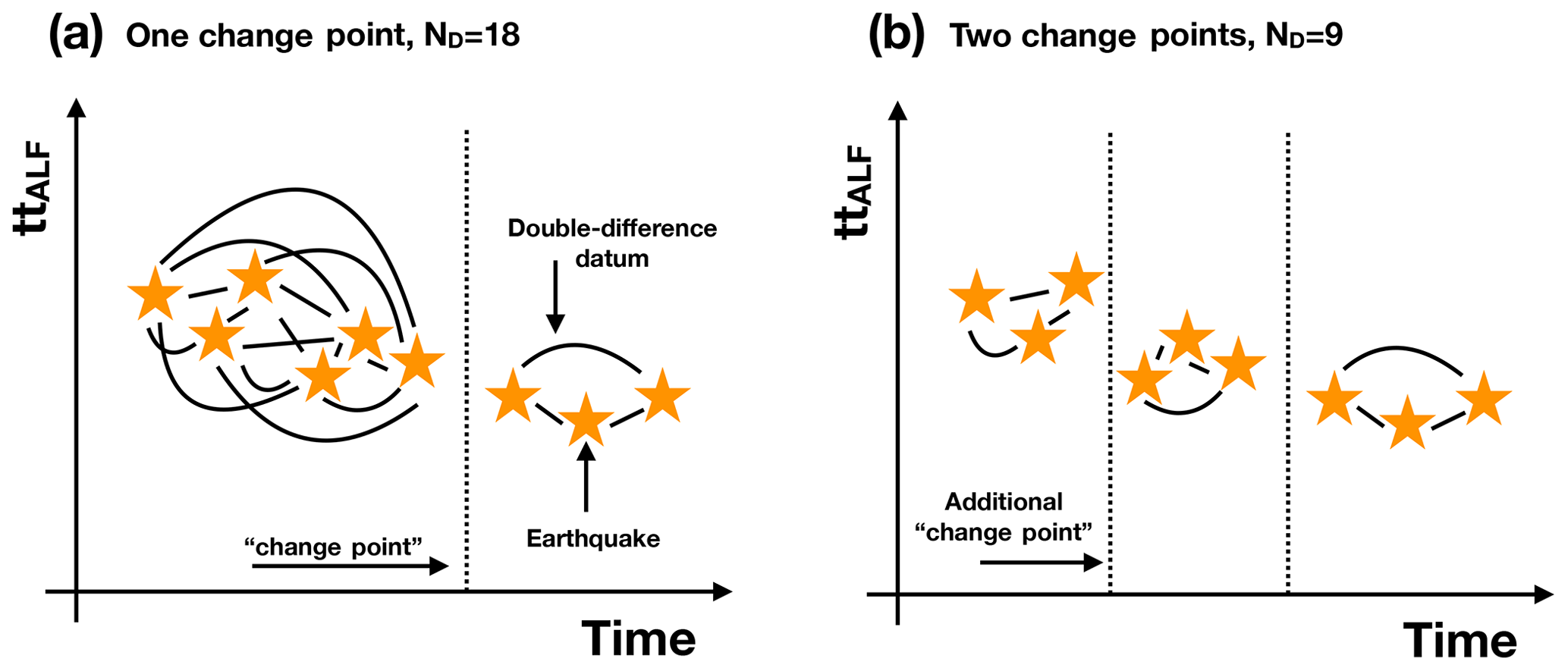
Figure 1 Schematic example of the standard preparation of DD data in different time windows. Time windows are defined by changepoints (also called “hard partitions”). Here, for the sake of simplicity, we represent the travel time to station ALF for each seismic event (yellow stars) as a function of origin time. A DD datum (curved black line) is prepared for each pair of events not separated by a changepoint. (a) Here, only one changepoint is present, so N_D=18 DD data can be prepared. (b) In the case of two changepoints, only N_D=9 DD data can be prepared.

The definition of the set of time windows, on which the sequence of 3D time-lapse tomographic inversions should be computed, demands expert opinion. There are three main possibilities in time-lapse tomography: (a) imposing time windows based on known seismic history (before and after a known, relevant seismic event: Young and Maxwell, 1992; Chiarabba et al., 2020), (b) keeping the same length for all time windows (e.g. 1 d; Qian et al., 2018), or (c) trying to have the same amount of data in all the time windows (e.g. Patanè et al., 2006; Kerr, 2011; Zhang and Zhang, 2015). In other cases, the lengths of the time windows vary based on research needs (e.g. Caló et al., 2011). A human-defined set of time windows might mask the real variations of the physical properties, in which case the time evolution of the elastic model found could be not associated with the investigated geophysical process.

Here, we tackle the issue of defining the number and time length of the time windows in DD data preparation through a novel approach. To simplify the experiment, we focus on closely associated events recorded on a volcanic edifice in Iceland. Such a cluster of events, which spans no more than 100 m in diameter, is considered a source of repeating events that are recorded from a seismic station 6 km away for more than 2 years continuously. In this way, we assume perfectly co-located events and we can focus on time variations of DD data. More generally, the novel approach can be applied to both temporal and spatial associations (i.e. to define both time windows and spatial length for pairing events and composing DD data).

1.2 Background on Bayesian inference, Markov chain Monte Carlo sampling, and trans-dimensional algorithms

Geophysical inverse problems have been solved for a long time following direct search or linearized inversion schemes due to the limited number of computations needed to obtain a solution. Such solutions have been given in the form of a single “final” model presented as representative of the Earth's physical properties. Thanks to the computational resources now available, such approaches are outdated for more sophisticated and CPU-time-consuming workflows, in which multiple models are evaluated and compared, to obtain a wider view of the Earth's physical properties. Algorithms based on Bayesian inference belong to this second category, for which the “solution” is no longer a single model but a distribution of probability on the possible value of the investigated parameters, following Bayes' theorem (Bayes, 1763):

$$\begin{array}{}\text{(1)}& {\displaystyle }{\displaystyle }p(\mathit{m}\mid \mathit{d})={\displaystyle \frac{p\left(\mathit{m}\right)p(\mathit{d}\mid \mathit{m})}{p\left(\mathit{d}\right)}},\end{array}$$

where p(m∣d) represents the information obtained from the model parameters m through the data d, the so-called posterior probability distribution (PPD) or simply “posterior”. Such information is obtained combining the prior knowledge of the model: p(m), with the likelihood of the model given the data, p(d∣m). The denominator of the right term is called “evidence” and represents the probability of the data in the model space:

$$\begin{array}{}\text{(2)}& {\displaystyle }{\displaystyle }p\left(\mathit{d}\right)=\int p\left(\mathit{m}\right)p(\mathit{d}\mid \mathit{m})\mathrm{d}\mathit{m}.\end{array}$$

The evidence is a high-dimensional integral that normalizes the PPD. It is generally difficult to compute, and thus methods that do not require its computation (such as Markov chain Monte Carlo, McMC; see below) are widely used in Bayesian inference.

The likelihood of the data for a given model is necessary to evaluate and compare different sets of model parameters. It is generally expressed as

$$\begin{array}{}\text{(3)}& {\displaystyle }{\displaystyle }L\left(\mathit{m}\right)=p(\mathit{d}\mid \mathit{m})={\displaystyle \frac{\mathrm{1}}{\left(\mathrm{2}\mathit{\pi }\right|{\mathbf{C}}_{\mathit{e}}|{)}^{\mathrm{1}/\mathrm{2}}}}{e}^{-\frac{\mathrm{1}}{\mathrm{2}}\mathit{\varphi }},\end{array}$$

where ϕ represents the fit between model prediction p_i and the actual value of the ith observation o_i, i.e. the residuals ${\mathit{e}}_i=(o_i-p_i)$, through the covariance matrix of the uncertainties C_e:

$$\begin{array}{}\text{(4)}& {\displaystyle }{\displaystyle }\mathit{\varphi }={\mathit{e}}^{\mathrm{T}}{\mathbf{C}}_{\mathit{e}}^{-\mathrm{1}}\mathit{e}.\end{array}$$

Due to the difficulties in computing the evidence and the analytic solution of Eq. (1), and thanks to the improved computational resources, in the last 2 decades the emerging trend in Bayesian inference has been represented by “sampling methods”, in which the direct computation of Eq. (1) is replaced by the sampling of the model space according to the PPD (Sambridge and Mosegaard, 2002). One of the most famous sampling methods is called Markov chain Monte Carlo, for which the chain samples the model space according to probability rules, such as the Gibbs sampler or Metropolis rule (Metropolis et al., 1953; Gelman et al., 1996). Briefly, starting from a given point in the model space called the current model, a new point of the model space called the candidate model is proposed and evaluated according to some rules based on the PPD. In particular, the Metropolis rule coupled to the approach developed in Mosegaard and Tarantola (1995), which is the workflow adopted in this study, accepts or rejects moving from a current model to a candidate model according to the ratio of their likelihoods, i.e.

$$\begin{array}{}\text{(5)}& {\displaystyle }{\displaystyle }\mathit{\alpha }=L\left({\mathit{m}}_{\text{cand}}\right)/L\left({\mathit{m}}_{\text{cur}}\right).\end{array}$$

This is a simplified version of a more general formulation of the acceptance probability in Metropolis-based McMC (Gallagher et al., 2009). It is worth noting that our workflow does not directly specify the dimensionality of the model space. In fact, following the recent advancements in the solution of geophysical inverse problems, we do not consider models with a fixed number of parameters, but we make use of the so-called trans-dimensional (trans-D) algorithm and propose candidate models with a different number of dimensions with respect to the current models. This approach is called trans-D sampling, and it has been widely used for the solution of geophysical inverse problems in the last decades (Malinverno, 2002; Sambridge et al., 2006; Bodin et al., 2012a; Dettmer et al., 2014; Mandolesi et al., 2018; Poggiali et al., 2019). Trans-D algorithms have been proven to be intrinsically “parsimonious” (Malinverno, 2002), and thus they preferably sample simpler models with respect to complex ones. This is one of the most important characteristics of trans-D algorithms, enabling a fully data-driven solution for the model parameters.

The covariance matrix C_e plays an important role in Eq. (5). In fact, it (inversely) scales the differences between the observations and the predictions (vector e) in Eq. (4). Having larger values in the entries of C_e means that differences between observations and predictions are less relevant and more candidate models can be accepted during the McMC sampling through the Metropolis rule. Conversely, larger values in C_e decrease the overall1 likelihood due to an increase in the denominator in Eq. (3). If the entries in C_e related to a certain observation are all larger with respect to the entries related to other observations, such observations will have limited importance in the McMC sampling. Defining an appropriate C_e becomes fundamental for correctly driving the McMC sampling of the PPD.

2 An algorithm for exploration of double-difference data space

What happens to the DD data set if we create a hard partition in time, i.e. if we artificially separate some events from the others? As clearly illustrated in Fig. 1, the number of data N_D in the DD data set varies, decreasing for an increasing number of hard partitions. From a Bayesian point of view, this is not admissible because Eqs. (3) and (5) need to consider the same number of data points in two models to allow their comparison (see also Tilmann et al., 2020).

Our novel approach to solve this issue relies on the introduction of a family of “hyper-parameters”, which represent the partitions of the events, and such hyper-parameters are used for scaling the different entries in the covariance matrix C_e. In our approach, the number of hyper-parameters in the family is not fixed, but it is directly derived from the data themselves. Hyper-parameters have been introduced in geophysical inversions for estimating the data uncertainties, expressed, for example, as the variance of a Gaussian distribution (Malinverno and Briggs, 2004). Hyper-parameters are generally part of the model vector together with physical parameters. As stated in Bodin et al. (2012b), estimated hyper-parameters not only account for measurement uncertainties, but also include other contributions that build up the uncertainty in the geophysical inversions, such as simplification of the physics included in the forward solutions or simplified model parameterization. Hyper-parameters have been used to estimate uncertainty models (Dettmer and Dosso, 2012; Galetti et al., 2016) or to discriminate between two different families of uncertainty models (Steininger et al., 2013; Xiang et al., 2018). In this last case, the number of hyper-parameters belonging to a model vector is not constant but can be one or two depending on the family. More recently, a nuisance parameter has been introduced to evaluate the probability of each datum to belong to the regular data or to the outliers (Tilmann et al., 2020).

For the DD case, we introduce a family of hyper-parameters to estimate which portions of the DD data violate our initial assumptions. In fact, in our assumptions, double-difference data are computed from pairs of seismic events that occurred in the same rock volume, recorded at the same seismic station. For perfectly co-located events, and in the absence of any change in the rock seismic velocity field between the first and the second event, double-difference measurements should have a mean of 0 and should be distributed following a simple Gaussian error model, which can be a represented by the (diagonal) covariance matrix ${\mathbf{C}}_{\mathit{e}}^{\ast }$, with the DD uncertainties along the diagonal. Here we assume no correlation between uncertainties computed for two different event pairs (see Appendix B1 for the definition of ${\mathbf{C}}_{\mathit{e}}^{\ast }$ from our data). In this case, the value of the fit $\stackrel{\mathrm{̃}}{\mathit{\varphi }}$ expressed as

$$\begin{array}{}\text{(6)}& {\displaystyle }{\displaystyle }\stackrel{\mathrm{̃}}{\mathit{\varphi }}={\mathit{d}}^{\mathrm{T}}{{\mathbf{C}}_{\mathit{e}}^{\ast }}^{-\mathrm{1}}\mathit{d},\end{array}$$

with d the DD data vector, should be close to N_D (N_D is the number of DD data, i.e. the length of the DD data vector).

When the value of $\stackrel{\mathrm{̃}}{\mathit{\varphi }}$ significantly deviates from N_D, a modified covariance matrix C_e(m) should be adopted, whereby the portion of the data inconsistent with the hypotheses are considered differently from the portions of DD data that do not violate the hypotheses. The new modified covariance matrix C_e(m) is obtained as

$$\begin{array}{}\text{(7)}& {\displaystyle }{\displaystyle }{\mathbf{C}}_{\mathit{e}}\left(\mathit{m}\right)={\mathbf{W}}^{-\mathrm{1}}\left(\mathit{m}\right){\mathbf{C}}_{\mathit{e}}^{\ast }{\mathbf{W}}^{-\mathrm{1}}\left(\mathit{m}\right),\end{array}$$

where the matrix W(m) is a diagonal matrix that depends on the weight for each DD datum based on the hyper-parameters. It is noteworthy that if we use Eq. (7) in Eq. (3), we see that in our case the dependence of the likelihood function on the model no longer resides in the residuals, as is generally the case in geophysical inverse problems, but only in the covariance matrix. However, for a simple case such as ours, we highlight the fact that this dependence could in principle be moved back to the residuals if we allow the physical assumptions to be variable in time (i.e. if we allow the elastic model to change in time, which in our assumption cannot).

Following a Bayesian inference approach, we reconstruct the statistical distribution of the hyper-parameters (i.e. event partitions) in time through trans-dimensional McMC sampling. The fully novel idea in our algorithm resides in the trans-dimensional behaviour of our exploration of the data space. In fact, the number of hyper-parameters in the model (and thus the number of partitions of ${\mathbf{C}}_{\mathit{e}}^{\ast }$) is not fixed and can change along the McMC sampling. At the end of the McMC sampling, we can compute a PPD of the number of partitions in the problem, which is information fully prescribed from the data and priors. In Fig. 2, we present a flowchart of our algorithm indicating the main elements. The algorithm follows a standard McMC sampling scheme based on the Metropolis rule. First of all, we need to define the model parameterization, i.e. how we formalize our family of hyper-parameters (Sect. 2.1). Thus, an explicit definition of the prior probability distribution on the parameters which compose the models is needed (Sect. 2.2). Such parameters are perturbed along the McMC sampling following prescribed rules which are randomly applied to propose a new candidate model (Sect. 2.3). Finally, we present the DD data, which will be used to test our algorithm, and how we obtain them (Sect. 2.4 and Appendix B).

Figure 2 Flowchart of the algorithm. The grey-shaded box indicates the element which can be shared on multiple CPUs on a cluster.

2.1 Model parameterization

In our algorithm, a model is described by a set of k changepoints that define the partitions of ${\mathbf{C}}_{\mathit{e}}^{\ast }$ and their associated quantities: that is, $\mathit{m}=(k,{\mathit{T}}_k,{\mathit{\pi }}_k)$. The k vector T_k represents the time occurrence of the k changepoints, whereas the k vector π_k contains the weights associated with each changepoint. We assume that a DD datum d_ij, associated with events i and j, retains its original variance ${\mathit{\sigma }}_{ij}^{\mathrm{2}}$ if no changepoint occurs between OT_i and OT_j. Otherwise, its importance is modified with weight W_ij(m):

$$\begin{array}{}\text{(8)}& {\displaystyle }{\displaystyle }{\mathbf{W}}_{ij}\left(\mathit{m}\right)={\mathrm{10}}^{-w_{ij}\left(\mathit{m}\right)},\end{array}$$

where w_ij is computed as

$$\begin{array}{}\text{(9)}& {\displaystyle }{\displaystyle }{w}_{ij}\left(\mathit{m}\right)=\sum _{p=\mathrm{1}}^k{\mathit{\pi }}_p\text{if}{\text{OT}}_i<T_p<{\text{OT}}_j,\end{array}$$

recalling that W is a N_D×N_D diagonal matrix and W_ij represents the element along the diagonal associated with DD datum d_ij. Following our approach for defining the w_ij(m), specifically the sum of the values associated with the relevant changepoints, we assume that a pair of “distant” events in time has more probability of being “separated” by one or more changepoints and thus of having a lower weight W_ij(m). This assumption reflects the standard process of DD data, in which distant (in space and/or time) events are almost never paired in DD data sets. However, if no changepoints are present between distant events, our trans-dimensional approach still works, reducing the number of changepoints to the minimum. Several synthetic tests, shown in Appendix A, demonstrate that non-necessary changepoints are removed from the family due to the parsimoniousness of the trans-dimensional algorithm, and new ones have limited probability of being accepted in the family.

2.2 Prior information

Uniform prior probability distributions are selected for our inverse problem. Here, the number of changepoints is bounded between 0 and 100. Changepoints can be distributed everywhere in time between 2011.5 and 2013.7. To make the algorithm more efficient, we set a minimum distance between two changepoints as large as 0.5 d (Malinverno, 2002). Changepoint weights π_k follow a uniform prior probability distribution between 0.0 and 1.0.

2.3 Candidate selection

Having an efficient workflow for carrying out the McMC sampling is fundamental for keeping the CPU time within acceptable limits. From a theoretical point of view, any recipe can be implemented at the core of the McMC due to the fact that results (i.e. Eq. 1) do not depend on the McMC details¹; i.e. the same prior information and the same data will give the same PPD, whatever recipe is selected for the McMC sampling. However, inefficient recipes can take too long to adequately sample the PPD, and thus from a practical point of view, users should spend some time defining a proper recipe. In our case, to perturb the current model and propose a new candidate model, we randomly select one of the following four “moves”.

1. (This move is randomly selected with probability P₁=0.4) The ith changepoint is moved from its time position T_i. There are two equally possible perturbations: the changepoint time position T_i is randomly selected from the prior, or the changepoint time position T_i is slightly perturbed from the original value in the current model with a micro-McMC approach (see Appendix A2, Piana Agostinetti and Malinverno, 2010, for the details of the micro-McMC).

2. (P₂=0.4) The weight π_i of the ith changepoint is perturbed with a micro-McMC approach (Appendix A2, Piana Agostinetti and Malinverno, 2010).

3. (P₃=0.1) “Birth” of a changepoint: a new changepoint is added to the current model.

4. (P₄=0.1) “Death” of a changepoint: a changepoint is removed from the current model.

To increase the acceptance probability (Eq. 5), the candidate model is generated randomly by selecting only one of the possible moves (selected with the prescribed probability). In this way, the difference between candidate and current models should be limited and their likelihood values should be close one to each other. The last two moves represent the trans-dimensional moves, in which the dimensionality of the model is changed from the current model to the candidate. For move (3), we follow the approach described in Mosegaard and Tarantola (1995) and we propose a completely new changepoint with T_k+1 and π_k+1 randomly sampled from their prior distributions. For move (4), we simply randomly select one changepoint and remove it from the model.

2.4 Data

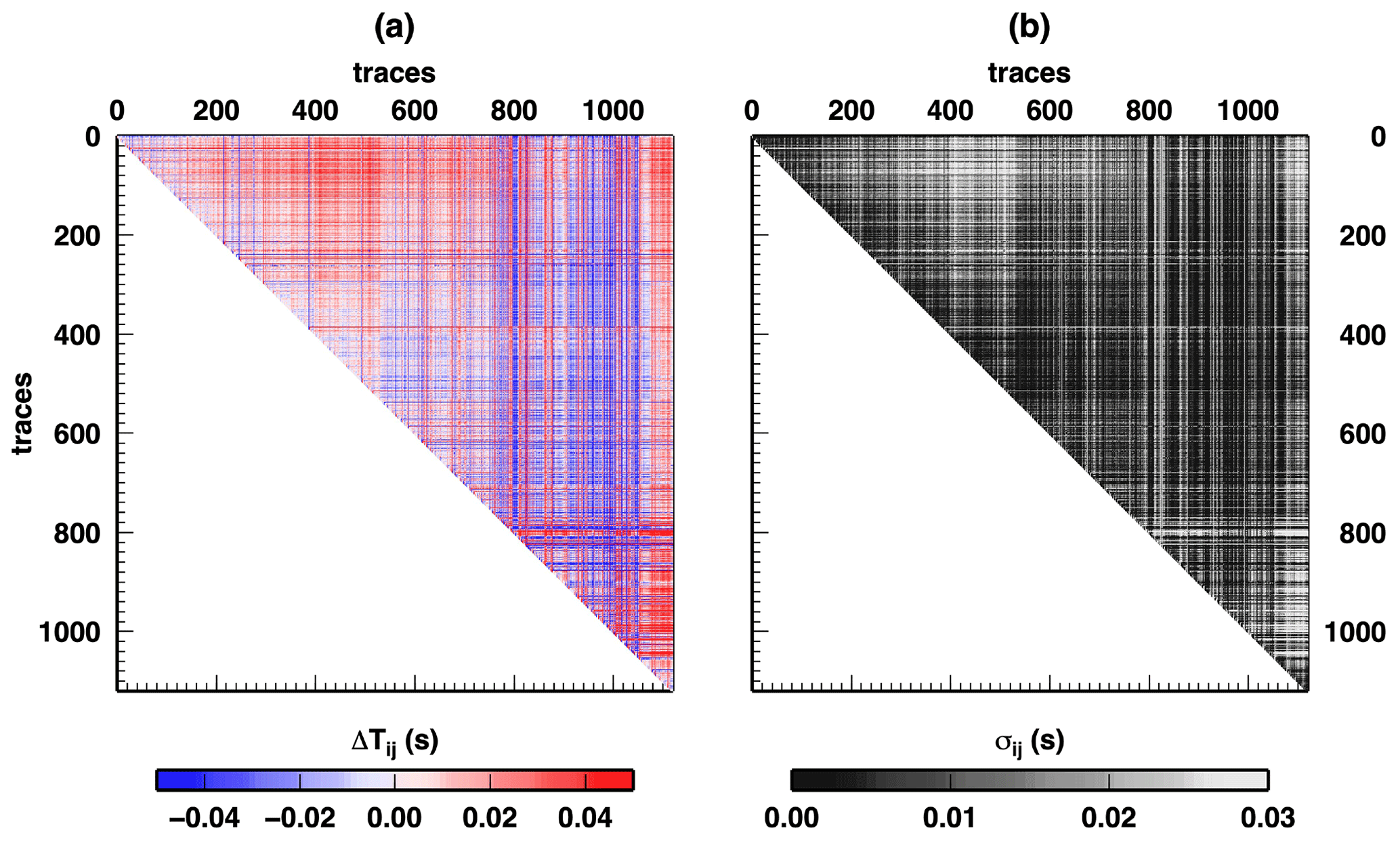
We test our novel methodology for preparing DD data with a single-station data set recorded on Katla volcano in Iceland during a 2-year monitoring experiment. We collected all the waveforms recorded by one seismic station on the volcano flank, which is far enough from a source of repeating earthquakes (i.e. all waveforms have a high degree of similarity) to be considered a pointwise seismic source. Details about the data preparation are given in Appendix B. The DD data are represented by the vector d=d_ij with $i=\mathrm{1},\mathrm{\dots },N_{\mathrm{e}}-\mathrm{1}$, $j=i+\mathrm{1},\mathrm{\dots },N_{\mathrm{e}}$, and N_e the number of events. Starting with N_e=1119 events, we obtain $N_{\mathrm{e}}\times (N_{\mathrm{e}}-\mathrm{1})/\mathrm{2}$ DD data. The total number of DD data is N_D=625 521. DD data values d_ij and uncertainties σ_ij, associated with events i and j, are reported in Fig. 3. Striking changes in DD values suggest the presence of clustering of data in time, but the exact number and positions of such clusters are not easy to define by visual inspection. Moreover, some of those changes could be due to modifications of the seismic network, in principle mapped in our DD data. In fact, our DD data depend on the origin time (OT) computed by exploiting all the recordings from the seismic network. Thus, a change in the seismic network configuration could influence the quality of seismic network detections and locations, which in turn could introduce a bias in our data as a shift in the DD value or an increase in DD uncertainties. Given the independent processes used to define each single DD datum, as a first approximation we consider our final covariance matrix of the uncertainties in the DD data ${\mathbf{C}}_{\mathit{e}}^{\ast }$ to be a 625 521×625 521 diagonal matrix, with the square of the uncertainties presented in Fig. 3b along the diagonal, omitting the correlation between uncertainties given by e.g. biases in OT determination.

Figure 3 DD data presented as a matrix of i–j pairs: (a) values and (b) uncertainties.

3 Finding data-driven time variations of rock elasticity during Katla's seismic swarm

We apply our novel methodology for the definition of the changepoints in DD data to the data set recorded on Katla volcano in Iceland during a 2-year monitoring experiment. Based on the observations of the limited dimension of the cluster with respect to the event–station distance (100 m versus 6.0 km) and the overall high similarity of the waveforms (correlation coefficient always larger than 0.9), our algorithm is able to map out which portions of the data violate our underlying hypotheses: co-located events and a constant elasticity field in time. Separating those two effects with a single station would be challenging, but here we want to illustrate in detail how the time occurrence of the changepoints is defined and compare it to other potential approaches for the definition of changepoints in DD data, namely variations in seismicity rate and waveform cross-correlation.

As shown in Fig. 1, defining changepoints for DD data using expert opinion is a dangerous task due to the limitation in the number of data available for subsequent uses. For example, seismologists could be tempted to test if using fewer data could give better images in a subsequent tomographic inversion based on pre-defined ideas about the subsurface structures. In fact, some changes in DD data are obviously present in the observations (Fig. 3, between event 550 and 1050, for example), but others are more subtle to define.

We compute the data-space exploration by running 100 independent McMC samplings, for which each chain sampled 2 million changepoint models. We discarded the first million models and collected one model every 1000 in the subsequent million models. Our final pool of models used for reconstructing the PPD is composed of 100 000 models. The full CPU time for running the algorithm is about 19 h on a 100-CPU cluster. The value of chi square decreases in the first half-million models, together with the logarithmic value of the normalizing factor in Eq. (3) (Fig. 4a). The number of changepoints reaches a stable value around 15 to 20 after 1 million models, confirming the length of the burn-in period used (Fig. 4b). The ratio between the number of event pairs not separated from any changepoint (N_F) and the total number of DD data (N_D) is also stable at around 0.2 after 1 million models, indicating that no relevant changepoint is added in the second half of the McMC sampling. It is worth noting that N_F should approximately indicate the number of DD data to be used in any subsequent analysis.

Figure 4 Evolution of some parameters along the McMC sampling. (a) Chi-square value (blue crosses) and logarithmic value of the normalizing factor in the likelihood function (red dots). (b) Number of changepoints in the sampled models (blue crosses) and ratio between the number of unaffected data (i.e. DD data for which the two events are not separated by any changepoint) and the total number of DD data, $N_{\mathrm{F}}/N_{\mathrm{D}}$ (red dots).

Looking at the full details of the PPD reconstructed from the McMC samplings, we observe the presence of long time windows completely without any changepoint (e.g. between 2011.7 and 2012.4), demonstrating the parsimoniousness of the trans-D approach: if changepoints are not supported by the data they are removed during the sampling and do not appear in the final PPD (Fig. 5e). Moreover, the most probable (relevant) changepoint (changepoint number 3 in Fig. 5e) perfectly aligns with one of the most striking changes in the DD data as shown in Fig. 5a, confirming the goodness of the approach. The distribution of the weights clearly defines the partition of the C_e(m), in which initial data (i.e. DD data related to events occurring at the initial stages of the swarm in 2011) slowly release their “connection” to later events and thus indicate that they should not be included in the subsequent analysis. From the histogram of the number of changepoints in each sampled model, we can see how the trans-D algorithm works: no fewer than 10 and no more than 20 changepoints are generally considered, even if we allow the number to increase to 100. Combining this information with the distribution of changepoints in time given in Fig. 5e, we define 11 relevant changepoints (red arrows). We again acknowledge that this number could be a subjective choice; however, looking at Fig. 5d, we see that changepoints can be “ranked” in some sense given their mean PPD weights. For example, changepoints 2, 5, and 9 have clearly associated lower weights compared to the others and should thus be considered less relevant. Our methodology does not solve all issues connected to the preparation of DD data, but, at least, it can be used to quantify the occurrence of changepoints and their importance, and such quantification can be exploited in a later stage depending on the subsequent analysis planned.

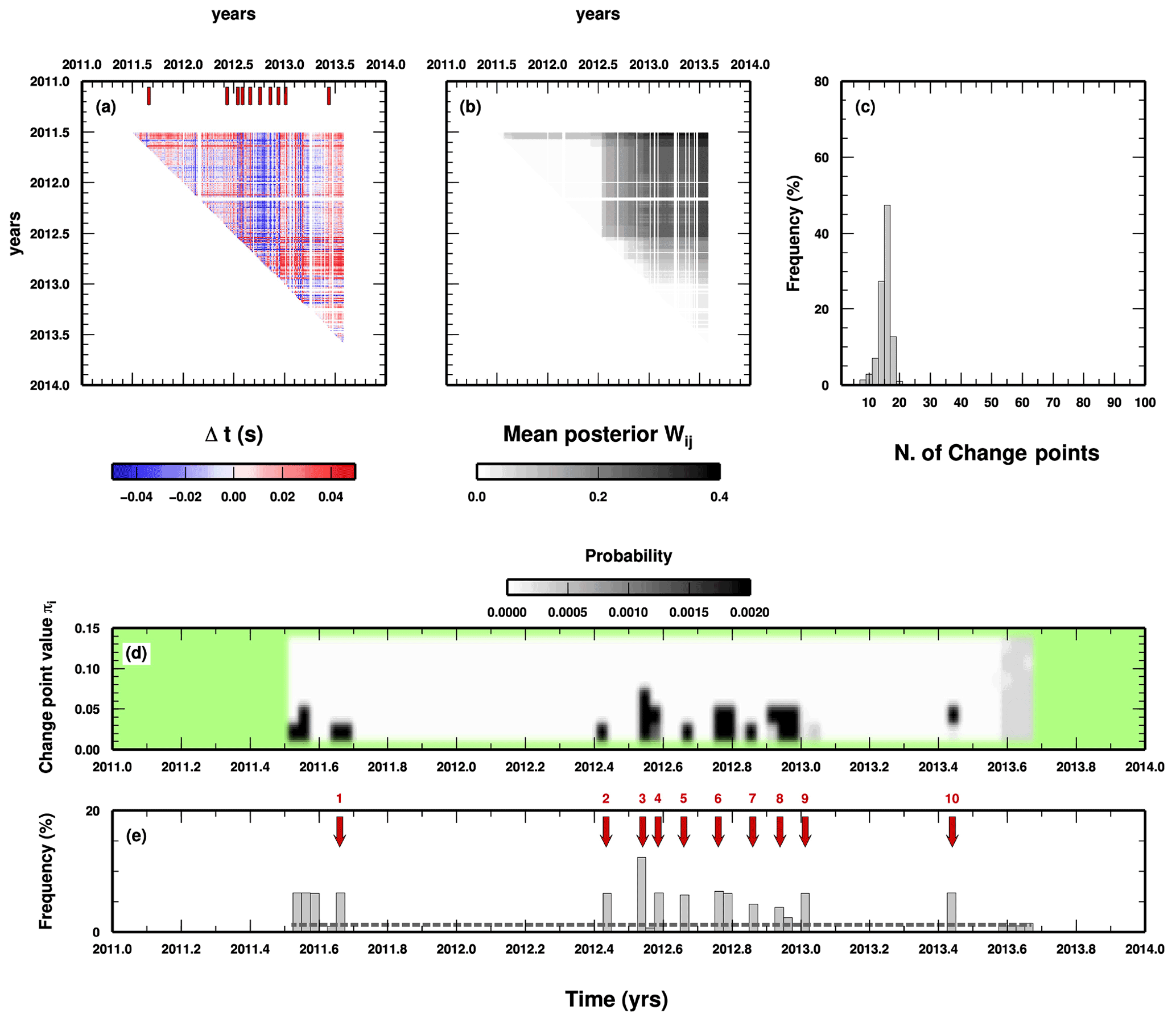
Figure 5 Results of the application of the algorithm to the Katla data set. (a) DD data and position of the most probable changepoints; see panel (e). Changepoint occurrence in time is indicated by red arrows on top. (b) Mean posterior values for the weights associated with each DD datum. (c) Histogram of the number of changepoints in the sampled models. (d) 1D marginal PPD for the values of the changepoints in time. (e) Histogram of the distribution of changepoints in time. Red arrows and numbers indicate the most probable occurrence in time for a changepoint.

We compare the occurrence in time of the resulting 10 changepoints with the cross-correlation coefficients between each event in the seismic swarm and the largest one (see Sgattoni et al., 2016a, for details). Both P-wave and S-wave cross-correlation coefficients display some degree of variability and some well-defined patterns in the time window used in this study (Fig. 6), even if we consider the fact that the smaller values are always larger than 0.9. We observe that there is no clear correlation between changepoint position in time and cross-correlation values. In mid-2011 around event 300 and early 2012 around event 700, we have two changepoints for which cross-correlation seems stable for both P and S waves. At the beginning of 2012, when the seismic network was redefined, the cross-correlation for S waves changes dramatically, whereas the change in cross-correlation for P waves is less evident, and no changepoint is found at all. Our results seem to indicate that variations in cross-correlation coefficients (for example, computed for repeating earthquakes) could indicate unrealistic variations in elasticity and could be a problematic choice for a monitoring system of the subsurface.

Figure 6 Correlation coefficients for P waves (a) and S waves (b) for each event with respect to the largest event (see Sgattoni et al., 2016a, for details). In each plot, the most probable time occurrences for the 11 relevant changepoints are also reported (yellow arrows).

We also compare the position of the retrieved changepoints with the seismicity rate, another parameter usually associated with time variations of the subsurface properties (e.g. Dou et al., 2018). In Fig. 7, we report the seismicity rate every 2 weeks. The rate of events is highly variable along the studied time window, with values ranging between a few and more than 30 events per week. The seismicity rate decreases in 2012, with some bursts up to 15 events per week in late 2012. As for the cross-correlation coefficients, the position of the retrieved changepoints does not simply correlate with the time history of the seismicity rate. We have found changepoints for which the seismicity rate is very high (2011.6) and very low (e.g. 2013.4). The most probable changepoint (changepoint number 3) occurs in a period of sustained seismicity rate that starts 5–6 weeks before. If our changepoints indicate variations of subsurface elasticity, the time history of seismicity rate should be carefully evaluated before using it for tracking elasticity changes in time. Nevertheless, we point out that the differences in the time evolution of the two indicators could be attributed to other geophysical processes, such as stress variations, which does not strictly imply elasticity variations, and we suggest that an integrated analysis could be necessary.

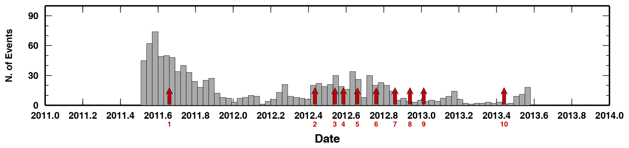
Figure 7 Comparison between the seismicity rate (grey histogram) and the time occurrences for each changepoint (red arrows and numbers).

4 Discussion

The DD data recorded on Katla volcano and the results presented here clearly indicate that time variations in elastic properties occurred between 2011 and 2014 on the southern flank of the volcanic edifice. Thus, data-driven time windows can be found using our approach to define when to apply standard DD analysis for retrieving elasticity variations, with no need to prepare the DD data following subjective choices on the paired events. With the algorithm being naturally parsimonious, there is almost no possibility of having “no DD data” (i.e. one partition per event). Changepoints are always limited in number, even if, strictly speaking, their number should be given by the user because, as final output, we have the full PPD and not just one set of best-fit changepoints. Defining the exact number of changepoints to use in subsequent analysis depends on the analysis itself. Our approach quantifies the presence and the relevance of the changepoints. Using such information could be straightforward in some cases (e.g. if we look for one most probable changepoint only) or more complex (e.g. if we also wish to appreciate correlation between changepoints, which can be measured using the PPD, such as the occurrence of a changepoint in time with respect to the occurrence of another changepoint). It is worth noticing that, in simple cases, our algorithm generally performs as expert opinion (e.g. in the case of the search for one most probable changepoint), and this confirms the overall performance of our methodology. In more complex cases, the weights associated with the changepoints should be used to classify the changepoints themselves, and this allows selecting the most relevant changepoints using quantified information.

The network of seismic stations deployed around Katla volcano changed in time. This fact has been previously indicated as a potential “bias” in the analysis of the seismic data themselves, as the location uncertainties increased after major network operations (January 2012). Our results point out that the changepoints found do not correlate with such a change in the seismic network. Being a statistical analysis, our methodology seems to be insensitive to changes in the acquisition system. Alternatively, the changes in location uncertainties may not be large enough to affect our procedure. In both cases, our approach appears to be well-suited for handling long-lived databases in which changes in the spatial distribution of observational points are likely to occur from time to time.

Finally, we investigate how our changepoints relate to more commonly used indicators of subsurface variations of elasticity, such as time series of cross-correlation coefficients and seismicity rate. In both cases, we found poor correlation between our results and the time series of the two quantities. Although this observation is not totally unexpected since the two time series are based on different seismological observables, it suggests that care should taken when investigating time variations of elasticity retrieved from methodologies based on cross-correlation and re-assessing approaches based on variations of the seismicity rate as a proxy for “rock instabilities” (Dou et al., 2018).

5 Conclusions

We developed an algorithm for defining data-driven partitions in a seismic database for a more objective definition of double-difference data. The algorithm is based on the trans-dimensional sampling of data structures, represented here as partitions of the covariance matrix. The algorithm has been tested in the case of a seismic database acquired in a volcanic setting, where subsurface variations of rock elasticity have probably occurred over a period of 2 years. Our results indicate the following:

1. trans-dimensional algorithms can be efficiently used to map data structures in the case of double-difference data, namely separating events with a number of changepoints that define time windows consistent with the underlying hypothesis (here a constant-in-time elasticity field between station and event cluster);

2. changepoints are quantitatively defined and can thus be ranked based on their relevance (i.e. weights) and probability of occurrence at a given time;

3. the results obtained are insensitive to changes in network geometry during the seismic experiment.

The applications of our algorithm are not limited to the standard preparation of DD data but could be adopted for a more complex workflow, such as separating time windows for demeaning of DD data (Roecker et al., 2021). Future development and testing will provide additional insights into the use of trans-dimensional algorithms for the exploration of the data space. For example, in this specific case, our algorithm can be applied to the joint inversion of both P-wave and S-wave databases following the approach described in Piana Agostinetti and Bodin (2018) to reconstruct a set of changepoints based on P-wave data and a set of changepoints based on S-wave data. Comparing the two sets of changepoints, “decoupled changepoints” (i.e. changepoints occurring for one set of waves and not for the other) would properly map out elasticity variations, resolving the trade-off (still existent now) between elasticity changes and changes in event locations. In fact, variations in event location would be indicated by “coupled changepoints”, i.e. changepoints occurring in both sets (Piana Agostinetti and Bodin, 2018).

Appendix A: Synthetic tests

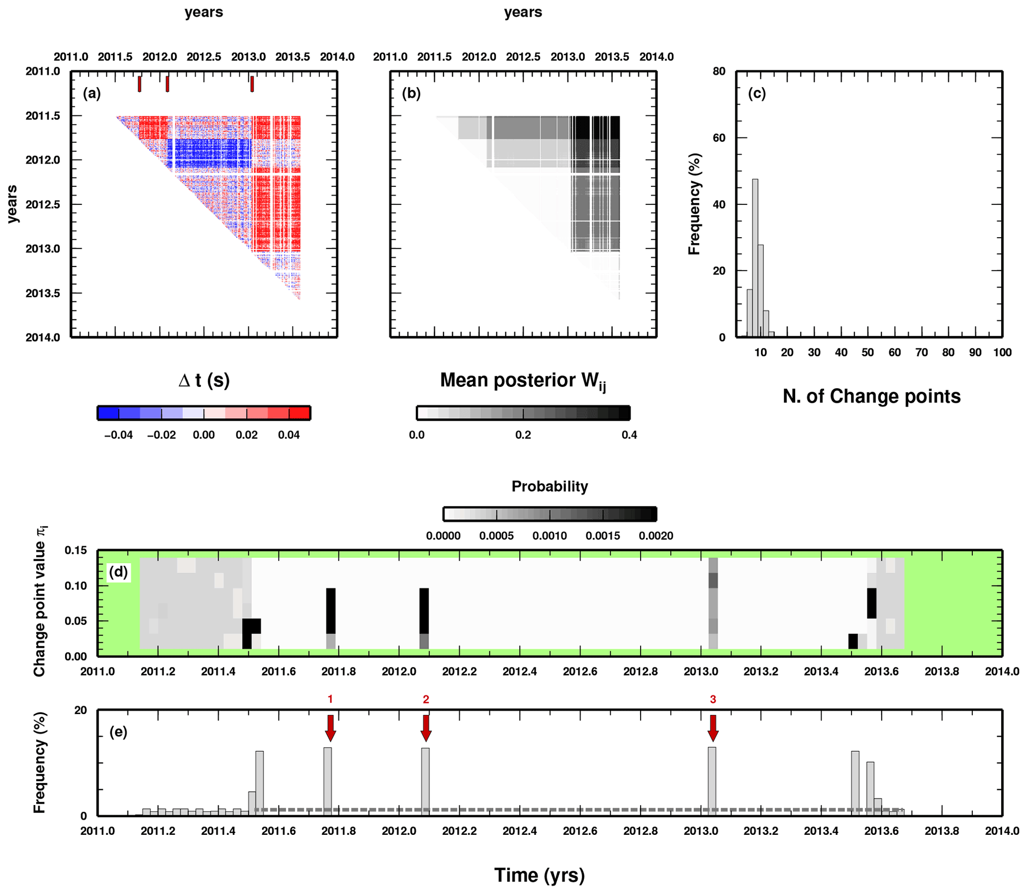
We perform two simple synthetic tests to illustrate the “parsimonious” behaviour of our trans-dimensional approach. In a first test, we make use of synthetic DD data created without imposing any changepoint in the data. Basically, the data are distributed according to the uncertainty statistics introduced in Eq. (6). Moreover, we also add a random shift to the origin time (OT) of the events to closely mimic the field measurements. OT shifts are randomly picked from a uniform distribution of ±0.02 s. Synthetic data used as input can be seen in Fig. A1a. In the second test, we introduce three changepoints in the same DD data used in the previous test. The three changepoints introduce a DD value as large as ±0.04 s for some time windows, affecting some of the event pairs, which is overimposed to the OT shift. Synthetic data used as input for this second test can be seen in Fig. A2a. The time occurrence of the three changepoints is easily recognized in Fig. A2a; however, the presence of the OT shifts introduces an additional source of noise, which seems to create fake changepoints.

In Fig. A1, we report the result of the first test. The parsimonious behaviour of our trans-dimensional approach limits the number of changepoints to the minimum (1). Such a changepoint appears to be at the very beginning of our time series of DD data (Fig. A1e), with few event pairs affected by its presence. Hence, we suggest that the occurrence of changepoints close to the boundary of the time series should be carefully evaluated due to the limited information on which their presence is based.

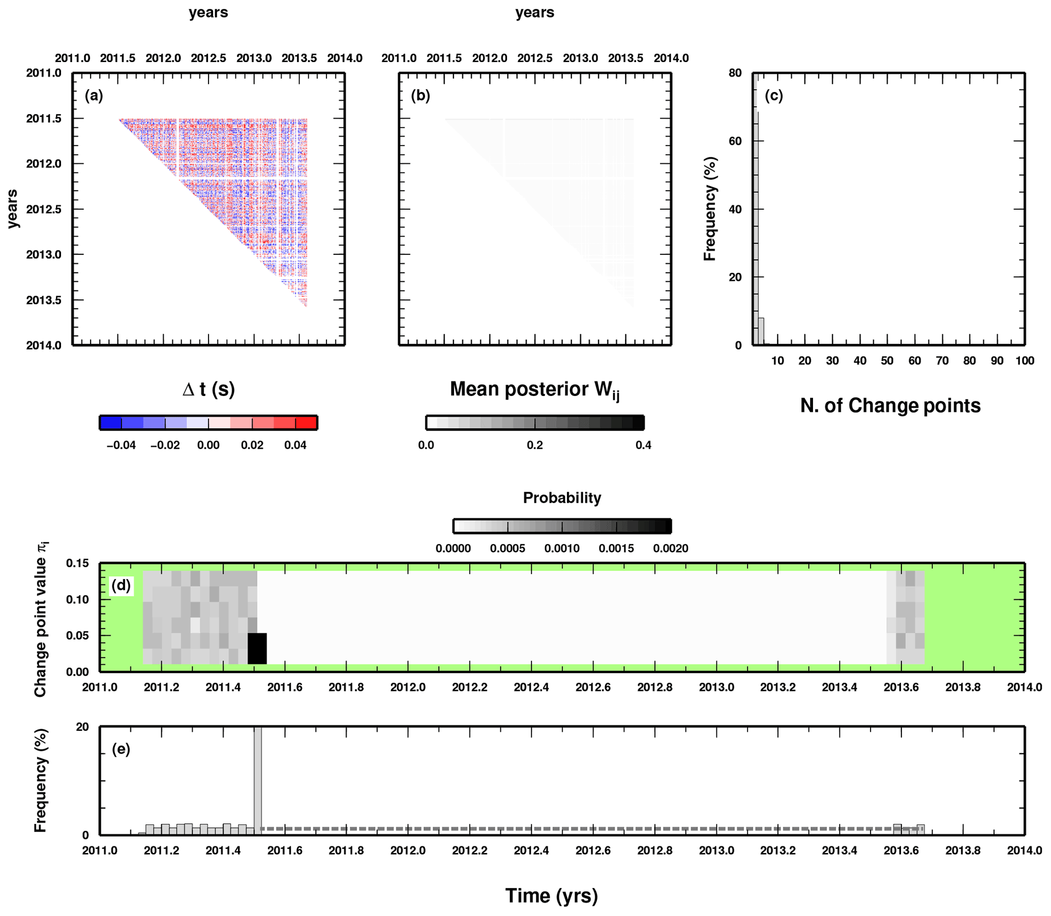
Figure A1 Results of the synthetic test wherein “observed” data have been created without changepoints. Figure details are the same as in Fig. 5. In panel (a) we show the synthetic data used as input to the algorithm.

In Fig. A2, we report the result obtained during the second test. Here, the three changepoints are clearly retrieved in the middle of our time series (Fig. A2e). However, also in this case, few additional changepoints are inserted at the beginning and at the end of the time series, reinforcing the suggestion of the first synthetic test to carefully evaluate changepoints which affect a limited number of data (in our case, changepoints occurring at the very beginning of the time interval considered here).

Figure A2 Results of the synthetic test wherein “observed” data have been created with three changepoints. Figure details are the same as in Fig. 5. In panel (a) we show the synthetic data used as input to the algorithm.

Appendix B: Data preparation

We use data from a cluster of repeating earthquakes located on the southern flank of Katla volcano (Iceland; Fig. B1a). This seismic activity initiated in July 2011 following an unrest episode of the volcano (Sgattoni et al., 2017) and continued for several years with remarkably similar waveform features over time. The cluster is located at a very shallow depth (<1 km) and consists of small-magnitude events ($\sim -\mathrm{0.5}$–1.2 ML) characterized by emergent P waves and unclear S waves, a narrowband frequency content around 3 Hz at most stations, and correlation coefficients well above 0.9 at the nearest stations during the entire sequence. The temporal behaviour is also peculiar, with a regular event rate of about six events per day during warm seasons gradually decreasing to one event every 1–2 d during cold seasons (Sgattoni et al., 2016b). Sgattoni et al. (2016a) obtained relative locations of 1141 events recorded between July 2011 and July 2013 by designing a method optimized for very small clusters that includes the effects of 3D heterogeneities and tracks uncertainties throughout the calculation. The number of relocated events depends on a selection of the best events among a total of >1800 based on thresholds on the correlation coefficient and number of detected P and S phases. The resulting size of the cluster is on the order of $\mathrm{25}\times \mathrm{50}\times \mathrm{100}$ m³ (easting, northing, depth), with estimated uncertainties on the order of a few tens of metres (Fig. B1b). Changes in the station network configuration around the cluster occurred due to technical problems, with the greater loss of data in the second part of the sequence after January 2012. This coincides with a clear increase in relative location uncertainties, which also correlates with a decrease in correlation coefficients, mainly for S phases. Other temporal changes in waveform correlation were identified by Sgattoni et al. (2016a) in August 2012 and January 2013. In this study we focus on P-wave data recorded at station ALF (part of the Icelandic Meteorological Office seismic network), which is located about 6 km away from the cluster (Fig. B1a) and is the only nearby station that was continuously operating during the entire time. The similarity of the waveforms recorded at ALF is remarkable, with correlation coefficients of the largest events above 0.99 throughout the entire period of study (Fig. B1c). To compute the DD data set, we use the origin times (OT_i) of N_e=1119 relocated events from Sgattoni et al. (2016a). We remark that the increased location uncertainties due to the network geometry change in January 2012 may affect the quality of the locations of the events and, consequently, the determination of their origin times, which is relevant for computing uncertainties in the DD data (see Sect. B1).

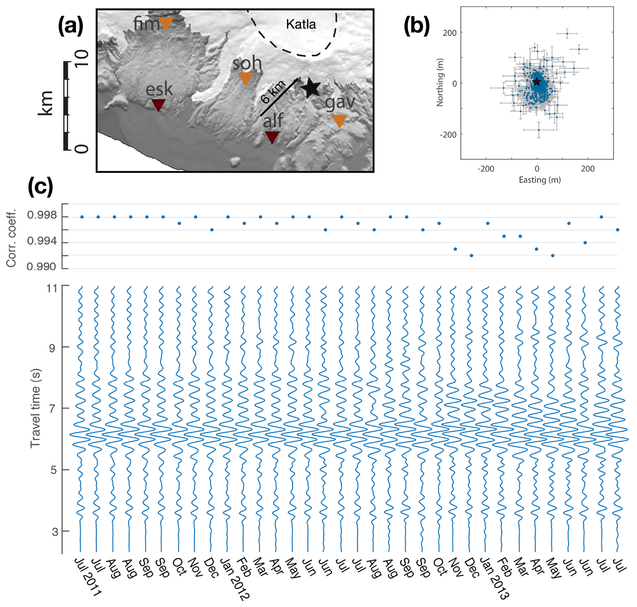
Figure B1 (a) Map of the southern flank of Katla volcano (Iceland; topography information from the National Land Survey of Iceland). The caldera rim is outlined by the black dashed line. White areas are glaciers. The star marks the location of the seismic cluster. Dark brown triangles: permanent Icelandic Meteorological Office (IMO) seismic stations. Orange triangles: temporary Uppsala University seismic stations operating between May 2011 and August 2013. (b) Relative locations (blue points) and uncertainties (± std; grey lines) from Sgattoni et al. (2016a) (c) Example waveforms of the Z component recorded at station ALF throughout the entire period investigated and correlation coefficients of the P waves with respect to the master event used for the relative locations shown in (b). Panels (a) and (b) have been modified from Sgattoni et al. (2016a). Panel (c) has been modified from Sgattoni et al. (2016b).

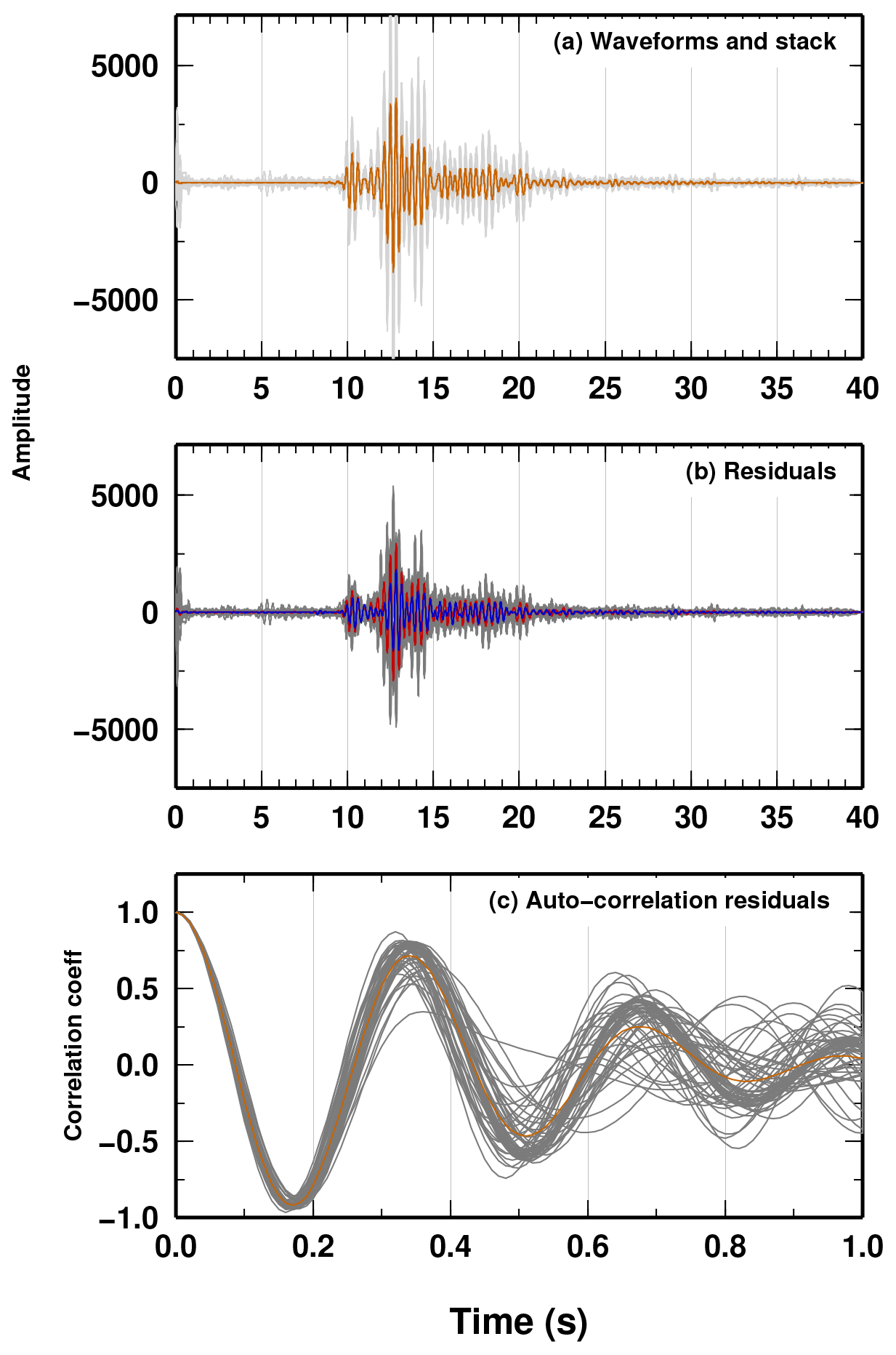
Figure B2 (a) Original waveforms w_i(t) (grey lines) and their stack, called “beam waveform” b(t) (orange line). (b) Residual of each single waveform r_i(t) (grey lines) with respect to the beam waveform. As a reference, the residual for the first (last) trace is shown as a blue (red) line. (c) Autocorrelation of the single residuals (grey line) and averaged value of the autocorrelation c(t) (orange line).

B1 Data uncertainties from full waveform investigation

To apply our novel Bayesian approach, we need to estimate a covariance matrix of the uncertainties in the DD data. Having an origin time OT_i for the ith event (given by the location obtained in Sgattoni et al., 2016a, using the full seismic network), we derive the DD data and their uncertainties directly by comparing the raw waveforms and finding the absolute delays between each pair of events. From the absolute delays of the P arrivals, the subtraction of the time differences in the OTs of two events gives the DD datum for each pair. We estimate the absolute time delay between two events following the Bayesian approach described in Piana Agostinetti and Martini (2019). Briefly, (a) we collected a 20 s record of each event w_i(t) with $i=\mathrm{1},\mathrm{\dots },N_{\mathrm{e}}$, centred on the approximate P-wave arrival time; (b) we stack all the waveforms of the events and obtain the so-called beam waveform $b\left(t\right)=\frac{\mathrm{1}}{N_{\mathrm{e}}}{\sum }_i{w}_i\left(t\right)$ (Fig. B2a); (c) from the beam waveform, we compute the residuals for each event $r_i\left(t\right)=b\left(t\right)-w_i\left(t\right)$ (Fig. B2b); (d) event residuals define a standard deviation function $\mathit{\sigma }\left(t\right)=\frac{\mathrm{1}}{N_{\mathrm{e}}}\sqrt{{\sum }_i{r}_i(t{)}^{\mathrm{2}}}$ for the 20 s record; (e) event residuals are also autocorrelated to obtain an averaged autocorrelation function c(t). The standard deviation and the autocorrelation function are used to define a covariance matrix Σ_e,w (the same for all the waveforms; Piana Agostinetti and Malinverno, 2018) using the equation

$$\begin{array}{}\text{(B1)}& {\displaystyle }{\displaystyle }{\mathbf{\Sigma }}_{\mathbf{e},\mathbf{w}}=\mathbf{S}\mathbf{R}\mathbf{S},\end{array}$$

where Σ_e,w is the covariance matrix of the waveform uncertainties, S is a diagonal matrix containing the standard deviation σ(t) computed from the residuals, and R is a symmetric Toeplitz matrix whose rows and columns contain the autocorrelation function c(t) with t=0 on the diagonal. In this way, we reconstruct a full covariance matrix, which can be used to obtain realistic uncertainty estimates for our DD data. It is noteworthy that the use of a diagonal covariance matrix instead of the full Σ_e,w covariance matrix would risk underestimating the uncertainties, biassing the subsequent analysis for defining the DD time windows. Having the uncertainty model for the waveforms for each pair of waveforms associated with ith and jth events we perform a Markov chain Monte Carlo sampling (Mosegaard and Tarantola, 1995) to reconstruct the PPD of the time shift t_ij between the two waveforms. Following Sgattoni et al. (2016a), we use a 1 s long time window to compute the likelihood of the waveforms, centred on the approximate P-wave arrival time. From the reconstructed PPD, we use the mean posterior value of the time shift ${\stackrel{\mathrm{̃}}{t}}_{ij}$, its standard deviation ${\stackrel{\mathrm{̃}}{\mathit{\sigma }}}_{ij}$, and the origin times OT_i to produce the DD data, namely $d_{ij}={\stackrel{\mathrm{̃}}{t}}_{ij}-({\text{OT}}_j-{\text{OT}}_i)$ and ${\mathit{\sigma }}_{ij}={\stackrel{\mathrm{̃}}{\mathit{\sigma }}}_{ij}$, with $i=\mathrm{1},\mathrm{\dots },N_{\mathrm{e}}-\mathrm{1}$, $j=i+\mathrm{1},\mathrm{\dots },N_{\mathrm{e}}$, and j>i.