Sedimentary basins of the eastern Asia Arctic zone: new details on their structure revealed by decompensative gravity anomalies

In the present study, the structure of sedimentary basins in the eastern Asia Arctic zone is analysed by employing the approach based on decompensative gravity anomalies. Two obtained models, differing in their initial conditions, provide thickness and density of sediments in the study area. They demonstrate essentially new details on the structure, shape, and density of the sedimentary basins. Significant changes in the sedimentary thickness and the depo-centre location have been found for the Anadyr Basin in its continental part. Also, new details on the sedimentary thickness distribution have been revealed for the central part of the Penzhin and Pustorets basins; for the latter, the new location of the depo-centre has been identified. The new model agrees well with the seismic data on the sedimentary thickness for the offshore part of the Chauna Basin confirming that the method is robust. The most significant lateral redistribution of the thickness has been found for the Lower Cretaceous coal-bearing strata in the northern part of the Zyryanka Basin, where the connection of two coal-bearing zones, which was not previously mapped, has been identified. Also, the new details on the sedimentary thickness distribution have been discovered for the Primorsk Basin. Therefore, the new results substantially improve our knowledge about the region, since previous geological and geophysical studies were unsystematic, sparse, and limited in depth. Thus, the implementation of the decompensative gravity anomalies approach provides a better understanding of the evolution of the sedimentary basins and the obtained results can be used for planning future detailed studies in the area.

1 Introduction

In this study we analyse the structure of sedimentary basins in the north-eastern part of Asia, including the Asia Arctic zone and the adjacent areas of the Arctic Ocean, by employing the approach based on the decompensative gravity anomalies (Haeger and Kaban, 2019; Kaban et al., 2021a, b). This method is employed together with one of the most recent gravity field models EIGEN6-c4 (Förste et al., 2014).

The structure and density of sedimentary basins represent a natural record of former tectonic activity. Therefore, knowledge of the sedimentary structure can provide a basis for understanding the history and formation of various geological structures. This information can be used in various studies in geology and Earth history, geodynamics, oceanology, paleogeography, etc. Furthermore, these results are important for numerous practical applications, particularly for mineral deposit prospecting and the development of the necessary infrastructure, including pipelines and railways. This is the key issue for the economic development of such regions as the Asia Arctic zone.

Up to now, the north-eastern part of Asia remains one of the least studied areas in the world, due to the inaccessibility of this territory, its rigorous climate, and low habitability. The systematic geographical and geological exploration of this region began only less than 100 years ago. One of the first effective scientific expeditions into the “middle of nowhere” was the expedition of Sergei Obruchev in 1926–1930, when one of the last mapped mountain ridges in Asia – the Chersky Ridge – was discovered. A lot of geological studies were conducted later in the north-eastern Asia region, in particular mineral prospecting (ore, carbohydrates, coal, etc.) (e.g. Sitnikov, 2017; Morozov, 2001). However, most of these were focused on surface geology, while the area is still poorly studied by geophysical (first of all, seismic) methods. Thus, the deep structure of many sedimentary basins remains unclear, and the information on their development is often based on very generalized and sometimes outdated hypotheses. Furthermore, for some particular areas within the eastern Asia Arctic zone, like Chukotka, there exist contradicting hypotheses about their origin due to insufficient knowledge about their structure (Morozov, 2001). Therefore, detailed models of these structures obtained with modern geological and geophysical data and methods can help to justify some of the suggested hypotheses.

The lithosphere in this region represents a complex combination of different structures that developed generally from the Jurassic to the Quaternary during several periods of intense tectonic activity and relatively quiet periods of sedimentation. Three large tectonic elements with different structural patterns and different history can be distinguished within the study area: the Verhkoyansk (Verkhoyansk–Chukotka) orogen, the Koryak orogen, and the Okhotsk–Chukotka volcanogenic belt.

The gravity field is often used to study sedimentary basins because sediments normally have a large density contrast relative to surrounding consolidated rocks (e.g. Langenheim and Jachens, 1996; Jachens and Moring, 1990; Ebbing et al., 2007; Kaban et al., 2021a, b). On the other hand, the gravity data usually have complete and homogeneous data coverage, while seismic determinations are limited to seismic profiles or even single points. The recent satellite missions have provided data even for the continental areas not covered by terrestrial or airborne prospecting (e.g. Förste et al., 2014). Typically, the Bouguer or isostatic gravity anomalies are employed for studying sediments. The isostatic anomalies are considered more appropriate because they are refined to some extent from the effect of deep density variations (e.g. of the Moho undulations), which are dominated in the Bouguer anomalies (e.g. Simpson et al., 1986; Blakely, 1995). Consequently, the isostatic gravity anomalies have been extensively used for these purposes (e.g. Jachens and Moring, 1990; Langenheim and Jachens, 1996; Ebbing et al., 2007).

However, this method works correctly only for small-scale basins like the Los Angeles Basin (Langenheim and Jachens, 1996) or for narrow basins (e.g. in Nevada; Jachens and Moring, 1990). For larger basins, the gravity effect of sediments is significantly reduced due to isostatic compensation (e.g. Cordell et al., 1991). For wide basins (≈300–400 km and more) this reduction may even exceed 1 order of magnitude (Kaban et al., 2021a). Zorin et al. (1985) and Cordell et al. (1991) suggested recovering the full effect of sediments by computing decompensative gravity anomalies. Afterwards, this method was successfully employed for studying the upper crust in many regions (Cordell et al., 1991; Hildenbrand et al., 1996; Zorin et al., 1993; Wilson et al., 2005). Recently, this approach has been improved to account for elastic deformations of the lithosphere via its effective elastic plate thickness (EET) (Kaban et al. 2017; Haeger and Kaban, 2019).

For implementing the method, we use the strategy, which was formulated in Kaban et al. (2021b) for studying the southern part of the East European platform. In the first step, the isostatic anomalies of the gravity field are estimated. Then, we compute the decompensative correction for these anomalies and use it for improvement of the initial model of the sedimentary cover.

Figure 1 Topography and bathymetry of the study area. Dark grey contours represent positions of sedimentary basins. The basin captions are in bold. The dashed line indicates the OCVB continental borders. Here and in all subsequent maps the following abbreviations are used to denote the following sedimentary basins: L-MB – Laptev–Moma Basin; ZB – Zyryanka Basin; PrB – Primorsk Basin; TB – Tastakh Basin; ChB – Chauna Basin; PeB – Penzhin Basin; PB – Pustorets Basin; AB – Anadyr Basin.

2 Study area

2.1 An overview of the geological and tectonic history

The study area represents a part of north-eastern Asia and spans 135 to 190^∘ E and 65 to 74^∘ N. The topography and bathymetry of the region with main geological structures are shown in Fig. 1. Most of the continental area is represented by the Verkhoyansk orogen – a large system of mountain ridges that were formed during Cimmerian times. The orogen is mostly dominated by the middle and late Paleozoic (Carboniferous and Permian) to Mesozoic (Triassic and Late Jurassic) terrigenous rocks accumulated in the passive margin conditions of the Siberian Platform and deformed then during the collision between the East Siberian and East Arctic continental lithospheric plates (Sitnikov and Sleptsova, 2020) and later – in the collision of the Pacific and the Chukotka plates. In the Late Mesozoic, continental magmatism led to the upwelling of granitic and granodiorite batholiths, forming the mountain ridges. The largest ridges forming the orogeny of this age in the studied region are the Chersky and Suntar–Khayata ridges, as well as the Near-Kolyma uplifts (a part of the large Kolyma–Omolon superterrain). The eastern part of the region includes such large mountain ridges as the Kolyma Mountains, Chukotka Mountains, and Koryak Mountains (the Anadyr–Koryak folded system). In the Late Cenozoic, new deformations occurred, complicating the Mesozoic tectonic structure of the orogen. In the central part of the region, the arched block rose, while the northern parts of the region subsided, and a thin cover of the Cenozoic sediments was formed there. In the southern part of the sea shelf, marine sediments accumulated.

The northern part of the territory is bounded by the Arctic Ocean shelf of the Laptev Sea, the East Siberian Sea, and the Chukchi Sea.

Continental sedimentary basins of the studied territory formed as

1. intermontane depressions of the Mesozoic basement

2. basins filling new Cenozoic rifts (Laptev–Moma Basin system)

3. continental margins of the sea shelf.

The Okhotsk–Chukotka volcanic belt (OCVB), located in the eastern part of the region, extends along the north coast of the Sea of Okhotsk for about 3000 km and then to the north-east in the Chukotsk Peninsula. The dashed line in Fig. 1 indicates the OCVB continental borders. In the south-west, the Okhotsk segment of the belt is 1400 km long and is different in some ways from the Chukotka segment, which is 1600 km long. The belt is composed of subaerial volcanic rocks, in particular of the rhyolites, andesites, and basalts, forming the lava cover. The sedimentary rocks forming the OCVB structures are partly terrigenous, partly volcano–tuff–terrigenous, while the volcanoclastic rocks are much less abundant. Most of these rocks are of late Early Cretaceous–Late Cretaceous age and younger. The eastern part of the Kolyma Mountains and southern part of the Chukotka Mountains is chiefly made up of the Cretaceous volcanogenic rocks related to the OCVB formation.

2.2 Sedimentary basins, their origin, and structure

Most of the sedimentary basins on the continental part are characterized by low thickness mainly due to a relatively short period of sedimentation in the passive continental margins or in the intermontane depressions (Sitnikov et al., 2017). The deepest sedimentary basins in the area are related to the grabens continuing to the Arctic shelf and formed on the Late Mesozoic and Cenozoic basement. In this study, we analyse relatively deep (more than 0.5 km) and most extended sedimentary basins in the continental part of the region and on the sea shelf. These basins are related to different stages of the geological evolution of the region and were formed during different periods (from the middle and Late Mesozoic to the Cenozoic).

First of all, we consider the easternmost continental branches of the Laptev–Moma Basin (LMB), which is a rift-related structure represented by the grabens that appeared in the Cenozoic with the limnic deposits of the Oligocene–middle Miocene. Over them, the alluvial–proluvial sediments of the upper Miocene–Holocene were then accumulated. This structure is a part of the larger basin, which continues northward from the continent into the Laptev Sea shelf (the south-west Laptev Basin), which also includes the Lena River delta. In the continental part and the nearest shelf, the Shiroston and Ust'–Yana grabens can be also distinguished in the study region (Andieva, 2008).

The Zyryanka Basin is an internal depression within the Kolyma massive. Geographically it comprises the valleys of the Indigirka and Kolyma rivers. This large depression formed in the final stages of the Verkhoyansk Mesozoic orogeny. Some studies initially assumed that the Zyranka depression is a foredeep but not an intermontane depression (Koporulin, 1979). The sediments filling the depression are of the Upper Jurassic, Cretaceous, and Paleogene to Quaternary ages (Clarke, 1988). The basement of the depression is irregular and exposed in several locations. In the post orogenic stage, during the Early Cretaceous, the strata of the continental limnic molasses (represented by sandstones, conglomerates, etc.) with thick coal beds were accumulated. The nearest Moma (Moma–Selennyakh) depression is located to the south of the Ilin'–Taas inversion uplift, separating it from the Zyryanka depression. Initially, these two depressions formed on the basis of the large Moma–Zyryanka rift system (Grachev et al., 1970); later a significant difference was discovered in the sedimentary strata composing the upper part of the Moma depression (with higher metamorphism compared to the Zyryanka depression). The Lower Cretaceous sediments in the Moma Basin are represented only by Neocomian to Aptian strata in isolated troughs with a maximum thickness of 3 km. The Cenozoic (Paleogene to Quaternary) sedimentary thickness is relatively insignificant.

The Primorsk Basin, using the name given by Drachev (2011), or the Lower Kolyma Basin, according to Sitnikov and Sleptsova (2020), is located mainly in the East Siberian (or Lower Kolyma) lowland in the downstream part of the Indigirka, Alazeya, and Kolyma rivers; however, its northern part is located offshore on the Arctic Ocean shelf (the basin shape can be seen in Fig. 1). Its folded basement is represented by the Polousnensky folded structure on its western part and by the South Anyui suture in its eastern part. The Primorsk Lowland is covered by thick Neogene–Quaternary deposits, which complicate the study of its structure. Therefore, the thickness of the sedimentary cover of this basin (of Mesozoic to Cenozoic to Quaternary age) has been differently determined in many existing studies.

The Tastakh (or Tas-Takh) Basin is located west of the Primorsk Basin and separated from it by the Khroma height. Pavlova (2020) suggests that the Tastakh Basin is the marginal part of the larger depression mostly located offshore. From the middle of the 1980s, it was studied by geological, gravimetric, and aeromagnetic surveys of various scales. Similarly to previously discussed basins, the sedimentary cover includes Upper Mesozoic and Cenozoic (Paleogene–Neogene–Quaternary) strata. The sedimentary thickness and structure in this basin are still poorly studied. Sitnikov and Sleptsova (2020) referred to the Primorsk and Tastakh basins as the structures formed due to lithospheric deformations during the Mesozoic subduction. In the deepest parts of these depressions, the relics of the transitional types of the crust have been preserved. The edges of the depressions later evolved as autochthonous structures, both representing geologically different types than the initial deformations.

The Chauna Basin, located at the western border of the New Siberian–Chukotka orogen, appeared in the Early Cretaceous. Gresov and Yatsuk (2020) regarded this depression as a part of the larger Ayon Basin, located offshore and continuing to the continent. Both the Chauna and Ayon depressions were formed as grabens that appeared in the early Paleogene. However, in other studies, the Chauna Basin is regarded as the larger structure that includes the Ayon Basin (Drachev, 2011; Shipilov and Lobkovsky, 2019; Sitnikov and Sleptsova, 2020). The basin, overlying the folded Early Mesozoic basement, is filled with the Upper Jurassic and Lower Cretaceous coarse–detrital molasses and volcanic rocks (andesites and rhyolites), 2.2 to 2.5 km thick, according to the marine seismic survey (Gresov and Yatsuk, 2020).

The Penzhin Basin is located in the Olyutor–Kamchatka belt of Cenozoic folding. This basin is similar in age and composition of the sedimentary and volcanic rocks to other two basins on the eastern coast of Kamchatka (Il'Pin and Olyutor). The clastic and volcanic rocks of Late Cretaceous and Cenozoic age form the section of these basins (Ivanov, 1985; Clarke, 1988). In some earlier studies (e.g. Tilman et al., 1969) only the upper structural section is considered. The basement of the Penzhin Basin includes the Paleozoic and Mesozoic rocks formed before the pre-Aptian Cretaceous time. The sedimentary fill is of the Late Cretaceous to Cenozoic age.

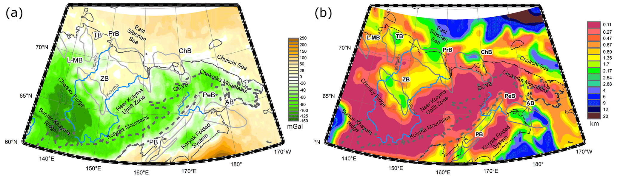
Figure 2 (a) Initial Bouguer gravity data. (b) Thickness of sediments according to the initial model.

The Pustorets Basin is another depression on the west coast of northern Kamchatka, extending offshore. It is 450 km long and 50–100 km wide, located on the north-west margin of the Olyutor–Kamchatka, which bounds the Anadyr–Koryak fold system. The folded basement of this basin consists of the Cretaceous rocks (corresponding to nearly all stages of the Cretaceous period) with the deepest part related to the Aptian–Albian time metamorphosed to greenschist facies and intruded by granite and gabbro in the south-east border. The sediments filling the basin are of Cenozoic age. The top part of the Cenozoic section is represented by the Oligocene–Miocene sediments; most of them are sandstones and conglomerates. Their thickness is up to 2500 m. The Pustorets Basin is bounded on the north-west by the Penzhin–Parapol deep fault and on the south-east by the Vyven deep fault. Within the basin, there exist several highs and lows, which follow the trend of the basin. In the south-west along the shore of the Penzhin Gulf, the Kinkil high, which is 240 km long and about 40 km wide, is located. One can identify three structural sections in this high. The lower one consists of the Paleocene–Eocene sedimentary rocks, the second one is comprised of the Eocene–Oligocene volcanic rocks, and the third section is locally distributed Neogene sediments.

The Anadyr Basin is located at the easternmost part of the study area. It was formed during the Late Mesozoic and Early Cenozoic during the collision of the South Anyui ocean in the convergence zones of different ages along the Asia continental margin and the Pacific Ocean plate. The folded basement of the basin was formed during the Late Cretaceous (Albian–Cenomanian) orogeny. The evolution history of the sedimentary cover can be divided into three periods: (1) sediment accumulation during the passive continental margin phase (Late Cretaceous–early Eocene); (2) sediment accumulation in middle Eocene–Oligocene during the extension and rift formation in the northern part of the basin and compression in its southern part due to the northward movement of the foredeep before the Koryak accretion orogeny; (3) Miocene sediment accumulation in the conditions of continental rifting (Antipov et al., 2008).

The position of the main sedimentary basins in the study area is shown in Fig. 1. This scheme is chiefly based on (Clarke, 1988; Drachev, 2016, 2011) and on some other publications mentioned above. More details on the structure of the analysed basins will be presented in the Discussion section with the obtained results.

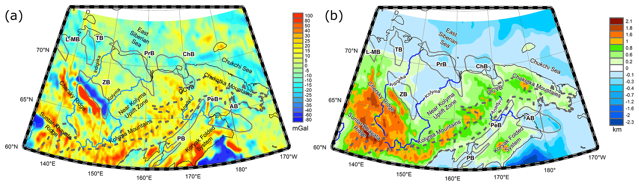
Figure 3 (a) Residual gravity anomalies. (b) Adjusted topography representing a unified surface load with the standard density of topography (2.67 g/cm³, Eq. 2).

3 Method

As was mentioned above, in the first stage we compute the isostatic gravity anomalies. By applying this correction, it is possible to remove the effect of deep density anomalies compensating the near-surface load (chiefly topography) (e.g. Simpson et al., 1986). This correction is especially useful when we have only a little knowledge about deep structures of the lithosphere. In this case, it is just assumed that the near-surface load is compensated for according to a plausible isostatic compensation scheme. In the spectral domain, the isostatic correction is estimated using the following equation (Kaban et al., 2016, 2017):

$$\begin{array}{}\text{(1)}& \begin{array}{rl}& \mathrm{\Delta }{g}_{\mathrm{ic}}\left(k_x,k_y\right)=G_{\mathrm{is}}\left(k_x,k_y\right)\cdot t_{\text{adj}}\left(k_x,k_y\right)\\ & =-\mathrm{2}\mathit{\pi }G\mathit{\rho }\cdot C\cdot \exp \left(-k\cdot M\right)\cdot t_{\mathrm{adj}}\left(k_x,k_y\right),\end{array}\end{array}$$

where $k=\sqrt{k_x^{\mathrm{2}}+k_y^{\mathrm{2}}}$ is the wavenumber, $k_x=\mathrm{2}\mathit{\pi }/{\mathit{\lambda }}_x$ and $k_y=\mathrm{2}\mathit{\pi }/{\mathit{\lambda }}_y$, M is the depth to the Moho, and G is the gravitational constant. G_is(k_x,k_y) is the Green's function (its introduction is explained below). t_adj is the adjusted topography, which is introduced to equalize the bathymetry (t_b) and topography variations as well as the initial density variations in sediments for the constant density of the topography ρ:

$$\begin{array}{}\text{(2)}& t_{\text{adj}}=t_{\mathrm{b}}-{\displaystyle \frac{{\mathit{\rho }}_{\mathrm{w}}}{\mathit{\rho }}}{t}_{\mathrm{b}}-{\displaystyle \frac{\mathit{\rho }-{\mathit{\rho }}_{\mathrm{s}}}{\mathit{\rho }}}{t}_{\mathrm{s}},\end{array}$$

where t_s and ρ_s are the thickness and vertically averaged density of sediments from the initial model and ρ_w=1.03 g/cm³ is the water density. In the continental area, the second term in Eq. (2) is omitted.

It has been demonstrated that the main parameters, which control the style of isostatic compensation, are the average compensation depth (usually associated with the depth to the Moho) and elastic support of the surface load by the lithosphere. The parameter C determines the amount of the elastic support (C=1 for the local compensation) and depends on the EET (T_e) and wavenumber (Turcotte and Schubert, 1982):

$$\begin{array}{}\text{(3)}& C=\mathrm{\Delta }\mathit{\rho }g/(k^{\mathrm{4}}D+\mathrm{\Delta }\mathit{\rho }g),\end{array}$$

where $D={\mathrm{ET}}_{\mathrm{e}}^{\mathrm{3}}/\left[\mathrm{12}\left(\mathrm{1}-v^{\mathrm{2}}\right)\right]$ is the flexural rigidity, v is the Poisson ratio, E is the Young modulus, Δρ is the average density difference between topography and the upper mantle, and g is the gravitational acceleration.

We use a Green's function method (Wienecke et al., 2007; Braitenberg et al., 2002; Dill et al., 2015) instead of a direct application of Eq. (1) in the spectral domain, since the direct application is impossible in the case of variable depth to the Moho and EET. The above authors demonstrated that this approach is appropriate in this case. The isostatic correction is estimated in a sliding window as a convolution of the adjusted topography with the Green's functions $G_{\text{is}}\left(x,y,M,T_{\mathrm{e}}\right)$ for corresponding M(x₀,y₀) and EET (T_e(x₀,y₀)). Then, the isostatic anomalies are calculated as follows:

$$\begin{array}{}\text{(4)}& \begin{array}{rl}& \mathrm{\Delta }{g}_{\mathrm{i}}\left(x_{\mathrm{0}},y_{\mathrm{0}}\right)=\mathrm{\Delta }{g}_{\text{b}}\left(x_{\mathrm{0}},y_{\mathrm{0}}\right)+\underset{-\mathrm{1250}\mathrm{km}}{\overset{\mathrm{1250}\mathrm{km}}{\iint }}{t}_{\text{adj}}\left(x_{\mathrm{0}}+x,y_{\mathrm{0}}+y\right)\\ & \times G_{\text{is}}\left(x,y,M(x_{\mathrm{0}},y_{\mathrm{0}}),T_{\mathrm{e}}(x_{\mathrm{0}},y_{\mathrm{0}})\right)\mathrm{d}x\mathrm{d}y,\end{array}\end{array}$$

where Δg_b(x,y) is the Bouguer gravity anomaly. The radius of the sliding window is extended to 1250 km to avoid boundary effects (Kaban et al., 2021a, b).

In the second stage, the decompensative correction (Δg_dc) is calculated as follows (Kaban et al., 2017):

$$\begin{array}{}\text{(5)}& \mathrm{\Delta }{g}_{\text{dc}}\left(k_x,k_y\right)={\displaystyle \frac{\mathrm{1}}{\exp \left(k\cdot M\right)/C-\mathrm{1}}}\mathrm{\Delta }{g}_{\text{i}}\left(k_x,k_y\right),\end{array}$$

where Δg_i are the isostatic anomalies. By applying this correction, it is possible to reduce the effects of compensation of the unknown density anomalies in the upper crust, which are still missing in the initial model. Otherwise the total effect of the upper-crust anomalies and their compensation tends to zero already for the basins with a horizontal size of several hundred kilometres or more (e.g. Kaban et al., 2021a).

Unfortunately, the decompensative correction increases to infinity with increasing the wavelength. Following Cordell et al. (1991) we reduce it after a predefined wavelength (λ₀=1500 km) (Kaban et al., 2017, 2021a). This restriction does not bias the result because it is assumed that wide basins are already included in the initial model. Like for the isostatic anomalies, we apply the Green's function method to estimate the decompensative correction. A sum of the isostatic anomalies and this correction give the decompensative gravity anomalies.

4 Computation of the isostatic and decompensative gravity anomalies

4.1 Initial data

As the initial data, in this study we use the Bouguer gravity anomalies, topography, initial model of sediments (thickness and vertically averaged density), EET of the lithosphere, and depth to the Moho. For calculations, all the data have been converted to the orthographic projection with the resolution 10×10 km.

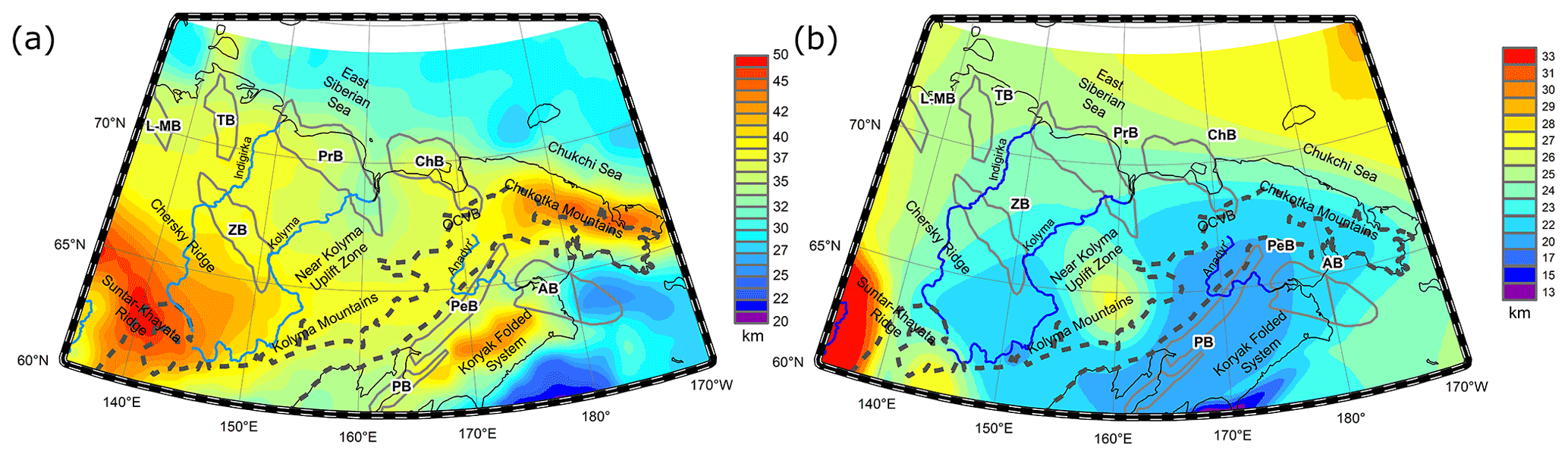
Figure 4 (a) Depth to the Moho from the sea level. (b) EET of the lithosphere.

The observed gravity field (Fig. 2a) is based on the EIGEN-6c4 model (Förste et al., 2014) that represents a combination of the recent satellite missions and surface and airborne observations. The maximal resolution is 2190 spherical harmonics degrees/order ($\approx {\mathrm{5}}^{\prime }\times {\mathrm{5}}^{\prime }$ in space); however the actual resolution depends on available surface observations. It is important that up to a resolution of approximately 70 km, this field is based on the satellite data only (Förste et al., 2014), which guarantees complete and homogeneous coverage sufficient for the present study. The topography/bathymetry is represented by the downscaled ETOPO-1 model (Amante and Eakins, 2008). For computation of the Bouguer anomalies, the topography density is assumed to be 2.67 g/cm³ and for the water it is assume to be −1.03 g/cm³ (−1.64 g/cm³ relative to the standard density of the uppermost layer). The gravity effect of the topography/bathymetry has been calculated within the radius 333.6 km (3^∘) based on the initial topography/bathymetry grids. The increase in this radius would produce only long-wavelength anomalies, which are not considered in the paper as described above.

The initial thickness of sediments is presented in Fig. 2b. For the oceans, we employed a recent high-resolution global compilation of Straume et al. (2019). For the initial densities, we used a density–depth relation for typical offshore basins from Mooney and Kaban (2010). For the continents, the data of Stolk et al. (2013) have been implemented west of 150^∘ E and for the eastern part from Kaban (2001). These papers also provide vertically averaged densities for each point of the grid. The gravity effect of the initial model of sediments is additionally separated from the Bouguer anomalies. The final residual anomalies are shown in Fig. 3a.

Based on these data, we have also estimated the adjusted topography (Eq. 2, Fig. 3b), which finally represents a unified surface load with the standard density of topography (2.67 g/cm³). In particular, vast continental areas are characterized by negative adjusted topography due to the presence of low-density sediments.

For the continental part, the Moho boundary (Fig. 4a) is based on the same data sources as the initial model of sediments (Stolk et al., 2013; Kaban, 2001). For the Arctic Ocean, the Crust1.0 model is employed (Laske and Masters, 2013). It has been demonstrated that plausible changes in the Moho model do not affect the result significantly (Kaban et al., 2021a).

The effective elastic thickness of the lithosphere (Fig. 4b) is taken for the continental part and shelf from Tesauro et al. (2012). Contrary to the Moho, this parameter might significantly influence the final estimations (Kaban et al., 2021a). Tesauro et al. (2012) have globally compared EET obtained with independent methods (geomechanical modelling and cross-spectral analysis of the gravity field and topography). For the study area, both methods produce very similar results, which proves that EET determinations are sufficiently robust. Here we employ the map based on the geomechanical modelling. For the rest of the Arctic Ocean a simple relationship with the lithosphere age ($T_{\mathrm{e}}=\mathrm{2.7}\sqrt{\mathrm{age}})$ is employed (Calmant et al., 1990). The age data are taken from Müller et al. (2008).

4.2 Results

The data described in the previous section have been used to compute the isostatic correction (Fig. 5a). It is dominated by long and mid-wavelengths since the effect of small-scale compensation is reduced due to the large EET of the lithosphere and deep Moho. By adding the isostatic correction to the Bouguer anomalies (with the removed effect of the initial model of sediments) we obtain the isostatic gravity anomalies. At the long wavelengths, these anomalies still contain dynamic effects induced by mantle convection or glacial–isostatic adjustment (Kaban et al., 1999, 2004). It was earlier demonstrated that this component could be reduced by applying a Gauss-type filter with a boundary wavelength (half amplitude) of about 1500–2500 km. As was mentioned before, we do not consider such extended anomalies; therefore this filtering would not affect final corrections for the initial sedimentary model. The residual isostatic anomalies corrected for the effect of the initial model of sediments are displayed in Fig. 5b.

As it is visible from Fig. 5b, only small-scale anomalies (or narrow) are typically presented in this field. As was suggested above, this is due to partial isostatic compensation of the upper-crust density anomalies. In the next stage, we apply the decompensative correction to reproduce a full effect of the near-surface density variations.

The final decompensative correction and decompensative gravity anomalies are shown in Fig. 6a and b, respectively.

5 New models of the sedimentary thickness and density

Based on the computed decompensative gravity anomalies we have corrected the initial model of the sedimentary cover. In this study we construct two models. In the first one, it is assumed that the whole gravity effect shall be explained by changes in the sedimentary thickness. In the second model, we use the same approach as in Kaban et al. (2021b) and equally attribute the decompensative anomalies to changes in the thickness and average density of sediments.

In addition, several limitations have been forced to keep the model realistic (Kaban et al., 2021b):

• It is assumed that sedimentary thickness should not exceed 20 km, the limit which is suggested based on existing seismic studies.

• The maximal reduction in the sedimentary thickness is limited to 0.75 of the initial one.

• For the second model, the final density of sediments (averaged with depth) should be within the range 1.9–2.72 g/cm³, which is consistent with experimental data (e.g. Kaban and Mooney, 2001).

Due to the above constraints, it was not always possible to explain the whole decompensative anomaly by changes in the initial model of sediments. In this case, the remaining part was attributed to the uppermost layer of the crystalline crust. For determination of necessary corrections, we used a typical density–depth curve based on compaction relationships (Mooney and Kaban, 2010). This procedure is explained in Fig. 7. The first point on the curve represents the sedimentary thickness according to the initial model. Then, we determined the corrected thickness, which fits the decompensative anomaly according to this density–thickness relationship (Fig. 6b). Therefore, the correction is non-linear and increases with the increase in the initial depth. In the case of the second model, the required density correction was simply determined by dividing half of the decompensative anomaly by the corrected thickness (limited if necessary) with the coefficient 2πG.

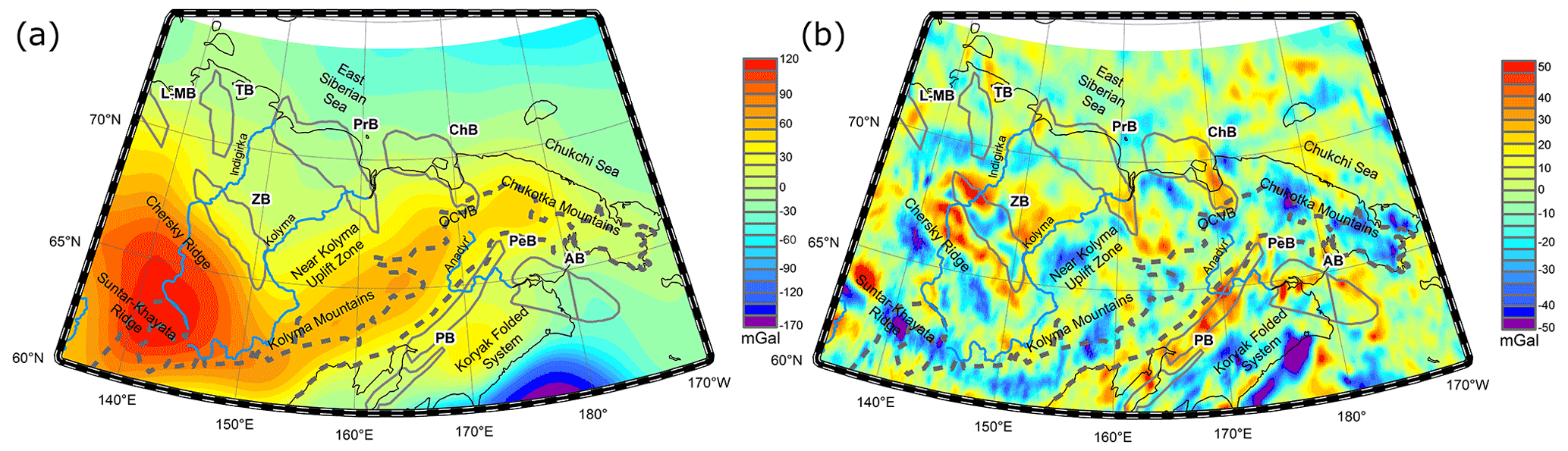
Figure 5 (a) Isostatic correction. (b) Residual isostatic gravity anomalies (also implying the effect of the initial model of sediments).

In the first adjusted model (Fig. 8a), several significant changes are visible, compared to the initial thickness of sediments (Fig. 2b). The second model (Fig. 8b) also displays some changes compared to the initial sedimentary thickness. The new model shows not only redistribution of the sedimentary thickness but also some changes that, as we suppose, refer to the structure of the crystalline crust, since we cannot completely divide these effects in the decompensative anomalies. Some of the new details on the sedimentary thickness distribution generally match the surface geology: however, some issues may raise questions, which are discussed in the next section.

6 Discussion

6.1 Sedimentary cover: model 1

The obtained models of the sedimentary cover generally repeat the large-scale features of the sedimentary thickness; however, some essential changes are visible. To display these details, we have prepared a set of the maps zooming in on some important regions. In Fig. 9, we provide a comparison between the initial sedimentary model (on the left) and two new models (the first model in the centre and the second one on the right).

In the model 1 (Fig. 8a), several areas of relatively large thickness (3–4 km) are found in the Chukotka Mountains area. They are likely related to thick volcanogenic deposits of relatively low density formed during the OCVB development. This zone continues as a 1–2 km deep conduit, bounding the continental Chauna Basin from the south. Then, this zone, with a characteristic thickness of 0.5–2 km, continues south-west and reaches the Sea of Okhotsk, repeating the OCVB shape and bounding its structures (e.g. the eastern slope of the Kolyma Mountains).

The thickness of many sedimentary basins has been significantly reduced in the new model compared to the initial one. Also, for some basins, the location of depo-centres has been changed. For example, the sedimentary thickness has been reduced in the Anadyr Basin (Fig. 9a, centre), especially in its continental part (to 1–2 km). Moreover, the deepest part of the continental Anadyr Basin is shifted south-east in the new model, still remaining within the continent, while the deepest part (the depo-centre) of the eastern segment, located within the sea shelf, remains in the same place as in the initial model. We refer the corresponding gravity effect of the sedimentary cover mainly to the Cenozoic sediments, less consolidated than the deeper Mesozoic strata. Antipov et al. (2008) demonstrate a regional map of the sedimentary thickness for the Anadyr Basin, which is also different from the initial one shown in Fig. 2b. Their model is based on several short (several tens of kilometres) common depth point (CDP) seismic profiles; no other seismic data are available for this structure. These profiles show high variability of the basement from 0.5–1 to 4 km at some local points, although the interpretation of reflectors is somewhat uncertain. The thickness of sediments is also reduced in the northern part of the basin like in our model. Although the thickness is higher in some very local depressions (Antipov et al., 2008), which are not resolved by the new model, the northward decrease trend is visible for the continental part in both models, indicating that the new modelling approach provides sufficiently reliable results, at least qualitatively.

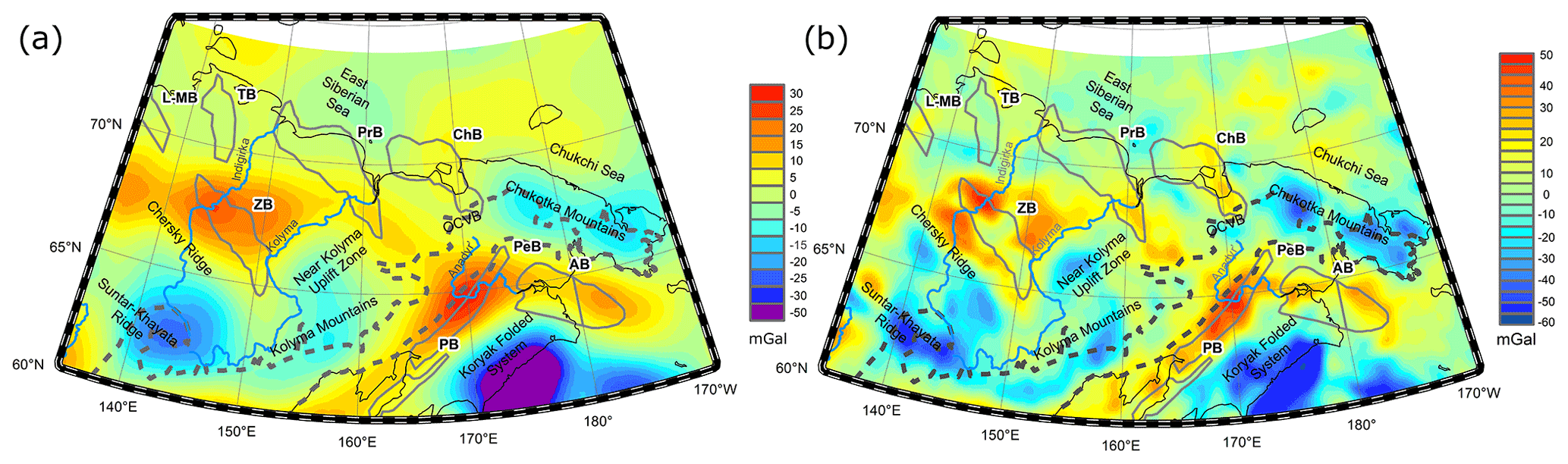
Figure 6 (a) Decompensative correction for the isostatic gravity anomalies. (b) Decompensative gravity anomalies.

In the new model, the thickness of the Penzhin Basin (Fig. 9b, centre) has also been reduced in the central part by about 2 times; however, it remains nearly the same near the borders. In contrast, the Pustorets Basin thickness is increased up to about 4 km compared to 2–3 km according to Clarke (1988), and the basin depo-centre is shifted to the south-east in the new model, being a part of the relatively deep zone continuing to the eastern coast of the Kamchatka Peninsula. However, the study of Clarke (1988) is an unpublished review not providing specific information about the data sources and especially of the methods.

Next, the new model displays a slight increase in thickness in the northern continental part of the Chauna Basin (Fig. 9c, centre) compared to the initial model (Fig. 9c, left). In the continental margin of the basin, the Cenozoic sedimentary thickness matches the drilling results (approximately 670 m including about 490 m of the Paleogene sediments, Aleksandrova, 2016). The sedimentary thickness in the offshore part of the basin referred to as the Ayon Basin (Fig. 9c) has been reduced to 2–2.5 km compared to the initial model, in which it reaches 4 km. Note that the new model agrees with the results of the seismic survey for the Ayon Basin, as seen in the map of Gresov and Yatsuk (2020), in which the Ayon thickness is also about 2.2–2.5 km. For the rest of the basin, the thickness distribution is nearly the same and increases from south-east to north-west.

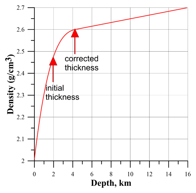
Figure 7 Illustration of the sedimentary thickness correction. This example corresponds to a negative decompensative anomaly.

We have found the most significant changes for the Zyryanka Basin (Fig. 9d). In the new model (Fig. 9d, centre), the basin is divided into three separate segments of approximately 2–2.5 km sedimentary thickness. Two of these separate segments correspond to the largest coal-bearing zones within the Zyryanka depression according to the map of Koporulin (1979) – the Myatis zone (north-western one) and the Zyryanka–Silyapsk zone (south-eastern one). Obviously, these zones, contoured with dashed lines in Fig. 9d, outline the Lower Cretaceous sedimentation. Like in the initial model, the south-eastern part of the Zyryanka Basin is deeper than the north-western one. Remarkable changes in the thickness have been found in the north-western segment. According to the new model, the 2–3 km thick north-western segment of the basin (the Myatis zone) is geometrically different from the one given in Koporulin (1979). It is divided into two branches at an almost right angle with respect to the main direction of this structure, and the newly revealed branch of slightly lower thickness is pointing north-east. As seen on the map from Koporulin (1979), another small zone of distribution of the Lower Cretaceous coal-bearing deposits, unidentified in the initial model, is located north-east from the Myatis zone (Fig. 9d), which again supports the new model. The last one shows a connection of these zones, although the shape of this north-eastern branch is not so clearly traced as compared to the segment related to the Zyryanka–Silyapsk zone. Although the map of Koporulin (1979) generally matches the shape of the new founded sedimentary thickness distribution, it was based on relatively old and geological studies and drilling data. It was mentioned by the author that the geological mapping and lithological-facies analysis of the basin strata, including the coal-bearing zones, was done by him and his predecessors in the 1960s–1970s with significantly different detail; therefore, some areas of the basin have been insufficiently studied. This gives reason to conclude that the lateral sedimentary thickness redistribution in the Zyryanka Basin is a new finding, showing the features of the Lower Cretaceous strata that were not previously mapped due to their overlap with the Cenozoic sediments and relatively sparse data.

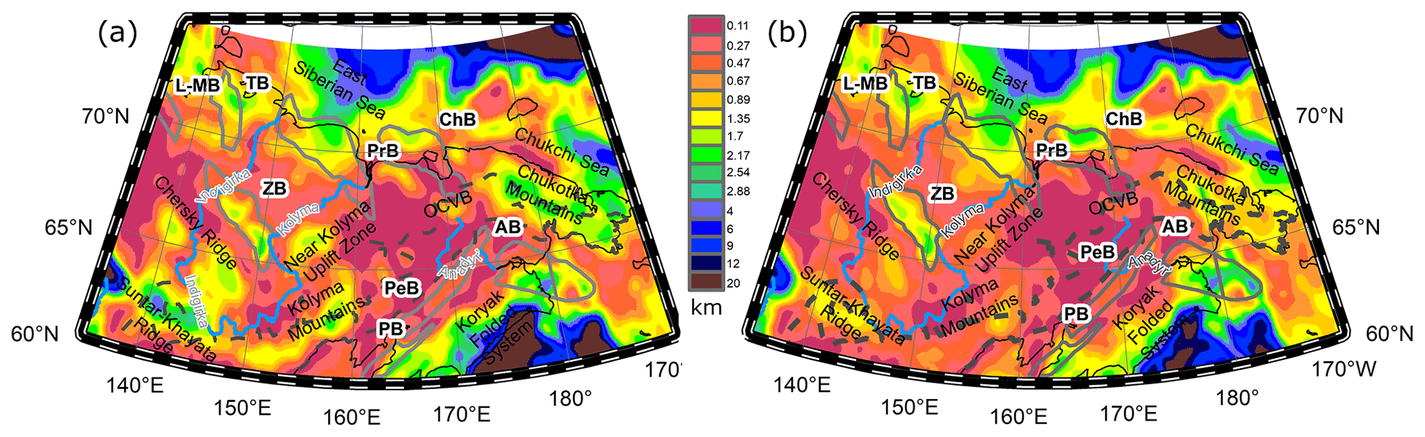
Figure 8 New model of sedimentary cover. (a) Model 1. (b) Model 2.

It should be noted that previous studies demonstrate significant differences and contradictions in mapping the sedimentary thickness for the Zyryanka Basin. Sitnikov et al. (2017) argue that the Lower Cretaceous sediments are up to 8 km thick in several parts of this depression, and that the Cenozoic sediments are more than 3 km thick. Similar conclusions for the maximal sedimentary thickness of 7–9 km were made earlier by Koporulin (1979). Stoupakova et al. (2017) even mention 8–10 km of total thickness. However, neither the initial sedimentary model used in this study nor the sedimentary map for the Arctic (Petrov et al., 2016) indicates such thickness of sediments in the Zyryanka Basin. Actually, most of the old maps are based on very sparse, unsystematic, and obsolete results based on outdated methods, e.g. interpretation of the Bouguer gravity anomalies or magnetic data. Our study shows that the sedimentary thickness should be about 3 km lower in the deepest parts.

The Primorsk Basin (Fig. 9e) is also poorly studied by seismic surveys (Pavlova, 2020), which revealed only the basic features of the sedimentary structure for shallow depths often not reaching the basement. According to these seismic data, the uppermost layers are represented by Neogene–Quaternary sediments (including alluvial) up to 1.2 km thick and the underlying Mesozoic to Cenozoic sediments up to 2 km thick. It is clear that the new model (Fig. 9e, centre) generally agrees both with the initial one (Fig. 2b) and with the results obtained from the sparse seismic studies, and the sedimentary thickness of the Primorsk Basin remains almost the same as in the initial model for its deepest part (2–2.2 km). However, the thickness of the Primorsk Basin is significantly reduced in its south-eastern part. This lateral variability of the sedimentary thickness is discovered for the first time in the present study.

The maximal sedimentary thickness of the Tastakh Basin (Fig. 9e) is about 2.5–3 km in its depo-centre according to the new model. From the comparison of the initial model (Fig. 9e, left) and the new one (Fig.9e, centre), no significant changes in the sedimentary thickness appeared after the decompensation correction, and the basin shape remains the same. Sitnikov (2017) and Sitnikov and Sleptsova (2020) also pinpointed the sedimentary thickness values from 1.5 to 3 km for the basin. The Lower Jurassic rocks at the bottom of the CDP transect presented in Sitnikov (2017) can be regarded as a relatively dense transition layer between the basement and the sedimentary cover, which gives only a little effect in the gravity field; and this is the reason why the new sedimentary model does not show depths of more than 3 km for this basin. The segment of the Laptev–Moma system in the studied area, including the rifts filled with Cenozoic sediments, was not changed significantly.

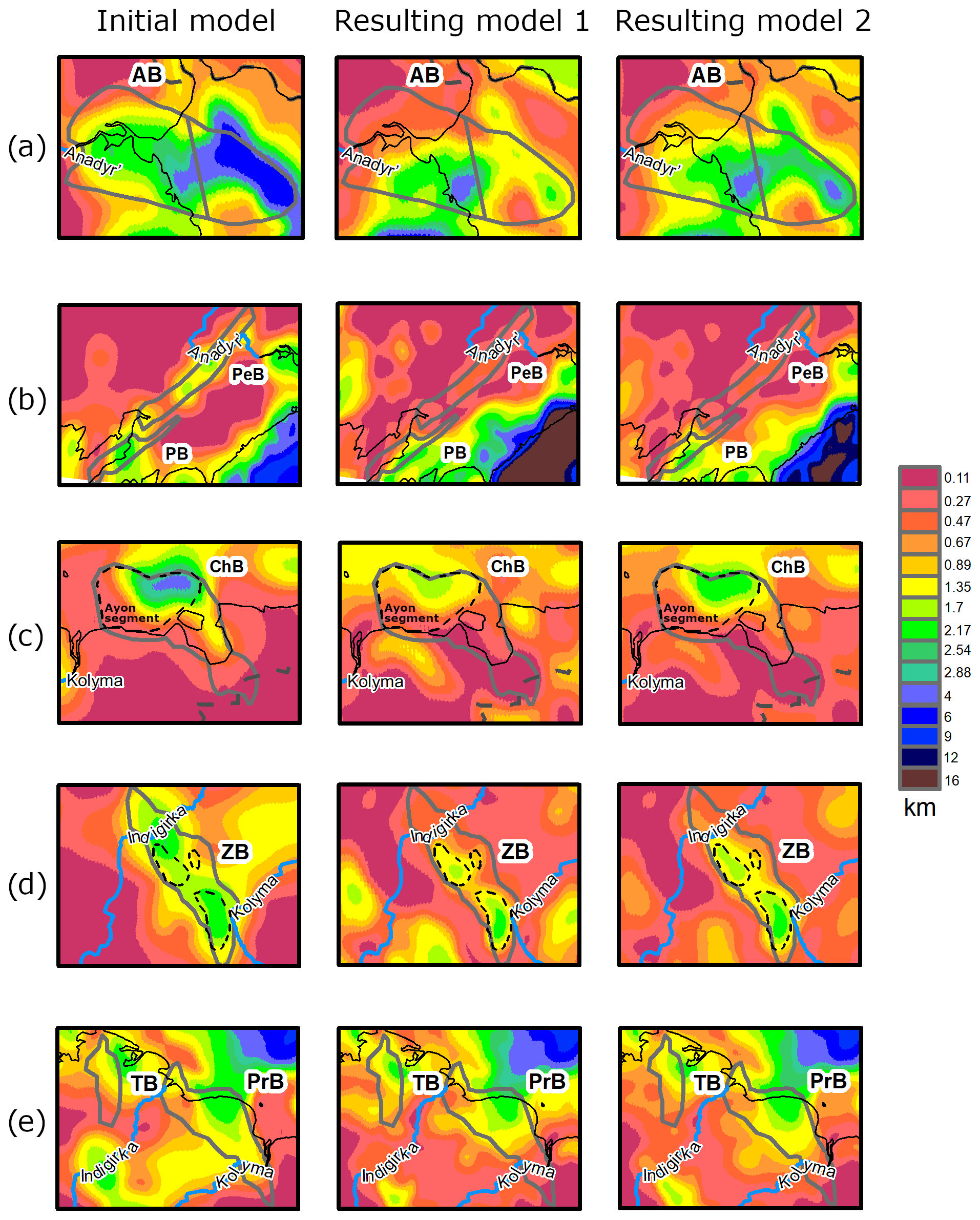
Figure 9 Comparison between the initial sedimentary model (left) and the new sedimentary cover models – 1 (centre) and 2 (right) – for several basins: Anadyr (a), Penzhin and Pustorets (b), Chauna (c), Zyryanka (d, dashed lines show the Lower Cretaceous coal-bearing zones), Primorsk and Tastakh (e).

Potential uncertainties of the obtained model increase with depth since the difference in density with the crystalline rocks is insignificant for deep layers and even relatively thick sediments produce only a small effect in this case. Therefore, even an insignificant negative decompensative anomaly could lead to a noticeable increase in the basement's depth if it was initially deep (Fig. 7). For example, the density of Late Cretaceous sediments in the region might be quite large, especially in the intermontane depressions, due to the Late Mesozoic and even Cenozoic metamorphism. In the eastern part, the basins bounding the OCVB could include the Cretaceous layer as a transition between the folded basement and less dense upper layers. This factor could also lead to significant differences with seismic models, which interpret relatively high seismic wave velocities in the lower (ancient) part of the sedimentary cover as the basement (e.g. for shallow Lower Cretaceous deposits in the Verkhoyansk region). So, for the deep basins, the model should be considered qualitative rather than quantitative. Finally, an additional gravity effect can be associated not only with sedimentary layers but also with the upper part of the crystalline crust, resulting in an artificial increase in the sedimentary thickness in the final model.

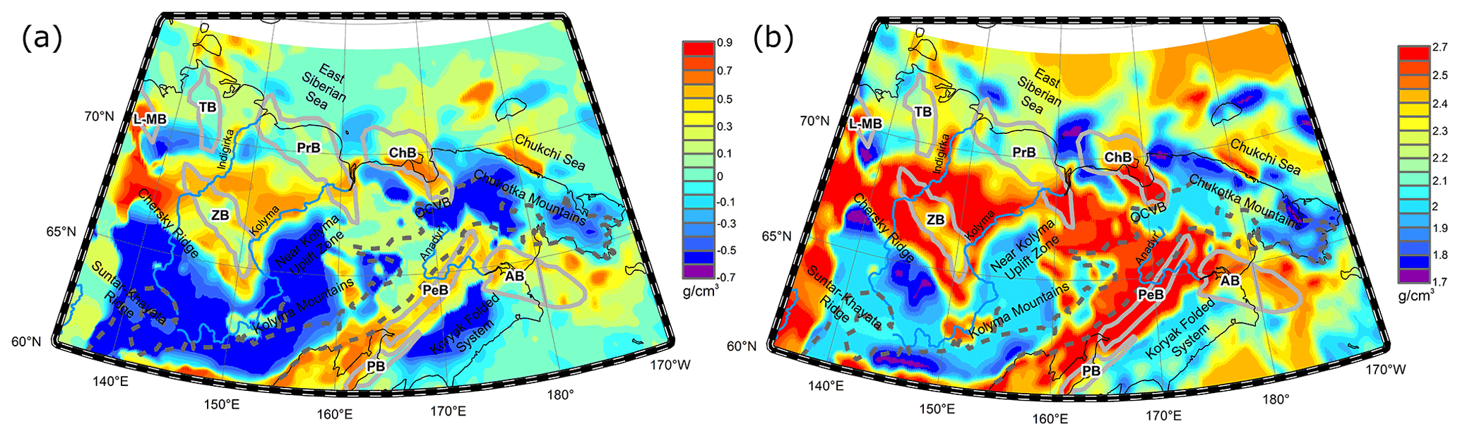
Figure 10 (a) Density correction. (b) Corrected density model (vertically averaged).

Potential uncertainties of the sedimentary thickness determined from the decompensative gravity anomalies were assessed by Kaban et al. (2021a). They assume that the uncertainty of the density–depth relation is approximately 15 % (Mooney and Kaban, 2010). Then, for the thickness of 2 km, actual values would be in the interval 1.55–2.6 km; and for the thickness of 4 km, they are within 2.9–5.35 km. For deep basins (approximately > 7.5 km), the upper limit is indefinite. Therefore, for depths larger than 7 km, the thickness estimations are rather qualitative.

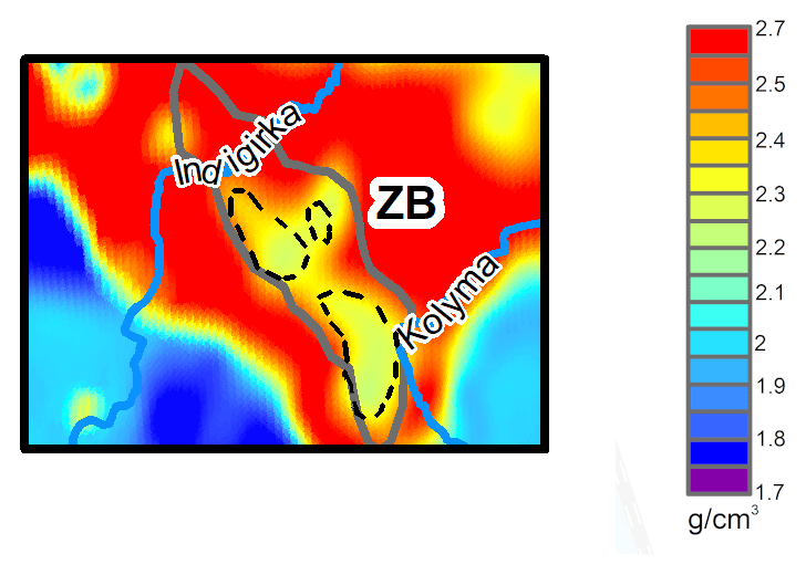
Figure 11 New density model zoomed in on the Zyryanka Basin. Dashed lines show the Lower Cretaceous coal-bearing zones.

6.2 Sedimentary cover: model 2

In the second model (Fig. 8b), we assumed that half of the decompensative anomaly is related to the changes in the sedimentary thickness and the other half to the density of sediments. Despite some changes in the thickness, qualitatively, its distribution remained similar to the first model.

In the second model, the OCVB zone is within 1.2–2 km and traced to the same position as in the first model. However, due to the different initial conditions, this zone is smoother and has fewer small-scale details, although they generally repeat the OCVB shape. The main depression zone is now wider. Like in the first model, the thickness of sediments is reduced in the Zyryanka Basin and, in general, in the Primorsk and Tastakh basins, but, at the same time, their outlines remain almost the same as in the first model. The thickness of the offshore part of the Chauna Basin (its Ayon segment) has been decreased 2 times compared to the initial model (Fig. 9c).

Some significant differences in thickness and shape are found for the Anadyr Basin (Fig. 9a, right). The maximal thickness in the second model is shifted to the south-east less than in the first model, but in both cases its position differs from the one in the initial model. At the same time, the position of the depo-centre of the offshore part is basically the same in all three models. Possible reasons for the migration of the continental thickness maximum of the Anadyr Basin in both corrected models might be related to the heterogeneous structure of its folded basement and of the deep sedimentary layers (Clarke, 1988). The northern and north-western parts of the basement mainly consist of the Late Cretaceous OCVB rocks (effusives, tuffs, etc.), while its south-eastern part formed in the conditions of the Okhotsk–Chukotka active continental margin from the end of the Early Cretaceous to the beginning of the Late Cretaceous, when the adjacent Koryak (Anadyr–Koryak) folded system formed as an accretionary prism of the subduction zone. The lower layers of the sedimentary cover are presented in the south and south-west, close to the Koryak folded system, and are of the Albian–Cenomanian, later Upper Cretaceous, and early Paleocene age. These strata are often regarded as a transition layer between the basement and sediments (Antipov et al., 2008). Moreover, the Cenozoic section, contributing to the main 2–3 km part of the cover, is distributed more widely than the above-mentioned transition complex, with thickness decreasing from south to north. Application of the decompensative corrections reveals these lateral sedimentation irregularities and leads to the changes in the thickness in both resulting models.

The thickness variations in the Pustorets Basin in the second model (Fig. 9b, right) are close to the initial model (Fig. 9b, left), while the absolute thickness is generally lower than in the first model, with smoother variations. The depo-centre position is similar to the first model (Fig. 9b, left). The Penzhin Basin location was not changed, although the sedimentary thickness is reduced (Fig. 9b, right). Finally, the sedimentary structure of the Laptev–Moma system (Shiroston and Ust'–Yana rifts) in the second model remains nearly the same as in the first model. The reason for this is the relatively insignificant depth of the sedimentary strata filling the rifts: it is about 1–2 km, as mentioned in Drachev et al. (2010) and Drachev (2016), and it is reduced to 1 km or even less on the basement height between the Shiroston and Ust'–Yana grabens. The density of the sediments filling the rift is relatively high.

The corrections for the initial density of sediments (Fig. 10a) are within the range of −0.7 to 0.9 g/cm³. The obtained sedimentary density model (Fig. 10b), in our opinion, should be interpreted qualitatively rather than quantitatively as the density of sediments is vertically averaged and potentially anomalous layers are not identified. The calculated density distribution generally matches the new features of the sedimentary thickness after the decompensative correction. For example, the 2.2–2.4 g/cm³ zone corresponding to the Zyryanka Basin (Fig. 11) repeats the shape of the new thickness map based on the decompensative gravity anomalies. The results show a clear relation between the north-western zone of the Lower Cretaceous coal-bearing molasses and the larger Myatis zone (the corresponding zones are contoured by dashed lines in Fig. 11). It is visible in the map (Fig. 10b) that the average density of sediments increases with thickness due to compaction under the increased pressure. Large density changes are also related to the mountain areas of the Verkhoyansk orogeny (e.g. the Chersky Ridge) and the OCVB structures in its northern segment. The difference between the density of these structures and the density of thick sediments is moderate.

The new sedimentary models were calculated based on the assumption that the decompensative anomalies are exclusively induced by changes in the sedimentary basins' structure (thickness in the first model and both thickness and density in the second one) by applying the approach of Kaban et al. (2021b). Another possible source of the decompensative anomalies, especially in the case of positive ones, could be local densification of the upper crust due to intrusive rocks or metamorphism, the effects of which were not considered in this study. Therefore, the resulting models may include possible local uncertainties in the vicinity of the intrusions related to the OCVB structure. However, for most of the sedimentary basins in the study area, these uncertainties are generally local and, therefore, minor with respect to the large-scale structures.

7 Conclusions

This study presents the new sedimentary cover models for the eastern Asia Arctic zone based on the analysis of the decompensative gravity anomalies. First, we computed the isostatic gravity anomalies for the study area, and then we applied the decompensative correction to the isostatic anomalies. The correction spans the range of −50 to +30 mGal and principally changes the isostatic anomaly patterns. Two sedimentary cover models, differing in their initial conditions, have been obtained from the decompensative anomalies. The main discoveries are as follows:

• Essential changes in the sedimentary thickness and the depo-centre location have been found for the Anadyr Basin in its continental part, where the thickness has been reduced to 1–2 km.

• New details of the sedimentary thickness variations have been revealed for the central part of the Penzhin Basin, where the thickness appeared to be lower by about 2 times compared to the initial model, and for the Pustorets Basin, for which the new location of the depo-centre has been identified.

• For the offshore part of the Chauna Basin (referred as the Ayon Basin), the sedimentary thickness appears to be 2–2.5 km in the new model, which is lower than in the initial model (4 km). The new result agrees with the marine seismic surveys, which confirms robustness of the method.

• The most significant lateral redistribution of the sedimentary thickness has been found for Lower Cretaceous coal-bearing strata in the northern part of the Zyryanka Basin. The new model indicates the connection of two coal-bearing zones, revealing the features of the Lower Cretaceous strata that were not previously mapped due to insufficient geological surveys.

• New details on the sedimentary thickness variations have been discovered for the Primorsk Basin. The sedimentary thickness in the basin is significantly reduced in the south-east direction.

As we mentioned before, it is impossible to completely separate the effects of the sedimentary cover density anomalies from those ones in the upper crust. Therefore, the new models may display some artificial features, which appear due to neglecting the crystalline crust density heterogeneity. Nevertheless, the overall analysis of two new models confirms the efficiency of the approach based on the decompensative gravity anomalies. This approach application has made it possible to reveal several essential changes in the geological structure of the analysed sedimentary basins. In many cases, the results of our study are the only ones providing the information on the structure of sedimentary basins.

In the interpretation of the obtained models, some issues remain unexplained. For example, the rocks of similar age forming the basins are sometimes considered here in different ways because the tectonic development of the study area was different and its relatively younger segments were formed in its eastern part. For the Anadyr, Penzhin, and Pustorets basins, the Cretaceous rocks form the folded basement, while most of the eastern part of the study area is covered by the volcanic rocks (of the late Early Cretaceous–Late Cretaceous age and younger), resulting in reduced sedimentary cover in both new models.

Previous geophysical studies in the region under consideration are very sparse and represented by old and unsystematic results. Furthermore, the employed indirect geophysical methods (gravity, magnetic) are outdated, while direct seismic data are available only for limited locations. Thus, despite detailed surface geology surveys, the sedimentary thickness is still poorly mapped in the whole region. The present study provides for the first time a consistent map for the whole Arctic zone of north-eastern Asia based on unified standards of interpretation. It confirms that this method can be used for investigations of hardly accessible areas as was previously done for Antarctica (Haeger and Kaban, 2019) and for the Congo Basin (Kaban et al., 2021a). Finally, the obtained results can be used for the future planning of detailed studies of local structures within the study region, which have the potential for mineral prospecting and exploitation and for the infrastructure development important for the Arctic zone.