Seismicity during and after stimulation of a 6.1 km deep enhanced geothermal system in Helsinki, Finland

In this study, we present a high-resolution dataset of seismicity framing the stimulation campaign of a 6.1 km deep enhanced geothermal system (EGS) in the Helsinki suburban area and discuss the complexity of fracture network development. Within the St1 Deep Heat project, 18 160 m³ of water was injected over 49 d in summer 2018. The seismicity was monitored by a seismic network of near-surface borehole sensors framing the EGS site in combination with a multi-level geophone array located at ≥ 2 km of depth. We expand the original catalog of Kwiatek et al. (2019), including detected seismic events and earthquakes that occurred 2 months after the end of injection, totaling 61 163 events. We relocated events of the catalog with moment magnitudes between M_w −0.5 and M_w 1.9 using the double-difference technique and a new velocity model derived from a post-stimulation vertical seismic profiling (VSP) campaign. The analysis of the fault network development at a reservoir depth of 4.5–7 km is one primary focus of this study. To achieve this, we investigate 191 focal mechanisms of the induced seismicity using a cross-correlation-based technique. Our results indicate that seismicity occurred in three spatially separated clusters centered around the injection well. We observe a spatiotemporal migration of the seismicity during the stimulation starting from the injection well in the northwest–southeast (NW–SE) direction and in the northeast (NE) direction towards greater depth. The spatial evolution of the cumulative seismic moment, the distribution of events with M_w≥1, and the fault plane orientations of focal mechanisms indicate an active network of at least three NW–SE- to NNW–SSE-oriented permeable zones, which is interpreted to be responsible for the migration of seismic activity away from the injection well. Fault plane solutions of the best-constrained focal mechanisms and results for the local stress field orientation indicate a reverse faulting regime and suggest that seismic slip occurred on a sub-parallel network of pre-existing weak fractures favorably oriented with the stress field, striking NNW–SEE with a dip of 45^∘ ENE parallel to the injection well.

1 Introduction

Deep geothermal energy is considered a potential source of low-CO₂-emission energy to replace fossil fuels. The successful development of deep geothermal reservoirs is crucial for the economic production of hot fluids for energy generation. However, crystalline basement rocks hosting deep geothermal reservoirs in general are low-porosity and low-permeability formations. In enhanced geothermal systems (EGSs) hydraulic stimulation with massive fluid injection is applied to improve reservoir permeability (e.g., Giardini, 2009). Fluid injection at depth in EGS stimulations and in wastewater disposal is commonly associated with induced seismicity (e.g., Ellsworth, 2013; Majer et al., 2012). Successful mitigation of an induced seismic hazard is important for public acceptance of geothermal projects, as there is significant concern related to the occurrence of larger induced earthquakes during previous EGS projects, e.g., in Basel and St. Gallen, Switzerland (e.g., Giardini, 2009; Diehl et al., 2017), and most recently in Pohang, South Korea (Hofmann et al., 2019; Ellsworth et al., 2019).

A well-designed seismic network is a prerequisite for high-resolution data acquisition, real-time seismic monitoring, and analysis of induced seismicity (e.g., Bohnhoff et al., 2018). Subsequent feeding of seismic data into a traffic-light system (TLS) may substantially contribute to mitigating the associated seismic hazard and risk. A successful and safe approach to stimulation of the world's deepest EGS in the metropolitan area of Helsinki was recently presented by Kwiatek et al. (2019). Over 49 d in summer 2018, the St1 Deep Heat Company injected more than 18 000 m³ of water at 6.1 km of depth. An M 2.1 red alert threshold of the TLS defined by the local authorities was successfully avoided by a careful adjustment of the hydraulic energy input in response to real-time monitoring of the spatiotemporal evolution of seismicity. The largest seismic event was confined to a moment magnitude of M_w 1.9 (Ader et al., 2019; Kwiatek et al., 2019).

High-quality state-of-the art analysis of induced seismic waveform data is crucial for a detailed reservoir characterization (Kwiatek et al., 2013). High-precision locations of hypocenters are typically obtained by applying relocation techniques such as the double-difference method (Waldhauser and Ellsworth, 2000). Using relocated data, a precise spatiotemporal evolution of induced seismicity can be tracked, providing insight into fluid migration pathways in the reservoir (e.g., Kwiatek et al., 2015; Diehl et al., 2017). In addition, seismic source parameters such as seismic moment and source size provide crucial insights into the fracture network geometry.

Bentz et al. (2020) recently showed that many EGS fluid injections display an extended period of stable evolution of the cumulative seismic moment. Following Galis et al. (2015), this indicates the growth of self-arrested ruptures in contrast to unstable increases in seismic moments resulting in runaway ruptures that are only limited by the size of tectonic faults. Thus, unusual trends or potential changes in the seismic moment evolution may provide information on growth and activation of ruptures and thus also on the anthropogenic seismic hazard and subsequent risk. For example, Bentz et al. (2020) observed a steep and non-stabilizing increase in the cumulative seismic moment, potentially signifying unbound rupture propagation during stimulation for the Pohang EGS project. Dynamic source characteristics of seismic events including radiated energy, stress drop, and apparent stress allow the evaluation of seismic injection efficiency (Maxwell et al., 2008) and the estimation of the energy budget of a stimulation campaign. Moreover, focal mechanisms provide important information for hazard assessment, as they can illuminate activation of large pre-existing structures such as major and potentially critically pre-stressed faults (e.g., Deichmann and Giardini, 2009; Ellsworth et al., 2019). Using focal mechanisms, Ellsworth et al. (2019) showed that induced seismicity activated a fault zone, which ultimately triggered the large M_w 5.5 earthquake in Pohang. The authors suggested that seismic analysis performed during stimulation sequences may provide early information on increasing seismic hazard. In addition, stress tensor inversion of focal mechanism data using, e.g., the MSATSI (Martínez-Garzón et al., 2014) or BRTM (D'Auria and Massa, 2015) approaches allows the estimation of potential changes in the local stress field but requires high-quality seismic waveform data from dense local seismic networks. Studies of the spatial and temporal variations of the stress field orientation contribute to understanding complex seismo-mechanical processes occurring in the reservoir during injection (Kwiatek et al., 2013). Martínez-Garzón et al. (2013) first observed a clear correlation of temporal stress changes in response to high injection rates at The Geysers geothermal field.

In this study we present a refined high-resolution dataset of seismicity induced during stimulation of the world's deepest EGS in the Helsinki suburban area in 2018 (Kwiatek et al., 2019; Ader et al., 2019; Hillers et al., 2020). The data were collected using a combined seismic network of individual sensors in shallow boreholes framing the injection site combined with a multi-level vertical geophone array at ≥ 2 km of depth. Our dataset expands, refines, and completes the original study of Kwiatek et al. (2019). We include seismic events that occurred after the end of the hydraulic stimulation and refine the seismic catalog using double-difference relocation with a new velocity model derived from a post-injection vertical seismic profiling (VSP) campaign. To analyze the structural complexity of the reservoir, we investigate the spatiotemporal seismicity evolution as well as the temporal and spatial distribution of the seismic moment release during and after stimulation. This analysis is supported by an extensive catalog of source mechanisms derived from a cross-correlation-based technique. Information on the local stress field orientation is derived from seismicity data. We discuss the evolution of potentially permeable zones in the reservoir and the reactivation of a network of small-scale fractures during and after stimulation.

2 Methodology

Expanding the study of Kwiatek et al. (2019), we enhanced, reprocessed, and relocated the original seismic catalog to also include post-injection events between 22 July and 24 September. During and after the stimulation, induced seismicity was monitored by a dense seismic network of three-component sensors consisting of a 12-level vertical borehole array and 12 near-surface seismometers with full azimuthal coverage. The borehole array with 15 Hz sensors, sampled at 2 kHz, was installed at a depth from 1.95 to 2.37 km in the monitoring well OTN-2 close to the injection well OTN-3, whereas the 4.5 kHz near-surface seismometers, sampled at 500 Hz, were placed in wells with depths from 0.3 to 1.15 km and lateral distances of 0.6 to 8.2 km around the injection well (Fig. 1).

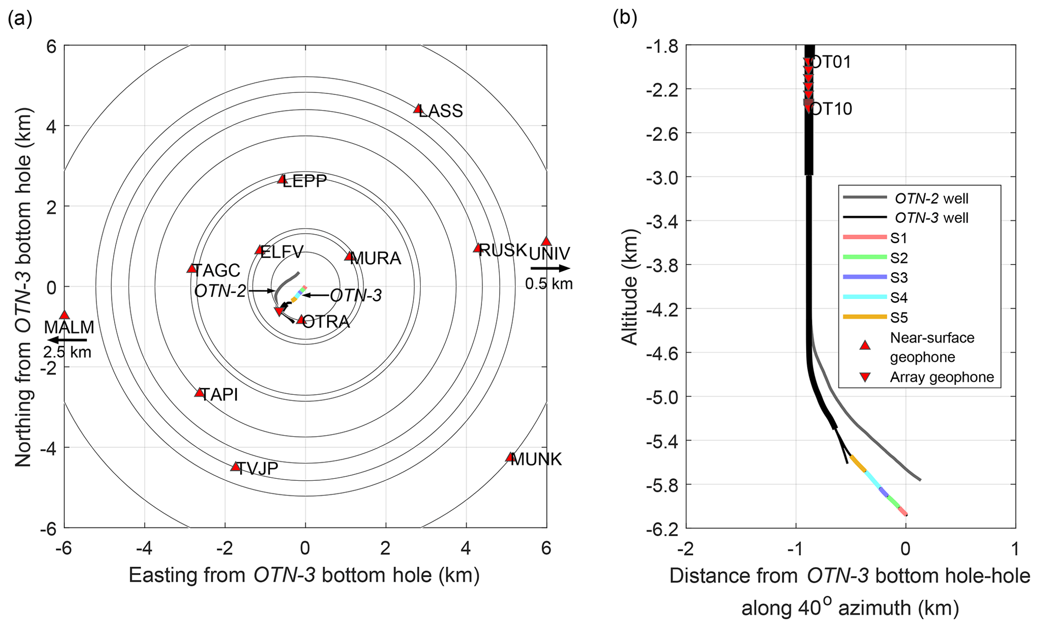
Figure 1 Seismic network used for monitoring the stimulation in 2018. (a) Map view showing the near-surface geophones framing the EGS site with the injection borehole OTN-3 and the OTN-2 well drilled in 2019 and 2020. The radius of concentric circles represents the distance between the end of the OTN-3 borehole and each station. (b) Side view of the boreholes with the geophone array placed at the already existing part of the OTN-2 well. The injection intervals S1–S5 of the stimulation in 2018 are color-coded at the end of the injection borehole. For further details about the location of the EGS site in the suburban area of Helsinki in Finland, see Kwiatek et al. (2019).

The reprocessed seismic catalog, with a description of its properties, is available as a separate data publication (Leonhardt et al., 2021) and consists of 5456 events with $M_{\mathrm{w}}\ge -\mathrm{2.47}$ that were detected and located during and after the stimulation (industrial monitoring) and reprocessed in our study. A total of 55 707 events with $M_{\mathrm{w}}\ge -\mathrm{0.9}$5 were further detected during and after the stimulation but were not located or processed later on. These were also included in the published seismic catalog. For a further explanation of the original seismic catalog, see Kwiatek et al. (2019).

2.1 Hypocenter locations

The enhanced sub-catalog of 5456 events including 946 post-stimulation events was reprocessed by applying a new updated 1D layered velocity model developed from P-wave onset times of calibration shots obtained during a post-injection VSP campaign (Fig. S1; see also Leonhardt et al., 2021). Due to a low signal-to-noise ($S/N$) ratio of the VSP data, the S-wave arrival times could not be determined. Thus, the $V_P/V_S$ ratio was optimized by a trial-and-error procedure, whereby we ultimately constrained a $V_P/V_S$ ratio of 1.71 that minimized the cumulative residual errors of all located events and at the same time kept the first induced events close to corresponding injection well OTN-3.

The hypocenter locations were estimated using the equal differential time (EDT) method (Zhou, 1994; Font et al., 2004; Lomax, 2005) and the new VSP-derived velocity model. In addition, station corrections were applied. The minimization of travel time residuals,

$$\begin{array}{}\text{(1)}& {\left|\left|\left(T_j^{\mathrm{th}}-T_i^{\mathrm{th}}\right)-\left(T_j^{\mathrm{obs}}-T_i^{\mathrm{obs}}\right)\right|\right|}_{L_{\mathrm{2}}}=\min ,\end{array}$$

where T^th and T^obs are all unique pairs (i,j) of theoretical and observed travel times of P- and S-phases, was resolved using the Simplex algorithm (Nelder and Mead, 1965; Lagarias et al., 1998) . A total of 2958 reprocessed events were located around the injection well OTN-3 at an epicentral distance of less than 5 km and at a depth of 4.5 to 7 km. The hypocenters of these events were included in the reprocessed and published data catalog.

To further refine the quality of hypocenter locations, 2178 of the 2958 absolute located events with at least 10 P-wave and 4 S-wave picks were selected, and the double-difference relocation technique (hypoDD) was applied using the new VSP-derived velocity model (Waldhauser and Ellsworth, 2000). An iterative least-square inversion was used to minimize residuals of observed and predicted travel time differences for event pairs calculated from the existing P- and S-wave picks of the selected catalog data. The residuals were minimized in 10 iterations steps. For the last iteration, the maximum threshold for travel time residuals was set to 0.08 s, and the maximum distance between the catalog linked event pairs was defined as 170 m. With the hypoDD method 1986 events were relocated, representing 91 % of the selected 2178 events. The residuals of the relocations have a root mean square error of 9 ms. The relocation uncertainties were then assessed using a bootstrap technique (Waldhauser and Ellsworth, 2000; Efron, 1982), leading to a relative location precision not exceeding ± 52 m for 95 % of the catalog.

2.2 Source mechanisms

To address the structural complexity of the reservoir in close proximity to the injection borehole below 4.5 km of depth, source mechanisms were determined for a selected subset of events. For the 63 events with the largest moment magnitudes located within the main (deepest) hypocenter cluster we first manually picked the P-wave onset polarities on the vertical component seismograms of all available stations. All waveforms were first filtered with a second-order 120 Hz low-pass Butterworth filter. The same approach was applied to the 25 strongest events of the two shallower hypocenter clusters (see Fig. 3). The focal mechanisms (FMs) were determined using the HASH software (Hardebeck and Shearer, 2002). For each fault plane solution (FPS), associated uncertainties in a form of acceptable solutions are provided, calculated by perturbing take-off angles and azimuths by up to 3^∘ (95 % confidence interval) to simulate the hypocenter location and velocity model uncertainties, respectively.

Aiming to increase the catalog of focal mechanisms, we extended the focal mechanism calculations to smaller events with lower $S/N$ ratios using the cross-correlation-based technique of Shelly et al. (2016). An additional 297 small events with a lower $S/N$ ratio were processed. To this end, the waveforms from a template set of 70 events with manually picked P-wave polarities were used to recover relative polarities of a target set of waveforms from 297 events, including 45 post-stimulation events and 18 events with manually picked polarities. The waveforms of the events of both sets were first preprocessed by focusing on the P-wave polarities obtained from the vertical components of all available stations. Seismograms were filtered with a second-order 120 Hz low-pass Butterworth filter and a window length of 0.064 s, including 0.012 s before the P-wave first motion. After a few trials, the low-pass Butterworth filter was fixed to 80 Hz for three stations in the satellite network due to a higher quality of the estimated polarity results for these stations. Considering the stations separately, each extracted waveform from the target set was cross-correlated with all remaining waveforms forming the template set. This resulted, for a particular station and target event, in a vector of 70 cross-correlation (CC) coefficients, with the sign representing the relative polarities between the target and template P-wave onsets for a particular station. Following Shelly et al. (2016), if the lag time of the largest cross-correlation peak was lower than 0.2 times the extracted wavelength, the CC was accepted and used as a relative polarity estimation between target event and template. The polarity estimates obtained from the CC values between the picked template and target events are relative and weighted by the absolute value of the corresponding cross-correlation coefficient. Thus, the sign of the estimated polarity of the target event will be positive if the template and the target event have the same P-wave first motion.

For each station k, the vectors containing relative polarity estimates between one target event i and all templates j were gathered in a i-by-j matrix. A singular value decomposition (SVD) was applied to the relative estimated polarity matrix of each station k to extract the strongest common signal of any target event obtained by the first left singular vector of the SVD (Shelly et al., 2016; Rubinstein and Ellsworth, 2010). The estimated first left singular vectors for each station k are gathered in an i-by-k matrix:

$$\begin{array}{}\text{(2)}& {\mathbf{PP}}_{ik}=\left[\begin{array}{ccc}p{p}_{\mathrm{11}}& \mathrm{\cdots }& p{p}_{\mathrm{1}k}\\ \mathrm{⋮}& \mathrm{\cdots }& \mathrm{⋮}\\ p{p}_{i\mathrm{1}}& \mathrm{\cdots }& p{p}_{ik}\end{array}\right],\end{array}$$

which then represents the most reasonable but still relative polarity pattern of each target event.

To reduce the polarity ambiguity of the events, we considered 18 events with known manually picked polarities included in the target event set. For each station k, the SVD-derived polarities of these events were compared with manually picked polarities to investigate whether the polarities have similar or opposite signs. In the case of the same polarities, the SVD-derived polarities of other events should also show the right sign for the particular stations.

Estimated polarity patterns of the events were then used to calculate focal mechanisms. For further investigation we only considered events with a good quality of estimated focal mechanisms no matter if the polarities were manually picked or estimated. Thus, we only used events with focal mechanisms that have root mean square fault plane uncertainties less than or equal to 35^∘ (Hardebeck and Shearer, 2002). The final catalog of focal mechanisms includes 191 events with either a manual or estimated polarity pattern and is presented with associated uncertainties in the data publication (see Leonhardt et al., 2021).

2.3 Complexity of source mechanisms

To investigate the variability of the estimated focal mechanisms, we first calculated the principal axis directions of the double-couple seismic moment tensor derived from the focal mechanism for each event. To quantify the level of similarity of any two focal mechanisms, we calculated the 3D Kagan rotation angle between the principal axis directions of both events (Kagan, 1991, 2007; Tape and Tape, 2012). Low values of the Kagan angle (<20^∘) suggest that focal mechanisms of two events are similar. To further group events into families with similar source mechanisms, an unsupervised classification of the 191 events was performed using a hierarchical cluster analysis based on the similarity of estimated Kagan rotation angles. Thus, the measurement of proximity PR of any two focal mechanisms was defined as a distance metric:

$$\begin{array}{}\text{(3)}& {\mathbf{PR}}_{ij}={\displaystyle \frac{\mathrm{1}-\cos \left({\mathit{\theta }}_{ij}^{\mathrm{rot}}\right)}{\mathrm{1.5}}},\end{array}$$

where ${\mathit{\theta }}_{ij}^{\mathrm{rot}}$ is a matrix containing the estimated rotation angles between any focal mechanism pair ij. In the following, the dendrogram tree based on the hierarchical clustering was used to separate focal mechanisms into different families.

To investigate the local stress field orientation in the reservoir surrounding the injection well, we applied the linear stress inversion method MSATSI (Martínez-Garzón et al., 2014) and the Bayesian-analysis-based and nonlinear stress inversion method BRTM of D'Auria and Massa (2015). In both methods, the strike, dip, and rake angles of the fault plane solutions from the focal mechanisms were used to invert the orientation of three stress axes. A relative measure of the stress magnitude is obtained by the stress shape ratio R (e.g., Hardebeck and Michael, 2006; Lund and Townend, 2007):

$$\begin{array}{}\text{(4)}& R={\displaystyle \frac{{\mathit{\sigma }}_{\mathrm{1}}-{\mathit{\sigma }}_{\mathrm{2}}}{{\mathit{\sigma }}_{\mathrm{1}}-{\mathit{\sigma }}_{\mathrm{3}}}}.\end{array}$$

3 Results

3.1 Seismic catalog update

The moment magnitudes of the absolute located and relocated seismicity are plotted with time during and after shut-in as grey and orange dots in Fig. 2. The five different stimulation phases (P1–P5) performed in 2018 are also shown in Fig. 2 in combination with the wellhead pressure and seismic event rate. Further details of the stimulation protocol and seismicity evolution are presented by Kwiatek et al. (2019), and here we focus on analysis of post-stimulation seismicity.

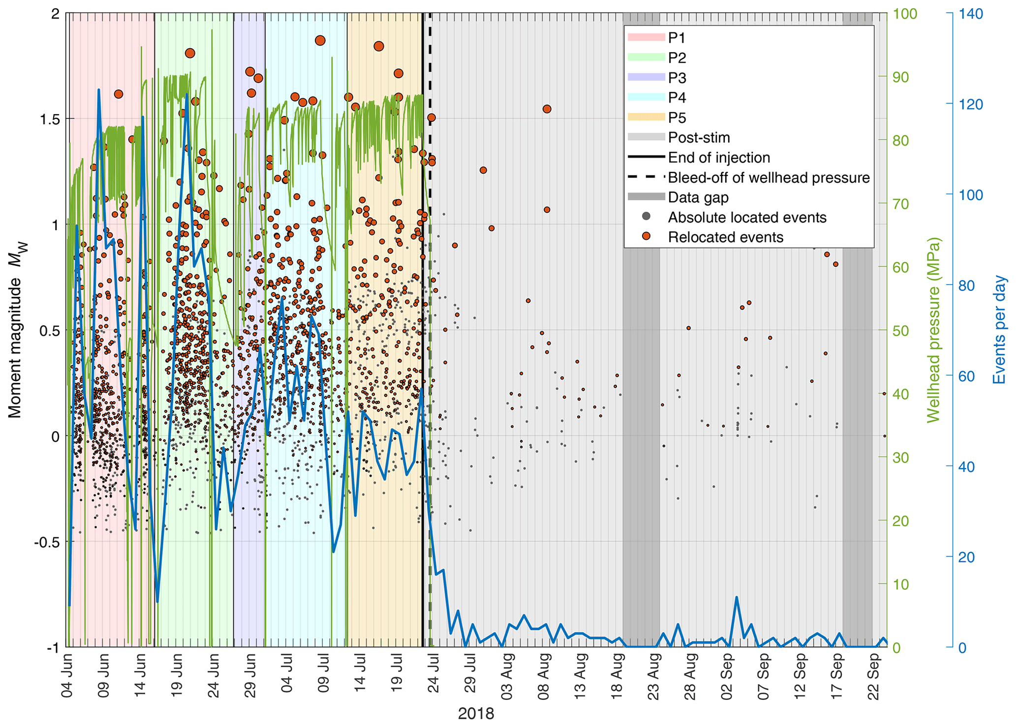
Figure 2 Stimulation protocol with moment magnitudes of induced seismicity during stimulation phases P1–P5 and post-stimulation time period. The magnitudes of 2958 absolute located and 1986 relocated events are shown as grey and orange dots, respectively. The solid green line represents the wellhead pressure during the stimulation. The seismic event rate per day is shown by the solid blue line.

Figure 3 Hypocenters of relocated events. (a) Map view and (b) SW–NE depth section. The hypocenters are color-coded with the stimulation phases (see Kwiatek et al., 2019), and the size corresponds to moment magnitude. Relocated seismicity that occurred after the stimulation is represented as grey dots. Areas with large events occurring during stimulation phase P5 and post-stimulation time are highlighted by red rectangles (see main text for details). The five injection stages are marked as color bands along the borehole trace from the bottom of the open hole toward the casing shoe of the injection well OTN-3 (black). The new OTN-2 well (grey) was drilled in 2019 to 2020 after the stimulation.

The 213 post-injection events with absolute locations were detected during a time period of 2 months after shut-in of injection, and all had magnitudes $M_{\mathrm{w}}\ge -\mathrm{0.7}$. After shut-in, the seismic event rate started to rapidly decrease (Fig. 2). This decrease in activity continued until the fifth day after the end of the injection, followed by a slower decrease thereafter. During the first 2 d after shut-in, seven events with M_w≥1.0 occurred. The largest event had a magnitude of M_w=1.5 and occurred directly after bleed-off, followed closely by two M_w 1.3 events. Three events with M_w ≥ 0.9 occurred within the first 11 d of the post-stimulation phase. Two further M_w>1 events occurred within 24 h and 17 d after the stimulation ended, one with a moment magnitude of 1.6 (Fig. 2). The latter events coincided with engineering operations performed in the injection well.

The updated relocated hypocenters occurred in three spatially separated clusters elongated in the southeast–northwest (SE–NW) direction and centered along the injection well, in good agreement with Kwiatek et al. (2019) (Fig. 3). Elongation of the two shallower clusters in the SE–NW direction is sub-parallel to the local maximum horizontal stress $S_{\mathrm{H}}^{\max }=\mathrm{110}$^∘ (Kwiatek et al., 2019; Heidbach et al., 2016; Kakkuri and Chen, 1992). The main seismicity cluster centers around the open-hole section of the borehole and spans ∼ 700 m of depth (Fig. 3b). This exceeds the vertical relocation precision, which is well constrained due to sensors being located in a vertical borehole. The spatiotemporal seismicity evolution during the stimulation developed in two preferential directions starting from the injection well: in the NW–SE direction sub-parallel to the direction of $S_{\mathrm{H}}^{\max }$ and in the northeast (NE) direction with depth. The relocated post-stimulation events are mainly located at the outer edges of the clusters following the trend observed during the stimulation. The post-injection seismicity shows no spatial migration, and the largest post-stimulation events with magnitudes between M_w 1.0 and M_w 1.5 occurred at the NNW and SSE outer edge of the main cluster. These events are located in close proximity to some of the largest events of the last stimulation phase P5 (red rectangles in Fig. 3a) when high seismicity rates were observed.

3.2 Temporal evolution of cumulative seismic moment

For the stimulation period, the temporal evolution of the cumulative seismic moment (CM₀) release is discussed by Kwiatek et al. (2019). Here, we show the temporal evolution of the cumulative seismic moment release for a time period of 30 d during the post-stimulation period and compare it with the evolution before the shut-in of injection. During the first 2 d of the post-stimulation period, the increase in CM₀ was similar to the first 2 d of stimulation phases P1–P5 (Fig. 4). Shortly after bleed-off, the CM₀ rapidly increased due to the three M_w≥1 events (Fig. 2). Thereafter, the increase in post-stimulation moment release was substantially less compared to a similar time period during P1–P5. Only two single events occurred with M_w≥1 during day 17, seemingly triggered by post-stimulation engineering operations in the well.

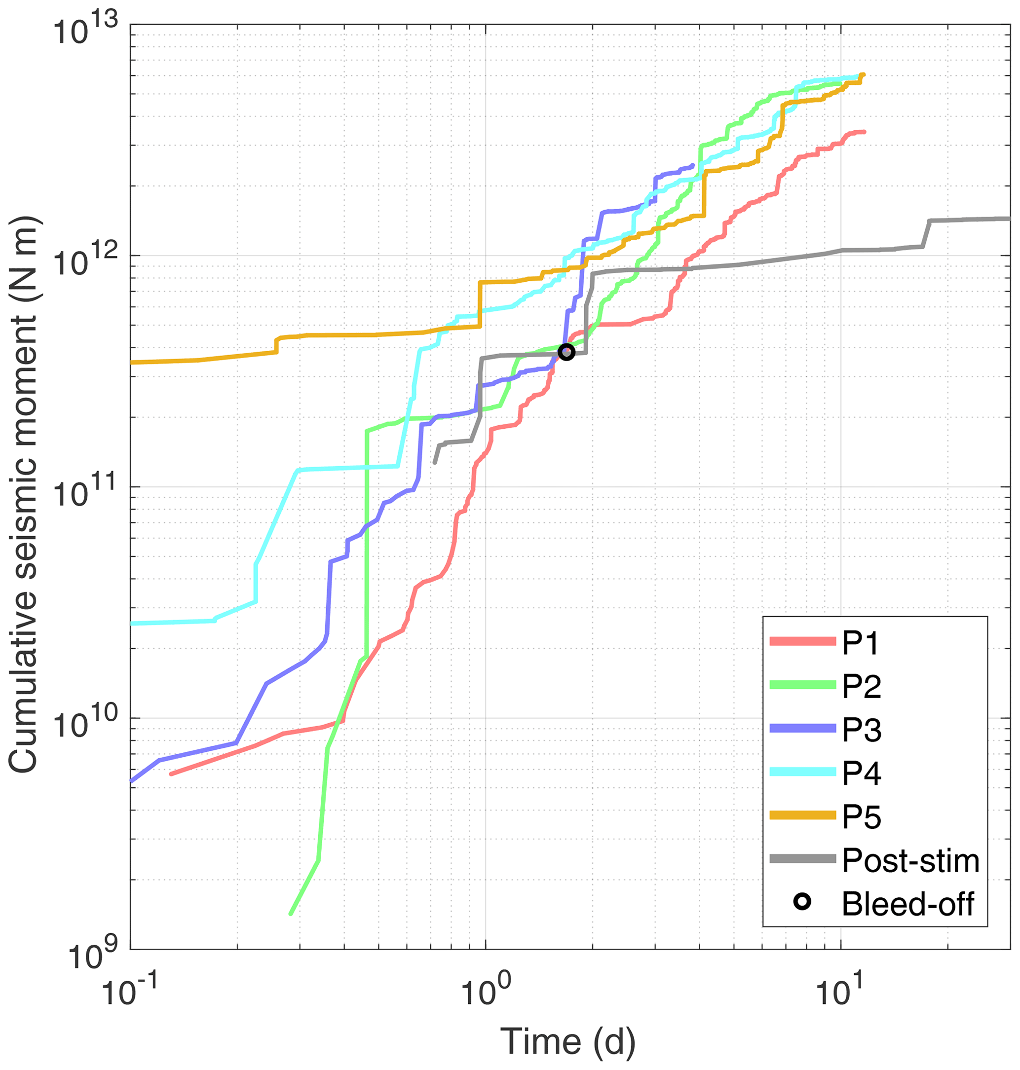
Figure 4 For a time period of 30 d, the temporal evolution of cumulative seismic moment release for the relocated seismicity is shown for each injection phase and for the post-stimulation phase.

The temporal evolution of the CM₀ separated for each hypocenter cluster, marked in Fig. 3b, is shown in Fig. 5. For the upper cluster, the increase in the CM₀ is visibly larger for the stimulation phase P1 than for the other phases. For stimulation phase P2, a substantial increase in CM₀ occurred between days 4 and 5. For the central hypocenter cluster, a substantial increase in the CM₀ is visible for stimulation phases P2, P4, and P5 at the beginning of day 3 and also for P1 and P4 during day 6. For both upper and central clusters, the post-stimulation CM₀ is substantially smaller compared to that from injection (Fig. 5a–b). The CM₀ during post-stimulation in the bottom cluster is similar to P2–P5 within the first 2 d and afterwards lower than P2–P5. Inevitably, the bottom cluster that hosts the majority of the seismic activity also displays the highest CM₀ (Fig. S2). We note that the slopes of the CM₀ evolution are similar for the upper and central cluster but steeper for the bottom cluster (Fig. S2).

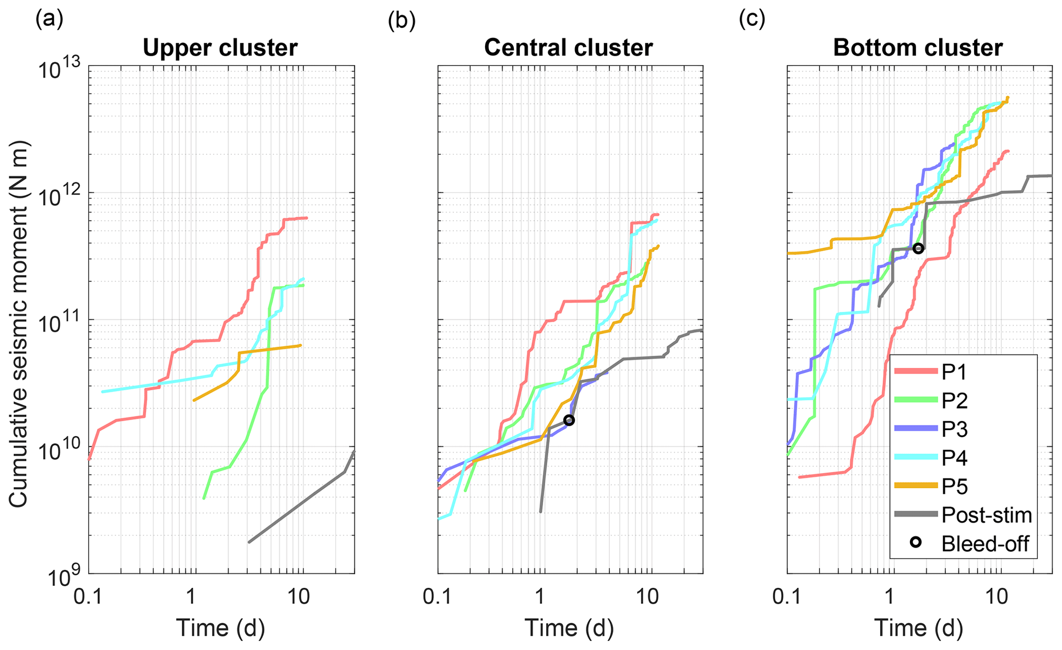
Figure 5 Temporal evolution of the cumulative seismic moment release with time for each of the three hypocenter clusters separately: (a) the uppermost hypocenter cluster, (b) the central hypocenter cluster, and (c) the deepest and main hypocenter cluster.

3.3 Spatial evolution of cumulative seismic moment

For the spatial distribution of the seismic moment, the area around the injection well was separated into horizontal bins of 50×50 m. The cumulative seismic moment of all events within each bin was then investigated by disregarding the depth. During stimulation, the largest moment release and level of seismic activity occurred at the center of the main event cluster at the bottom of the injection well close to the open-hole section (Fig. 6a–b). Furthermore, larger events in the main cluster tend to locate at the greatest depths. Interestingly, a NNW–SSE alignment of enhanced cumulative seismic moment release is visible in the main hypocenter cluster, in agreement with the preferred NW–SE-trending direction of the two upper hypocenter clusters. The hypocenters of larger events show a similar alignment (Figs. 6a, S3). A smaller area at the NNW outer flank of the bottom hypocenter cluster displays anomalously high CM₀ release caused by large events occurring during the last injection phases and after injection (red rectangle in Fig. 6a–b). Interestingly, epicenters of two tectonic seismic events with M_w 1.4 and M_w 1.7 were reported to occur in 2013 a few kilometers NW of the bottom-hole section of well OTN-3 (Kwiatek et al., 2019).

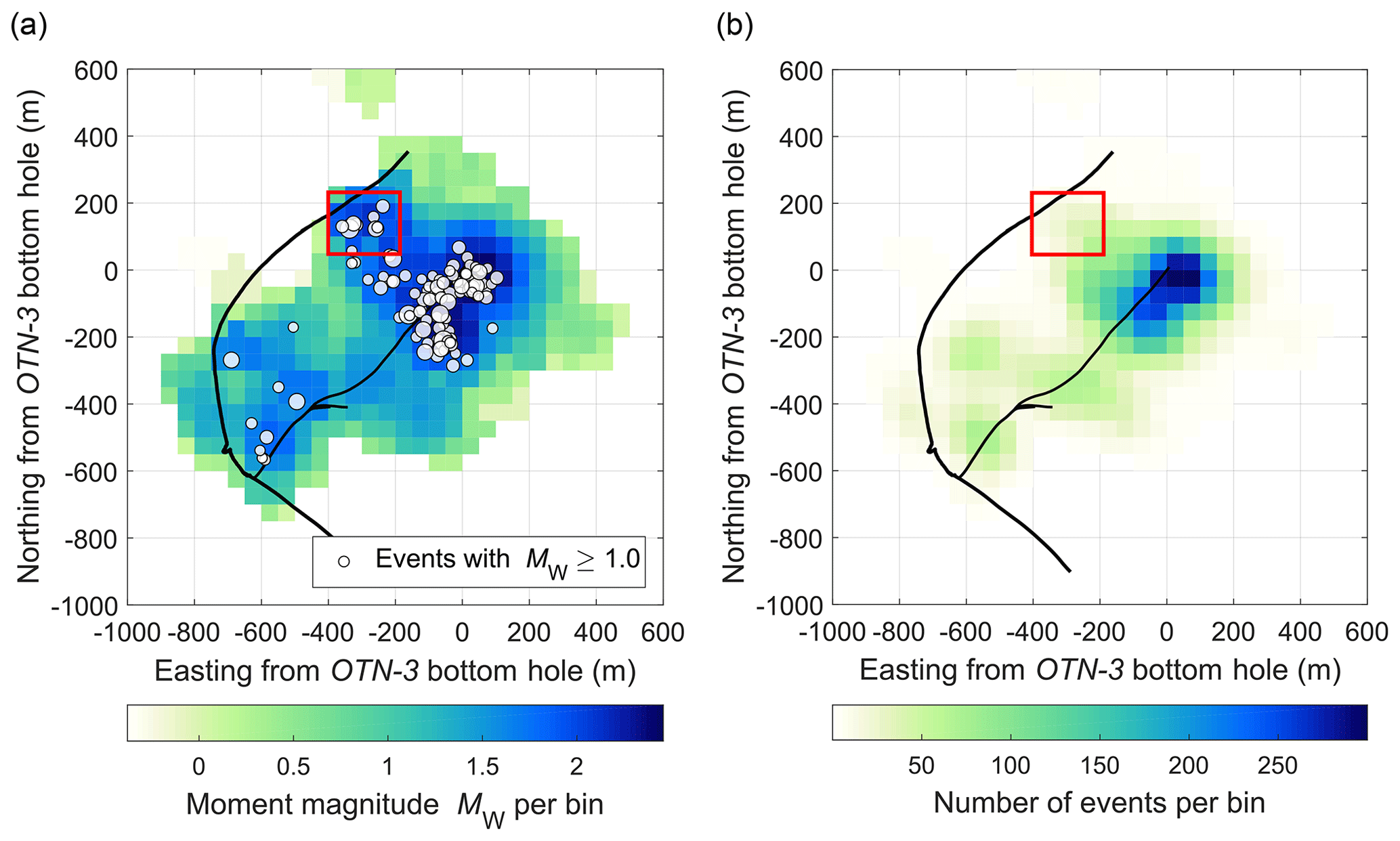
Figure 6 Spatial evolution of the cumulative seismic moment release of the relocated seismicity per bins of 50 by 50 m. (a) The cumulative seismic moment release converted to seismic moment magnitude per bin overlaid by seismicity with M_w≥1. (b) The number of events that occurred per bin. A smaller area of anomalously high CM₀ release caused by a few large events is highlighted by red rectangle.

3.4 Complexity of source mechanisms

We determined 191 single-event focal mechanisms (Fig. 7). Using the dendrogram tree based on hierarchical clustering (Fig. S4), events were separated into three distinct families (I–III) with similar focal mechanism orientations containing 99, 60, and 27 events, respectively (different coloring of beach balls in Fig. 7). Five events were not grouped into any of the three families and thus were not considered any further. Events belonging to the three families are not separated spatially. Oblique reverse faulting is the dominant source mechanism type, which is in contrast to the regional strike-slip regime (Kwiatek et al., 2019). The two largest events with reverse faulting were classified into family III. Fault plane solutions from all families indicate a range of preferred SSE–NNW to SW–NE strike directions, sharing comparable dips ranging approximately 35–50^∘ (Fig. 7a and e). The source mechanisms of only a few events indicate strike-slip faulting, with two of them occurring after shut-in. A total of 12 estimated focal mechanisms are post-stimulation events (Fig. 7b, d, and f). The post-stimulation events contained in the main hypocenter cluster at the bottom of the well have similar focal mechanisms as events during the stimulation. In the central hypocenter cluster, two strike-slip events occurred nearby.

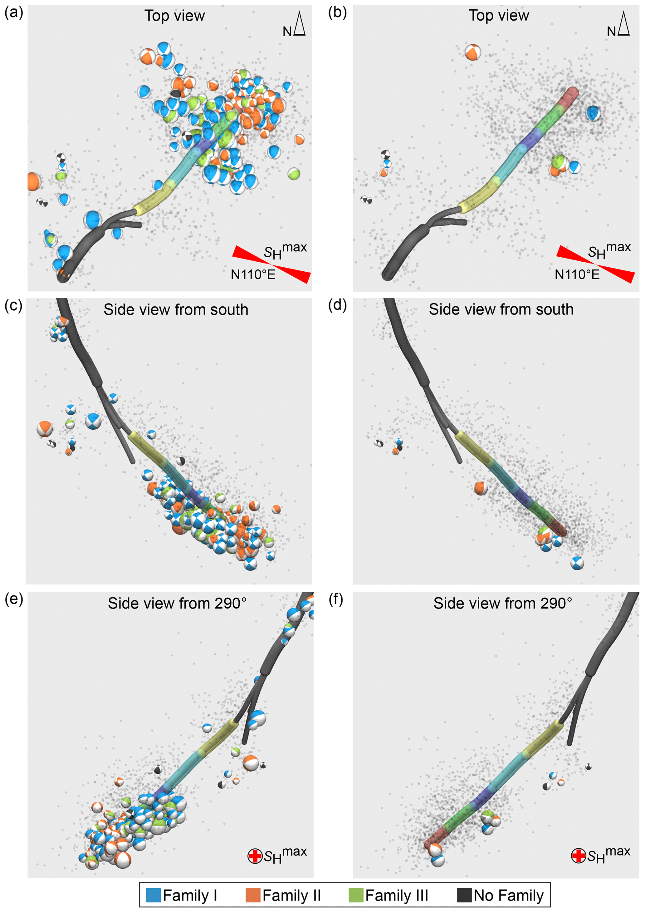
Figure 7 Orthogonal views of estimated focal mechanisms in three different projections: (a, b) map view, (c, d) side view from the south (180^∘), and (e, f) side view from the NW (290^∘) along the direction of the maximum horizontal stress $S_{\mathrm{H}}^{\max }=\mathrm{110}$^∘. (a, c, e) All 191 estimated focal mechanisms. (b, d, f) Focal mechanisms of post-stimulation events. The color code indicates the family obtained. Relocated seismicity without estimated focal mechanisms is plotted as small grey dots.

To further explore separation of the focal mechanisms into distinct families, we analyzed the rotation angle between the principal P and T axes as a measure of mechanism (dis)similarity. We first calculated the mean fault plane solution for each family. The strike, dip, and rake values of the mean fault plane solutions (FPSs) for the families are as follows: 332^∘, 47^∘, and 43^∘ for family I; 32^∘, 51^∘, and 141^∘ for family II; and 67^∘, 36^∘, and 122^∘ for family III, respectively. The focal mechanisms with mean fault plane solutions and all the best FPSs of each family are plotted in Fig. 8a–c. Hillers et al. (2020) recently estimated focal mechanisms for the 14 largest events, and the majority are similar to family I FMs. The calculated rotation angles between the mean solutions of families I and II, I and III, and II and III are 71, 59, and 53^∘, respectively. Taking into account that focal mechanisms are assumed to be similar if the Kagan rotation angle is less than 20^∘, none of the three families are similar to each other. The difference between families I and II is the most prominent, whereas rotations I–III and II–III are comparable. However, despite the mean solutions of different families being quantitatively distinct, the individual mechanisms are not necessarily very different (Fig. 8d–f) between families. The total P-axis uncertainties strongly overlap among the three families. At the same time, the T-axis uncertainties form three distributions that, when compared between families, only partially overlap. This overall suggests that the FPSs may be sensitive to changes in polarities at individual stations located close to the nodal plane.

Figure 8 (a–c) Mean fault plane solutions (black lines) calculated from the best FPSs of 99 events forming family I (a), 60 events forming family II (b), and 27 events forming family III (c). Contributing FPSs from which the mean is calculated are shown in blue, orange, and green, respectively. The most repetitive polarity pattern observed at each station is presented as a black or white dot for positive or negative onsets, respectively. P1 and P2 symbols correspond to the projections of the main and auxiliary fault planes according to which one is better oriented for failure on the Mohr circle represented in Fig. 10. (d–f) For each of the families, the mean P and T axes as well as axes of contributing FPSs are plotted as big and small white dots, respectively. The HASH-derived uncertainties (95 % confidence interval) of the P and T axis of all events within each family are shown using a blue and brown coloring scale, respectively.

In the following, we qualitatively analyze the polarity patterns of events forming three families. Regardless of whether the polarities are manually picked or estimated, the most repetitive polarity pattern observed at each station for a particular family is plotted in Fig. 8a–c. For each family and station, the percentage of FM events showing this repetitive pattern is presented in Table S1. We first verified the consistency of polarity patterns for events with manually picked polarities (N= 37, 15, and 15 FPSs for families I, II, and III, respectively). We noted that the strike-slip mechanisms are attributed to the least well-constrained focal mechanisms belonging to family II. The main substantial difference in the polarity patterns across families seems to be related to polarities observed at two stations, MALM and MUNK (Fig. 8a–c). For family I, the polarities at these two stations are negative and extremely consistent among events forming the family (35 out of 37 events display such a behavior). For family II, we observe MALM and MUNK to have a mostly negative and positive polarity pattern, respectively. For family III, the situation is reversed, with MALM and MUNK having a predominantly positive and negative polarity pattern, respectively. We further qualitatively analyzed the polarity pattern of events with polarities estimated from the cross-correlation-based technique of Shelly et al. (2016). Here, the situation is generally further complicated due to ambiguities in resolving the polarities because of a decreased signal-to-noise ratio. However, for the majority of the events forming family I, the resolved focal mechanisms still show a similar polarity pattern as the most repetitive pattern shown in Fig. 8a, with only incidentally changing polarities at stations UNIV and RUSK, which are both located further away from the EGS site than other sensors and thus display a lower signal-to-noise ratio. The pattern of resolved polarities for family II is generally comparable to the most repetitive polarity pattern shown in Fig. 8b. However, 18 out of 45 events have negative estimated polarities for MUNK; thus, the resolved polarity patterns seem to vary more in comparison to those of family I. The events with estimated polarities for family III have the same patterns for stations MALM and MUNK as the most repetitive pattern in Fig. 8c except for two events. However, other stations (e.g., UNIV, RUSK, and LASS) with a lower signal-to-noise ratio sometimes display varying resolved polarities for families II and III. We suppose that (1) the attribution of focal mechanisms to a particular family is substantially dependent on the polarity pattern of a limited number of stations that are located close to the nodal planes, and (2) family I focal mechanisms seem the most stable.

Using the BRTM and MSATSI stress tensor inversion methods based on 191 focal mechanisms, we estimated the local stress field orientation. The variability of FMs to constrain the stress field inversion is given due to high Kagan rotation angles between the mean FPSs of the three families with 53 to 71^∘. The BRTM results show that the maximum principal stress axis σ₁ is oriented almost horizontally, with a trend of 279^∘ and a plunge of 4^∘ (Fig. 9). The minimum principal stress axis σ₃ has a trend and plunge of 185^∘ and 67^∘, respectively. The trend of σ₁ and the stress shape ratio are comparable to their independent estimates using wellbore breakouts and minifrac shut-in pressures (see Backers et al., 2016; Kwiatek et al., 2019, for details), for which $S_{\mathrm{H}}^{\max }=$ N110^∘ E and R=0.46 were reported. Using the MSATSI method, the trend and plunge of σ₁ is calculated as 271^∘ and 11^∘, respectively. Thus, the estimated trend of σ₁ deviates ∼ 20^∘ from the maximum horizontal stress $S_{\mathrm{H}}^{\max }$. The minimum principal stress axis σ₃ is oriented with a trend of 76^∘ and a plunge of 79^∘. The estimated stress shape ratio is R=0.72, which is larger with respect to the BRTM and geophysical estimates.

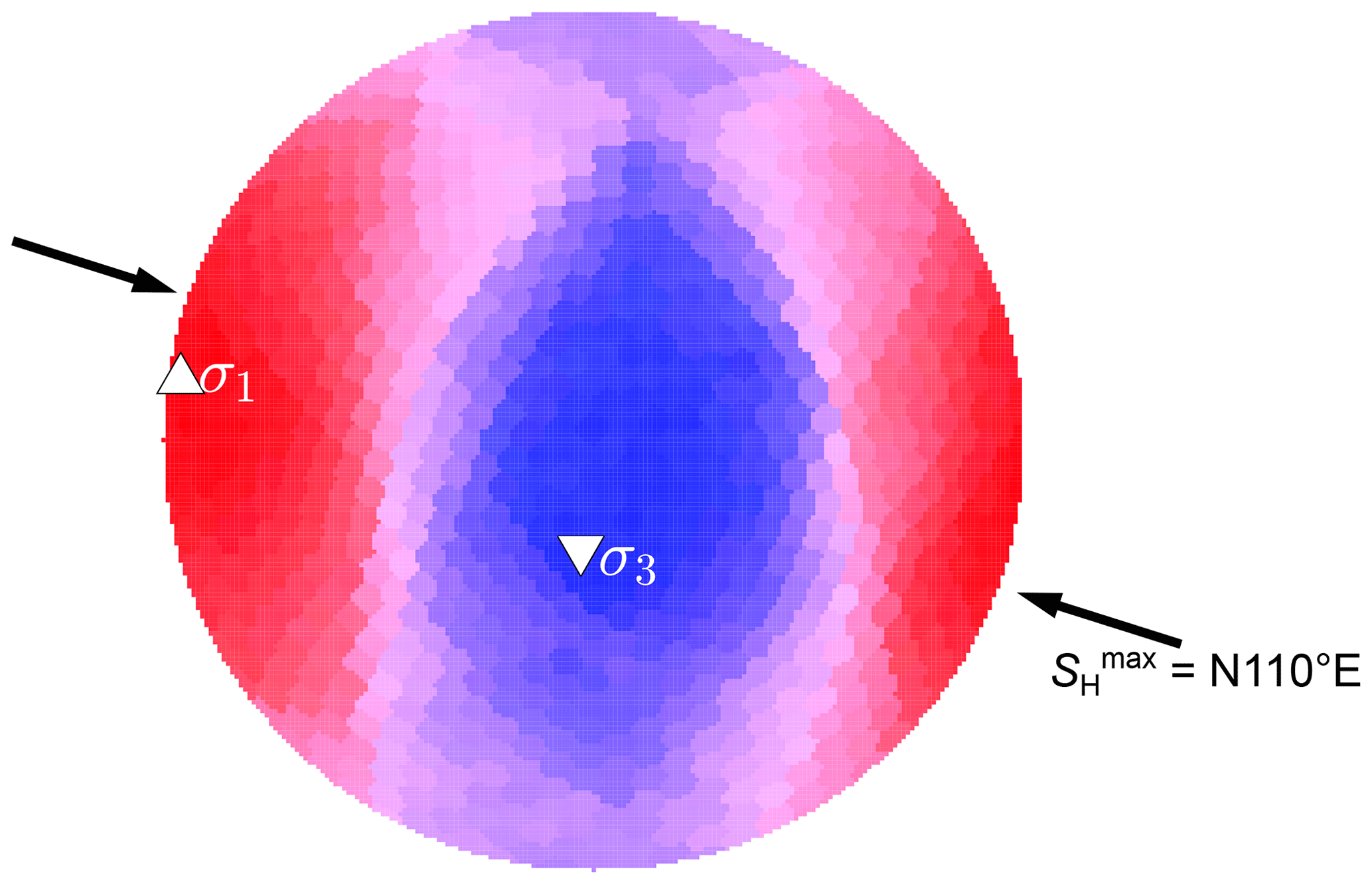
Figure 9 Stereonet of the estimated local stress field using the BRTM. White upward- and downward-pointing triangles represent maximum and minimum principal stress axes σ₁ and σ₃, respectively. Black arrows represent maximum horizontal stress $S_{\mathrm{H}}^{\max }$ in the reservoir.

The stress obtained by focal mechanism inversion represents a local reverse faulting regime. This is in contrast to the regional strike-slip regime estimated from regional stress and borehole data (Kwiatek et al., 2019). Only the focal mechanisms of a few events present a dominant strike-slip faulting, which are typically smaller events with a less well-constrained polarity pattern.

4 Discussion

Analysis of the seismic data suggests that fluid injection was performed into a complex network of small-scale pre-existing and distributed fractures and minor faults rather than activating a single major fault (Kwiatek et al., 2019). In an effort to characterize the structural complexity of the reservoir in detail, we compiled a high-resolution dataset of hypocenters and single-event focal mechanisms by enhancing and refining the original seismic catalog.

The relocated events of our updated catalog show three separated spatial hypocenter clusters along the injection well, in good agreement with Kwiatek et al. (2019) and Hillers et al. (2020). Hillers et al. (2020) used seismic data collected from an independent surface-based seismic network of dense sub-arrays, whereas Kwiatek et al. (2019) used the same seismic network as we do but a simplified velocity model and slightly different $V_P/V_S$ ratio. The hypocentral depths of the events vary slightly between this and previous studies. We found that differences between absolute locations among these catalogs are likely explained by variations in $V_P/V_S$ ratios and velocity models.

We also provide the first analysis of post-stimulation events, expanding the seismic catalog to investigate potential changes in the seismicity pattern from the stimulation to the post-stimulation period. Compared to the seismicity occurring during the stimulation, the post-stimulation seismicity shows no spatiotemporal migration. The largest post-stimulation events occurred at the NNW and SSE outer edges of the main hypocenter cluster where anomalously higher seismicity rates and larger events were also observed during the last stimulation phase P5 (see Fig. 3). For the main hypocenter cluster, the temporal evolution of the post-stimulation CM₀ shows similarities to the injection period until bleed-off of the well, with only small changes thereafter. This suggests that seismicity is driven by the elevated pressure in the reservoir due to the previous hydraulic pumping (increased stored elastic energy). However, hypocenter propagation requires active pumping. This is indicated by a much smaller residual increase in CM₀, no further migration of the seismicity after bleed-off, and a decrease in reservoir fluid pressure.

The spatiotemporal seismicity evolution during stimulation and the spatial distribution of the cumulative seismic moment release indicate clear alignment of the events in the NW–SE direction in the two shallower hypocenter clusters, which could signify activation of permeable zones along faults or joints oriented in this direction. The existence of these zones is supported by the results of OTN-3 well logging, wherein intervals of highly damaged rocks were detected that roughly coincide with the intersection of the upper seismicity clusters and the well path. For the largest bottom seismicity cluster, the relocated seismicity is distributed diffusively around the injection well. However, larger seismic events form a distinct alignment along a NNW–SSE direction (Figs. 6a, S3) with post-stimulation events clearly located at the perimeter of the narrow zone (Fig. S3). This alignment indicates activation of another permeable zone similar to the two upper ones. The NNW–SSE-trending orientation coincides with an abundance of very similar focal mechanisms from the best-constrained family I events with a strike direction nearly identical to the NNW–SSE alignment of hypocenters. Moreover, two natural micro-earthquakes with M_w 1.7 and M_w 1.4 occurred in 2013 a few kilometers NNW from the well (Kwiatek et al., 2019). Although there is no detailed information available on their depths due to limited coverage of the seismic network at their origin time, their epicentral location coincides with the NNW perimeter of the bottom NNW–SSE alignment hosting large induced seismicity events as well. These observations suggest that the stimulation activated at least three prominent NW–SE- to NNW–SSE-oriented permeable zones of sub-parallel fractures or faults that are responsible for seismicity migration away from the injection well during the stimulation. The deepest NNW–SSE-trending zone is buried in more disperse seismic activity forming the bottom cluster and hosts the largest induced earthquakes (and likely some natural at earlier times). The fact that the largest events occurred in the deepest permeable zone may simply be related to the highest expected pore pressure perturbation in this volume due to injection and migration of fluids. Kwiatek et al. (2019) speculated that the maximum event magnitude is either limited by available fault sizes or the strength of the faults. The total length of the NNW–SSE-trending permeable bottom zone (∼ 650 m, Fig. S3), clearly marked by the numerous and very similar focal mechanisms, is much larger than the average size of a single M_w 2 earthquake (∼ 80 m diameter) with even lower relocation precision. We therefore suggest that the upper limit on the maximum magnitude is related to the low fault strength.

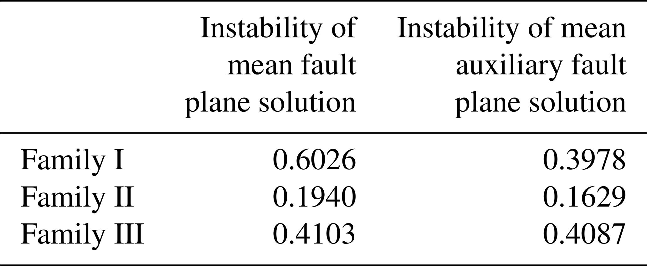
For the main hypocenter cluster, the seismicity migrates towards the NE and towards greater depths, dipping in the same direction as the inclined portion of the OTN-3 well (Fig. 3). The propagation of seismicity may signify activation of small-scale fractures striking NNW–SSE and dipping along the injection well. This is again supported by the catalog of source mechanisms forming family I events (see Figs. 7 and 8a). To further understand this striking observational and qualitative agreement of family I fault planes with spatial distribution and evolution of seismic activity, we tested which family of focal mechanisms is better oriented for failure within the local stress field estimated using the BRTM. The resulting BRTM stress tensor and estimated stress shape ratio R=0.53 have been used to create a Mohr diagram of the 3D stress state (Fig. 10) (see Vavryčuk, 2014; Martínez-Garzón et al., 2016). We projected estimated FPSs into the Mohr diagram, which revealed fault plane orientations with respect to the stress field. Optimally oriented fault planes, located generally closer to the left part of the Mohr diagram, are more likely to be activated (e.g., Vavryčuk, 2011), e.g., in the presence of enhanced pore fluid pressure. To quantify the proximity to failure criterion, we assumed a friction coefficient of μ=0.7 as a mean value for faults in the Earth's crust (Vavryčuk, 2011). While projecting the preferred fault plane out of the two nodal planes from each fault plane solution, we used the nodal plane that displayed a higher instability coefficient I (see Vavryčuk, 2014; Martínez-Garzón et al., 2016):

$$\begin{array}{}\text{(5)}& I={\displaystyle \frac{\mathit{\tau }+\mathit{\mu }({\mathit{\sigma }}_{\mathrm{n}}+\mathrm{1})}{\mathit{\mu }+\sqrt{\mathrm{1}+{\mathit{\mu }}^{\mathrm{2}}}}},\end{array}$$

with τ and σ_n as the normalized shear and normal tractions, respectively, and μ as the friction coefficient.

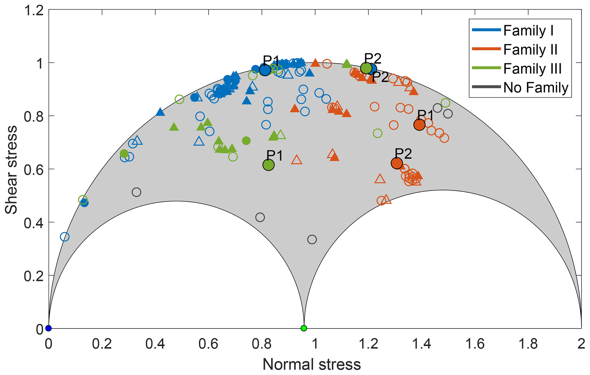
Figure 10 Deviatoric Mohr circle representing the local stress field, with the fault plane solutions having the highest fault instability coefficient of the estimated focal mechanisms. The stress inversion resulted in a stress ratio of R=0.53. Events with M_w≥1 and M_w<1 are plotted as triangles and circles, respectively. Filled and unfilled markers represent events with manually picked and estimated polarities, respectively. The mean and its auxiliary fault plane solution of each family are plotted as filled large dots labeled as P1 and P2, respectively. Most family I events (blue symbols) occurred on critically stressed faults.

Clearly, FPSs from family I are the most favorably oriented with respect to the local stress field (blue points and triangles in Fig. 10), as also indicated by the highest fault instability coefficients (Fig. 11). It turned out that the most optimally oriented fault plane is always the one trending NNW–SSE and dipping approximately in the direction of the inclined portion of the OTN-3 well (indicated by P1 nodal planes in Fig. 8a). This is also confirmed by the mean solution of family I (332^∘/47^∘ plane, blue P1 marker in Fig. 10) displaying the highest instability (Table 1). However, the fault planes represented by the auxiliary plane of the mean solution of family I are also quite favorably oriented (blue P2 marker in Fig. 10). Some of the family III events are also quite favorably oriented with the stress field. We note that instabilities in the auxiliary planes of mean FPSs for families I and III are similar (green and blue P2 dots in Fig. 10, Table 1), in agreement with their mean auxiliary nodal plane orientations of 210^∘ and 60^∘ (P2 in Fig. 8b–c). Qualitatively, nodal planes from family II seem to be mostly unfavorably oriented with the stress field (orange points and triangles in Fig. 10), as indicated by the lowest instability coefficients (Fig. 11). However, some P1 nodal planes strike N–S (see Fig. 8b) and thus show quite similar orientations as the P1 FPSs of family I (Fig. 8a), leading to higher instability coefficients for these planes (orange dots and triangles close to the blue and green P2 marker in Fig. 10). Here, we found 19 events of family II that show similar polarity patterns as those observed for family I events, with an opposite polarity only for station MUNK.

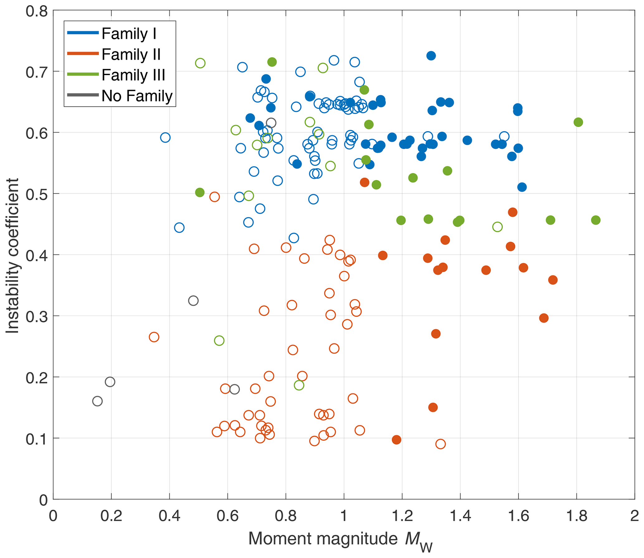
Figure 11 Highest fault instability coefficient of any of the two FPSs for each FM event plotted with moment magnitude. Events with manually picked and estimated polarities are plotted as filled and unfilled circles, respectively.

Table 1 Fault instabilities of the mean fault plane solution and its auxiliary plane for each family.

The performed analysis of fault instability clearly showed that high-quality focal mechanisms constituting family I events display a comparable oblique reverse component and optimally oriented fault planes striking approximately NNW–SSE and dipping around 45^∘. These fault plane orientations are in agreement with the estimated stress field, and they explain the spatiotemporal evolution of seismicity well with the corresponding fluid migration pattern. The 2018 seismicity activated a pre-existing network of small-scale parallel fractures dipping to the ENE, in agreement with the dip direction of the inclined part of the injection well. Fault planes striking NNE–SSW to NE–SW and dipping around 60^∘ were also indicated to be quite favorably oriented with the stress field represented by the auxiliary plane of the mean FPSs for families I and III. Drill bit seismic data suggest the existence of a steeply dipping NE–SW-striking structure, which might have been activated by the 2018 seismic activity. We note that the FM results are in good agreement with a limited number of 14 focal mechanisms of the strongest events presented in Hillers et al. (2020), with all but one displaying reverse faulting motions.

5 Summary and conclusions

We present a new seismic catalog for the geothermal stimulation in Helsinki 2018, by determining new locations and relocations on the basis of the new VSP-based velocity model, and include the post-stimulation seismicity, resulting in a catalog with 5456 events. The catalog is extended by the list of detections, amounting to 61 163 events provided to the scientific community (see Leonhardt et al., 2021). The magnitude of completeness of the entire catalog is $M_{\mathrm{c}}=-\mathrm{1.10}$. The catalog is supplemented by 191 focal mechanisms, calculated using polarity-based and cross-correlation-based methods, and is used to discuss the structural complexity of the reservoir.

Spatial migration of the seismicity is driven by enhanced pore fluid pressure due to active injection, as no spatial migration of the post-stimulation seismicity after bleed-off is found. Until shortly after the bleed-off, the increase in the cumulative moment release of the post-stimulation seismicity with time is comparable to the slope of the CM₀ during individual stimulation phases but substantially less afterwards. This is especially observed for the seismicity of the deepest hypocenter cluster.

An activated network of at least three NW–SE- to NNW–SSE-oriented fracture zones of up to 200 m thickness seems to be responsible for the significant seismic activity migration towards the NW–NNW and SE–SSE away from the injection well. The deepest fracture zone also hosts many of the larger seismic events with magnitudes exceeding M_w≥1; this suggests elevated fluid volume and pore fluid pressure, leading to the accumulation of hydraulic energy in this area that is relaxed in larger seismic events.

The best-constrained focal mechanisms strike NNW–SSE, in agreement with the orientation of three fracture zones. Most of these mechanisms display ∼ 45^∘ ENE-dipping oblique thrust-fault planes that were found to be critically stressed in the resolved local stress field. These fault kinematics explain the NNW–SSE migration of seismicity well along damage zones, in addition to the downward migration of events towards the NE–NNE along the dip direction vector of the inclined portion on the injection well.

We conclude that seismic slip occurs on a sub-parallel network of favorably oriented pre-existing but weak fractures striking in the NNW–SSE direction and dipping 45^∘ ENE. The localization of seismic moment release in NNW–SSE-trending zones suggests the existence of NNW–SSE-trending damage structures or lithological differences that increase the mobility of fluids in confined parts of the reservoir.