the Creative Commons Attribution 4.0 License.
the Creative Commons Attribution 4.0 License.
 | 19 Mar 2021
Gravity effect of Alpine slab segments based on geophysical and petrological modelling
Jörg Ebbing
Amr El-Sharkawy
Thomas Meier
In this study, we present an estimate of the gravity signal of the slabs beneath the Alpine mountain belt. Estimates of the gravity effect of the subducting slabs are often omitted or simplified in crustal-scale models. The related signal is calculated here for alternative slab configurations at near-surface height and at a satellite altitude of 225 km.
We apply three different modelling approaches in order to estimate the gravity signal from the subducting slab segments: (i) direct conversion of upper mantle seismic velocities to density distribution, which are then forward calculated to obtain the gravity signal; (ii) definition of slab geometries based on seismic crustal thickness and high-resolution upper mantle tomography for two competing slab configurations – the geometries are then forward calculated by assigning a constant density contrast and slab thickness; (iii) accounting for compositional and thermal variations with depth within the predefined slab geometry.
Forward calculations predict a gravity signal of up to 40 mGal for the Alpine slab configuration. Significant differences in the gravity anomaly patterns are visible for different slab geometries in the near-surface gravity field. However, different contributing slab segments are not easily separated, especially at satellite altitude. Our results demonstrate that future studies addressing the lithospheric structure of the Alps should have to account for the subducting slabs in order to provide a meaningful representation of the geodynamic complex Alpine area.
- Article
(4672 KB) - Full-text XML
- BibTeX
- EndNote


Interpretation of gravity anomalies can reveal information on the architecture and tectonic setting of the lithosphere (e.g. Zeyen and Fernàndez, 1994; McKenzie and Fairhead, 1997; Holzrichter and Ebbing, 2006; Braitenberg, 2015; Spooner et al., 2019). For subduction zones, like the Andes, several studies have shown that the gravity effect of the subducting plates is significant and has to be considered in order to study the feedback between the subducting lithosphere and the overriding plate (Götze et al., 1994; Götze and Krause, 2002; Tašárová, 2007; Gutknecht et al., 2014; Götze and Pail, 2018; Mahatsente, 2019). For lithosphere to subduct, a higher density than the surrounding mantle material at the same depth interval is required, causing a negative buoyancy for the slab, and therefore the slab is subducted into Earth's interior (e.g. Kincaid and Olson, 1987; Ganguly et al., 2009). However, the gravitational contribution of subducting material in the upper mantle to the gravity field has so far not been systematically addressed for the Alpine system. In order to provide an assessment, the magnitude of the gravity signal of such subcrustal long wavelength features has to be estimated.
The Alpine mountain belt (Fig. 1a) is chosen for this sensitivity study because firstly a large range of recent seismic tomography studies imaged subducting slab segments in the Alpine region (e.g. Babuška et al., 1990; Lippitsch et al., 2003; Spakman and Wortel, 2004; Mitterbauer et al., 2011; Karousová et al., 2013; Zhao et al., 2016; Kästle et al., 2018; El-Sharkawy et al., 2020). Those different studies suggest different configurations of slab segments (see Sect. 1.1), allowing us to test how sensitive the gravity field is to varying geometries of subducting slab segments. Secondly, previous Alpine models addressing the Alpine gravity field have considered the subcrustal mantle inhomogeneities in the form of lithosphere thickness (e.g. Ebbing et al., 2006; Spooner et al., 2019) or in the form of mantle density variations (Tadiello and Braitenberg, 2021) but without identifying the isolated effect of subducting slabs segments in the velocity or density variations. If the contribution of the mantle density variations is not considered, a significant part of the gravity field might be attributed to crustal thickness variations or intracrustal sources.
In addition, the Bouguer anomaly of the Alps (Fig. 1b) shows no direct sign of subducting slabs (in contrast to the Andes subduct zone) as the field is dominated by crustal thickness variations (Ebbing et al., 2001, 2006). Therefore, forward modelling of the proposed slab geometries, as imaged by high-resolution tomographic studies, is necessary to separate the gravity signal caused by the subducting slabs from the gravity anomaly field.
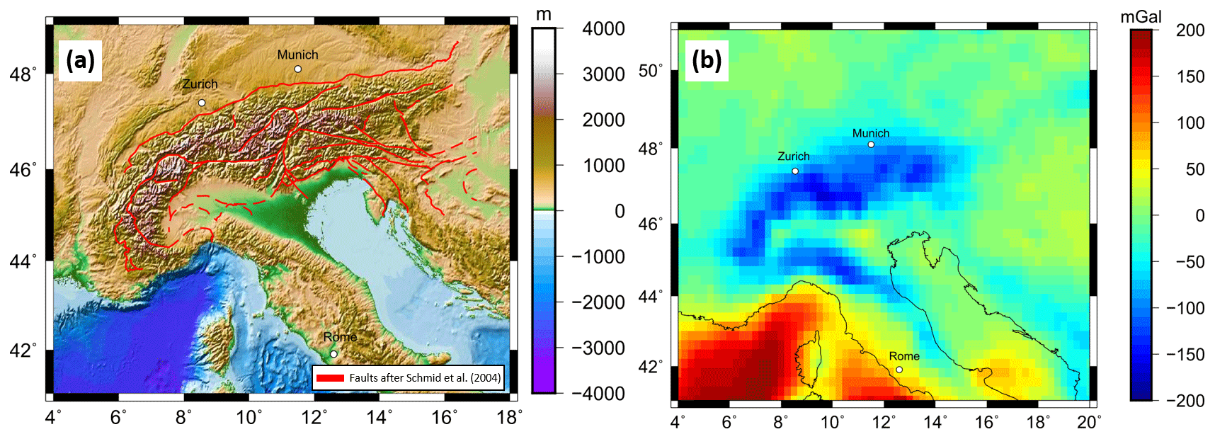
Figure 1(a) Topography from ETOPO1 from Amante and Eakins (2009), with faults in red after Schmid et al. (2004). (b) Bouguer anomaly based on XGM 2019 (Zingerle et al., 2020) with a maximum spherical harmonics degree of 719 at a station height of 6040 m above the ellipsoid, just above the surface of the Alps. Correction density for rock: 2670 kg m−3; and for water: 1030 kg m−3.
We present three different approaches to model the gravity effect of the slab segments and discuss the strengths and limitations of the applied methods. In the first approach, the Alpine subcrustal density distribution is derived by converting seismic velocities to density. This model is then forward calculated to estimate the gravity response. In the second approach, 3-D slab geometries are derived by evaluating seismic crustal thickness estimations and high-resolution upper mantle tomographic models. Here, two competing slab configurations are chosen. The predefined slab geometries are then forward calculated by assigning different density contrasts and slab thicknesses. The third approach uses similar predefined slab configurations to those in the second approach; however, here, we consider petrology, temperature and density variation. The gravity response is calculated for all three approaches at a near-surface height for the gravity disturbance and the gravity gradients at a satellite altitude of 225 km.
Alpine setting
The formation and present geodynamics of the Alps are linked to long-lasting tectonic processes, including Adria–Europe continent–continent collision, subduction of the oceanic and continental lithosphere, the formation of crustal nappes as well as extensional and shortening processes (Frisch, 1979; Stampfli and Borel, 2002; Handy, et al., 2010, 2015). The Adriatic microplate is a major driver of the present geodynamics in the Alpine region, which is trapped between the converging major plates of Europe and Africa. Adria is moving anti-clockwise with respect to Europe, as seen by GPS observations (e.g. Nocquet and Calais, 2004; Vrabec and Fodor, 2006; Serpelloni et al., 2016) and is subducted beneath the Apennines to the west as well as to the east beneath the Dinarides, while colliding with Eurasia in the Alps to the north (e.g. Channel and Horvath, 1976; Dewey et al., 1989; Stampfli and Borel, 2002; Handy et al., 2010; Le Breton et al., 2017). Subducting slab segments have been imaged by different seismological body wave travel-time tomographic studies as well as surface wave tomographic studies within the Alpine upper mantle (e.g. Babuška et al., 1990; Lippitsch et al., 2003; Spakman and Wortel, 2004; Mitterbauer et al. 2011; Karousová et al., 2013; Zhao et al., 2016; Kästle et al., 2018; El-Sharkawy et al., 2020). However, the configuration of subducting slab segments remains controversial. In the Western Alps, Lippitsch et al. (2003) propose a slab break-off at about 100 km depth, which is in line with the findings of Beller et al. (2018), Kästle et al. (2018) and El-Sharkawy et al. (2020). In contrast, a continuous subducting slab segment in the Western Alps, down to at least 250 km depth, is imaged by a number of other tomographic models (e.g. Koulakov et al., 2009; Zhao et al., 2016; Hua et al., 2017; Lyu et al., 2017).
A continuous subduction of Eurasia beneath the Central Alps down to at least 200 km depth is imaged by different tomographic models (e.g. Lippitsch et al., 2003; Piromallo and Morelli, 2003; Koulakov et al., 2009; Mitterbauer et al., 2011; Hua et al., 2017; Fichtner et al., 2018; El-Sharkawy et al., 2020). A potential slab gap with an approximate size of 2∘ is separating the subducting slab segments in the Central Alps to the Eastern Alps as imaged by, e.g. Lippitsch et al. (2003). The slab configuration and subduction direction in the Eastern Alps remains unclear. According to the classical view, Eurasia is subducting beneath Adria in a southward subduction (Hawkesworth et al., 1975; Lüschen et al., 2004, 2006). This idea was challenged by Lippitsch et al. (2003), Schmid et al. (2004), Kissling et al. (2006), Handy et al. (2015) and Hetényi et al. (2018). Instead, slab break-off in the Eastern Alps and a northward-dipping Adriatic slab in the easternmost Alps is suggested, leading to a switch of the slab polarity, as Adria is subducting beneath the European plate (Handy et al., 2015). The view that Adriatic and not Eurasian lithosphere is subducting northwards in the Eastern Alps has been opposed by Mitterbauer et al. (2011), as their model shows a northward-dipping slab in the eastern most Alps connected to the European plate. In an early tomographic study, Babuška et al. (1990) proposed that both Eurasian and Adriatic lithosphere is subducting in the Eastern Alps. In subsequent studies and interpretations, this model was mentioned but northward subduction of Adria seems to be favoured (e.g. Karousová et al., 2013; Hetényi et al., 2018). Recently, subduction of both Eurasian and Adriatic lithosphere in the Eastern Alps down to about 150 km has been suggested by Kästle et al. (2020) and El-Sharkawy et al. (2020) based on surface wave studies. For a more in-depth comparison and discussion of tomographic Alpine models, the reader is referred to, e.g. Kästle et al. (2020).
The Bouguer anomaly (Fig. 1b) is based on the XGM 2019 global model (Zingerle et al., 2020) developed for spherical harmonics up to degree 719, with a resolution of ∼ 25 km (half wavelength). The XGM 2019 model is a global integrated gravity model, which includes satellite and terrestrial measurements. The Bouguer anomaly is calculated from the free-air gravity disturbance with a correction density of 2670 kg m−3 for topography and a correction density for water of 1030 kg m−3 for the offshore areas using Tesseroids (Uieda et al., 2016). For the Tesseroids, we use the topography and bathymetry from ETOPO (Amante and Eakins, 2009), which was regridded at a regular grid with a grid space of 25 km to match the resolution of the XGM 2019 model for a maximum degree of 719. The gravity field is defined at a constant station height of 6040 m above the ellipsoid, just above the surface of the Alps. The resulting Bouguer anomaly shows a gravity low on the order of −200 mGal over the high topography of the Alps, indicating an isostatic crustal thickening in response to topography (e.g. Ebbing et al., 2006). Additionally, we calculate the mass correction for the gravity gradients at a station height of 225 km representing the Gravity field and steady-state Ocean Circulation Explorer (GOCE) satellite altitude. The topographic corrected gravity gradients after Bouman et al. (2016) measured by the GOCE European Space Agency (ESA) satellite mission are presented in the Appendix.
For the definition of the slab geometry, we use crustal thickness estimates based on the receiver function study by Spada et al. (2013). The crustal thickness map was digitized and the Moho gap in the Eastern Alps is filled by nearest-neighbour interpolation. To avoid edge effects, surrounding areas are supplemented by the Moho depth model of the European plate by Grad et al. (2009); both data sets were merged using a cosine taper with a taper width of 2∘ using Eq. (1). The overlapping areas at the grid edges are distance weighted to obtain a smooth transition.
with , with .
The merged Moho depth map is sampled at a regular grid with a cell size of 0.25∘ (Fig. 2) to be consistent with the resolution of the topographic and gravity models.
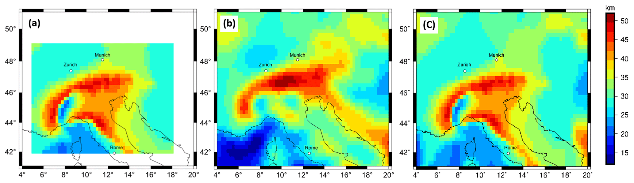
Figure 2(a) Digitized Moho depth after Spada et al. (2013) with a 0.25∘ grid spacing. (b) Moho depth estimation after Grad et al. (2009) with a 0.25∘ grid spacing (c) merged Moho depth map from Spada et al. (2016) and Grad et al. (2009) with a grid resolution of 0.25∘ using a cosine taper with a 2∘ width.
For the upper mantle seismic velocity, the 3-D shear-wave velocity model (MeRE2020) by El-Sharkawy et al. (2020) is used (Fig. 3). The model covers the upper mantle across the Alpine–Mediterranean area down to a depth of 300 km, and absolute shear-wave velocities are given.
In this study, relative shear-wave velocities in the depth range from 70 to 200 km are calculated with respect to a 1-D average shear-wave velocity model; the background model is described in El-Sharkawy et al. (2020). The upper limit of 70 km is introduced because (i) we focus on the contribution of the slab segments therefore removing crustal information from the model; (ii) the MeRE2020 tomography model is not sensitive to shallow structures – as a result, the slabs are not well recovered in depths shallower than 70 km; (iii) we want to ensure a uniform upper boundary. The lower boundary of 200 km is chosen based on clear images of the Alpine slab segments to at least 200 km depth (with the exception of the Western Alpine slab), as discussed in Sect. 1, and the assumptions that depth larger than 200 km will have a negligible effect on the regional gravity field considered here.
The ambient noise tomography by Kästle et al. (2018) is used to define the geometry of the Western Alpine slab segment; hence, we follow the idea of a slab break-off in the Western Alps at 100 km depth (Kästle et al., 2020), as suggested also by Lippitsch et al. (2003) and Beller et al. (2018). For the Eastern Alps, we consider two alternative models. For the first hypothesis, the P-wave tomography by Lippitsch et al. (2003) is used to define the Eastern Alpine slab segment. The second hypothesis is based on Kästle et al. (2020) and El-Sharkawy et al. (2020). It assumes southward subduction of a short Eurasian slab as well as northward subduction of a short Adriatic slab in the Eastern Alps. The slab configurations which are incorporated in the Alpine density models are discussed in greater detail in Sect. 4.1.
Seismic velocity variations are dependent on temperature and pressure. Densities in the subsurface are also temperature and pressure dependent. A conversion factor (ζ) can describe the linear relation between seismic velocities variations and densities variation (e.g. Tiberi et al., 2001; Webb, 2009). We convert seismic shear-wave velocities from the MeRE2020 tomographic model by El-Sharawy et al. (2020) in the depth range from 70 to 200 km, as discussed in Sect. 2, to obtain a density distribution of the upper mantle in the Alpine region based on a conversion factor (ζ). The relationship between seismic velocities and densities is described in Eq. (2); this assumption is a strong simplification of reality but gives a first-order estimation of the expected relative density structure beneath the Alps.
with Vsvabs the absolute velocities from MeRE2020, Δ% the percentage deviation from the MeRE2020 background model and ζ the conversion factor.
The result is strongly dependent on the chosen conversion factor. A range for conversion factors has been proposed in the literature for different rock types ranging from 0.1 to 0.45 (e.g. Isaac et al., 1989; Isaak, 1992; Karato, 1993; Kogan and McNutt, 1993; Vacher et al., 1998). The relative shear-wave velocity distribution in a 3-D domain from the MeRE2020 tomography model from El-Sharkawy et al. (2020) is converted using a constant conversion factor (ζ) of 0.3. The converted relative density distribution varies between −240 and 350 kg m−3. High correlations between the structural pattern in the converted density distribution and the relative seismic velocities are observed (Fig. 3), the similarity in the structure pattern is expected due to the linear relationship we introduced here. The converted 3-D relative density distribution reflects the variation of seismic velocities in the Alpine lithosphere and therefore includes the heterogeneities of the subduction slab segments, as seen by the tomographic models (Fig. 3). The relative density model is transferred into Tesseroids with a horizontal expansion of 0.2∘ and a vertical expansion of 3 km. The Tesseroid model is forward calculated in order to estimate the gravity response of the converted density distribution of the Alpine lithosphere in the depth interval of 70 to 200 km. No horizontal extensions of the mantle model are introduced because relative densities are used, and therefore edge effects are not expected to be significant and would only affect the outer most degrees of the model. The slab segments are located central in the model far away from possible artefact due border effects.
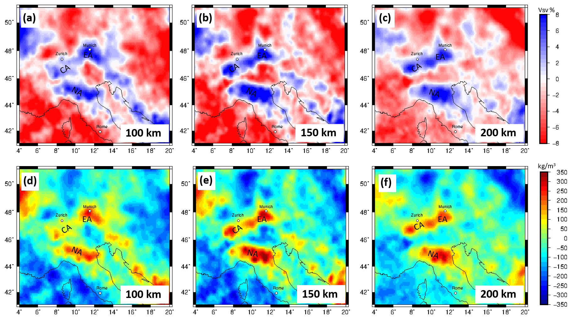
Figure 3(a–c) Depth slices of relative surface wave velocities (Vsv) from MeRE2020 (El-Sharkawy et al., 2020). (d–f) Converted relative density distribution in different depths based on a conversion factor (ζ) of 0.3. CA – Central Alpine slab; EA – Eastern Alpine slab; NA – Northern Apennine slab.
Results
In the forward-calculated gravity field, a gravity high with a magnitude of ∼ 40 mGal is observed over the Alps (Fig. 4). That might be interpreted as relating to the proposed slab segments in the Northern Apennine and Alpine area. However, the gravity field (and gradients; see the Appendix) is dominated by anomalies outside the Alpine realm (Fig. 4), for instance, in the Ligurian Sea and the Dinarides–Hellenides orogen. Therefore, in the next step, we try to concentrate on the seismic anomalies in the Alpine realm that can be related to the slab segments.
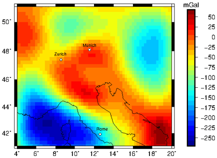
Figure 4Forward-calculated gravity signal from relative density distribution converted from relative seismic velocities using a conversion factor of 0.3 at a station height of 6040 m.
To estimate the gravity contribution of independent slab segments, we introduce different models for the subducting lithosphere. First, we use a set of models with simple constant density distribution in the slab, where the parameters, namely the density contrast and thickness of the slab segment is varied (approach 2). Secondly, we create a set of slab models accounting for compositional and thermal variations with depth (approach 3). Those models of approach 3 are created with the LitMod3D software package (Fullea et al., 2009), and here the slabs are strictly vertical due to software limitations. Slab models created within LitMod will be referred to as LitMod models in the following. For all non-LitMod models, the gravity and gravity gradients are calculated using Tesseroids, which are spherical prisms (Uieda et al., 2016).
4.1 Slab modelling with constant density contrast and slab thickness
We define two alternative slab configurations based on crustal thickness model by Spada et al. (2013) and several different tomographic studies; see a detailed description of the slab configurations below. At different depths, isolines are picked in the Moho depth map and tomographic images, defining the upper boundary of subducting slab segments. The isoline of the crust mantle boundary (Moho interface) is used as an onset of the slab to the crust and defines the upper boundary of the subduction slab segment. At upper mantle depth, increased seismic velocity anomalies in tomographic models beneath the Alps are interpreted as contrast between colder and therefore denser subducting material to the surrounding mantle material. At 100, 150 and 200 km depths, the upper boundary of the slab segment is defined at the 0 % contour line of the relative seismic velocity, marking the transition from rocks with low velocity to high-velocity rocks. The isolines at the Moho interface (100, 150 and 200 km depths) are displayed upon the Alpine topography (Fig. 5a–b). Vertical interpolation between the upper boundary isolines at different depths (Moho depths of 100, 150 and 200 km) defines a continuous surface of the upper slab boundary. The lower boundary of the slabs, and therefore the thickness of the slab segment, is not picked based on seismic data but assumed to have constant thicknesses for simplifications. The thickness is varied for different models from 60 to 100 km depth.
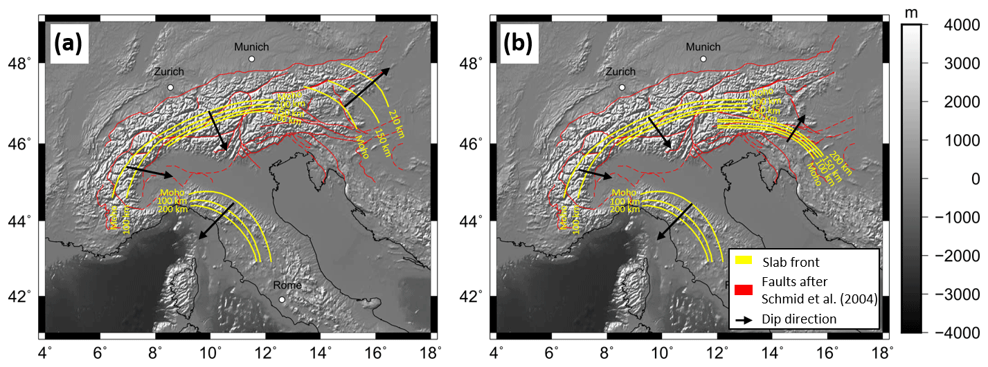
Figure 5Defined isolines based on crustal thickness estimations and seismological tomography models for the upper slab boundary for (a) Configuration 1 and (b) Configuration 2. Black arrows indicate the subduction direction. The fault configuration after Schmid et al. (2004) is shown in red.
4.1.1 Alternative slab configurations
We define two different slab configurations. Configuration 1 (Fig. 5a) features a northeast-subducting slab segment in the Eastern Alps based on Lippitsch et al. (2003). A Central Alpine slab segment is defined based on Lippitsch et al. (2003) and MeRE2020 (El-Sharkawy et al., 2020) subducting in south–southeast direction. The Eastern and Central Alpine slab segments are separated by a slab gap and show perpendicular subduction directions. The east–southeastward subducted slab segment in the Western Alps is defined using the tomographic model of Kästle et al. (2018), supporting the idea of slab break-off at about 100 km depth. Only attached slab segments are considered, ignoring potential mantle upwelling in the break-off zone and neglecting the potentially remaining detached slab segment in larger depths. In addition, a southwest-subducting slab segment beneath the northern Apennines is considered down to about 200 km depth, as imaged by MeRE2020 (El-Sharkawy et al., 2020) because of its proximity to the Western Alps.
Configuration 2 (Fig. 5b) considers a slab configuration mainly based on the interpretation of the MeRE2020 model (Fig. 3) by El-Sharkawy et al. (2020). In the Eastern Alps, both a short southward-subducting Eurasian slab segment as well as a short northward-subducting Adriatic slab are assumed. The Central and Western Alpine slab segments as well as the slab beneath the northern Apennines are identical to Configuration 1.
4.1.2 Forward calculation
To estimate the gravity effect of the slab configurations, the geometries are discretized into Tesseroids with a 0.2∘ extension in the horizontal domain and a vertical size of 20 km. The Tesseroids range from 40 to 200 km depth. First, a constant density contrast is assigned to the entire slab. We test density contrasts from 20 to 80 kg m−3. The thickness of the Alpine slab is not well constrained. We test for three slab volumes by assigning three slab thicknesses (60, 80 and 100 km) based on studies of other subducting slab segments (e.g. Wang et al., 2020). Due to the curved geometries of the proposed slab segments, rectangular Tesseroids with a horizontal expansion of 0.2∘ will either over- or underestimate the volume of a subducting slab at the edges of the slab. The percentage volume share of each Tesseroid to the slab geometry is calculated. The assigned density contrast of the Tesseroids which does not lay fully within the slab geometry is decreased according to the percentage volume within the slab geometry. Therefore, the density distribution correlates to the hypothetical slab positions and volumes in the Alpine subsurface without increasing the discretization resolution of the Tesseroid model beyond the uncertainty of gravity measurements and seismic tomographies. The offset between the 40 km upper Tesseroid boundary to the slab onset at the crust at 44 km depth is corrected using the same process.
4.1.3 Results
Forward-calculated slab models for predefined slab geometries of Configurations 1 and 2 with a constant density contrast of 60 kg m−3 and a constant thickness of 80 km result in a sharp gravity signal ranging from 70 to 100 mGal (Fig. 6). Both models generate gravity signals on the order of magnitude of 70 mGal in the Central Alpine region as well as in the Apennines. The gravity signal in the Eastern Alps differs for the two hypotheses (Fig. 6a, b). The Western Alpine slab segment shows the weakest signal in both models.
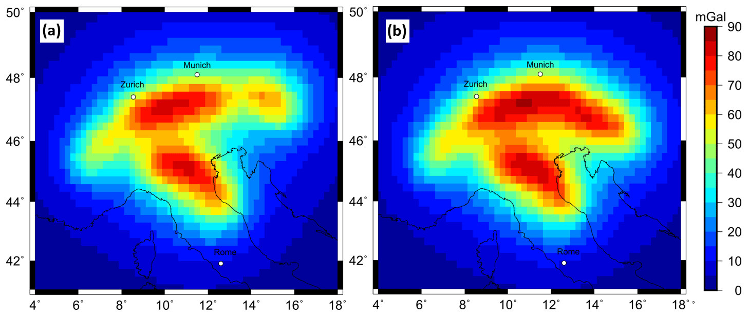
Figure 6Forward-calculated gravity disturbance signal at a station height of 6040 m for predefined subcrustal slab geometries with a content density contrast of 60 kg m−3 and a constant thickness of 80 km. (a) Predefined slab Configuration 1. (b) Predefined slab Configuration 2.
The gravity signal ranges from 30 to 110 mGal depending on the assigned density contrast and thickness for both slab geometry models (Fig. 7). The highest magnitude of the forward-calculated gravity signal is on the order of 110 mGal and is observed for a slab model with a density contrast of 80 kg m−3 and a constant slab thickness of 100 km, while the lowest signal is produced by a combination of 20 km m−3 density contrast and a slab thickness of 60 km. Similar gravity response is produced by different combinations of density contrast and volume. The signal pattern is influenced by the predefined slab geometry, while the magnitude of the gravity signal depends on the density contrast and thickness (Fig. 7).
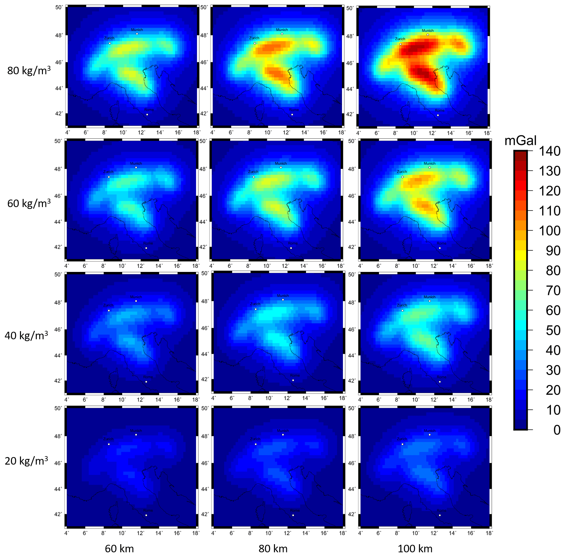
Figure 7Forward-calculated gravity disturbance signal for 12 different combinations of density contrast and slab thickness for subcrustal slab Configuration 1 at a station height of 6040 m.
Forward-calculated gravity gradients at satellite height show the same dependency of signal strength (see the Appendix). The forward-calculated gravity field of approach 2 differs significantly from the forward-calculated gravity field of the complete mantle density inhomogeneity of approach 1 (Fig. 4), which only reaches a positive mantle effect of a maximum of 50 mGal.
4.2 Geophysical and petrological modelling with LitMod
For modelling the Alpine slab segments taking temperature and pressure variations as well as composition of the lithosphere and sublithosphere into account, the geophysical and petrological modelling software LitMod3D is utilized (Fullea et al., 2009). LitMod3D is a finite difference code, which allows the modelling of lithospheric and sublithospheric structures down to 400 km depth by solving the heat transfer, thermodynamical, rheological, geopotential and isostasy equations (Afonso et al., 2008; Fullea et al., 2010).
A LitMod model consists of a set of crustal, lithospheric and sublithospheric layers characterized by their petrophysical and thermal properties, which are used as input data (Fullea et al., 2010). LitMod provides as an output, i.e. the density, temperature and pressure distribution as well as the forward-calculated gravity disturbance and gravity gradients (Fullea et al., 2009).
The assigned composition for the different layers is calculated using a LitMod subroutine which utilizes the Perple_X algorithm of Connolly (2009). Perple_X calculates in the LitMod implementation the specific bulk rock properties based on the six main lithospheric oxides (SiO2, Al2O3, FeO, CaO, Na2O) by minimizing Gibbs free-energy equation. The Alpine lithosphere and sublithosphere as well as the proposed slab segments are modelled using standard global lithospheric and sublithospheric compositions to test the influence of compositional variations within the slab segments on the gravitational signal. Here, we use the so-called Tecton and Proterozoic type composition (Table 1). Those compositions were chosen for a model with a homogeneous crust, lithosphere and sublithosphere, where the density changes as a function of temperature and pressure based on the assigned compositions. The different slab composition is introduced to test whether a compositional contrast, in addition to the expected thermal difference, results in a significant density contrast between the slab and the surrounding material.
Table 1Mineralogical composition for the lithospheric and sublithospheric structure.

a Classifications according to Griffin et al. (1999b). b McDonough and Sun (1995). c Workman and Hart (2005). DMM – depleted mid-oceanic ridge basalt mantle; PUM – primitive upper mantle. Gnt – garnet. SCLM – subcontinental lithospheric mantle.
First, we create a reference model (M0) without a slab segment. This model contains topography from the ETOPO1 data set (Amante and Eakins, 2009), the Moho depth from Spada et al. (2013) and Grad et al. (2009). The lithosphere asthenosphere boundary (LAB) is a required interface for the LitMod3D to divide the model between the lithosphere and sublithosphere and to assign compositions. We introduce a fixed technical LAB at a depth of 100 km throughout the model despite the presence of slabs, as the LAB is defined as the 1300 ∘C isotherm. This setup avoids the isotherm following the geometrical shape of the slab, which would lead to a location in unrealistic large depths (> 200 km). In addition, we neglect the topography of the LAB for several reasons: (i) the information of the lithospheric thickness in the Alpine forelands is sparse and under ongoing discussions, (ii) the fixed depth value is based on thermal isostasy LAB estimations from Artemieva et al. (2019), which show a LAB depth in the range of 80 to 120 km depth in the Alpine forelands. This technical LAB is used to parameterize the model and is not meant to represent the topography of the LAB. The modelled slab segments are extending vertically downwards.
Slab segments are introduced stepwise for the lithosphere and sublithosphere domains into the model as well as thermal anomalies for the slab segment beneath the technical LAB, which describes the 1300 ∘C isotherm (Table 2). Calculating the difference with the reference model (M0) allows us to estimate the effect a slab segments has on the density, temperature distribution of the Alpine subsurface and therefore on the Alpine gravity field based on slab position, slab geometry and composition.
Table 2Different LitMod models and their incorporated lithospheric and sublithospheric structures and compositions.
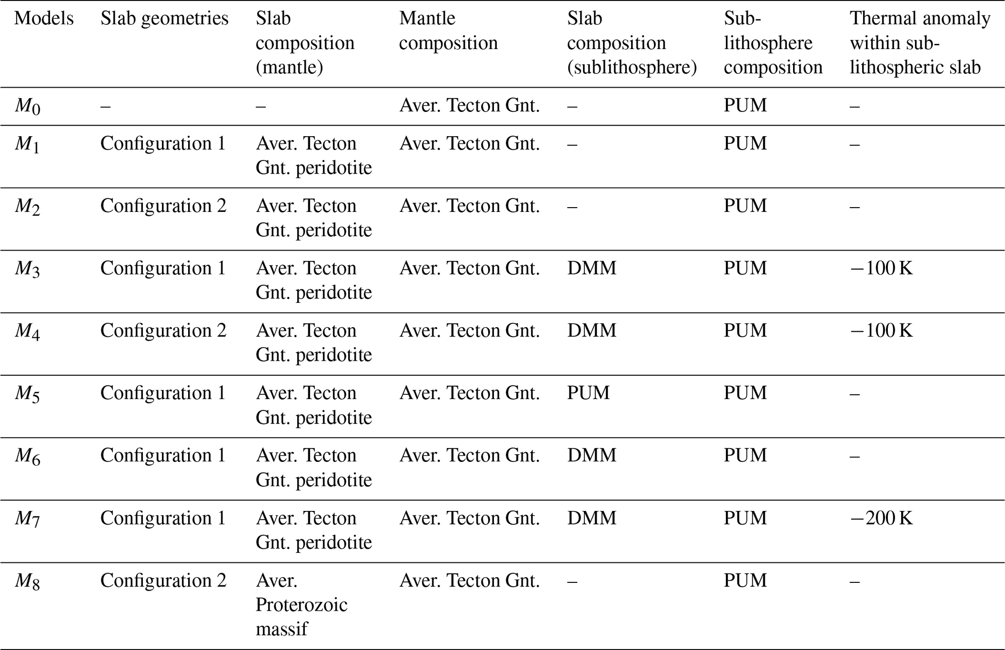
A positive density contrast between subducting material and the surrounding mantle material results in a negative buoyancy force. A density contrast is introduced into the LitMod model by a difference in composition between the subducting denser slab and the surrounding mantle (Fig. 9). Here, we use Tecton-like compositions for the lithosphere and the subducting slab segments since the Alpine slab segments result from continent–continent collision (Tables 1 and 2). A later model features a Proterozoic slab composition (M8). Depleted mid-oceanic ridge basalt mantle (DMM) and primitive upper mantle (PUM) are used for the sublithospheric domain. In addition to the density contrast within the sublithosphere, a temperature anomaly of −100 K is introduced for the sublithospheric part. Later models include a variation of temperature anomalies (M5, M6, M7). Note those compositions are used as a first-order test and serve as a starting point for synthetic slab models to illustrate the compositional and thermal effect on the gravity signal by influencing the density distribution. They do not necessarily represent the compositional mantle environment in the Alpine region.
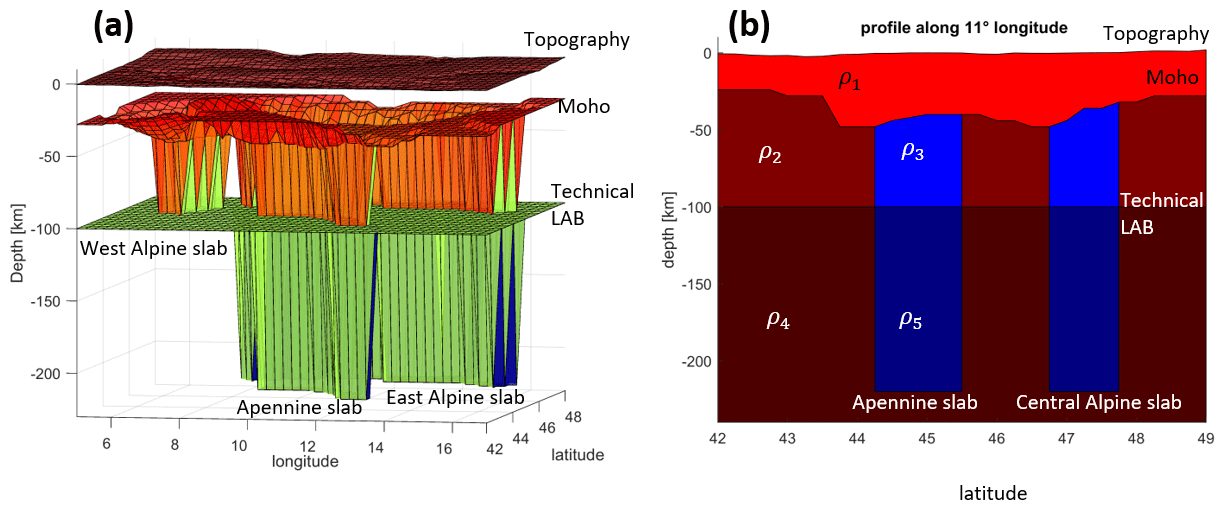
Figure 8(a) 3-D model set up using LitMod3D. Topography, Moho and LAB depth as well as the vertical incorporated slab models are used as input layers with assigned petrophysical and thermal properties. (b) Profile along 11∘ longitude through a LitMod model containing topography, crustal and lithospheric thickness as well as a slab segment. ρ1−5 indicate petrophysical and thermal property variations for each layer.
Results
The gravity signal of the predefined slab segments is forward calculated as well as the background model without incorporation of slab segments. The residual between both forward calculations gives the gravitational contribution of the slab segments, while other gravitational effects, like the topography or crustal thickness variation and mantle variations outside the slab, are not considered.
A slab segment with an average Tecton Gnt. composition (M1, M2) results in a slightly denser material compared to the surrounding mantle (M0), while a slab segment with a Proterozoic composition (M8) shows a less dense lithospheric structure compared to the reference model (M0); this composition results in less dense slab segment, which would not be subducted due to the positive buoyancy (Fig. 10). However, we aim to illustrate the effect composition has on the density distribution within the slab and to the surrounding mantle and show the importance of correct compositional information; therefore, we focus on the difference in density contrast between slab and surrounding mantle and neglecting the sign of the density contrast.

Figure 9(a) Density profile at 11∘ longitude and 45∘ latitude for the full vertical model space of 400 km depth. Density profiles for three different models (M0, M1, M9) with different compositional properties are shown. (b) Zoomed-in profile at the depth range of present slab segments.
The difference in density distribution (density contrast) within the slab segments with a Tecton composition (M1, M3) to the reference model (M0) is on the order of 5 kg m−3 for the lithosphere and on the order of 10 kg m−3 for the sublithospheric domain (Fig. 10a). The density variations within the lithospheric and sublithospheric slab domain are less than 1 kg m−3 resulting from both depth-dependent variations in pressure and temperature. Between lithosphere and sublithosphere, a rapid increase in density contrast is observed (Fig. 10a). The density contrast of a lithospheric Proterozoic slab composition (M9) to the reference model (M0) is on the order of −30 kg m−3 (Fig. 10b).

Figure 10(a) Residual density contrast for lithospheric and sublithospheric slab segments of model (M3) with Tecton-like composition within the lithosphere and PUM and DMM composition in the sublithosphere with an additional thermal anomaly of −100 K for the sublithospheric slab segment to the background model (M0). (b) Residual lithospheric density contrast of a Proterozoic lithospheric slab segment (M8) to a Tecton compositional surrounding mantle (M0). Residual density contrast is limited to the technical LAB as the sublithospheric part is identical to the reference model (see also Fig. 9b).
The gravity signal caused by the proposed slab segment configurations is estimated for lithosphere and sublithosphere separately. The forward-calculated gravity effect, at topographic surface level, for the slab Configuration 1 for the lithospheric part is on the order of 4 mGal, while the sublithospheric gravity signal is in the range of 7 mGal (Fig. 12a, b). The combined gravity signal is on the order of 12 mGal (Fig. 12c). The gravity signal in the Eastern Alps for Configuration 2 is significantly larger on the order of 17 mGal for the combined model (Fig. 12f).
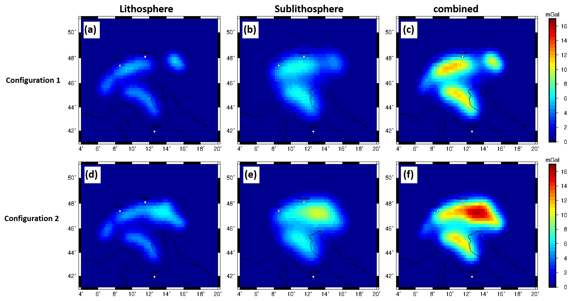
Figure 11Residual of the forward-calculated gz gravity signal of lithospheric slabs at surface station height based on LitMod models with Tecton-like compositions in the lithosphere and PUM and DMM compositions in the sublithosphere (M1, M2, M3, M4) with an additional thermal anomaly of −100 K for the sublithospheric slab segment, for predefined slab configurations to the background model (M0). (a–c) Configuration 1. (d–f) Configuration 2. Crustal and topographic contribution are nullified.
The calculated gravitational effect of a slab segment with Proterozoic composition and a Tecton surrounding mantle composition is on the order of −40 mGal for the gz component (Fig. 12a).
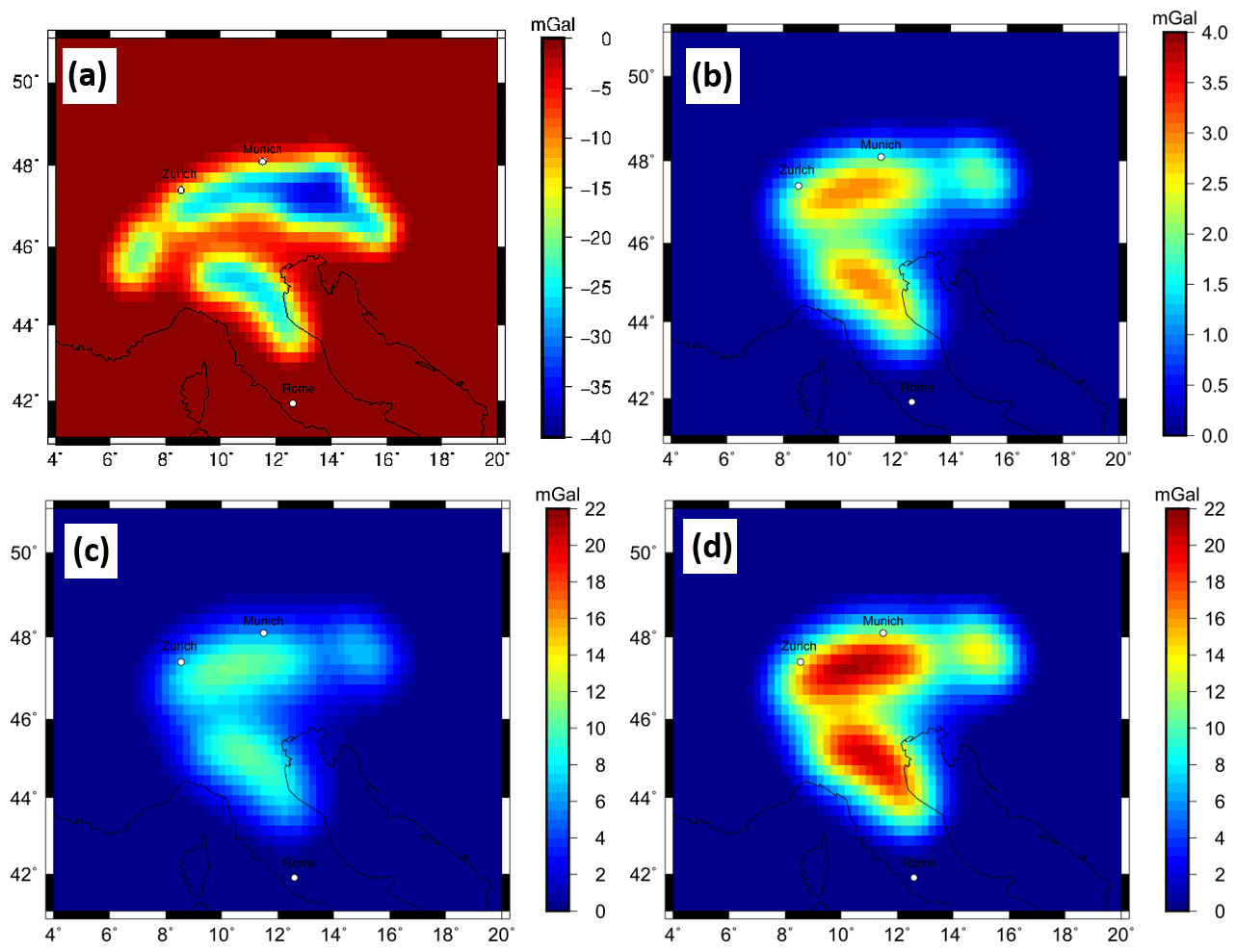
Figure 12(a) Forward-calculated gravity effect of a Proterozoic lithospheric slab segment to a Tecton compositional surrounding mantle for Configuration 2, obtained by calculating the residual between M8 and M0. (b) Gravity signal produced by purely compositional effect in the sublithosphere between a PUM and DMM composition, obtained by calculating the residual between M5 and M6. (c) Gravity signal produced by purely thermal anomaly of −100 K for a sublithospheric slab segment, obtained by calculating the residual between M3 and M6. (d) Gravity signal produced by purely thermal anomaly of −200 K for a sublithospheric slab segment obtained by calculating the residual between M6 and M7.
The gravity response to a compositional variation within the sublithosphere between the incorporated slab segment (DMM composition) and the surrounding mantle (PUM composition) is on the order of 4 mGal (Fig. 12b). The gravity response for a pure thermal anomaly of −100 K within the sublithospheric slab segment is on the order of 16 mGal (Fig. 12c), while a pure thermal anomaly of −200 K within the sublithospheric slab segment is on the order of 21 mGal.
The imprint of the gravity response caused by the density distribution based on direct conversion of seismic velocities (approach 1) is visible; however, individual and independent slab segments cannot be identified (Fig. 4). The strength of this approach is that it is fast to implement and can provide a first-order characterization of the gravity signal and slab geometries of subducting lithosphere. However, a clear characterization of subducting slab segments is not possible. First of all, the density model depends on the resolution and regularization of the seismological model, which can lead to distortions in the gravity response (e.g. Root, 2020). The method is dependent on the choice of the conversion factor and might overestimate the density (see the large negative anomaly in the Ligurian Sea). The conversion factor is a strong simplification of nature and for such a geodynamic complex area, a constant conversion factor is not adequate.
The forward-calculated gravity field with competing predefined slab geometries (approach 2) shows a clear gravity signal, where the individual slab segments are distinguishable (Fig. 6).
A relative gravity low related to the slab gap in the Eastern Alps is a prominent feature in the gravity signal of Configuration 1 (Fig. 6a). The Eastern Alpine slab segment of Configuration 1, due to its relatively small volume, results in a lower signal compared to the Central Alpine slab segment.
Configuration 2 shows a larger gravity signal in the Eastern Alps up to 100 mGal (Fig. 6b) compared to Configuration 1. The increase of the gravity signal is attributed to the subduction of both Eurasian and Adriatic lithosphere in the Eastern Alps. The gravity signal shows a continuous transition from the Central Alps to the Eastern Alps, where the contribution of the destined slab segment cannot be distinguished in the resulting gravity field (Fig. 6b). In the Western Alps, Configurations 1 and 2 show a lower gravity signal compared to the Central Alps. This is attributed to the much shallower Western Alpine slab segment that penetrates down to 100 km depth.
The gravity signal is influenced by both the assigned density contrast and thickness of the slab. A trade-off between both parameters is clearly observable, as the same gravity response of the slab configuration can be achieved with different values of density contrast and slab thickness, therefore making it impossible to derive slab properties in the form of density contrast and slab thickness from the gravity field (Fig. 7).
The calculated densities in LitMod3D models (approach 3) are estimated by taking temperature and pressure variations into account based on an assigned composition. The composition has a strong influence on the resulting density contrast. In the case that the compositional contrast between slab segment and surrounding mantle is small, the density contrast is consequently small as well (Figs. 9 and 10a). With increasing compositional differences, the density contrast increases as well. A strong density contrast within the slab segment is recognizable between lithospheric and sublithospheric domains (Fig. 10a and b), while the variations between the slab and surrounding mantle remain small.
The gravity signal in the Eastern Alps shows a significantly larger signal from the lithosphere and sublithosphere domains for Configuration 2 (Fig. 11d–f) compared to Configuration 1 (Fig. 11a–c). The different slab segments are distinguishable with the exception of the two slab segments in the Eastern Alps in Configuration 2 (Fig. 11). The contribution from the lithospheric domain to the gravity signal is smaller than that from the sublithospheric domain (Fig. 11b and e). However, the slab gap and the eastern slab segment feature can be recognized in the lithospheric part in Configuration 1 but not in the gravity signal of the full model.
The Proterozoic slab segment has a larger gravity response compared to the Tecton-like composition. This gravitational signal is negative due to the less dense Proterozoic composition in comparison to the reference model (M0) (Fig. 12a).
Sublithospheric composition has only a small influence on the gravity field, on the order of 4 mGal (Fig. 12b). However, a thermal anomaly within the sublithospheric slab on the order of −100 K results in a gravitational response of 16 mGal (Fig. 12c) and for a −200 K anomaly on the order of 21 mGal (Fig. 12d). Both the composition and the thermal variation influence the density and consequently the gravity response. However, the thermal component is a much larger contributor.
For the three approaches (Sects. 3, 4.1 and 4.2), a measurable gravity effect of the subducting slab segments is observable. The independent slab segments are distinguishable to a certain degree with the exception of the bivergent slab configuration in the Eastern Alps (Figs. 6, 11) and the model containing converted density from seismic velocities (Fig. 4), while the slab configurations cannot be separated at satellite altitude (see the Appendix). Forward-calculated gravity anomalies from converted density distribution suggest a gravitational signal of the slab segments on the order of 40 mGal, which corresponds to a density contrast of 20 to 40 kg m−3 in the models with predefined slab geometry. The models with a Tecton-like composition suggest a gravity effect of the slab segments on the order of only 16 mGal, corresponding to a density contrast of 20 kg m−3 in the simple model. Increasing the compositional difference with a Tecton composition suggests a gravity signal on the order of 30 mGal and is in line with the converted density model.
All three methods show a positive gravity signal contribution, which can be related to subcrustal density variations for approach 1 and to predefined subcrustal slab segments for approaches 2 and 3, up to 40 mGal to the Alpine gravity field. That is significant in comparison to the observed Bouguer anomaly with a minimum of ∼ −200 mGal. If this contribution is not considered, a significant part of the gravity signal is attributed to crustal thickness or intracrustal sources. Due to the long-wavelength appearance of the gravity effect which might not be relevant for small-scale or local studies, the effect is only seen as a shift. For gravity models of larger areas (e.g. Eastern Alps) or even entire regions, this should not be neglected. For one, estimates of crustal thickness or the mass distribution are significantly biased, and placing the Alps in the geodynamic context of the surroundings requires a careful and complete consideration of all sources in order to provide the realistic density distribution required for geodynamic models (e.g. Reuber et al., 2019).
We have addressed the potential gravity effect of proposed slab segments in the Alpine region using three different modelling approaches.
One approach is converted density from seismic tomography. In the resulting gravity signal, the imprint of slab segments is visible; however, distinguishing between the different and independent slab segments is not possible.
Models with predefined slab segments are dependent on the assigned density contrast and volume as well as on the predefined positions of the slab segments. The gravity signal caused by the slab segments is sharp and can be separated for the different slab segments for the gravity field at the surface. Significant gravity contributions to the Alpine gravity from slab segments below 200–250 km are unlikely.
Another approach involves combining petrophysical–geophysical modelling results in the most complex models. The calculated density variation within the slab is rather small compared to the density contrast between lithosphere and sublithosphere. The density distribution within the slabs, and consequently the gravity field, is highly influenced by the slab composition and thermal structure.
Subcrustal density variation (approach 1) and predefined slab segments (approaches 2 and 3) suggest a positive subcrustal gravity contribution of up to 40 mGal. Even though this might be considered as a maximum gravity estimation of slabs, this value is significant, even compared to the observed Bouguer anomaly low of −200 mGal along the Alps. The interpretation of density variation in the mantle in terms of subducting slab structures is a means to provide a meaningful representation of the geodynamic complex Alpine area. For future studies, correct slab density structure is crucial to provide a representation of the Alpine geodynamic setting. Precise estimations of the slab density structure require a correct crustal density and crustal thickness model. With the integration of further observables, it might be possible to judge the correct slab configuration beneath the Alps. Furthermore, future studies based on the AlpArray network will be of high interest in better defining slab geometries as well as their properties.
For all Alpine density models presented above (Sects. 3, 4.1 and 4.2), we have also calculated gravity gradients at a station height of 225 km. This station height corresponds to the second mission phase of GOCE carried out by ESA.
We anticipated that gravity gradients measured by the GOCE satellite mission are sensitive to the slab segments in the Alpine region. Our result show that the long wavelength signal of the different present slab segments contributes to a large-scale gravity response where the different contributors cannot be separated. Therefore, we conclude that against our anticipation gravity gradients at satellite height are in fact not sensitive to the Alpine slab configuration. We show the gravity gradients here (mainly the gzz component) for completeness.
Measured gravity gradients from the GOCE mission (Bouman et al., 2016), which were corrected for topography and bathymetry, range from 2.5 to −2.5 E at a satellite altitude of 225 km (Fig. A1). A negative gravity anomaly of −2.5 E in the gzz component is observed equivalent to the vertical gz component (Fig. A2). However, no clear sign for subducting lithosphere can be observed in any component of the gravity gradient tensor.
The forward-calculated gzz component at 225 km station height from a density model (Sect. 3) with converted densities ranges from −3.5 to 0.7 E (Fig. A2). A positive gravity signal of about 0.5 E in the Apennine and Alpine regions is observed, which could be linked to subducting slab segments. However, it is impossible to separate specific slab segments.
Forward-calculated Tesseroid models (Sect. 4.1) for slab Configurations 1 and 2 with a constant density contrast of 60 kg m−3 and a constant thickness of 80 km result in a less sharp gravity signal for the gzz component at a station height of 225 km (Fig. A3) compared to the gz component at station height of 6040 m (Fig. 6). The gravity signal for the gzz component is in the range of 0.8 to 1 E. At satellite altitude, the gravity signal is observed as a large area with a positive gravity effect for Configurations 1 and 2. The contribution of the different slab segments to this positive gravity effect is not distinguishable. The only recognizable difference is the size of this positive gravity signal. Configuration 1 shows a smaller anomaly due to a lower volume of subducting material in the Eastern Alps.
In addition, the signal strength for the forward-calculated gzz component shows the same dependency of signal strength to the density contrast and slab thickness (Fig. A4) as the gz component (Fig. 7). The signal strength of the gzz component ranges for the 12 different combinations from 0.3 to 2 E (Fig. A4). The gravity signal cannot be separated and affiliated with a certain slab segment. The gzz gradient signal shows a large blurry gravity high over the Alps, which thins out to the edges.
The gravity effect for the LitMod models (Sect. 4.2) with the slab Configuration 1 shows in the lithosphere domain a signal strength of about 0.05 E, while the sublithospheric gravity signal is in the range of 0.1 E for the gzz component at a satellite altitude of 225 km. The combined gravity signal is on the order of 0.14 E (Fig. A5). A Proterozoic slab produces a larger amplitude in signal strength; however, the different slab segments cannot be separated again (Fig. A6).
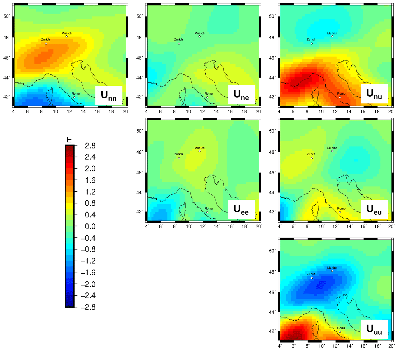
Figure A1GOCE gradients at 225 km after Bouman et al. (2016) corrected for topography and bathymetry with a 5∘ extension to remove far-field effects. The gravity gradients are presented in a north–east–up coordinate system.

Figure A2Forward-calculated gzz gravity signal from relative density distribution converted from relative seismic velocities using a conversion factor of 0.3 for the 225 km station height.
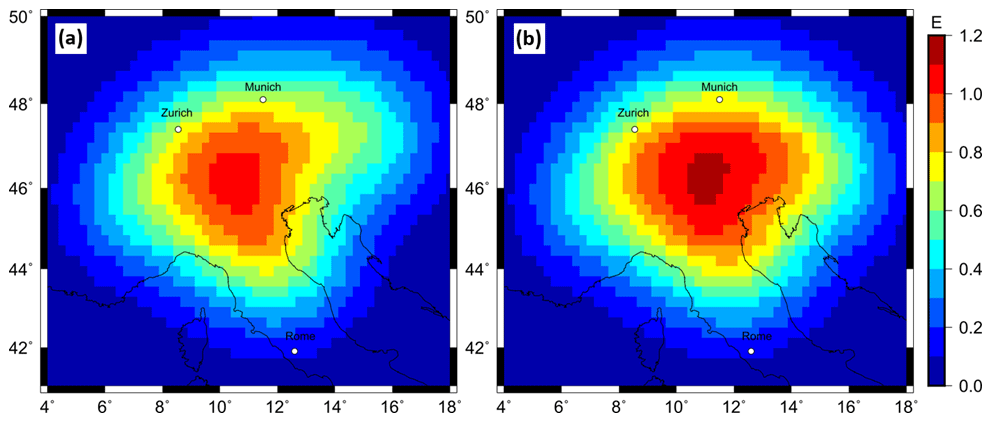
Figure A3Forward-calculated gzz gravity signal at a station height of 225 km from predefined subcrustal slab geometries with a content density contrast of 60 kg m−3 and a constant thickness of 80 km. (a) Slab configuration of Configuration 1. (b) Slab configuration of Configuration 2.
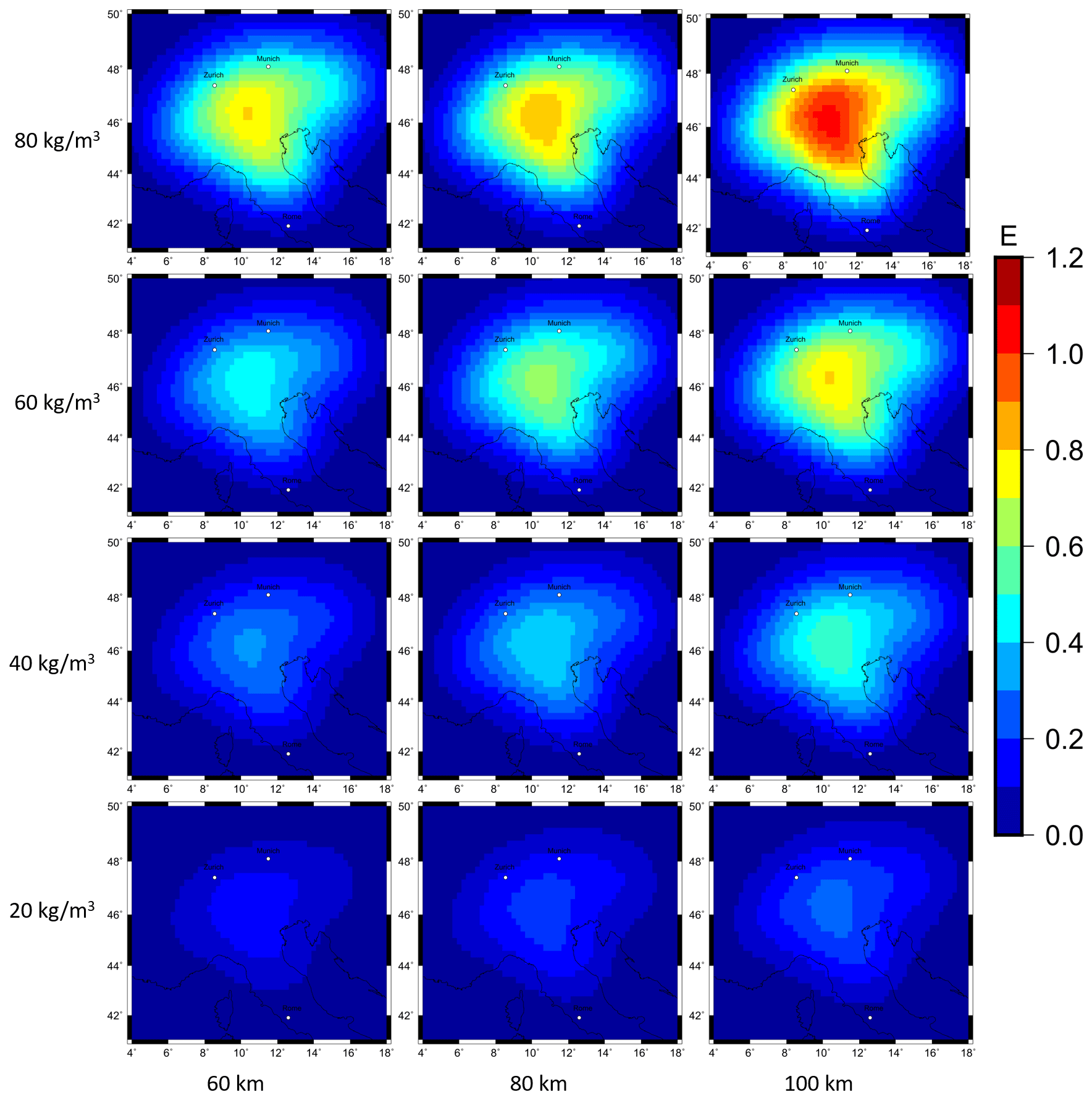
Figure A4Forward-calculated gzz gravity signal for 12 different combinations of density contrast and slab thickness at a station height of 225 km for subcrustal slab Configuration 1.
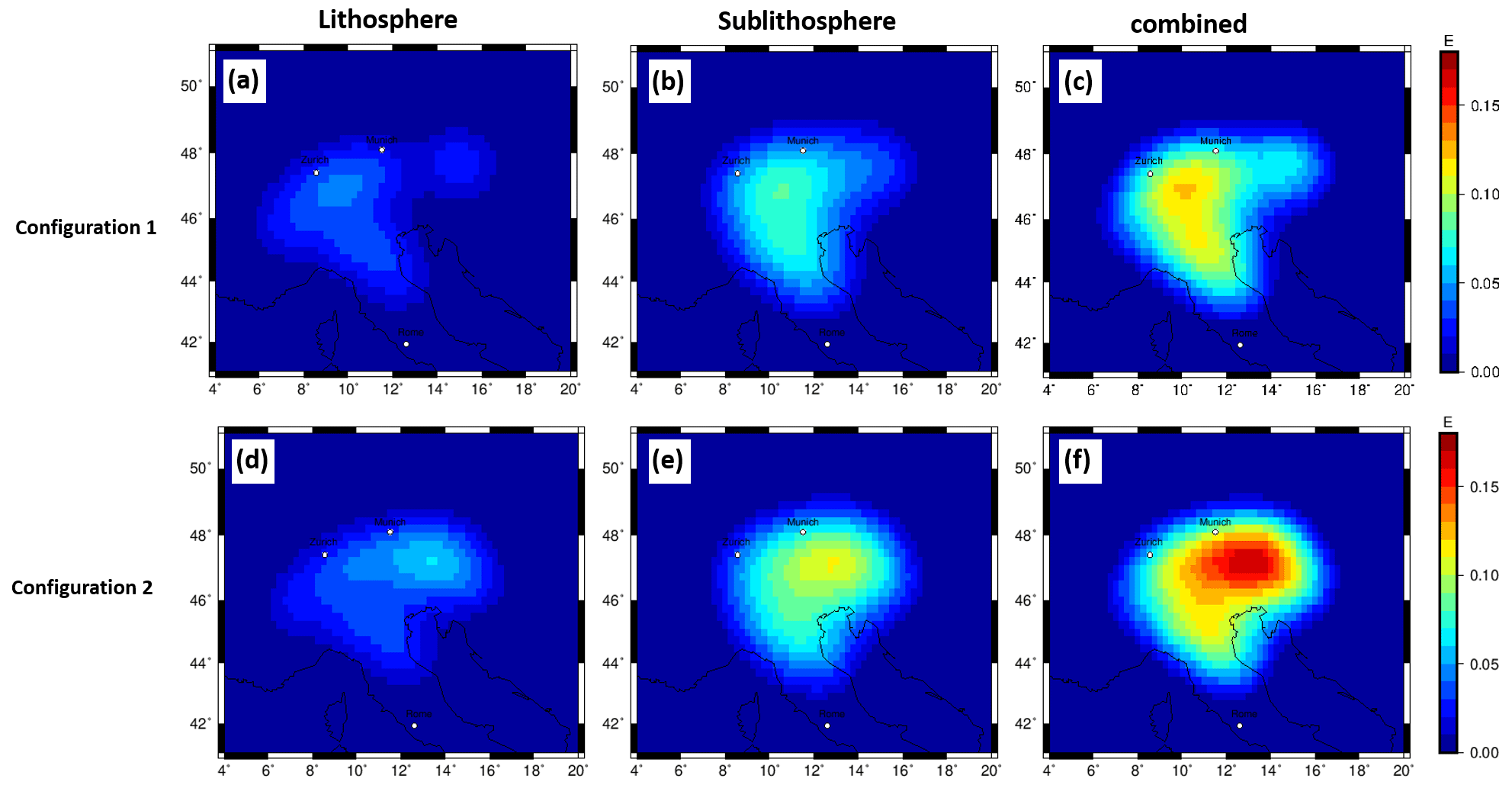
Figure A5Forward-calculated gzz gravity signal at satellite altitude of 225 km based on LitMod models with Tecton-like compositions in the lithosphere and PUM and DMM compositions in the sublithosphere (M1, M2, M3, M4) with an additional thermal anomaly of −100 K for the sublithospheric slab segment, for predefined slab configuration to the background model M0. (a–c) Configuration 1. (d–f) Configuration 2. Topographic and crustal effects are nullified.
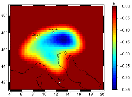
Figure A6Forward-calculated gravity effect for the gzz component at satellite height of a Proterozoic lithospheric slab segment to a Tecton compositional surrounding mantle for Configuration 2 obtained by calculating the residual between M8 and M0.
Tesseroids is available at https://tesseroids.readthedocs.io/en/stable/ (Uieda et al., 2016). LitMod3D is available at https://github.com/javfurchu/litmod (Fullea et al., 2009). The generic mapping tools (GMT) is available at https://github.com/GenericMappingTools/gmt/releases/tag/5.4.5 (Wessel and Luis, 2013).
The forward-calculated gravity signal models are publicly available through https://nextcloud.ifg.uni-kiel.de/index.php/s/BeRgpioKgAMkZbE, last access: 8 March 2021. ETOPO1 is available from the National Centers for Environmental Information (https://www.ngdc.noaa.gov/mgg/global/, Amante and Eakins, 2009). XGM2019 is available through the International Centre for Global Earth Models (http://icgem.gfz-potsdam.de/tom_longtime, Zingerle et al., 2020). MeRE2020 is available from the website of the IRIS Earth models repository (EMC; https://ds.iris.edu/ds/products/emc-mere2020/, El-Sharkawy et al., 2020). European Moho map can be accessed from https://www.seismo.helsinki.fi/mohomap/ (Grad et al., 2009). GOCE gravity gradients are available from https://earth.esa.int/eogateway/catalog/goce-global-gravity-field-models-and-grids (Bouman et al., 2016).
ML carried out the gravity modelling, visualized and interpreted the results and prepared the first manuscript draft. JE supervised the gravity modelling and interpretation, designed the original research project and handled acquisition of the financial support for the project leading to this publication and was responsible for writing (reviewing and editing). TM defined the slab configurations based on tectonic and seismological knowledge and was responsible for writing (reviewing and editing). AES created and provided the surface wave tomography model MeRE2020 and was responsible for writing (reviewing and editing).
The authors declare that they have no conflict of interest.
This article is part of the special issue “New insights on the tectonic evolution of the Alps and the adjacent orogens”. It is not associated with a conference.
The authors thank the reviewers, Carla Braitenberg and an anonymous referee, for their valuable suggestions, which helped to improve the manuscript significantly.
This study is part of the projects “Integrierte 3D Modellierung des Schwere- und Temperaturfelds zum Verständnis von Rheologie und Deformation der Alpen und ihrer Vorlandbecken – INTEGRATE” and “Surface Wavefield Tomography of the Alpine Region to Constrain Slab Geometries, Lithospheric Deformation and Asthenospheric Flow in the Alpine Region” funded by German Research Foundation (DFG) in the “Mountain Building Processes in Four Dimensions” SPP.
We thank the developers of open scientific software products which were utilized in this study: Tesseroids (Uieda et al., 2016), LitMod3D (Fullea et al., 2009; Afonso et al., 2008) and Generic Mapping Tools (GMT) (Wessel et al., 2013; Wessel and Luis, 2017).
This research has been supported by the Deutsche Forschungsgemeinschaft (grant nos. EB255/7-1 and EB 255/6-1).
This paper was edited by Giancarlo Molli and reviewed by Carla Braitenberg and one anonymous referee.
Afonso, J. C., Fernandez, M., Ranalli, G., Griffin, W. L., and Connolly, J. A. D.: Integrated geophysical-petrological modeling of the lithosphere and sublithospheric upper mantle: Methodology and applications, Geochem. Geophy. Geosy., 9, Q05008, https://doi.org/10.1029/2007GC001834, 2008.
Amante, C. and Eakins, B. W.: ETOP01 1 arc-minute global reliefmodel: Procedures, data sources and analysis, NOAA Tech. Memo., NESDIS NGDC-24, 19 pp., https://doi.org/10.7289/V5C8276M, 2009.
Artemieva, I. M.: Lithosphere structure in Europe from thermal isostasy, Earth-Sci. Rev., 188, 454–468, 2019.
Babuška, V., Plomerova, J., and Granet, M.: The deep lithosphere in the Alps: a model inferred from P residuals, Tectonophysics, 176, 137–165, 1990.
Beller, S., Monteiller, V., Operto, S., Nolet, G., Paul, A., and Zhao, L.: Lithospheric architecture of the South-Western Alps revealed by multiparameter teleseismic full-waveform inversion, Geophys. J. Int., 212, 1369–1388, 2018.
Bouman, J., Ebbing, J., Fuchs, M., Sebera, J., Lieb, V., Szwillus, W., Haagmans, R., and Novak, P.: Satellite gravity gradient grids for geophysics, https://earth.esa.int/eogateway/catalog/goce-global-gravity-field-models-and-grids (last access: 18 March 2021), Sci. Rep., 6, 1–11, 2016.
Braitenberg, C.: Exploration of tectonic structures with GOCE in Africa and across-continents, Int. J. Appl. Earth Obs., 35, 88–95, 2015.
Channell, J. E. T. and Horvath, F.: The African/Adriatic promontory as a palaeogeographical premise for Alpine orogeny and plate movements in the Carpatho-Balkan region, Tectonophysics, 35, 71–101, 1976.
Connolly, J. A. D.: The geodynamic equation of state: what and how, Geochem. Geophy. Geosy., 10, Q10014, https://doi.org/10.1029/2009GC002540, 2009.
Dewey, J. F., Helman, M. L., Knott, S. D., Turco, E., and Hutton, D. H. W.: Kinematics of the western Mediterranean, Geol. Soc. Spec. Publ., 45, 265–283, 1989.
Ebbing, J., Braitenberg, C., and Götze, H. J.: Forward and inverse modelling of gravity revealing insight into crustal structures of the Eastern Alps, Tectonophysics, 337, 191–208, 2001.
Ebbing, J., Braitenberg, C., and Götze, H. J.: The lithospheric density structure of the Eastern Alps, Tectonophysics, 414, 145–155, 2006.
El-Sharkawy, A., Meier, T., Lebedev, S., Behrmann, J., Hamada, M., Cristiano, L., Weidle, C., and Köhn, D.: The Slab Puzzle of the Alpine-Mediterranean Region: Insights from a new, High-Resolution, Shear-Wave Velocity Model of the Upper Mantle, Geochem. Geophy. Geosy., 21, e2020GC008993, https://doi.org/10.1029/2020GC008993, 2020.
Fichtner, A., van Herwaarden, D. P., Afanasiev, M., Simutė, S., Krischer, L., Çubuk-Sabuncu, Y., Colli, E., Saygin, E., Villaseñor, A., Trampert, J., Cupillard, P., Bunge, H., and Igel, H.: The collaborative seismic earth model: Generation 1, Geophys. Res. Lett., 45, 4007–4016, 2018.
Frisch, W.: Tectonic progradation and plate tectonic evolution of the Alps, Tectonophysics, 60, 121–139, 1979.
Fullea, J., Afonso, J. C., Connolly, J. A. D., Fernandez, M., García-Castellanos, D., and Zeyen, H.: LitMod3D: An interactive 3-D software to model the thermal, compositional, density, seismological, and rheological structure of the lithosphere and sublithospheric upper mantle, Geochem. Geophy. Geosy., 10, Q08019, https://doi.org/10.1029/2009GC002391, 2009.
Fullea, J., Fernàndez, M., Afonso, J. C., Vergés, J., and Zeyen, H.: The structure and evolution of the lithosphere-asthenosphere boundary beneath the Atlantic-Mediterranean Transition Region, Lithos, 120, 74–95, 2010.
Ganguly, J., Freed, A. M., and Saxena, S. K.: Density profiles of oceanic slabs and surrounding mantle: Integrated thermodynamic and thermal modeling, and implications for the fate of slabs at the 660km discontinuity, Phys. Earth Planet. Inter., 172, 257–267, 2009.
Götze, H. J. and Krause, S.: The Central Andean gravity high, a relic of an old subduction complex?. J. S. Am. Earth Sci., 14, 799–811, 2002.
Götze, H. J. and Pail, R.: Insights from recent gravity satellite missions in the density structure of continental margins – With focus on the passive margins of the South Atlantic., Gondwana Res., 53, 285–308, 2018.
Götze, H. J., Lahmeyer, B., Schmidt, S., and Strunk, S.: The lithospheric structure of the Central Andes (20–26 S) as inferred from interpretation of regional gravity, in: Tectonics of the southern Central Andes, edited by: Reutter, K.-J., Scheuber, E., and Wigger, P. J., Springer, Berlin and Heidelberg, Germany, 7–21, 1994.
Grad, M., Tiira, T., and ESC Working Group: The Moho depth map of the European Plate, https://www.seismo.helsinki.fi/mohomap/ (last access: 18 March 2021) Geophys. J. Int., 176, 279–292, 2009.
Griffin, W. L., O'Reilly, S. Y., Ryan, C. G.: The composition and origin of sub-continental lithospheric mantle, in: MantlePetrology: Field Observations and High-Pressure Experimentation: A Tribute toFrancis R. (Joe) Boyd, edited by: Fei, Y., Berkta, C. M., and Mysen, B. O, Special Publication Geochemical Society, 6, 13–45, 1999.
Gutknecht, B. D., Götze, H. J., Jahr, T., Jentzsch, G., and Mahatsente, R.: Structure and state of stress of the Chilean subduction zone from terrestrial and satellite-derived gravity and gravity gradient data, Surv. Geophys., 35, 1417–1440, 2014.
Handy, M. R., Schmid, S. M., Bousquet, R., Kissling, E., and Bernoulli, D.: Reconciling plate-tectonic reconstructions of Alpine Tethys with the geological-geophysical record of spreading and subduction in the Alps, Earth-Sci. Rev., 102, 121–158, 2010.
Handy, M. R., Ustaszewski, K., and Kissling, E.: Reconstructing the Alps-Carpathians-Dinarides as a key to understanding switches in subduction polarity, slab gaps and surface motion, Int. J. Earth Sci., 104, 1–26, 2015.
Hawkesworth, C. J., Waters, D. J., and Bickle, M. J.: Plate tectonics in the Eastern Alps, Earth Planet. Sci. Lett., 24, 405–413, 1975.
Hetényi, G., Plomerová, J., Bianchi, I., Exnerová, H. K., Bokelmann, G., Handy, M. R., Babuška, V., and AlpArray-EASI Working Group: From mountain summits to roots: Crustal structure of the Eastern Alps and Bohemian Massif along longitude 13.3 E, Tectonophysics, 744, 239–255, 2018.
Holzrichter, N. and Ebbing, J.: A regional background model for the Arabian Peninsula from modeling satellite gravity gradients and their invariants, Tectonophysics, 692, 86–94, 2016.
Hua, Y., Zhao, D., and Xu, Y.: P wave anisotropic tomography of the Alps, J. Geophys. Res.-Sol. Ea., 122, 4509–4528, 2017.
Isaak, D. G.: High-temperature elasticity of iron-bearing olivines, J. Geophys. Res.-Sol. Ea., 97, 1871–1885, 1992.
Isaak, D. G., Anderson, O. L., Goto, T., and Suzuki, I.: Elasticity of single-crystal forsterite measured to 1700 K, J. Geophys. Res.-Sol. Ea., 94, 5895–5906, 1989.
Karato, S. I.: Importance of anelasticity in the interpretation of seismic tomography, Geophys. Res. Lett., 20, 1623–1626, 1993.
Karousová, H., Plomerová, J., and Babuška, V.: Upper-mantle structure beneath the southern Bohemian Massif and its surroundings imaged by high-resolution tomography, Geophys. J. Int., 194, 1203–1215, 2013.
Kästle, E. D., El-Sharkawy, A., Boschi, L., Meier, T., Rosenberg, C., Bellahsen, N., Cristiano, L., and Weidle, C.: Surface wave tomography of the alps using ambient-noise and earthquake phase velocity measurements, J. Geophys. Res.-Sol. Ea., 123, 1770–1792, 2018.
Kästle, E. D., Rosenberg, C., Boschi, L., Bellahsen, N., Meier, T., and El-Sharkawy, A.: Slab break-offs in the Alpine subduction zone, Int. J. Earth Sci., 109, 587–603, https://doi.org/10.1007/s00531-020-01821-z, 2020.
Kincaid, C. and Olson, P.: An experimental study of subduction and slab migration, J. Geophys. Res.-Sol. Ea., 92, 13832–13840, 1987.
Kissling, E., Schmid, S. M., Lippitsch, R., Ansorge, J., and Fügenschuh, B.: Lithosphere structure and tectonic evolution of the Alpine arc: new evidence from high-resolution teleseismic tomography, Geol. Soc. Mem., 32, 129–145, 2006.
Kogan, M. G. and McNutt, M. K.: Gravity field over northern Eurasia and variations in the strength of the upper mantle, Science, 259, 473–479, 1993.
Koulakov, I., Kaban, M. K., Tesauro, M., and Cloetingh, S. A. P. L.: P-and S-velocity anomalies in the upper mantle beneath Europe from tomographic inversion of ISC data, Geophys. J. Int., 179, 345–366, 2009.
Le Breton, E., Handy, M. R., Molli, G., and Ustaszewski, K.: Post-20 Ma motion of the Adriatic Plate: New constraints from surrounding orogens and implications for crust-mantle decoupling, Tectonics, 36, 3135–3154, 2017.
Lippitsch, R., Kissling, E., and Ansorge, J.: Upper mantle structure beneath the Alpine orogen from high-resolution teleseismic tomography, J. Geophys. Res.-Sol. Ea., 108, B8, https://doi.org/10.1029/2002JB002016, 2003.
Lüschen, E., Lammerer, B., Gebrande, H., Millahn, K., Nicolich, R., and TRANSALP Working Group: Orogenic structure of the Eastern Alps, Europe, from TRANSALP deep seismic reflection profiling, Tectonophysics, 388, 85–102, 2004.
Lüschen, E., Borrini, D., Gebrande, H., Lammerer, B., Millahn, K., Neubauer, F., Nicolich, D., and TRANSALP Working Group: TRANSALP – deep crustal Vibroseis and explosive seismic profiling in the Eastern Alps, Tectonophysics, 414, 9–38, 2006.
Lyu, C., Pedersen, H. A., Paul, A., Zhao, L., and Solarino, S.: Shear wave velocities in the upper mantle of the Western Alps: new constraints using array analysis of seismic surface waves, Geophys. J. Int., 210, 321–331, 2017.
Mahatsente, R.: Plate Coupling Mechanism of the Central Andes Subduction: Insight from Gravity Model, J. Geodetic Sci., 9, 13–21, 2019.
McDonough, W. F. and Sun, S. S.: The composition of the Earth, Chem. Geol., 120, 223–253, 1995.
McKenzie, D. and Fairhead, D.: Estimates of the effective elastic thickness of the continental lithosphere from Bouguer and free air gravity anomalies, J. Geophys. Res.-Sol. Ea., 102, 27523–27552, 1997.
Mitterbauer, U., Behm, M., Brückl, E., Lippitsch, R., Guterch, A., Keller, G. R., Koslovskaya, E., Rumpfhuber, E., and Šumanovac, F.: Shape and origin of the East-Alpine slab constrained by the ALPASS teleseismic model, Tectonophysics, 510, 195–206, 2011.
Nocquet, J. M. and Calais, E.: Geodetic measurements of crustal deformation in the Western Mediterranean and Europe, Pure Appl. Geophys., 161, 661–681, 2004.
Piromallo, C., and Morelli, A.: P wave tomography of the mantle under the Alpine-Mediterranean area, J. Geophys. Res.-Sol. Ea., 108, B2, https://doi.org/10.1029/2002JB001757, 2003.
Reuber, G., Meier, T., Ebbing, J., El-Sharkawy, A., and Kaus, B.: Constraining the dynamics of the present-day Alps with 3D geodynamic inverse models-model version 0.2, Geophys. Res. Abs., 21, p. 1, 2019.
Root, B. C.: Comparing global tomography-derived and gravity-based upper mantle density models, Geophys. J. Int., 221, 1542–1554, 2020.
Schmid, S. M., Fügenschuh, B., Kissling, E., and Schuster, R.: Tectonic map and overall architecture of the Alpine orogen, Eclogae Geol. Helv., 97, 93–117, 2004.
Serpelloni, E., Vannucci, G., Anderlini, L., and Bennett, R. A.: Kinematics, seismotectonics and seismic potential of the eastern sector of the European Alps from GPS and seismic deformation data, Tectonophysics, 688, 157–181, 2016.
Spada, M., Bianchi, I., Kissling, E., Agostinetti, N. P., and Wiemer, S.: Combining controlled-source seismology and receiver function information to derive 3-D Moho topography for Italy, Geophys. J. Int., 194, 1050–1068, 2013.
Spakman, W., and Wortel, R.: A tomographic view on western Mediterranean geodynamics, in: The TRANSMED atlas, The Mediterranean region from crust to mantle, edited by: Cavazza, W., Roure, F., Spakman, W., Stampfli, G. M., and Ziegler, P. A., Springer, Berlin and Heidelberg, Germany, 31–52, 2004.
Spooner, C., Scheck-Wenderoth, M., Götze, H.-J., Ebbing, J., Hetényi, G., and the AlpArray Working Group: Density distribution across the Alpine lithosphere constrained by 3-D gravity modelling and relation to seismicity and deformation, Solid Earth, 10, 2073–2088, https://doi.org/10.5194/se-10-2073-2019, 2019.
Stampfli, G. M. and Borel, G. D.: A plate tectonic model for the Paleozoic and Mesozoic constrained by dynamic plate boundaries and restored synthetic oceanic isochrons, Earth Planet. Sci. Lett., 196, 17–33, 2002.
Tadiello, D. and Braitenberg, C.: Gravity modeling of the Alpine lithosphere affected by magmatism based on seismic tomography, Solid Earth, 12, 539–561, https://doi.org/10.5194/se-12-539-2021, 2021.
Tašárová, Z. A.: Towards understanding the lithospheric structure of the southern Chilean subduction zone (36∘ S–42∘ S) and its role in the gravity field, Geophys. J. Int., 170, 995–1014, 2007.
Tiberi, C., Diament, M., Lyon Caen, H., and King, T.: Moho topography beneath the Corinth Rift area (Greece) from inversion of gravity data, Geophys. J. Int., 145, 797–808, 2001.
Uieda, L., Barbosa, V. C., and Braitenberg, C.: tesseroids: Forward-modeling gravitational fields in spherical coordinates, Geophysics, 81, 41–48, 2016.
Vacher, P., Mocquet, A., and Sotin, C.: Computation of seismic profiles from mineral physics: the importance of the non-olivine components for explaining the 660km depth discontinuity, Phys. Earth Planet. In., 106, 275–298, 1998.
Vrabec, M. and Fodor, L.: Late Cenozoic tectonics of Slovenia: structural styles at the Northeastern corner of the Adriatic microplate, in: The Adria microplate: GPS geodesy, tectonics and hazards, edited by: Pinter, N., Grenerczy, G., Weber, J., Medak, D., and Stein, S., Springer, Dordrecht, The Netherlands, 151–168, 2006.
Wang, Y., He, Y., Lu, G., and Wen, L.: Seismic, thermal and compositional structures of the stagnant slab in the mantle transition zone beneath southeastern China, Tectonophysics, 775, 228208, https://doi.org/10.1016/j.tecto.2019.228208, 2020.
Webb, S. J.: The use of potential field and seismological data to analyze the structure of thelithosphere beneath southern Africa, PhD thesis, University of the Witwatersrand, Johannesburg, 377 pp., 2009.
Wessel, P. and Luis, J. F.: The GMT/MATLAB Toolbox, Geochem. Geophy. Geosy., 18, 811–823, 2017.
Wessel, P., Smith, W. H., Scharroo, R., Luis, J., and Wobbe, F.: Generic mapping tools: improved version released, Eos T. Am. Geophys. Un., 94, 409–410, 2013.
Workman, R. K. and Hart, S. R.: Major and trace element composition of the depleted MORB mantle (DMM), Earth Planet. Sci. Lett., 231, 53–72, 2005.
Zeyen, H. and Fernàndez, M.: Integrated lithospheric modeling combining thermal, gravity, and local isostasy analysis: Application to the NE Spanish Geotransect, J. Geophys. Res.-Sol. Ea., 99, 18089–18102, 1994.
Zhao, L., Paul, A., Malusà, M. G., Xu, X., Zheng, T., Solarino, S., Guillot, S., Schwartz, S., Dumont, T., Salimbeni, S., Aubert, C., Pondrelli, S., Wang, Q., and Zhu, R.: Continuity of the Alpine slab unraveled by high-resolution P wave tomography, J. Geophys. Res.-Sol. Ea., 121, 8720–8737, 2016.
Zingerle, P., Pail, R., Gruber, T., and Oikonomidou, X.: The combined global gravity field model XGM2019e, http://icgem.gfz-potsdam.de/tom_longtime (last access: 18 March 2021), J. Geodesy, 94, 1–12, 2020.
- Abstract
- Introduction
- Data
- Conversion of seismic velocities into density distribution
- Slab models
- Discussion
- Conclusions
- Appendix A: Gravity gradients at satellite height
- Code availability
- Data availability
- Author contributions
- Competing interests
- Special issue statement
- Acknowledgements
- Financial support
- Review statement
- References