the Creative Commons Attribution 4.0 License.
the Creative Commons Attribution 4.0 License.
 | 30 Mar 2021
The impact of seismic interpretation methods on the analysis of faults: a case study from the Snøhvit field, Barents Sea
Jennifer E. Cunningham
Nestor Cardozo
Chris Townsend
Richard H. T. Callow
Five seismic interpretation experiments were conducted on an area of interest containing a fault relay in the Snøhvit field, Barents Sea, Norway, to understand how the interpretation method impacts the analysis of fault and horizon morphologies, fault lengths, and throw. The resulting horizon and fault interpretations from the least and most successful interpretation methods were further analysed to understand their impact on geological modelling and hydrocarbon volume calculation. Generally, the least dense manual interpretation method of horizons (32 inlines and 32 crosslines; 32 ILs × 32 XLs, 400 m) and faults (32 ILs, 400 m) resulted in inaccurate fault and horizon interpretations and underdeveloped relay morphologies and throw, which are inadequate for any detailed geological analysis. The densest fault interpretations (4 ILs, 50 m) and 3D auto-tracked horizons (all ILs and XLs spaced 12.5 m) provided the most detailed interpretations, most developed relay and fault morphologies, and geologically realistic throw distributions. Sparse interpretation grids generate significant issues in the model itself, which make it geologically inaccurate and lead to misunderstanding of the structural evolution of the relay. Despite significant differences between the two models, the calculated in-place petroleum reserves are broadly similar in the least and most dense experiments. However, when considered at field scale, the differences in volumes that are generated by the contrasting interpretation methodologies clearly demonstrate the importance of applying accurate interpretation strategies.
- Article
(12865 KB) - Full-text XML
- BibTeX
- EndNote


An accurate understanding of faults in the subsurface is critical for many elements of the hydrocarbon exploration and production industry. For example, faults control sediment and reservoir depositional systems, act either as conduits or baffles to fluid flow, are often the defining elements of structural traps, and impact the design of exploration and production wells (e.g. Athmer et al., 2010; Athmer and Luthi, 2011; Botter et al., 2017; Fachri et al., 2013a; Knipe, 1997; Manzocchi et al., 2008a, 2010). Subsurface faults are commonly interpreted from either reflection seismic data or attributes of that data by creating fault sticks on vertical cross sections (e.g. inlines ILs or crosslines XLs), which are then used to generate fault surfaces (e.g. Yielding and Freeman, 2016). Fault displacement is analysed by studying the interaction between the displaced horizon reflectors and the fault surface (e.g. Dee et al., 2005; Freeman et al., 1990; Needham et al., 1996). Although this is a commonly used interpretation method, the impacts of changing interpretation density (i.e. IL or XL spacing), interpretation from vertical vs. horizontal sections, and the effects of manual (2D line-by-line auto-tracking) vs. 3D auto-tracking techniques have not been systematically investigated.
The interpretation of faults in seismic data has been the focus of many studies. Badley et al. (1990) were the first to publish a systematic approach to the seismic interpretation of faults using fault displacement analysis. Freeman et al. (1990) explained how fault displacement analysis can be used in the quality-control process of fault interpretation. The interpreted horizon–fault intersections and subsequent fault displacement profiles in seismic data have also been described as ellipsoidal in isolated, single faults. When faults are not isolated, displacement profiles exhibit more complex geometries (i.e. multiple maxima), which can help to determine the structural history of fault linkage (Needham et al., 1996). A complete workflow for 3D structural interpretation in seismic data using various attribute volumes, reflection data, rendered volumes, and an overview of structural framework building has been presented by Yielding and Freeman (2016). In addition, Solum et al. (2016) recommended a combination of seismic interpretation, the analysis of structure maps, fieldwork, and geomodelling as the fundamentals of structural analysis. Interpreted fault surfaces can be quality-controlled by projecting longitudinal and shear strain (vertical and horizontal components of dip separation gradient) onto fault planes and assigning realistic strain limits in order to identify interpretation errors (Freeman et al., 2010). The aforementioned strain measurements are applied to determine the strain relationships of interpreted faults, assuming the data occur within a reasonable strain limit and after the quality-control process is complete (Freeman et al., 2010).
Uncertainty in fault interpretation has also been readily analysed, and previous works have focused on how significant uncertainties and interpretation biases exist in 2D and 3D seismic interpretation (Bond, 2015; Bond et al., 2011, 2007; Schaaf and Bond, 2019), as well as the impact of the image quality of seismic data on uncertainty in seismic interpretation (Alcalde et al., 2017). Uncertainty pertaining to fault properties, and the effect fault properties have on fluid flow simulations have also been analysed (Manzocchi et al., 2008b; Miocic et al., 2019). The impact of interpretation variability on structural trap definition and the juxtaposition of hydrocarbon-bearing reservoirs, as well as the subsequent implications for exploration and volume calculations, were tested and prove the impact of seismic interpretation bias in structurally defined hydrocarbon systems (Richards et al., 2015).
Many techniques have extended basic fault interpretation methods to better understand the link between faults in seismic surfaces and their properties in the subsurface. Dee et al. (2005) studied the application of structural geological analysis to a number of common industry-based techniques and workflows (e.g. fault seal, fluid accumulation, migration, fault property modelling). Seismic attributes have been analysed to study fault architecture and investigate fault sealing potential (Dutzer et al., 2010). Long and Imber (2010, 2012) used interpreted seismic surfaces to measure regional dip changes in order to map fault deformation in both a normal fault array and a relay ramp. Studies such as these, combined with the increasing availability of high-resolution 3D seismic data, have driven seismic structural analysis towards more detailed and quantitative studies. Iacopini and Butler (2011) and Iacopini et al. (2012) generated a workflow combining seismic attribute visualization, opacity filtering, and frequency decomposition to characterize deep marine thrust faults. In a case study from the Snøhvit field, a linkage between unsupervised seismic fault facies and fault-related deformation was established, and seismic amplitude was analysed to understand how folding near faults might influence near-fault amplitudes (Cunningham et al., 2021).
Synthetic seismic modelling has shed important light on the impact of seismic frequency on fault imaging, the seismic amplitudes contained in and around faults, and their linkage to fault-related deformation and fault illumination (Botter et al., 2014, 2016a, b). A comparison of faults in the Snøhvit field with synthetic seismic modelling showed the importance of incidence angle, azimuthal separation, and frequency on fault imaging (Cunningham et al., 2021).
Fluid flow across faults through deformed bedding and the sealing properties of faults have long been important topics in the petroleum industry (e.g. Bretan et al., 2011; Caine et al., 1996; Cerveny et al., 2004; Davatzes and Aydin, 2005; Edmundson et al., 2019; Fachri et al., 2013a, b, 2016; Fisher and Knipe, 1998; Knipe, 1997, 1992; Yielding et al., 1997). In addition, reservoir modelling techniques have been used to simulate this process (Fachri et al., 2013a), and synthetic seismic modelling has been used to understand the impact of faulting and fluid flow on seismic images (Botter et al., 2017).
Fault interpretation in seismic data has formed the basis of many studies over the decades, but no single study has looked specifically into seismic interpretation methodologies. It would seem logical to assume that increased interpretation density will result in a higher-resolution output (i.e. fault and horizon interpretation), but at the expense of the increased time required to perform the interpretation. It has yet to be fully evaluated whether these more detailed interpretations justify this increased time and effort or whether the end results are comparable to much more efficient interpretation strategies. Similarly, auto-tracking algorithms would appear to offer a shortcut to high-resolution horizon and fault interpretations, but how do these algorithms compare to the results of detailed manual interpretations? We address the impact of interpretation strategy on the quality of the final products and whether it is possible to identify an optimum balance between interpretation density, time required to do the interpretation, and the accuracy of the end result.
Our study tests the effect of interpretation methods (faults and displaced horizons) on aspects of fault analysis, with the aim to provide geoscientists with better knowledge of seismic interpretation and analysis of faults, as well as an explanation of the implications of improper interpretation and best-practice interpretation methods. We designed five fault and horizon interpretation experiments, which were conducted on a seismic volume from the Snøhvit field, Barents Sea. The resulting surfaces from each experiment (faults and horizons) were run through a fault analysis workflow. Key aspects of the workflow include the analysis of fault length and morphology, fault displacement (throw; Badley et al., 1990; Freeman et al., 1990; Needham et al., 1996), juxtaposed lithology (Allan, 1989; Fisher and Knipe, 1998; Knipe, 1992, 1997), dip separation gradient (Freeman et al., 2010), geological modelling (e.g. Jolley et al., 2007; Turner, 2006), and the subsequent petroleum volume calculations.
The Snøhvit gas and condensate field is located in the centre of the Hammerfest Basin on the southwest margin of the Barents Sea (Fig. 1a, b: Linjordet and Olsen, 1992). The ENE–WSW-trending Hammerfest Basin is ∼ 150 km long by 70 km wide and is bound in the north, southeast, and west by the Loppa High, Finnmark Platform, and Tromsø Basin, respectively. Rifting in the basin initiated in the Late Carboniferous–early Permian and drove the formation of the NE–SE-trending basin-bounding faults (Gudlaugsson et al., 1998). A second phase of rifting in the Late Jurassic–Early Cretaceous reactivated the basin-bounding faults and caused the basin to undergo large amounts of subsidence on both the northern and southern margins (Doré, 1995; Linjordet and Olsen, 1992; Ostanin et al., 2012; Sund et al., 1984). Due to differential subsidence during this period, the Hammerfest Basin widened and deepened westward, allowing for the accumulation of thicker sediment packages in the west (Linjordet and Olsen, 1992). A dome at the basin's central axis and a subsequent east–west-trending fault system formed during basin extension in the Early Jurassic–Barremian (Sund et al., 1984). These east–west-trending faults define the structure of the Snøhvit field and divide the field into northern and southern petroleum provinces (Sund et al., 1984). The main petroleum system components of the Snøhvit field are located within the Upper Triassic–Jurassic strata (Fig. 1c; Linjordet and Olsen, 1992). The focus of this study is on two of the east–west-trending faults across the Snøhvit field (Fig. 1b, blue and red lines). These two faults dip to the north, offset the Jurassic strata, and form a relay ramp structure (Fig. 1d). The area was chosen because relays are structurally complex and require special attention in their interpretation. Relays are also important in petroleum systems as they can create sediment distribution pathways, enable or disable fault seal (as all faults can), act as fluid flow pathways, and be a part of trap definitions (Athmer et al., 2010; Athmer and Luthi, 2011; Botter et al., 2017; Fachri et al., 2013a; Fossen and Rotevatn, 2016; Gupta et al., 1999; Knipe, 1997; Peacock and Sanderson, 1994; Rotevatn et al., 2007).

Figure 1(a) Geologic setting of the Hammerfest Basin. The area in (b) is marked by a black box. Modified from NPD fact maps. (b) Snøhvit field area. The dashed yellow line shows the extent of seismic data, and the orange rectangle highlights the study area. Map modified from Ostanin et al. (2012). The blue background refers to the Jurassic Hammerfest Basin, while the red shapes identify the areal extent of Lower–Middle Jurassic gas fields. The western and eastern fault in the study area are coloured blue and red, respectively. (c) Generalized lithostratigraphic column of the Barents Sea highlighting the horizons of interest. Modified from Ostanin et al. (2012). (d) North–south seismic IL (3342) through the middle of the Snøhvit field (X-X′ in b), with interpreted horizons and faults. Interpreted horizons are as follows. A: top Kolje, B: top Fuglen, C: top Fruholmen (c, d).
Five interpretation experiments (Exps. 1–5) were designed to test the impact of different seismic interpretation methods on the analysis of faults (Fig. 2). Each of these experiments (Fig. 2a) was completed on a chosen 5 × 5 km area covering the relay ramp (orange rectangle in Fig. 1b), and a fault analysis workflow was applied to the interpreted seismic horizon and fault surfaces from each experiment (Fig. 2b). The fault analysis workflow (Fig. 2b) integrated a comparison of seismic interpretation results and analyses of fault length, throw, dip separation gradients (longitudinal and shear strain), juxtaposed lithology, geological modelling, and calculation of hydrocarbon volumes. While the individual components of the fault analysis workflow have been applied previously (e.g. Elliott et al., 2012; Fachri et al., 2013a; Long and Imber, 2010, 2012; Rippon, 1985; Townsend et al., 1998; Wilson et al., 2009, 2013), no earlier studies have considered the impact of the seismic interpretation strategy on the outcomes of the fault analysis workflow.
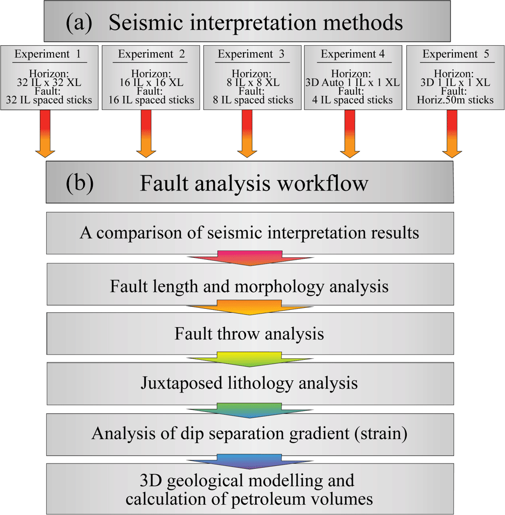
Figure 2The workflow used in this study. The fault analysis workflow (b) was completed in each of the seismic interpretation experiments (a).
The computer programmes Petrel™ and T7™ (formerly TrapTester™) were used in the seismic interpretation and fault analysis workflows, respectively. The seismic dataset used in this study was survey ST15M04, a merge of five 3D seismic streamer surveys that was provided by Equinor ASA and their partners (Petoro AS, Total E&P Norge AS, Neptune Energy Norge AS, and Wintershall Dea Norge AS) in the Snøhvit field. The ST15M04 volume was zero-phase pre-stack depth-migrated (PSDM; Kirchhoff), and both partial and full offset stacks were available. It was assumed that the velocity model used in the PSDM was correct and that the vertical scale of the processed volume (in depth) represents depth in metres. The inlines (ILs) and crosslines (XLs) are spaced at 12.5 m, and an increase in acoustic impedance is represented by a red peak (blue–red–blue). The interpretation was performed in depth to give the most representative view of the geological and structural relationships and to avoid re-stretching the data back into time. All five interpretation experiments were conducted on the near-stack data (5–20∘), as this dataset has been proven to give the most consistent fault imaging and best reflector continuity (i.e. Shuey, 1985). As the data are a merge of multiple datasets and vintages, the acquisition orientation geometries could not be considered although they are known to impact fault imaging (Cunningham et al., 2021).
3.1 Seismic interpretation
Two east–west-trending, north-dipping faults that form the relay ramp were interpreted (Fig. 1b, d). These two faults are termed the western and eastern faults (Fig. 1b and d, blue and red faults, respectively). Two faulted seismic reflectors (top Fuglen and Fruholmen formations; Fig. 1c–d) were also interpreted. These reflectors were chosen because the top Fuglen is a very strong, easily interpreted reflector, while the top Fruholmen is poorly imaged and is more challenging to interpret. Both the top Fuglen and top Fruholmen are peaks (increases in acoustic impedance). The Stø Formation, which falls between the Fuglen and Fruholmen tops, is a prolific petroleum reservoir. Five different seismic interpretation methods (Exps. 1–5) were used with the aim of systematically studying how seismic interpretation techniques (Fig. 2a) influence the fault analysis workflow (Fig. 2b). The first three experiments are manual 2D auto-tracking horizon interpretation techniques with different IL and XL spacing (from every 8 to 32 lines), while the fourth and fifth experiments are a combination of automated (3D auto-tracked horizons) and manual fault interpretations. In all experiments, the faults were interpreted first, followed by the horizons. 2D and 3D auto-tracking of all horizons used a seed confidence of 30 % and a basic 3 × 3 seed expansion value, which pushed the interpretation to the nearest eight seed points of the interpreted seed point on the peak. In 2D auto-tracking, seed expansion only occurs in 2D on the IL or XL being interpreted, while in 3D auto-tracking, the seed points extend in both the x and y directions from the interpreted seed point to the eight nearest seed locations. In both 2D and 3D, if a fault was encountered, the interpretation stopped and needed to be guided to the correct horizon on the other side of the fault. In all experiments, faults were interpreted as simple planar features in the seismic data. Although faults are complex 3D bodies in the subsurface, due to the seismic resolution of the data (i.e. Wood et al., 2015), this detail was not captured and has therefore not been considered further.
3.1.1 Exp. 1: 32 × 32
The top Fuglen and top Fruholmen reflectors were interpreted on every 32nd IL (north–south) and XL (east–west) using 2D auto-tracking (Fig. 3a, columns 1 and 2). Fault sticks were interpreted perpendicular to the average strike of the faults on every 32nd IL as largely planar features (Fig. 3a, column 3). The IL and XL spacing of interpretation in this experiment was equal to 400 m (every 32 ILs and XLs × 12.5 m IL and XL spacing).
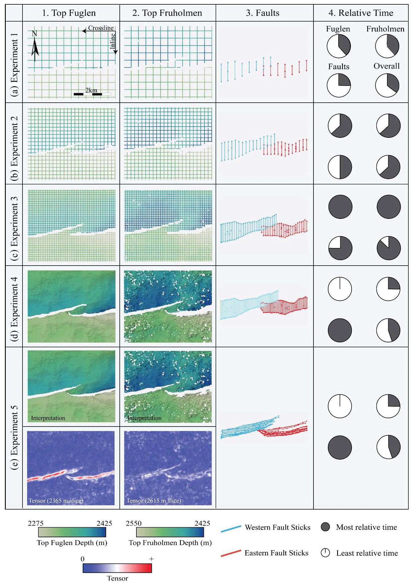
Figure 3Seismic interpretation methods for Exps. 1–5. (a) For Exp. 1 with 32 × 32 IL × XL spacing, fault sticks are interpreted on every 32nd IL. (b) For Exp. 2 with 16 × 16 IL × XL interpretation spacing, fault sticks are interpreted on every 16th IL. (c) For Exp. 3 with 8 × 8 IL × XL spacing, fault sticks are interpreted on every eighth IL. (d) For Exp. 4 with 3D auto-tracking (complete interpretation coverage of all ILs and XLs), fault sticks are interpreted on every fourth IL. (e) For Exp. 5 with 3D auto-tracking (columns 1 and 2, interpretation), faults are interpreted on depth slices of the tensor attribute at a spacing of 50 m (e.g. columns 1 and 2, tensor slices). Time estimations for the interpretation of the top Fuglen (column 1), top Fruholmen (column 2), the two faults (column 3), and the overall time taken for each experiment are displayed in column 4.
The interpretation of the two horizons and the two faults took the least amount of time when compared to all other experiments because of the large IL and XL spacing (Fig. 3a, column 4). Overall, this experiment was the quickest but sparsest interpretation method. Since the interpretation was manually conducted on an IL and XL basis, there was no quality control (QC) needed for the top Fuglen due to the high quality of this reflector. In particularly dim areas, 2D auto-tracking of the top Fruholmen required more manual input and some QC.
3.1.2 Exp. 2: 16 × 16
The two horizons were interpreted on every 16th IL and XL using 2D auto-tracking of the peaks for each reflector (Fig. 3b, columns 1 and 2). Fault sticks were interpreted on every 16th IL and are largely planar (Fig. 3b, column 3). The IL and XL spacing in this experiment was equal to an interpretation spacing of 200 m (every 16 ILs and XLs × 12.5 m).
The interpretation of both the horizons and faults in this experiment took twice the amount of time of Exp. 1, since the IL and XL spacing was halved. This experiment was ranked the second most time-consuming and the second sparsest overall (Fig. 3b, column 4). Since the interpretation in this experiment was manual, a similar level of QC was needed. There was high to lower confidence in the interpretation quality of the top Fuglen and top Fruholmen reflectors, as described in Exp. 1.
3.1.3 Exp. 3: 8 × 8
The two horizons were interpreted on every eighth IL and XL (Fig. 3c, columns 1 and 2). Fault sticks were interpreted on every eighth IL (Fig. 3c, column 3). The IL and XL spacing in this experiment is equal to an interpretation spacing of 100 m (every 8 IL and XL × 12.5 m).
The horizons and faults in this experiment took approximately 3 times longer to interpret than Exp. 1. This experiment was the densest of the manual interpretation methods (Exps. 1–3) and was therefore the most time-consuming (Fig. 3c, column 4). The quality control and interpretation confidence of the two reflectors is as described for Exps. 1 and 2.
3.1.4 Exp. 4: 3D tracked method with dip-parallel fault sticks
Horizons were tracked using the 3D auto-tracking algorithm in Petrel™, which resulted in complete interpretation coverage (all ILs and XLs interpreted) for the top Fuglen compared to almost complete coverage for the top Fruholmen (Fig. 3d, columns 1 and 2). Initially, we planned to apply a 3D automated fault interpretation method (Adaptive Fault Interpretation; Cader, 2018) for this experiment, but the algorithms currently available do not provide geologically realistic fault sticks that could be used in our workflow. As a result, fault sticks were interpreted on every fourth IL to capture the densest and most geologically realistic morphologies possible (Fig. 3d, column 3). The IL and XL spacings of horizon and fault interpretations in this experiment are 12.5 m (every IL and XL × 12.5 m spacing) and 50 m (every 4 ILs × 12.4 IL spacing), respectively. A 30 % seed confidence and a basic 3 × 3 seed point expansion were set in the auto-tracking of these surfaces.
The 3D auto-tracked interpretation of the top Fuglen was the fastest method as the reflector is well-imaged and therefore easily auto-tracked (Fig. 3d, column 1). The top Fruholmen was a little slower to run through the auto-track due to its poor seismic imaging (Fig. 3d, column 2). As a result, the top Fruholmen required more manual guidance for the auto-track to be successful, but it was still faster than all three manual interpretation methods (Exps. 1–3). The fault interpretation for this experiment was the most time-consuming as the spacing of fault sticks was the densest (Fig. 3d, column 3). Overall, Exp. 4 was tied for the second fastest to interpret (Fig. 3d, column 4), but it also contains the highest density of interpretation lines for both the horizons and faults. The QC of the top Fuglen was completely unnecessary in this small study area as the reflector was strong and easily auto-tracked. The QC of the top Fruholmen was more important since the reflector imaging is quite poor in some areas. The interpretation confidence for this case is high to moderately high for the top Fuglen and top Fruholmen, respectively.
3.1.5 Exp. 5: 3D auto-tracked horizons with horizontal (strike-parallel) fault sticks
This experiment used the same 3D auto-tracked horizons as discussed in Exp. 4 (Fig. 3e, columns 1 and 2, interpretation). However, faults were manually interpreted horizontally on depth slices spaced every 50 m using the tensor attribute to guide the interpretation (e.g. Fig. 3e, columns 1 and 2, tensor slices). The tensor attribute is generated using a symmetric and structurally oriented tensor, which detects the localized reflector orientation and is sensitive to changes in both the amplitude and continuity of the seismic reflectors (Bakker, 2002). This attribute was chosen as it is a well-known fault-enhancing attribute and is widely used in fault interpretation (e.g. Botter et al., 2016b; Cunningham et al., 2019). The resulting fault sticks (Fig. 3e, column 3) have a high degree of horizontal curvature as each stick traces a fault's entire lateral extent. Although the results have the same fault morphology as Exp. 4, the horizontal fault sticks look quite different than the planar dip-parallel fault sticks in all other experiments (Fig. 3, column 3).
The fault interpretation for this experiment was time-consuming as it required the generation of a tensor attribute prior to interpretation (Fig. 3e, column 4). Once the attribute was produced, the time to generate the fault interpretation was in the middle range of the time used for the other experiments. The interpretation confidence of the two reflectors is as described in Exp. 4.
3.1.6 A comparison of horizon and fault surface grids
The horizon interpretations and fault sticks were gridded into horizons and fault surfaces using the seismic 12.5 m grid spacing. The horizon surfaces were generated to stay true within ± 5 m of the interpretations for each of the five experiments, and no post-processing smoothing techniques were applied to the horizon gridding. Fault sticks in all five experiments were made into surfaces using a 50 m triangulated surface algorithm. This method was chosen as it generated a surface that was closest to the original fault stick interpretations. The fault and horizon surfaces were used as the input for the fault analysis workflow.
To understand the relative differences between the horizons from each experiment, thickness maps were generated between the most densely interpreted 3D auto-tracked horizons (Exps. 4 and 5) and the horizons generated from each of the manually based experiments (Exps. 1–3). Anywhere there is a good correlation between the auto-tracked and manual surfaces, there is very little or no thickness change, while in the case of a poor correlation, a greater range in thickness may result.
3.2 Fault length and morphology
Fault length (Fig. 4a) is defined as the maximum horizontal distance of a fault in three dimensions (Peacock et al., 2016; Walsh and Watterson, 1988). An analysis of fault length was conducted on the western and eastern faults (Fig. 1b, d) using the gridded fault surfaces. These data were extracted from the edge of the study area to the fault tipline for both faults. The data were graphically compared to understand the impact of the interpretation method on fault length.
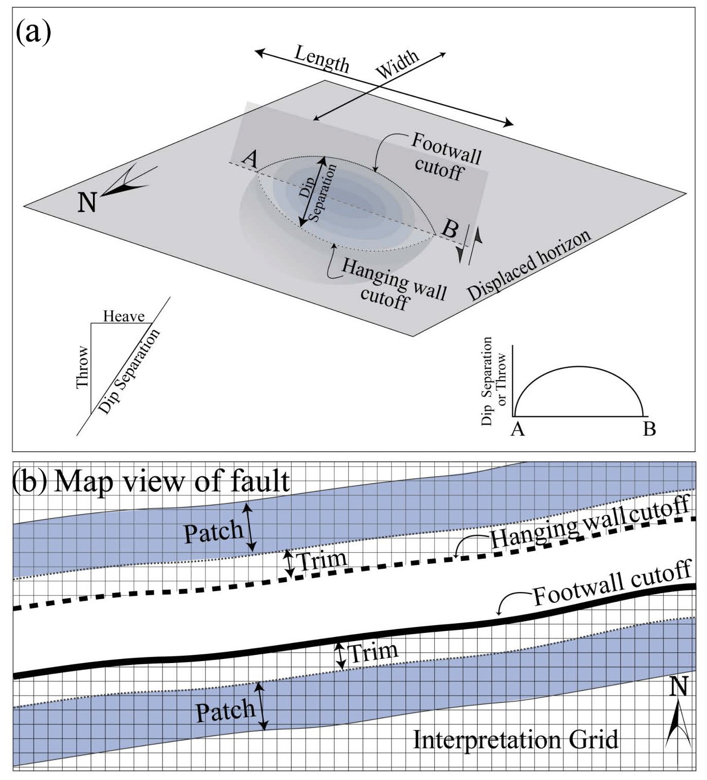
Figure 4Fault schematic and fault throw calculation method. (a) 3D diagram of an isolated normal fault showing the displacement field, hanging wall and footwall cutoff lines, fault length and width, dip separation, throw, and heave. (b) Map view of a fault with trim and patch distances used in the determination of hanging wall and footwall cutoff lines (Modified from Yielding and Freeman, 2016, p. 164). The patch and trim distances used in this analysis were 150 and 75 m, respectively. Concepts in this figure are based on findings from Barnett et al. (1987), Elliott et al. (2012), Rippon (1985), Walsh and Watterson (1987, 1988), Watterson (1986), Wilson et al. (2009), and Yielding and Freeman (2016).
To analyse fault morphology, the horizon surfaces described in Sect. 3.1.6 were used. In creating the surfaces, all horizon interpretations that fall within the fault polygons were removed, leaving behind a gap in the surface where the faults' extent and morphology through that horizon are clear. These fault polygons were generated using patch and trim distances; this is explained in detail in Sect. 3.3. The analysis of morphology considers these voids in the horizon surfaces. The graphical representations of fault throw (Sect. 3.3) can also be used to understand fault length.
3.3 Fault throw
Fault throw is defined as the vertical component of dip separation on a fault (Fig. 4a). Fault throw along the length of an isolated fault typically follows a trend whereby the highest throw occurs in the centre of the fault and progressively decreases towards the tiplines (Barnett et al., 1987; Walsh and Watterson, 1990; Fig. 4a, inset). In this study, a separate fault throw analysis was created for each of the five experiments. To calculate throw, hanging wall and footwall cutoff lines were produced for the top Kolje, top Fuglen, and top Fruholmen in each experiment using patch and trim distances on both faults of 150 and 75 m, respectively (Fig. 4b). These deal with the poor seismic image close to the fault: horizon data within the trim distance are rejected, while those within the patch distance are used to extrapolate the horizon onto the fault (e.g. Elliott et al., 2012; Wilson et al., 2009, 2013). The top Kolje (Fig. 1c, d) was used only to help in any lithological projections in the sections to follow. This younger horizon is only partially folded at the western margin of the western fault, so it is not discussed further with respect to deformation. The cutoff lines and their dip separation were then used to calculate the throw across the fault surface (Fig. 4a, bottom left inset). The results were displayed directly on the fault plane, and they were also graphed to understand how fault throw changes across each of the experiments.
3.4 Dip separation gradient and strain
The dip separation gradient and the longitudinal and shear strains are useful tools for QC seismic interpretations (Freeman et al., 2010). The dip separation gradient was calculated using the top Kolje, top Fuglen, and top Fruholmen cutoff lines. The longitudinal strain (also known as the vertical gradient) is the dip separation gradient in the direction of fault dip, while shear strain (horizontal gradient) is the dip separation gradient along the strike of the fault (Freeman et al., 2010; Walsh and Watterson, 1989). In this study, we use the principles introduced in Freeman et al. (2010) to analyse these measurements. This can help us to understand how the different seismic interpretations produce results that differ from what is considered geologically realistic and to compare how the different methods affect the value of these properties.
3.5 Juxtaposed lithology
Juxtaposed lithology (a.k.a. an Allan diagram) is a representation of the hanging wall and footwall lithologies and their juxtaposition on the fault plane (Allan, 1989; Knipe, 1997). To calculate juxtaposed lithology (JL), horizons, faults, and a well (NO 7120/6-1, Fig. 1b, d) containing lithological information were used. JL was calculated using the resulting horizon and fault surfaces from the five experiments. The key lithological units were defined in the well using a combination of logs, core photographs, information from Norwegian Petroleum Directorate (NPD) fact pages, and post-well reports. Sonic and density logs were used to generate a well synthetic seismogram, which was tied to the seismology. Using the same hanging wall and footwall cutoff lines as in the fault throw analysis and the interpreted horizons as guiding surfaces, the well lithologies were projected onto the faults and used to generate a JL (Allan) diagram.
3.6 Geological modelling and hydrocarbon volume calculations
The geological modelling and volume calculations were conducted on the least and most densely interpreted experiments (Exps. 1 and 4). This analysis was completed using a combination of structural and property modelling workflows in Petrel™, and the 5 × 5 km study area was considered to represent the limits of the hydrocarbon field. Firstly, fault and horizon surfaces from Sect. 3.1 were used to create a structural model for each experiment (Fig. 5a). A 3D corner-point grid was generated, and the cells were then populated between the top Fuglen and top Fruholmen horizons using a grid cell size of 12.5 × 12.5 × 1 m (i, j, k direction), matching the resolution of the original horizon surfaces (Fig. 5b). These two horizons define the main reservoir interval (Fig. 5e; Linjordet and Olsen, 1992; Ostanin et al., 2012). In the depth (k) direction, the cells were divided using the proportional method with an approximate thickness of 1 m (∼ 250 cells in total between the Fuglen and Fruholmen top surfaces). The grid follows the shape of the interpreted horizons precisely and the grid pillars align with the fault dip, making an accurate geological representation (Fig. 5b). The faults were included into the grid as zigzag faults, meaning they were not precisely represented in i and j, but the detailed grid resolution cancelled out most of this effect. Facies and porosity data (Fig. 5c) were upscaled from the logs of a single well (NO 7120/6-1) to the grid cells at the well locations, and then they were populated across the structural models for each experiment. The facies were extrapolated using the sequential indicator simulation method (Fig. 5d). For simplicity, all sands were considered to be a net reservoir. A constant oil saturation of 0.9 was used over the whole model for cells located inside the oil leg. Finally, an area-wide oil–water contact (OWC) was placed at a depth of 2420 m, the deepest point of the top Fuglen surface within the model area, to simulate a spill point with a footwall trap. Volumes were calculated, including gross rock volume, pore volume, and in-place hydrocarbon volume (STOIIP), for both Exps. 1 and 4 (Fig. 5f). This simplified modelling was used to quantify the effects of the interpretation methodology on the hydrocarbon-related volume calculations.
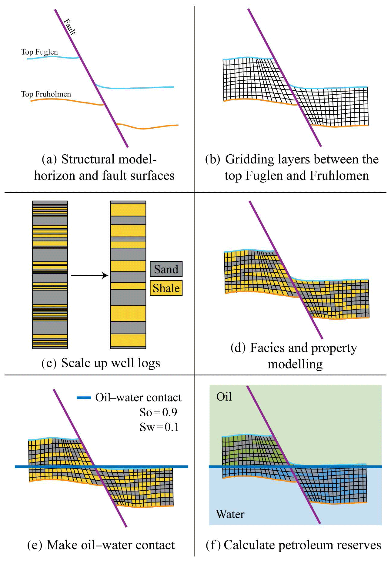
Figure 5Reservoir modelling and calculation of petroleum volume method. (a) Creation of the structural model. (b) Establishing gridded layers between the top Fuglen and top Fruholmen. (c) Upscaling of well logs from well 7120/6-1. (d) Populating facies and properties such as porosity into the individual grid cells using the upscaled well log data. (e) Drawing an oil–water contact across the study area. This OWC simulates a spill point at the lowest point of the top Fuglen. (f) Running the calculation of petroleum volumes.
For the volume calculations, there was a concern that any differences between Exps. 1 and 4 might be caused, or at least exaggerated, by the stochastic facies and porosity modelling. Different facies and porosity realizations will result in different volumes. We needed to be certain that any variations in volume were caused by the different interpretation methods and not by the stochastic property modelling. Several options were examined to negate this possibility. As the grids are identical in their i, j, and k dimensions, it was expected that Petrel™ would produce the same realization in the two grids when the same seed number was selected; this proved to be an incorrect assumption. The method selected to make sure that the same realizations were being used, and to ensure that an extreme case was not being selected, was to (1) generate 100 realizations on the Exp. 1 grid, (2) copy all 100 realizations to the Exp. 4 grid, and (3) run the volumetric analysis on all realizations for both grids. Once the volumes had been calculated for 100 realizations on each grid, they were analysed to determine the average volumes. This negated the possibility of selecting an extreme case. Using the same set of realizations in the two experiments meant that the differences in volumes could be assigned, with certainty, to the differences in interpretation methods used.
4.1 Seismic interpretation
Five seismic interpretation experiments (Fig. 3) were analysed to understand the effect that the interpretation methodology has on the resulting fault and horizon surfaces.
Firstly, it is important to consider the areal coverage and visible patterns contained in the interpretation before it is converted into surfaces (Fig. 3). When analysing the interpretation of the top Fuglen and top Fruholmen, Exps. 1–4 have an increase in interpretation density (the horizon interpretation of Exps. 4 and 5 is the same; Fig. 3a–d). All the horizon interpretations show the same general trends in topography, but as expected, the topography is more detailed and most sharply defined in the most densely interpreted data (Exps. 4 and 5; Fig. 3d, e). The top Fuglen is the most clearly imaged reflector, which resulted in complete interpretation coverage in all experiments (i.e. no gaps in the interpreted lines; Fig. 3). The clear imaging of this reflector is especially evident in the auto-tracked horizon in Exps. 4 and 5 (Fig. 3, top Fuglen). The top Fruholmen is a poorly imaged reflector, which consequently resulted in gaps in the interpreted lines (Fig. 3, top Fruholmen). The areas lacking interpretation of this reflector are evident in all experiments, but they are most clear in the auto-tracked horizon (Fig. 3d, e; top Fruholmen). The fault polygons for the two horizons do appear to have the same general trends, but this will be discussed in detail in the next section.
The horizon and fault interpretations were converted into surfaces. The horizon surfaces show the same general patterns with respect to topography in all the experiments (Fig. 6). Generally, all top Fruholmen structure maps show a topographic low on the north (hanging wall) side of each fault. The footwall blocks are uplifted relative to the hanging walls, and the points of highest elevation are located adjacent to the faults (Fig. 6, top Fruholmen). In the top Fuglen surface, the same overall topographic patterns are evident, but the amount of footwall uplift and depth of topographic lows on the hanging wall are less than on the top Fruholmen surface (Fig. 6a). The greatest differences between the experiments occur in areas where the lateral continuity of the interpretations were disrupted due to the presence of a fault, where horizon interpretations do not continue across the fault plane, and when the interpretation density was low (Exps. 1–3; Fig. 6a–c). In these cases, it is possible to identify topographic features near the faults, which are clearly artefacts (Fig. 6a–b; Exps. 1–2, white arrows).
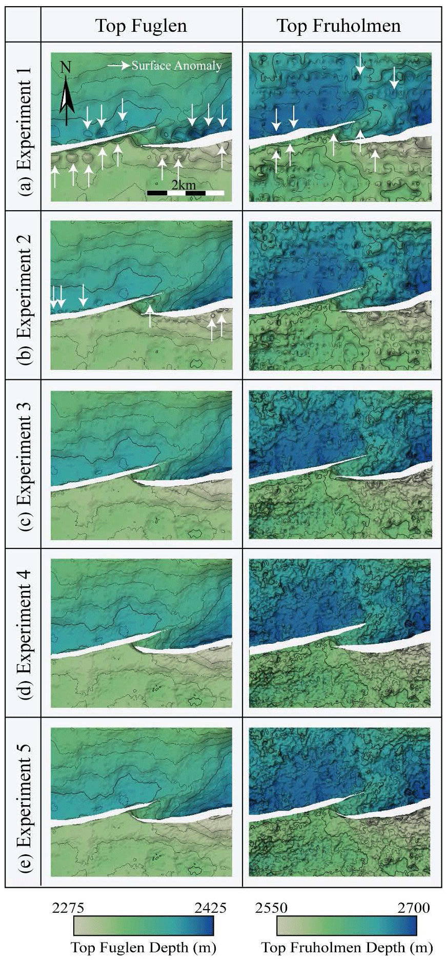
Figure 6Structure maps of the two interpreted horizons: top Fuglen and top Fruholmen (left and right columns, respectively). (a) Exp. 1 (32 IL × 32 XL interpretation, every 32nd IL fault), (b) Exp. 2 (16 × 16, every 16th IL fault), (c) Exp. 3 (8 × 8, every eighth IL fault), (d) Exp. 4 (3D auto-tracked horizons, every fourth IL fault), (e) Exp. 5 (3D auto-tracked horizons, faults every 50 m depth slice).
To better visualize the surface anomalies, thickness difference maps were generated between the surfaces of Exps. 1–3 and the most dense surfaces of Exps. 4–5. Visual inspection indicates that surfaces 1–3 all contain interpretation anomalies. The difference maps show a decrease in thickness difference with increasing interpretation density (Exps. 1–3). The maps also show that the top Fuglen surfaces are a closer match to the auto-tracked horizon than the top Fruholmen (Fig. 7).
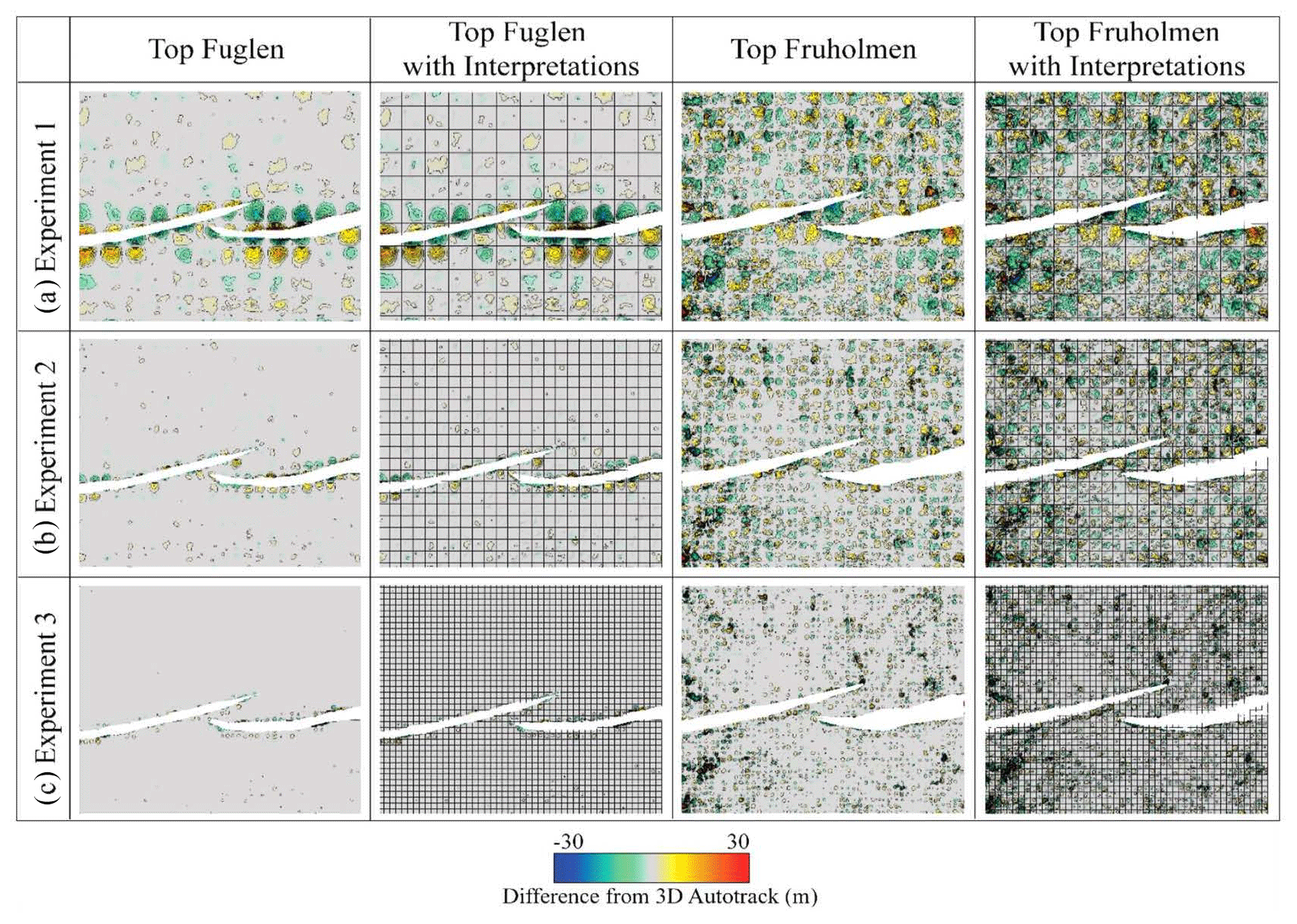
Figure 7Difference maps of the horizon surfaces for the top Fuglen and top Fruholmen in experiments 1 (a), 2 (b), and 3 (c). The auto-tracked horizon surfaces in Exps. 4 and 5 are the best-case scenario. Difference maps were computed by subtracting the experiments' interpreted horizons from the auto-tracked horizons.
Exp. 1 shows the most significant differences from the 3D auto-tracked horizons due to a sparse interpretation grid and the introduction of gridding anomalies (Fig. 7a). The thickness anomalies in both the top Fuglen and top Fruholmen can measure ± 30 m from the 3D auto-tracked surface, and the anomalous areas are up to 400 m wide and long (i.e. comparable to the interpretation spacing; Fig. 7a). The top Fuglen from Exp. 1 correlates moderately well in unfaulted areas, and all the major anomalies occur close to the faults (Fig. 7a, top Fuglen). On the hanging wall side of the faults the anomalies are predominantly depressions (i.e. a sparse interpretation grid generates a surface that is too deep), while on the footwall side the anomalies trend upward (i.e. the surface from the sparse grid is too shallow). The top Fruholmen from Exp. 1 is more anomalous across the entire surface; there is no clear correlation between the tendencies of the anomalies on the hanging wall and footwall (Fig. 7a, top Fruholmen). The areas of divergence occur in the gaps between interpreted ILs and XLs.
Exp. 2 exhibits much less significant changes in thickness with respect to the auto-tracked horizons on both the top Fuglen and top Fruholmen (Fig. 7b). For the top Fuglen, a pattern like Exp. 1 is observed; most thickness anomalies occur near the faults and correspond to gaps in the interpretation (Fig. 7b, top Fuglen). The top Fruholmen is more chaotic, but in this case the anomalies are smaller (up to 200 × 200 m) and exhibit smaller thickness differences (± 15 m) than in Exp. 1. Like in Exp. 1, the thickness differences in both the top Fuglen and Fruholmen correlate with gaps in the interpretation.
Finally, the thickness anomalies for Exp. 3 show the same trends as in Exps. 1 and 2, but again they are smaller in area (up to 100 × 100 m) and magnitude (± 5 m; Fig. 7c). The anomalies occur at points of gaps in the interpretation. The thickness anomalies in the top Fuglen are almost always observed near the faults, while those on the top Fruholmen are more widespread across the whole surface (Fig. 7c). It is important to keep in mind that the top Fuglen has complete areal coverage in the study area, while the top Fruholmen does not. In Exps. 1–3, the thickness anomalies in the top Fruholmen structure maps are in some instances linked to inconsistencies in the auto-tracked horizon.
4.2 Fault length and morphology
Fault polygons are displayed on structure maps (Fig. 6) and plotted graphically (Figs. 8, 9) to show how fault length and morphology change with the interpretation method. Generally, fault length on the interpreted horizons increases with interpretation density from Exp. 1 (shortest faults) to Exps. 4 and 5 (longest faults). These observations are clear for both the top Fuglen (Fig. 8a, b) and the top Fruholmen (Fig. 8c, d). In Exp. 5 (horizontal fault sticks), the eastern fault is longer than the fault interpreted by vertical fault sticks in Exp. 4, while the western fault is shorter than in Exp. 4 (Fig. 8).
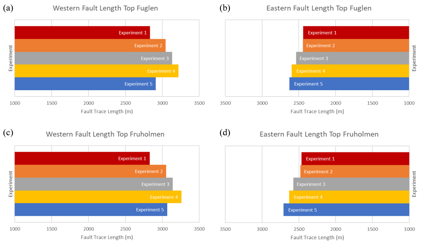
Figure 8Length of the western and eastern faults for the top Fuglen (a, b, respectively) and the top Fruholmen (c, d, respectively).
The morphology of the faults also changes with interpretation. In Exp. 1, there is a minimal amount of interaction between the two very straight faults forming the relay (Fig. 6a). In Exp. 2, the faults are also straight and do not appear to interact (Fig. 6b). In experiments 3 to 5, the northward curvature and lengthening of the eastern faults towards the western fault increase, which suggests that the relay is close to breaching or may even be breached (Fig. 6c–e). This near-breach relay is evident in the top Fuglen for Exps. 4 and 5, but it is less prominent in the top Fruholmen (Fig. 6d, e).
The effect of the interpretation method on fault length is clearly seen in the graph of fault trace distance versus fault throw (Fig. 9). The data in these graphs were sampled from the interpreted fault sticks and show that in Exp. 1 there is minimal overlap between the two faults, and the amount of overlap increases towards Exp. 4 (Fig. 9a–d). For Exp. 5, fault trace distance versus throw shows that the eastern fault is longer, while the western fault is shorter than Exp. 4 (Fig. 9e), which confirms our observations from Fig. 8.
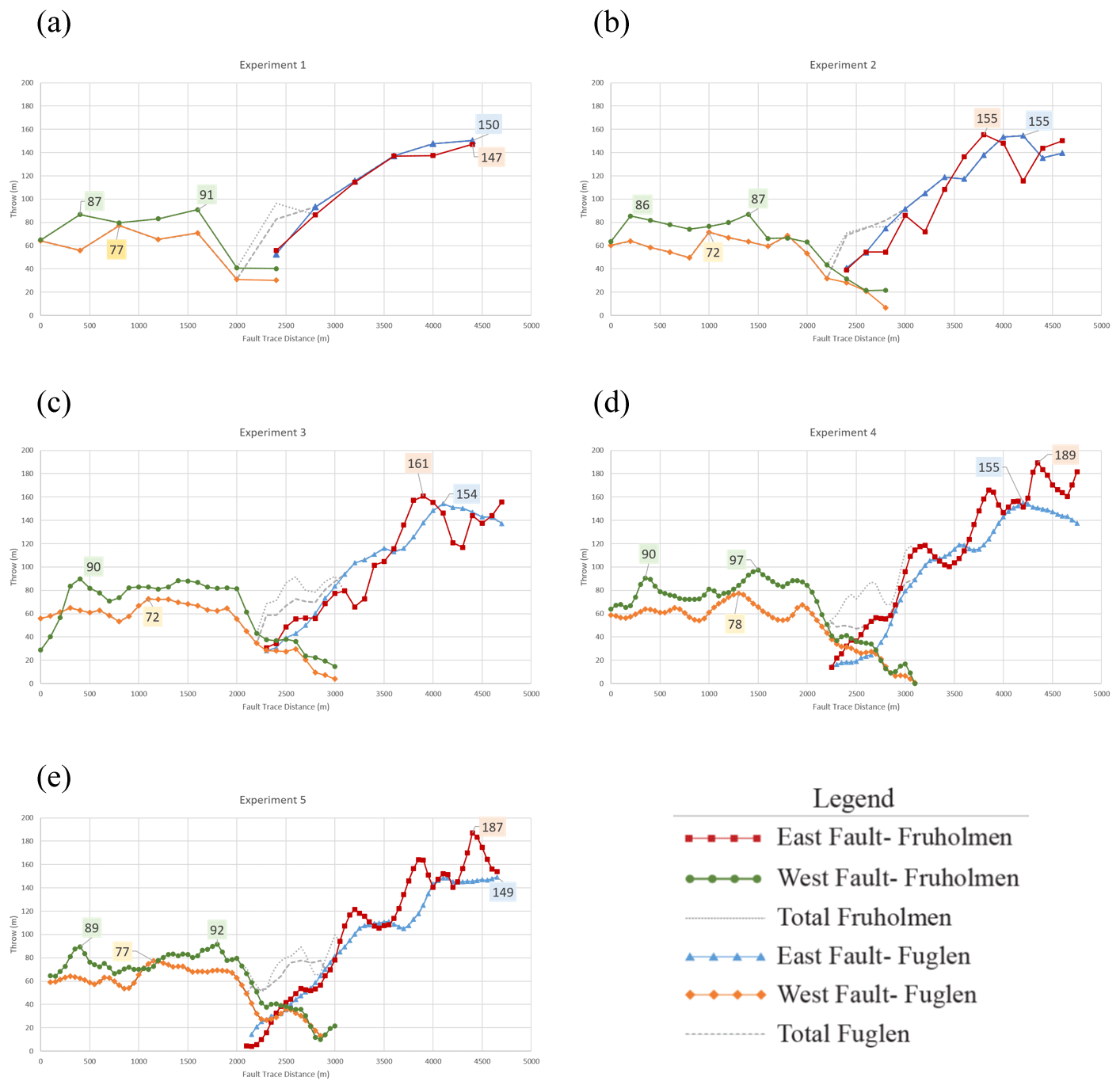
Figure 9Graphs of fault throw for Exps. 1–5 (a–e). For each experiment, fault throw was extracted to match the spacing of the interpreted fault sticks (maximum throw for each horizon is highlighted in boxes according to fault colour). In Exps. 1 (a), 2 (b), 3 (c), and 4 (d), the fault throw was extracted at 400, 200, 100, and 50 m, respectively. In Exp. 5 (e), the fault sticks are horizontal. Since it is not possible to extract the fault throw horizontally, the same sampling interval used in Exp. 4 (50 m) was used.
4.3 Fault throw
Fault throw contours from all five interpretation experiments exhibit generally consistent patterns (Fig. 4a) on the eastern and western faults but also some bullseye patterns (Fig. 10a). The western fault has similar throw magnitudes across all experiments. The lowest throws occur on the eastern margin and the highest throws (up to 100 m) on the western side. With increasing interpretation density, the throw results for this fault appear smoother and more laterally extensive. For example, in Exp. 1 the western fault shows three separate bullseye patterns, while in Exps. 2–4 it shows a progressively smoother throw distribution (Fig. 10a). For the eastern fault, the throw patterns are similar between experiments, but the throw magnitudes increase with increasing interpretation density (Fig. 10a). In Exp. 1, fault throw reaches a maximum of ∼ 150 m on the eastern side of the fault. For Exps. 2 and 3, the results have slightly higher maximum throw (∼ 175 m), but they are segmented into geologically unrealistic bullseye patterns (Fig. 10a). In Exp. 4, the maximum throw of the eastern fault is up to 200 m, and the results are more concentric, smoother, and more geologically realistic than in Exps. 1–3. Exp. 5 (fault sticks interpreted on depth slices) shows similar patterns as those observed in Exp. 4 but with more irregularities.
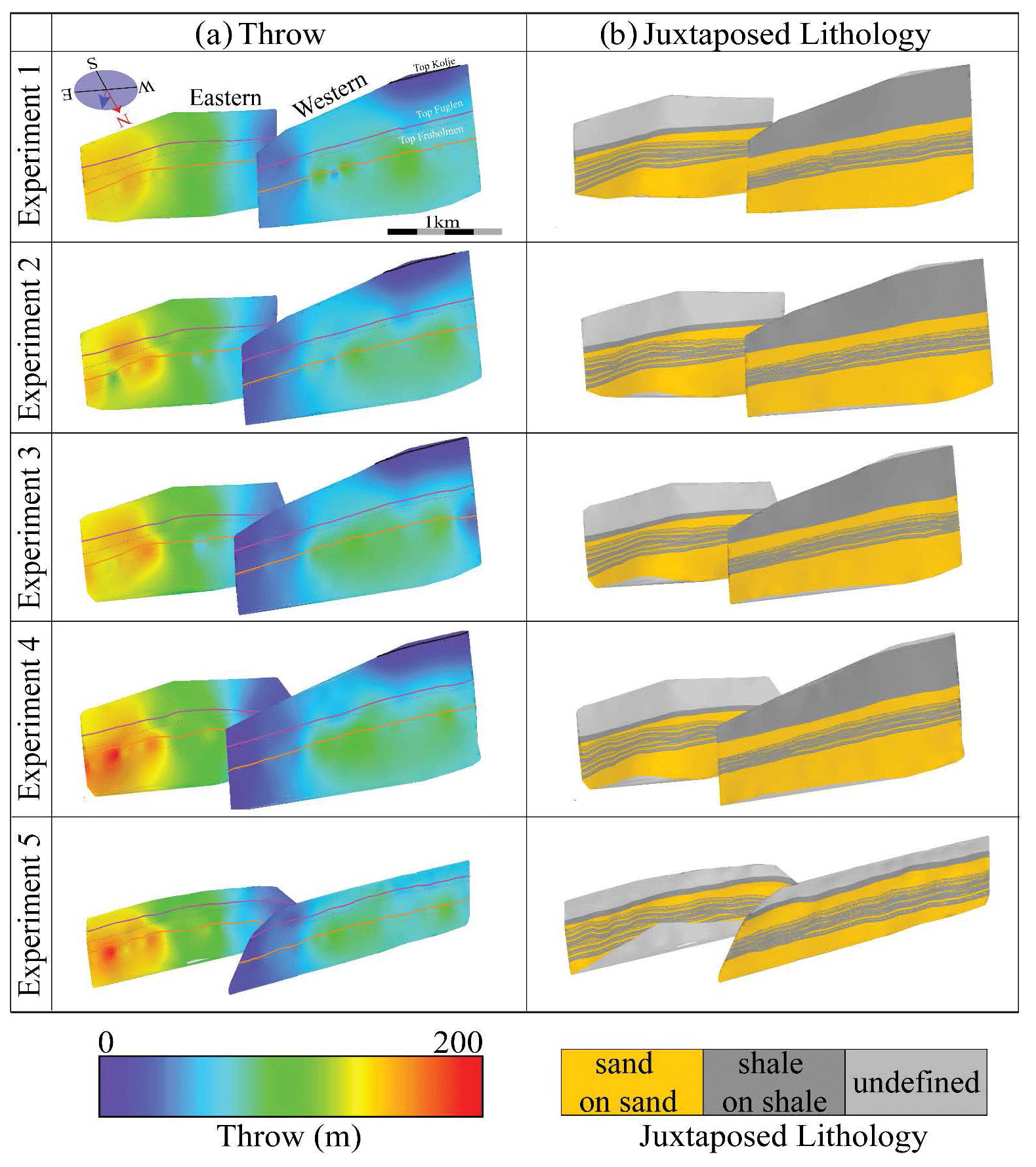
Figure 10Fault plane projections of (a) fault throw and (b) juxtaposed lithology. The projections are imaged on both the eastern and western faults for Exps. 1–5.
Fault trace distance versus throw also illustrates how fault displacement is influenced by the interpretation method (Fig. 9). As discussed before, the fault throw of all experiments is greater on the edges of the study area than near the relay (centre of the graphs in Fig. 9). For the western fault, the top Fruholmen is always displaced more than the top Fuglen. For the eastern fault, the top Fruholmen is displaced more than the top Fuglen in Exps. 4 and 5 (Fig. 9d, e), but it exhibits similar throws as the top Fuglen in Exps. 1–3 (Fig. 9a–c). In all experiments, the throw distributions for the top Fuglen are smoother than those for the top Fruholmen. This smoothness is also observable in the throw fault plane projections where the bullseye patterns occur on the top Fruholmen level. The highest throw values for the eastern fault at the top Fruholmen in Exps. 1–5 are ∼ 147, 155, 161, 189, and 187 m, respectively. These values occur near the eastern margin of the study area (Fig. 9). For the western fault, the top Fruholmen peak throw values in Exps. 1–5 are ∼ 91, 87, 90, 97, and 92 m, respectively. However, these peaks do not always fall near the western edge of the study area, as the western fault is relatively constant in throw outside the relay (Fig. 9). The top Fuglen throw on the eastern and western faults has a similar distribution as observed for the top Fruholmen (Fig. 9). At the top Fuglen level, the eastern fault has maximum throws of ∼ 150, 155, 154, 155, and 149 m, and the western fault has maximum throws of ∼ 77, 72, 72, 78, and 77 m for Exps. 1–5, respectively. Figure 9 clearly shows that the trends of throw for Exp. 1 are overly smooth, while those of Exps. 2–4 are similar. Exp. 5 shows more or less the same result as Exp. 4, with slight changes due to the extent of the faults.
4.4 Juxtaposed lithology
Lithology data projected onto the fault planes can help us to understand how interpretation methods influence the evaluation of reservoir juxtaposition and the potential for fault sealing. All experiments were populated with the same lithological data from well NO 7120/6-1 (Fig. 1b, yellow dot); the only variation is the interpretation method. On a broad scale, the juxtaposition diagrams for the five experiments look very similar on both the eastern and western faults (Fig. 10b). The uppermost section of the faults is characterized by shale–shale juxtaposition (dark grey, western fault), or it has not been characterized due to a lack of conformable top Kolje distribution on the eastern side of the study area (light grey, eastern fault). The next unit down is a homogenous sand–sand interval, followed by a shale–shale section at the fault centres, which is segmented by thin sand–sand units. Finally, the deepest lithology juxtaposition is another homogeneous sand–sand unit. On closer examination, however, comparison of the different experiments reveals that the lateral extent and definition of the intra-shale sand overlaps improve with increasing interpretation density (Fig. 10b). This is especially true when comparing the least dense seismic interpretation (Exp. 1) to the densest one (Exp. 4). Exp. 5 follows the same pattern as Exp. 4 in areas where the juxtaposed lithology ran smoothly, but there are some issues with the juxtaposition (light grey triangle at the base of the eastern fault, Fig. 10b). This anomaly is caused by a limitation in the software, whereby the horizontal interpretation of the fault on depth slices results in some sections of the fault having vertical dips. It is not possible to generate juxtaposition diagrams in these vertical fault areas.
4.5 Dip-slip gradients (longitudinal and shear strain)
Dip separation gradient (DSG) as well as longitudinal and shear strain (Freeman et al., 2010) were calculated to understand variations in interpretation confidence between the experiments. The results for the dip separation gradient are similar across all five experiments (Fig. 11a). In general, the largest DSG (> 0.2) occurs at the top Fruholmen level. The western fault has a larger distribution of high DSG values in the western top part (0.125 gradient) and a main bullseye on the eastern side (Exps. 1, 3–5; Fig. 11a). The eastern fault has the same three to four bullseyes occurring in all experiments, but Exp. 1 has the lowest DSG values.

Figure 11Fault plane projections of (a) dip separation gradient, (b) longitudinal strain, and (c) shear strain. The projections are imaged on both the eastern and western faults for Exps. 1–5.
The longitudinal strain (LS) patterns are similar to those observed in the DSG results (Fig. 11b). The colour bar for longitudinal strain is set so any values outside a geologically realistic threshold (Freeman et al., 2010) occur as red (LS >0.1) or purple (LS <−0.1). The results for LS for all experiments are similar and exhibit values that are within the defined threshold. In the western fault for Exp. 1, unrealistic LS values at the top Fruholmen level on the eastern side suggest a problem with the interpretation (Fig. 10b, top row). This problem is not present in the other experiments. High (green) LS values in the western upper half of the western fault in Exps. 1–4 are within the acceptable threshold (Fig. 10b). These high values coincide with the area between the top Kolje and top Fuglen. The eastern fault has the same LS bullseyes across its centre as observed in DSG, but they are mostly within the established threshold. In Exps. 4 and 5, there are two areas above the high LS thresholds (red) at the top Fruholmen level (Fig. 11b, black asterisks). All areas above threshold LS values (red, pink) are less than 250 m across.
For the shear strain (SS), the colour bar is also set to display geologically unrealistic values (± 0.05; red and pink, Fig. 10c) (Freeman et al., 2010). Although SS highlights more problematic areas and places more stringent constraints on the interpretation, it indicates extreme highs and lows of SS at the overlap of the western and eastern faults, respectively (Fig. 10c, black arrows). The overlapping sections of the faults are more laterally extensive from Exps. 1 through 5, which is reflected in the lateral extent of extreme SS. Localized (> 250 m) SS bullseyes highlight some slight interpretation problems discussed before in relation to LS (Fig. 11c, black asterisks). Due to the high degree of similarity between the experiments, no attempt has been made to analyse SS variations any further.
4.6 Reservoir modelling and hydrocarbon volume calculations
In order to test the implications of interpretation techniques for hydrocarbon volume calculations, the least and most densely populated experiments (Exps. 1 and 4) were input through a geological modelling workflow (Fig. 5). A 5 × 5 km geological model was generated for each experiment (Fig. 12a, b) and used to calculate the bulk rock volume, pore volume, and STOIIP (Fig. 9c, d).
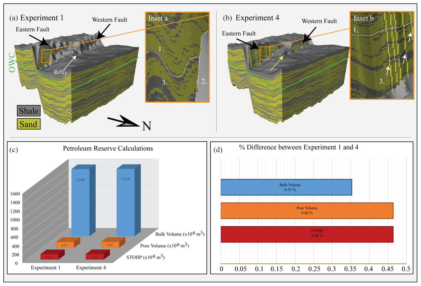
Figure 12Reservoir modelling and calculation of petroleum volumes. (a) The geological model for Exp. 1. (b) The geological model for Exp. 4. (c) Graphical representation of the petroleum volume calculations for both experiments. (d) Percent difference of the petroleum volume calculation between the experiments.
There are significant differences in fault morphology, horizon resolution, and lithology distribution between the two geological models. In Exp. 1, the surface anomalies observed in the structure maps (Sect. 4.1, Fig. 6 arrows) are also evident in the 3D grid at the top and base of the gridded interval (Fig. 12a, inset a, label 1). Since the top Fuglen and Fruholmen are used as the input to define the top and base of the gridded interval and the cells within, the surface anomalies also greatly impact the facies distribution in Exp. 1, which undulates to match these anomalies. These facies undulations can be observed on the exposed footwall of the eastern fault and on the eastern geological model boundary, as the facies pull upwards towards the footwall (Fig. 12a, inset a, label 1). In Exp. 1, there are also some problems with respect to the exposed fault planes where some shale cells have bled up and down the fault planes, creating unrealistic peaks (Fig. 12a, inset label 2). This results in poor modelling of the relay ramp structure, although the exposed footwall and hanging wall blocks appear relatively smooth (Fig. 12a, inset a, label 3).
In Exp. 4, the facies distributions do not have the same undulations that are observed in Exp. 1. This result is more or less expected since these anomalies were not evident in the top Fuglen and Fruholmen, which define the grid. Flat, more geologically representative facies distributions are clear on the uplifted footwall of the eastern and western faults, as well as on the exposed eastern boundary of the model (Fig. 12b, inset b, label 1). A “bleeding of facies” occurs on the margins of the model and slightly on the edges of the faults (Fig. 12b). The relay ramp is much more clearly defined in this experiment than in Exp. 1 (Fig. 12b, yellow arrow). The faults are better defined with respect to length and morphology, but the high density of interpreted fault sticks means that the fault planes have vertical jumps between grid cells in the 3D grid (Fig. 12b, unset b, label 3).
Bulk rock volume, pore volume, and oil (STOIIP) were calculated for both geological models using an oil–water contact of 2420 m (Fig. 12a, b; OWC). This contact was chosen to mimic a spill point at the lowest point of the top Fuglen. The volumetric analysis was run on each of the 100 realizations, and the results presented are given as their average. The stochastic facies and porosity realizations used in these calculations were identical for the two experiments, which allowed any volume differences to be assigned to the impact of the resolution of the interpretation. The volumetric calculations for Exp. 4 were always slightly larger than Exp. 1. The bulk volumes for Exps. 1 and 4 are 1548.7 and 1554.2 × 106 m3, respectively (a difference of 0.36 %). For pore volume, values of 136.8 and 137.4 × 10⁶ m3 were calculated from Exps. 1 and 4, respectively, which is a difference of 0.46 %. Finally, the calculation of oil in place (STOIIP) resulted in 123.1 × 10⁶ m3 for Exp. 1 and 123.7 × 10⁶ m3 for Exp. 4 (a difference of 0.46 %).
The volumes in Exp. 4 are slightly larger than in Exp. 1, with the increase in the bulk rock volume carried through the pore volume and STOIIP calculations. However, the percentage differences are very small: less than 0.5 % for all metrics.
5.1 Implications on horizons and faults morphologies
The seismic interpretation method had a significant impact on all aspects of the fault analysis workflow. We found that both Exps. 4 and 5 provided the most geologically accurate representation of the morphologies of horizons, faults, and their intersections. The eastern fault was longest in Exp. 5, while the western fault was longest in Exp. 4, which suggests that a combination of the methods (i.e. vertical and horizontal interpretation) would be the most rigorous approach to fault interpretation. The horizons in Exps. 4 and 5 were quick to interpret because of 3D auto-tracking, and they were also the most detailed. When interpreting the top Fuglen there was no need for a QC process since the imaging of this reflector was clear and the final surface did not contain any artefacts in the interpretation (Fig. 7, top Fuglen columns). The top Fruholmen needed some manual guidance and QC, and it did have some interpretation artefacts, but this was unavoidable due to the poor seismic quality (Fig. 7, top Fruholmen columns). The interpretation of faults was slightly more time-consuming for Exp. 5 relative to 4, but the attribute volume increased the understanding of fault morphology and length compared to Exp. 4 (see Fig. 8, fault lengths). Exp. 1 is considered to be a failure with respect to observed geological morphologies, and this methodology cannot be recommended as a method for fault interpretation, even though it was very time-efficient. The sparsity of the horizons and fault interpretations led to inaccuracies and gridding anomalies proportional to the spacing of the interpreted inlines (400 m), reduced fault length (Fig. 8, up to 400 m difference between Exps. 1 and 4, western fault), and incomplete understanding of the relay morphology. Exps. 2 and 3 were an improvement on Exp. 1, as expected. They captured some important information but not as much as Exps. 4 and 5. The differences between Exps. 2 and 3 were much less significant than those between Exps. 1 and 2. As such, if manual interpretation of faults is required, Exp. 2 should be considered the minimum acceptable interpretation density for performing a detailed fault analysis workflow.
The two aspects of the fault analysis workflow that were the most affected by the interpretation method were fault length and throw. Both the length and throw of the faults differed dramatically depending on interpretation density, which in turn had a large influence on the apparent morphologies of the faults and of the relay ramp (Figs. 8–10). The knock-on effects of these are because the fault lengths and throws impact all other aspects of the workflow. Overall, comparison of the most and least densely interpreted datasets (Exps. 4–5 and 1, respectively) shows that the length, morphology, and throws were different at both the top Fuglen and Fruholmen level (Figs. 7–10).
The impact of the interpretation method on the length, morphology, and throw profiles in the relay is critical to understand its formation. Fault displacement–throw relationships in relay ramps are dependent on the stage of relay development in question (Fig. 13). In the first stage of relay development, the faults do not overlap and therefore exhibit isolated fault throw profiles (Barnett et al., 1987; Fig. 13a–b). Stage 2 of relay development is defined by the propagation of faults to form a relay ramp (Fig. 13c). Fractures break up the ramp (that in our case are sub-seismic resolution) and accommodate some of the strain of the relay (Larsen, 1988; Peacock and Sanderson, 1994). The throw profiles of the faults interact, and the total throw of the overlapping fault segments is accommodated by the relay ramp (Peacock and Sanderson, 1994; Fig. 13d). The fault extents and throw profiles for Exp. 1 (Figs. 9a, 10a) fall somewhere between Stages 1 and 2, wherein there is a slight overlap of the faults, but a relay is only just starting to form (Fig. 6a). This is because Exp. 1 does not properly capture the full length of the fault. Stage 3 of relay development is defined as when the faults have continued to propagate and fractures have begun to spread through the relay structure, as it is near the maximum amount of strain it can accommodate (Long and Imber, 2012; Peacock and Sanderson, 1994). The propagation of the fault tips toward the relay and increased fault overlap are evident (Fig. 13e–f). Stage 4 of relay development defines the destruction (breaching) of the relay ramp and the formation of branch lines between the two relay-forming faults (Peacock and Sanderson, 1994). The original tiplines of the fault are no longer active, and the faults are now joined along branch lines formed in the weakened and sheared ramp margins (Fig. 13g–h). When analysing Exps. 4 and 5, the morphologies are comparable to those observed in Stage 3 of the relay formation. The northward propagation and curvature of the eastern fault tipline are clear, and there are likely fractures forming in the relay that are below the resolution of the seismic data. The relay in Exps. 4 and 5 has not breached on either the top Fuglen or Fruholmen level, although it is very close to breaching in Exp. 5 at the top Fuglen (Figs. 6d, e, 9d, e, 10a). The potential impact of a relay on a working hydrocarbon system and the implications of misinterpreting the relay are discussed in Sect. 5.2.
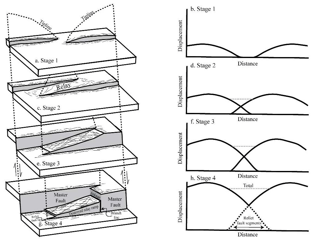
Figure 13Stages of a relay ramp and their displacement distribution. Stage 1 (a, b), Stage 2 (c, d), Stage 3 (e, f), Stage 4 (g, h). The displacement of the isolated faults in Stage 1 follows Barnett et al. (1987). Figure modified from Fachri et al. (2013a), Long and Imber (2012), Peacock and Sanderson (1994), and Rotevatn et al. (2007).
A study of longitudinal and shear strain was completed to test the accuracy of the interpretation methods (Freeman et al., 2010). According to Freeman et al. (2010), longitudinal and shear strain values in isolated faults should remain inside their defined threshold values (± 0.1 and ± 0.05, respectively) in order for the interpretation to be deemed accurate. High and low values of longitudinal and shear strain were observed across all experiments, some of which are outside these defined thresholds (Fig. 11b, c). There is a high and low shear strain accumulation in all experiments on the western and eastern faults, respectively, particularly in the parts of the faults exhibiting overlap (Fig. 11c). Freeman et al. (2010) stated that in the event of overlapping faults, higher shear strains (above their defined limit) are to be expected in the overlapping segments of the fault. The shear strain limits in this case are higher than could be expected from an isolated fault (Freeman et al., 2010). These highs and lows appear to change with interpretation density and align with the increased overlapping of the faults (Fig. 11c, double-ended black arrows). There were some bullseye patterns (longitudinal and shear strain plots) which were outside the fault overlap and outside the defined threshold strains; these are interpreted to be artefacts produced by incorrect fault stick interpretations (Fig. 11b, c black asterisks). It is possible that some of the bullseye patterns observed, which did not align with interpretation spacing, are real and linked to the coalescence of faults during their formation (e.g. Lohr et al., 2008), but this is outside the scope of this study and was not investigated further. It is important to note that interpretation accuracy with respect to longitudinal strain and shear strain was not the aim when running the initial interpretations, and therefore it is expected that some inconsistencies are present.
5.2 Implications for petroleum studies
5.2.1 Interpretation and aspects of the petroleum industry
Relay ramps and the faults that define them have a significant impact on sediment distribution pathways (deposition of reservoirs), fluid flow and migration pathways, fault seal and/or juxtaposition, and trap definition (e.g. Athmer et al., 2010; Athmer and Luthi, 2011; Botter et al., 2017; Fachri et al., 2013a; Knipe, 1997; Manzocchi et al., 2008a, 2010). By under-interpreting the relay with respect to fault length and throw (as discussed in Sect. 5.1, Exp. 1), there is a clear misunderstanding of the stage of relay development and therefore a misunderstanding of fault interactions. Exp. 1 exhibits shorter faults with less throw and therefore a less defined relay (Fig. 14, left column). This under-interpretation of the relay will also have implications for our understanding of sediment distribution pathways (Fig. 14a). Compared with the relay interpreted from Exp. 4 (Fig. 14, right column), the results of Exp. 1 (left column) also show a less laterally continuous extent of juxtaposed sand-on-sand, resulting in different fault sealing (Fig. 14b); an unsuccessful fluid flow schematic whereby petroleum does not migrate towards the producer well (Fig. 14c); and an underestimation of trap size because of the incorrect trap geometry (Fig. 14d). These results are specific for our field area and relay morphology, and of course they may differ with changing field parameters. The important thing, however, is that significant differences can be generated by applying an interpretation method that is unsuitable for the scale of the structures that are being analysed.
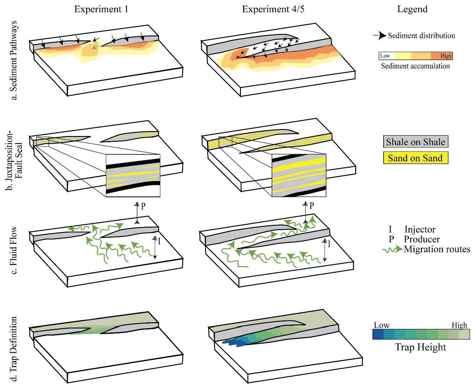
Figure 14A Comparison of sediment distribution pathways (a), lithological juxtaposition and/or fault seal (b), fluid flow (c), and trap definition (d) on an under-interpreted version of a relay (Exp. 1, column 1) and an accurate interpretation of the relay (Exp. 4, column 2). Figure based on Athmer et al. (2010), Athmer and Luthi (2011), Botter et al. (2017), Fachri et al. (2013a), Knipe (1997), Peacock and Sanderson (1994), and Rotevatn et al. (2007).
5.2.2 The effect of interpretation on geological modelling
A geological modelling workflow was run on the least and most successful interpretation methods (Exps. 1 and 4, respectively) in order to understand the impact of the interpretation method on the geological model. In Exp. 1 it is possible to identify several clear inaccuracies and problems with the model. The problems include facies undulations, which were caused by interpretation sparsity, facies bleeding on the fault planes, and the apparent under-interpretation and imaging of the relay ramp due to under-interpreted faults. The observed facies undulations can have significant implications if used in dynamic modelling such as fluid flow simulations. Since the relay is so under-interpreted in Exp. 1, the results can be expected to be false. This poor interpretation can have negative implications for the geological understanding, development, production, and drainage strategies of the field.
In this study, a major issue occurs with the apparent difference in structural morphology that is created in the model. In Exp. 1, the relay is underdeveloped due to the sparse interpretation density. Dynamic modelling of fluid flow may not exhibit correct or realistic simulations when using this experiment. Our observations support the conclusions of Jolley et al (2007), which proved the importance of properly constrained fault and horizon intersections when generating realistic geological models, and highlighted the negative impact of poor geomodelling techniques on the static model and resulting fluid flow simulations.
The bleeding of facies on the fault planes is caused by the low interpretation density and is easily avoided with a denser interpretation. Exp. 4 had more realistic horizon morphologies, more geologically realistic facies distributions, and much less facies bleed. The only problem with this interpretation was that the inline fault stick spacing resulted in linear cell anomalies and unsmooth fault planes (Fig. 12b). Therefore, we suggest that when modelling, the removal of fault sticks in the fault's centre may provide clearer results. Deleting fault sticks is likely to result in some loss of detail in the fault structural morphology such as undulations or corrugations (e.g. Needham et al., 1996; Resor and Meer, 2009; Ziesch et al., 2017). However, it is currently not possible to model these intricacies (and high density fault sticks) in a geologically realistic manner using modelling software. The optimum interpretation strategy is therefore a balance between maintaining an adequate level of geological detail and being able to produce a realistic and functioning geomodel.
Volumetric calculations using the two models revealed that the gross rock volumes were 0.35 % larger in Exp. 4 when compared to Exp. 1, and both the in-place hydrocarbon volume (STOIIP) and pore volume calculations of Exp. 4 were 0.46 % greater than Exp. 1. These differences are small (certainly much lower than the normal uncertainty values considered in the industry), which suggests that for preliminary field analysis and petroleum calculations, a detailed seismic interpretation is not all that important. However, this result has significant implications when upscaled to field dimensions – in this case the Snøhvit field. For simplicity in the calculations, we take the values from the Norwegian Petroleum Directorate for field size and the STOIIP in the entire Snøhvit area to reference an oil-only field. In reality, the field contains gas, condensate, and a small oil column (NPD, 2020). According to the Norwegian Petroleum Directorate, the Snøhvit field holds in-place volumes of ∼ 400 × 106 m3 of oil equivalent (NPD, 2020). A STOIIP difference of 0.46 % between Exps. 1 and 4 on this field size is equal to ∼ 1.84 × 10⁶ m3 of oil in place. This is equal to an underestimation of ∼ 11.6 million barrels (1 m3 oil = 6.29 b.b.l.) of in-place oil in Exp. 1 versus 4. The NPD lists the recovery factor of the Snøhvit field to be 64 % (NPD, 2020), so only 7.4 million barrels can be considered recoverable. Assuming an oil price of USD 50 per barrel, this difference in interpretation method is equivalent to ca. USD 370 million. Although this value is relatively small in the industry, it is staggering to see how inaccuracy in the calculation of petroleum reserves can be solely based on poor interpretation strategies, which are mistakes that are completely avoidable.
5.3 Recommendations for best-practice seismic interpretation
5.3.1 Horizons and horizon–fault intersections
The results showed that 3D auto-tracking (1 × 1 density) gave the best results in terms of detail in the structure of horizons and horizon–fault intersections (cutoff lines, throw, etc.), and it was the most time-efficient option assuming relatively high-quality data. In the case of high-quality data and well-defined continuous strong seismic reflectors (e.g. top Fuglen), little manual quality control of the interpretation is required. If the seismic data are of poorer quality, if the reflector in question is poorly imaged, discontinuous, or changes seismic polarity, or if there is significant structural complexity and ambiguity, then it is important to reflect on the task at hand. This is because auto-tracking algorithms may fail or generate artefacts or erroneous results that require significant manual adjustment to correct. If fault seal or juxtaposed lithologies are critical to the field analysis, then a denser manual and/or 2D auto-tracked method might be necessary and worth the significant time commitment (i.e. 8 × 8). If detailed structural analysis is not required, then a less dense (i.e. 16 × 16) grid will give sufficient results for geological interpretation. A sparse interpretation spacing (i.e. 32 × 32) can give a geologically unrealistic and inaccurate representation of the subsurface, which could lead to critical errors in prospect or field evaluations, and as such it cannot be recommended except for broad-scale regional understanding. These results assume a 12.5 m IL and XL spacing and may need to be adjusted in the event of a different spacing.
5.3.2 Faults
The results of Exps. 4 and 5 are very similar and give the most accurate picture with respect to the fault extent, throw, and morphology of the relay. When considering our experiments, it was difficult to capture the entire fault length if using less than a 4 IL interpretation spacing, but we also found interpretation from horizontal time–depth slices to be useful to accurately capture the fault length. Therefore, the recommendations are to interpret faults at a minimum of 8 or 16 IL spacing for the main body of the fault and, on approaching tiplines or complex fault intersections, to decrease the line spacing in order to capture the full length, morphologies, and relationships. We also recommend the combination of horizontal fault sticks and attributes to understand fault morphology and fault extent, as well as to keep track of fault locations in 3D when interpreting horizons. The results shown here demonstrate that less than 16 IL spacing was insufficient to capture critical details required when performing fault interpretations and as such should be avoided for critical prospect or field-scale mapping. These results also assume an IL and XL spacing of 12.5 m and may need adjustment if the data differ.
This paper has analysed the effect of the seismic interpretation method on faults, horizons, and their intersections. It also shows the implications of these interpretations for the results of a fault analysis workflow. The main findings are summarized as follows.
-
The density of fault and horizon interpretations is critical to understand fault relationships and morphologies in structure maps. 3D auto-tracked horizons, and a combination of vertical and horizontal fault sticks, give the best results for the relatively high-quality Snøhvit seismic data, with moderate to very clear continuous seismic reflectors. However, in other areas or with poorer data, a combination of auto-tracking or dense 2D interpretation grids would be required to properly capture the geological complexity.
-
Fault length is greatly impacted by the interpretation method. Special attention and denser interpretation are needed around fault tiplines.
-
The biggest effect on fault throw (and therefore much of the fault analysis workflow) was the interpretation density. If fault seal or dynamic simulation is critical, then denser vertical sticks (every 8–4 ILs) give the most accurate morphology of faults, despite needing more time and manual QC.
-
Longitudinal and shear strain are excellent for use in understanding interpretation accuracy, and their values were proven to be higher in the relay (as observed in Freeman et al., 2010). Studies of complex faulted fields and prospects should consider implementing these methods if robust fault interpretation is critical for geological understanding.
-
The effect of the interpretation method on geological modelling and the subsequent calculation of petroleum reserves showed that the importance of correct interpretation should not be underestimated. The most geologically realistic results were established when using the densest interpretation (Exp. 4). When using Exp. 1 as the model, the results were less geologically accurate (undulating facies, creeping fault cells) and led to under-interpretation of the relay, all of which has implications for dynamic modelling such as fluid flow simulations, production, and drainage strategies.
-
Calculations of petroleum reserves resulted in an underestimation of STOIIP of 0.46 % when comparing Exps. 1–4. The upscaling of this value across the Snøhvit field results in an underestimation of ∼ 11.6 million barrels or USD ∼ 370 million when comparing Exps. 1–4. Although this seems small in terms of the industry standard, this difference is only caused by inaccuracy of the seismic interpretation method. These inaccuracies in modelling and subsequent economics could be almost completely avoided by applying more robust interpretation methods.
The data and interpretations used in this work are not publicly available. The data are owned by Equinor and their partners in the Snøhvit field; special permissions were granted by them to publish this work.
JEC designed and interpreted the five experiments with contributions from NC. Both JEC and NC collaborated on the creation of the fault analysis workflow, while the application of the workflow to the five experiments was completed by JEC. CT and JEC collaborated on the design of the geomodelling workflow, its implementation, and petroleum volume calculations. RHTC aided in the implementation and upscaling of the petroleum reserve calculations, and he contributed to discussions related to the petroleum implications. JEC drafted the paper and figures with contributions and proofing from all co-authors.
The authors declare that they have no conflict of interest.
Thanks to Equinor ASA and their partners in the Snøhvit field (Petoro AS, Total E&P Norge AS, Neptune Energy AS, and Wintershall DEA AS) for providing the seismic data used in this study as well as technical guidance when analysing the data. We would also like to thank Schlumberger (Petrel™) and Badleys (T7™) for providing us with academic licenses for their software programmes and their support.
This research has been supported by the Norwegian Ministry of Education and Research.
This paper was edited by CharLotte Krawczyk and reviewed by Graham Yielding and David Tanner.
Alcalde, J., Bond, C. E., Johnson, G., Ellis, J. F., and Butler, R. W. H.: Impact of seismic image quality on fault interpretation uncertainty, GSA Today, 27, 4–10, https://doi.org/10.1130/GSATG282A.1, 2017.
Allan, U. S.: Model for hydrocarbon migration and entrapment within faulted structures, Am. Assoc. Petr. Geol. B., 73, 803–811, https://doi.org/10.1306/44b4a271-170a-11d7-8645000102c1865d, 1989.
Athmer, W. and Luthi, S. M.: The effect of relay ramps on sediment routes and deposition: A review, Sediment. Geol., 242, 1–17, https://doi.org/10.1016/j.sedgeo.2011.10.002, 2011.
Athmer, W., Groenenberg, R. M., Luthi, S. M., Donselaar, M. E., Sokoutis, D., and Willingshofer, E.: Relay ramps as pathways for turbidity currents: A study combining analogue sandbox experiments and numerical flow simulations, Sedimentology, 57, 806–823, https://doi.org/10.1111/j.1365-3091.2009.01120.x, 2010.
Badley, M. E. E., Freeman, B., Roberts, A. M., Thatcher, J. S., Walsh, J. J., Watterson, J., and Yielding, G.: Fault interpretation during seismic interpretation and reservoir evaluation, in: The Integration of Geology, Geophysics, Petrophysics and Petroleum Engineering in Reservoir Delineation, Description and Management, 224–241, available at: http://archives.datapages.com/data/specpubs/resmi1/data/a164/a164/0001/0200/0224.htm, 1991.
Bakker, P.: Image structure analysis for seismic interpretation, Technische Universiteit Delft, available at: http://citeseerx.ist.psu.edu/viewdoc/download?doi=10.1.1.105.4677&rep=rep1&type=pdf (last access: September 2020), 2002.
Barnett, J. A. M., Mortimer, J., Rippon, J. H., Walsh, J. J., and Watterson, J.: Displacement geometry in the volume containing a single normal fault, Am. Assoc. Petr. Geol. B., 71, 925–937, 1987.
Bond, C. E.: Uncertainty in structural interpretation: Lessons to be learnt, J. Struct. Geol., 74, 185–200, https://doi.org/10.1016/j.jsg.2015.03.003, 2015.
Bond, C. E., Philo, C., and Shipton, Z. K.: When there isn't a right answer: Interpretation and reasoning, key skills for twenty-first century geoscience, Int. J. Sci. Educ., 33, 629–652, https://doi.org/10.1080/09500691003660364, 2011.
Bond, E. C., Shipton, Z. K., and Jones, S.: What do you think this is? Conceptual Uncertainty in Geoscience Interpretation, GSA Today, 17, https://doi.org/10.1130/GSAT01711A.1, 2007., 2007.
Botter, C., Cardozo, N., Hardy, S., Lecomte, I., and Escalona, A.: From mechanical modeling to seismic imaging of faults: A synthetic workflow to study the impact of faults on seismic, Mar. Pet. Geol., 57, 187–207, https://doi.org/10.1016/j.marpetgeo.2014.05.013, 2014.
Botter, C., Cardozo, N., Hardy, S., Lecomte, I., Paton, G., and Escalona, A.: Seismic characterisation of fault damage in 3D using mechanical and seismic modelling, Mar. Pet. Geol., 77, 973–990, https://doi.org/10.1016/j.marpetgeo.2016.08.002, 2016a.
Botter, C., Cardozo, N., Hardy, S., Lecomte, I., Paton, G., and Escalona, A.: Seismic characterization of fault damage in 3D using mechanical and seismic modelling, Mar. Pet. Geol., 77, 973–990, 2016b.
Botter, C., Cardozo, N., Lecomte, I., Rotevatn, A., and Paton, G.: The impact of faults and fluid flow on seismic images of a relay ramp over production time, Pet. Geosci., 23, 17–28, 2017.
Bretan, P., Yielding, G., Mathiassen, O. M., and Thorsnes, T.: Fault-seal analysis for CO2 storage: An example from the troll area, norwegian continental shelf, Pet. Geosci., 17, 181–192, https://doi.org/10.1144/1354-079310-025, 2011.
Cader, A.: Rapid Generation of Fault Sticks from an Existing Adaptive Fault Interpretation, Geoteric Blog, available at: https://blog.geoteric.com/ (last access: 25 April 2020), 2018.
Caine, J. S., Evans, J. P., and Forster, C. B.: Fault zone architecture and permeability structure, Geology, 24, 1025–1028, 1996.
Cerveny, K., Davies, R., Dudley, G., Fox, R., Kaufman, P., Knipe, R. J. J. and Krantz, B.: Reducing uncertainty with fault-seal analysis, Oilf. Rev., 38–51, available at: http://www.slb.com/~/media/Files/resources/oilfield_review/ors04/win04/04_fault_seal_analysis.pdf (September 2020), 2004.
Cunningham, J., Cardozo, N., Townsend, C., Iacopini, D., and Wærum, G. O.: Fault deformation, seismic amplitude and unsupervised fault facies analysis: Snøhvit Field, Barents Sea, J. Struct. Geol., 118, 165–180, https://doi.org/10.1016/j.jsg.2018.10.010, 2019.
Cunningham, J., Cardozo, N., Weibull, W. W., and Iacopini, D.: Investigating the seismic imaging of faults using PS data from the Snøhvit field, Barents Sea and forward seismic modelling, Petroleum Geoscience, submitted, 2021.
Davatzes, N. C. and Aydin, A.: Distribution and nature of fault architecture in a layered sandstone and shale sequence: An example from the Moab fault, Utah, AAPG Mem., , 153–180, 2005.
Dee, S., Freeman, B., Yielding, G., Roberts, A., and Bretan, P.: Best practice in structural geological analysis, First Break, 23, 49–54, https://doi.org/10.3997/1365-2397.23.4.26500, 2005.
Doré, A. G.: Barents Sea Geology, Petroleum Resources and Commercial Potential, Arctic, 48, 207–221, 1995.
Dutzer, J.-F., Basford, H., and Purves, S.: Investigating fault-sealing potential through fault relative seismic volume analysis, Pet. Geol. Conf. Ser., 7, 509–515, 2010.
Edmundson, I., Rotevatn, A., Davies, R., Yielding, G., and Broberg, K.: Key controls on hydrocarbon retention and leakage from structural traps in the Hammerfest Basin, SW Barents Sea: implications for prospect analysis and risk assessment, Pet. Geosci., 26, 589–606, https://doi.org/10.1144/petgeo2019-094, 2019.
Elliott, G. M., Wilson, P., Jackson, C. A. L., Gawthorpe, R. L., Michelsen, L., and Sharp, I. R.: The linkage between fault throw and footwall scarp erosion patterns: An example from the Bremstein Fault Complex, offshore Mid-Norway, Basin Res., 24, 180–197, 2012.
Fachri, M., Rotevatn, A., and Tveranger, J.: Fluid flow in relay zones revisited: Towards an improved representation of small-scale structural heterogeneities in flow models, Mar. Pet. Geol., 46, 144–164, https://doi.org/10.1016/j.marpetgeo.2013.05.016, 2013a.
Fachri, M., Tveranger, J., Braathen, A., and Schueller, S.: Sensitivity of fluid flow to deformation-band damage zone heterogeneities: A study using fault facies and truncated gaussian simulation, J. Struct. Geol., 52, 60–79, https://doi.org/10.1016/j.jsg.2013.04.005, 2013b.
Fachri, M., Tveranger, J., Braathen, A., and Røe, P.: Volumetric faults in field-sized reservoir simulation models: A first case study, Am. Assoc. Petr. Geol. B., 100, 795–817, https://doi.org/10.1306/02011614118, 2016.
Fisher, Q. J. and Knipe, R. J.: Fault sealing processes in siliciclastic sediments, Geol. Soc. Spec. Publ., 147, 117–134, https://doi.org/10.1144/GSL.SP.1998.147.01.08, 1998.
Fossen, H. and Rotevatn, A.: Fault linkage and relay structures in extensional settings-A review, Earth-Sci. Rev., 154, 14–28, https://doi.org/10.1016/j.earscirev.2015.11.014, 2016.
Freeman, B., Yielding, G., and Badley, M.: Fault correlation during seismic interpretation, First Break, 8, 87–95, https://doi.org/10.3997/1365-2397.1990006, 1990.
Freeman, B., Boult, P. J., Yielding, G., and Menpes, S.: Using empirical geological rules to reduce structural uncertainty in seismic interpretation of faults, J. Struct. Geol., 32, 1668–1676, https://doi.org/10.1016/j.jsg.2009.11.001, 2010.
Gudlaugsson, S. T., Faleide, J. I., Johansen, S. E., and Breivik, A. J.: Late Palaeozoic structural developments of the south-western Barents Sea, Mar. Pet. Geol., 15, 73–102, https://doi.org/10.1016/S0264-8172(97)00048-2, 1998.
Gupta, S., Underhill, J. R., Sharp, I. R., and Gawthorpe, R. L.: Role of fault interactions in controlling synrift sediment dispersal patterns: Miocene, Abu Alaqa Group, Suez Rift, Sinai, Egypt, Basin Res., 11, 167–189, https://doi.org/10.1046/j.1365-2117.1999.00300.x, 1999.
Iacopini, D. and Butler, R. W. H.: Imaging deformation in submarine thrust belts using seismic attributes, Earth Planet. Sci. Lett., 302, 414–422, https://doi.org/10.1016/j.epsl.2010.12.041, 2011.
Iacopini, D., Butler, R. W. H., and Purves, S.: Seismic imaging of thrust faults and structural damage: A visualization workflow for deepwater thrust belts, First Break, 30, 77–84, doi:0.3997/1365-2397.30.5.58681, 2012.
Jolley, S. J., Dijk, H., Lamens, J. H., Fisher, Q. J., Manzocchi, T., Eikmans, H., and Huang, Y.: Faulting and fault sealing in production simulation models: Brent Province, northern North Sea, Pet. Geosci., 13, 321–340, https://doi.org/10.1144/1354-079306-733, 2007.
Knipe, R. J.: Faulting processes and fault seal, Nor. Pet. Soc. Spec. Publ., 1, 325–342, https://doi.org/10.1016/B978-0-444-88607-1.50027-9, 1992.
Knipe, R. J. J.: Juxtaposition and seal diagrams to help analyze fault seals in hydrocarbon reservoirs, Am. Assoc. Petr. Geol. B., 81, 187–195, https://doi.org/10.1306/522B42DF-1727-11D7-8645000102C1865D, 1997.
Larsen, P.-H.: Relay structures in a Lower Permian basement-involved extension system, East Greenland, J. Struct. Geol., 10, 3–8, https://doi.org/10.1016/0191-8141(88)90122-8, 1988.
Linjordet, A. and Olsen, R. G.: The Jurassic Snøhvit gas field, Hammerfest basin, offshore northern Norway, in Giant oil and gas fields of the decade 1978–1988, Am. Assoc. Petr. Geol., 3, 349–370, https://doi.org/10.1306/M54555C21, 1992.
Lohr, T., Krawczyk, C. M., Oncken, O., and Tanner, D. C.: Evolution of a fault surface from 3D attribute analysis and displacement measurements, J. Struct. Geol., 30, 690–700, https://doi.org/10.1016/j.jsg.2008.02.009, 2008.
Long, J. J. and Imber, J.: Geometrically coherent continuous deformation in the volume surrounding a seismically imaged normal fault-array, J. Struct. Geol., 32, 222–234, https://doi.org/10.1016/j.jsg.2009.11.009, 2010.
Long, J. J. and Imber, J.: Strain compatibility and fault linkage in relay zones on normal faults, J. Sediment. Petrol., 36, 16–26, https://doi.org/10.1016/j.jsg.2011.12.013, 2012.
Manzocchi, T., Heath, A. E., Palananthakumar, B., Childs, C., and Walsh, J. J.: Faults in conventional flow simulation models: a consideration of representational assumptions and geological uncertainties, Pet. Geosci., 14, 91–110, https://doi.org/10.1144/1354-079306-775, 2008a.
Manzocchi, T., Carter, J. N., Skorstad, A., Fjellvoll, B., Stephen, K. D., Howell, J. A., Matthews, J. D., Walsh, J. J., Nepveu, M., Bos, C., Cole, J., Egberts, P., Flint, S., Hern, C., Holden, L., Hovland, H., Jackson, H., Kolbjörnsen, O., MacDonald, A., Nell, P. A. R., Onyeagoro, K., Strand, J., Syversveen, A. R., Tchistiakov, A., Yang, C., Yielding, G., and Zimmerman, R. W.: Sensitivity of the impact of geological uncertainty on production from faulted and unfaulted shallow-marine oil reservoirs: Objectives and methods, Pet. Geosci., 14, 3–15, https://doi.org/10.1144/1354-079307-790, 2008b.
Manzocchi, T., Childs, C., and Walsh, J. J.: Faults and fault properties in hydrocarbon flow models, Geofluids, 10, 94–113, https://doi.org/10.1111/j.1468-8123.2010.00283.x, 2010.
Miocic, J. M., Johnson, G., and Bond, C. E.: Uncertainty in fault seal parameters: implications for CO2 column height retention and storage capacity in geological CO2 storage projects, Solid Earth, 10, 951–967, https://doi.org/10.5194/se-10-951-2019, 2019.
Needham, D. T., Yielding, G., and Freeman, B.: Analysis of fault geometry and displacement patterns, Geol. Soc. Spec. Publ., 99, 189–199, https://doi.org/10.1144/GSL.SP.1996.099.01.15, 1996.
NPD: Snøhvit Field Overview, Norwegian Petroleum Directorate, available at: https://factpages.npd.no/en/field/pageview/all/2053062, last access: 30 April 2020.
Ostanin, I., Anka, Z., di Primio, R., and Bernal, A.: Identification of a large Upper Cretaceous polygonal fault network in the Hammerfest basin: Implications on the reactivation of regional faulting and gas leakage dynamics, SW Barents Sea, Mar. Geol., 332–334, 109–125, https://doi.org/10.1016/j.margeo.2012.03.005, 2012.
Peacock, D. C. P. and Sanderson, D. J.: Geometry and development of relay ramps in normal fault systems, Am. Assoc. Petr. Geol. B, 78, 147–165, https://doi.org/10.1306/BDFF9046-1718-11D7-8645000102C1865D, 1994.
Peacock, D. C. P., Nixon, C. W., Rotevatn, A., Sanderson, D. J., and Zuluaga, L. F.: Glossary of fault and other fracture networks, J. Struct. Geol., 92, 12–29, https://doi.org/10.1016/j.jsg.2016.09.008, 2016.
Resor, P. G. and Meer, V. E.: Slip heterogeneity on a corrugated fault, Earth Planet. Sci. Lett., 288, 483–491, https://doi.org/10.1016/j.epsl.2009.10.010, 2009.
Richards, F. L., Richardson, N. J., Bond, C. E., and Cowgill, M.: Interpretational variability of structural traps: implications for exploration risk and volume uncertainty, Geol. Soc. Spec. Publ., 421, 7–27, https://doi.org/10.1144/SP421.13, 2015.
Rippon, J. H.: Contoured patterns of the throw and hade of normal faults in the Coal Measures (Westphalian) of north-east Derbyshire, Proc. Yorksh. Geol. Soc., 45, 147–161, https://doi.org/10.1144/pygs.45.3.147, 1985.
Rotevatn, A., Fossen, H., Hesthammer, J., Aas, T. E., and Howell, J. A.: Are relay ramps conduits for fluid flow? Structural analysis of a relay ramp in Arches National Park, Utah, Geol. Soc. Spec. Publ., 270, 55–71, https://doi.org/10.1144/GSL.SP.2007.270.01.04, 2007.
Schaaf, A. and Bond, C. E.: Quantification of uncertainty in 3-D seismic interpretation: implications for deterministic and stochastic geomodeling and machine learning, Solid Earth, 10, 1049–1061, https://doi.org/10.5194/se-10-1049-2019, 2019.
Shuey, R. T.: A simplification of the Zoeppritz equations, Geophysics, 50, 609–614, https://doi.org/10.1190/1.1441936, 1985.
Solum, J. G., Jolley, S. J., and Meyer, B. D.: Increasing Interpreter Capability in Structurally Complex Settings through Combined Field Work, Interpretation, and Geocellular Modeling, in 3-D structural interpretation: Earth, mind, and machine: AAPG Memoir, 111, 191–218, 2016.
Sund, T., Skarpnes, O., Nørgård Jensen, L., and Larsen, R. M.: Tectonic development and hydrocarbon potential offshore Troms, Northern Norway, in: AAPG Spec. Pub. Memoir: Future Petroleum Provinces of the World, 40, 615–627, 1984.
Townsend, C., Firth, I. R., Westerman, R., Kirkevollen, L., Harde, M., and Andersen, T.: Small seismic-scale fault identification and mapping, in Faulting, Fault Sealing and Fluid Flow in Hydrocarbon Reservoirs, Geol. Soc. Spec. Pub., 147, 1–25, 1998.
Turner, A. K.: Challenges and trends for geological modelling and visualisation, B. Eng. Geol. Environ., 65, 109–127, https://doi.org/10.1007/s10064-005-0015-0, 2006.
Walsh, J. J. and Watterson, J.: Distributions of cumulative displacement and seismic slip on a single normal fault surface, J. Struct. Geol., 9, 1039–1046, https://doi.org/10.1016/0191-8141(87)90012-5, 1987.
Walsh, J. J. and Watterson, J.: Analysis of the relationship between displacements and dimensions of faults, J. Struct. Geol., 10, 239–247, https://doi.org/10.1016/0191-8141(88)90057-0, 1988.
Walsh, J. J. and Watterson, J.: Displacement gradients on fault surfaces, J. Struct. Geol., 11, 307–316, https://doi.org/10.1016/0191-8141(89)90070-9, 1989.
Walsh, J. J. and Watterson, J.: New methods of fault projection for coalmine planning, Proc. Yorksh. Geol. Soc., 42, 209–219, https://doi.org/10.1144/pygs.48.2.209, 1990.
Watterson, J.: Fault dimensions, displacements and growth, Pure Appl. Geophys. Pageoph., 124, 365–373, https://doi.org/10.1007/BF00875732, 1986.
Wilson, P., Hodgetts, D., Rarity, F., Gawthorpe, R. L., and Sharp, I. R.: Structural geology and 4D evolution of a half-graben: New digital outcrop modelling techniques applied to the Nukhul half-graben, Suez rift, Egypt, J. Struct. Geol., 31, 328–345, https://doi.org/10.1016/j.jsg.2008.11.013, 2009.
Wilson, P., Elliott, G. M., Gawthorpe, R. L., Jackson, C. a. L., Michelsen, L., and Sharp, I. R.: Geometry and segmentation of an evaporite-detached normal fault array: 3D seismic analysis of the southern Bremstein Fault Complex, offshore mid-Norway, J. Struct. Geol., 51, 74–91, https://doi.org/10.1016/j.jsg.2013.03.005, 2013.
Wood, A. M., Paton, D. A., and Collier, R. E. L. L. L.: The missing complexity in seismically imaged normal faults: what are the implications for geometry and production response?, Geol. Soc. Spec. Publ., 421, 1–18, https://doi.org/10.1144/SP421.12, 2015.
Yielding, G. and Freeman, B.: 3-D Seismic-Structural Workflows – Examples Using the Hat Creek Fault System, in: 3-D Structural Interpretation, edited by: Krantz, B. Ormand, C., and Freeman, B., Am. Assoc. Petr. Geol., USA, 155–171, 2016.
Yielding, G., Freeman, B., and Needham, D. T.: Quantitative fault seal prediction, Am. Assoc. Petr. Geol. B., 81, 897–917, https://doi.org/10.1306/522B498D-1727-11D7-8645000102C1865D, 1997.
Ziesch, J., Aruffo, C. M., Tanner, D. C., Beilecke, T., Dance, T., Henk, A., Weber, B., Tenthorey, E., Lippmann, A., and Krawczyk, C. M.: Geological structure and kinematics of normal faults in the Otway Basin, Australia, based on quantitative analysis of 3-D seismic reflection data, Basin Res., 29, 129–148, https://doi.org/10.1111/bre.12146, 2017.