the Creative Commons Attribution 4.0 License.
the Creative Commons Attribution 4.0 License.
 | 02 Nov 2022
Geophysical analysis of an area affected by subsurface dissolution – case study of an inland salt marsh in northern Thuringia, Germany
Sonja H. Wadas
Hermann Buness
Raphael Rochlitz
Peter Skiba
Thomas Günther
Michael Grinat
David C. Tanner
Ulrich Polom
Gerald Gabriel
Charlotte M. Krawczyk
The subsurface dissolution of soluble rocks can affect areas over a long period of time and pose a severe hazard. We show the benefits of a combined approach using P-wave and SH-wave reflection seismics, electrical resistivity tomography, transient electromagnetics, and gravimetry for a better understanding of the dissolution process. The study area, “Esperstedter Ried” in northern Thuringia, Germany, located south of the Kyffhäuser hills, is a large inland salt marsh that developed due to dissolution of soluble rocks at approximately 300 m depth. We were able to locate buried dissolution structures and zones, faults and fractures, and potential fluid pathways, aquifers, and aquitards based on seismic and electromagnetic surveys. Further improvement of the model was accomplished by analyzing gravimetry data that indicates dissolution-induced mass movement, as shown by local minima of the Bouguer anomaly for the Esperstedter Ried. Forward modeling of the gravimetry data, in combination with the seismic results, delivered a cross section through the inland salt marsh from north to south. We conclude that tectonic movements during the Tertiary, which led to the uplift of the Kyffhäuser hills and the formation of faults parallel and perpendicular to the low mountain range, were the initial trigger for subsurface dissolution. The faults and the fractured Triassic and lower Tertiary deposits serve as fluid pathways for groundwater to leach the deep Permian Zechstein deposits, since dissolution and erosional processes are more intense near faults. The artesian-confined saltwater rises towards the surface along the faults and fracture networks, and it formed the inland salt marsh over time. In the past, dissolution of the Zechstein formations formed several, now buried, sagging and collapse structures, and, since the entire region is affected by recent sinkhole development, dissolution is still ongoing. From the results of this study, we suggest that the combined geophysical investigation of areas prone to subsurface dissolution can improve the knowledge of control factors, hazardous areas, and thus local dissolution processes.
- Article
(15452 KB) - Full-text XML
- BibTeX
- EndNote


The subsurface dissolution or leaching of soluble rocks poses a major geohazard, especially if it occurs in urbanized areas (Gutiérrez et al., 2014; Parise, 2015a). In particular, the formation of sinkholes, also called dolines, can cause building and infrastructure damage as well as life-threatening situations (Beck, 1988; Waltham et al., 2005; Parise et al., 2015b). Therefore, gaining a better understanding of the dissolution process, its controlling factors, and the resulting structures is of high importance.
The subsurface dissolution process requires the presence of soluble rocks (e.g., evaporites), unsaturated groundwater, or meteoric water, as well as fractures, joints, or faults which may serve as fluid pathways (Davies, 1951; White and White, 1969; Waltham et al., 2005; De Waele et al., 2017). In general, this process can form different kinds of sinkhole types. The most recent sinkhole classification proposed by Gutiérrez et al. (2014), which integrates the classification schemes by, e.g., Beck (2005), Waltham et al. (2005), and Gutiérrez et al. (2008) and was updated by, e.g., Parise (2019) and Parise (2022), groups them into two categories: solution sinkholes and subsidence sinkholes. Solution sinkholes are formed due to lowering of the ground surface caused by corrosion of exposed soluble rocks, and subsidence sinkholes are generated by both subsurface dissolution and downward gravitational mass movement. Subsidence sinkholes can be further subdivided based on affected materials (cover, bedrock, and caprock) and the subsidence mechanisms (collapse, sagging, and suffosion). Collapse sinkholes are characterized by brittle deformation and upward-migrating cavities and rock failure, finally resulting in sudden collapse of the ground surface with steep edges. Sagging sinkholes are caused by passive bending of sediments due to differential dissolution and the lack of basal support. A large difference compared to the other types of subsidence sinkholes is that no cavities are required to generate a sagging sinkhole. And suffosion sinkholes develop due to the downward migration of unconsolidated sediments through voids. In nature, however, sinkholes are often not so easy to classify, as they often have a polygenetic origin.
Several studies have dealt with the understanding of the processes and the imaging of subsurface dissolution structures, such as cavities, sinkholes, and depressions, using different types of methods. The most suitable methods for the monitoring of sinkhole development are aerial photos, differential GPS, and radar interferometry (Yechieli et al., 2002; Abelson et al., 2003; Iovine et al., 2010; Abou Karaki et al., 2019; Watson et al., 2019; Zumpano et al., 2019; Vey et al., 2021). For the detection of cavities and mass movement, gravimetric methods have been shown to be useful (Neumann, 1977; Butler, 1984), as they also deliver information about possible cavity fills, as does electrical resistivity tomography (ERT) in addition to various electromagnetic methods (Militzer et al., 1979; Bosch and Müller, 2001; Miensopust et al., 2015; Kaufmann et al., 2018). To obtain an image of the subsurface the most common techniques are ground-penetrating radar (Kaspar and Pecen, 1975; Batayneh et al., 2002) and reflection seismics (Steeples et al., 1986; Miller and Steeples, 2008; Krawczyket al., 2012; Margiotta et al., 2016; Wadas et al., 2016). Several studies in karst regions using P-wave reflection seismics have been carried out (Evans et al., 1994; Keydar et al., 2012), but investigations using SH-wave reflection seismics that enable high-resolution imaging of the near surface (Krawczyket al., 2012; Wadas et al., 2016, 2017; Polom et al., 2018), or even in combination with P waves, are sparse or missing. Since subsurface dissolution and the development of its corresponding structures are complex phenomena, a combination of various methods (e.g., Malehmir et al., 2016; Al-Halbouni et al., 2021; Ezersky et al., 2021) is needed to better understand the components and associated controlling factors. The more boundary conditions that constrain the processes and structures that can be determined, the better, e.g., dynamic models (Augarde et al., 2003, 2019) can be adapted in order to make better predictions of hazardous areas.
In this study, we show the benefits of a combined approach using P- and SH-wave reflection seismics including ERT (Doetsch et al., 2012; Wiederhold et al., 2013; Ronczka et al., 2017; Nickschick et al., 2019; Tanner et al., 2020), transient electromagnetics (TEMs; Rochlitz et al., 2018; Steuer et al., 2011), and gravimetry (Eppelbaum et al., 2008; Ezersky et al., 2013b; Flechsig et al., 2015) to better understand the local subsurface dissolution of an inland salt marsh in Thuringia, Germany. We analyze different types of subsidence sinkholes, like collapse sinkholes and depressions or sagging sinkholes, and determine the vertical and lateral fluid pathways and areas of subsurface mass movement. Furthermore, we recommend a workflow for geophysical investigation of areas prone to subsurface dissolution and sinkhole development, as well as to determine control factors and hazardous areas.
Germany suffers from a widespread sinkhole problem because soluble deposits are close to the surface in many areas (Goldscheider and Bechtel, 2009; Krawczyket al., 2012; Kaufmann, 2014; Wadas et al., 2016; Kaufmann et al., 2018). One of the main areas affected by subsurface dissolution is located along the Kyffhäuser Southern Margin Fault (KSMF) in Thuringia. The Esperstedter Ried to the south of the Kyffhäuser hills is part of this area. It is a 5 km2 wide sag, and it is the largest inland salt marsh of Thuringia (Fig. 1). It developed due to leaching of salt-bearing rocks at approximately 300 m depth (Schriel and Bülow, 1926a, b).
2.1 Geological evolution
The Kyffhäuser hills have a N–S extension of 6 km and a W–E extension of 13 km, and they are one of the smallest low mountain ranges in Germany. To the south, the hills are bounded by the northward-dipping, W–E-striking KSMF, a major thrust fault (Schriel and Bülow, 1926a, b).
An epicontinental ocean, the Zechstein Sea, covered the area during the Permian, and due to sea level changes, conglomerates, carbonates, sulfates, and salt were cyclically deposited (Richter-Bernburg, 1953). They were formed by chemical precipitation, and according to solubility, carbonates (calcite, dolomite) were precipitated first, then sulfates (gypsum), and finally chlorides (rock salt, potassium salt, and magnesium salt). The latter is extremely soluble and therefore absent in some parts of the study area nowadays. Regarding the sulfates, dehydration, e.g., during burial, can transform gypsum into anhydrite, but in the case of hydration, e.g., during exhumation, the reverse transformation is also possible (Waltham et al., 2005). As a result, the central part of the Kyffhäuser hills consists of sandstones and conglomerates, and the southern part consists of gypsum and anhydrite. The main Zechstein formations south of the hills are the Werra, Staßfurt, and Leine formations (z1–z3). Anhydrite and gypsum of z1 to z2 formations represent the main horizon affected by dissolution in the research area (Schriel and Bülow, 1926a, b). The erosion of the Variscan Orogen at the Permian–Carboniferous transition led to deposition of eroded material in the Molasse Basin, and today these clastic sediments form the central part of the Kyffhäuser hills (Schriel, 1922; Knoth and Schwab, 1972). Triassic deposits are only found at isolated locations, and Cretaceous and Jurassic rocks have been completely eroded (Schriel and Bülow, 1926a, b; Reuter, 1962). During the Upper Cretaceous and the Tertiary, the low mountain range was uplifted and tilted, which resulted in the formation of a fault scarp to the north and a southward-dipping terrain (Freyberg, 1923). Tertiary deposits are found near Bad Frankenhausen and Esperstedt, and Quaternary sediments, such as silt and loess, cover a large area (Schriel and Bülow, 1926a, b).
The presence of salt springs and the occurrence of sinkholes and depressions in the near surface indicate soluble rocks in the underground such as the Zechstein formations, and they show that Bad Frankenhausen and Esperstedt are affected by subsurface dissolution (Reuter, 1962).

Figure 1Geological map showing the Esperstedter Ried (modified after Schriel and Bülow, 1926a, b). The black box marks the investigation area.
2.2 Stratigraphy
Five boreholes are used for the later correlation of seismic reflectors and stratigraphy (Figs. 2 and 3). The Zechstein formation (z) is the oldest one drilled. In the research area, the Zechstein consists of the Werra, Staßfurt, and Leine formations (z1–z3). North and south of the Esperstedter Ried, the Zechstein formations are much closer to the surface than in the central part of the salt marsh. The Permian is followed by deposits of the Triassic Lower Buntsandstein (su). In two boreholes (94/1962 and 15/1952) the base of the Triassic and the top of the Permian deposits could not clearly be determined, whereas borehole 01/1971, with a drilling depth of ca. 180 m, did not reach the Triassic sandstones. Tertiary (t) sediments are found in borehole 15/1952 with 1.70 m of silt and brown coal, as well as in borehole 01/1971 with 157.50 m of sand, gravel, clay, silt, and brown coal. Quaternary (q) deposits, like gravel, sand, and silt are found in all five boreholes. The thickness varies from 1 m in the northeast, to 100 m in the center, and to 20 m in the southwest. The first increasing and then decreasing thickness of sediments from north to south is an indicator for a basin-like structure in front of the mountain range.
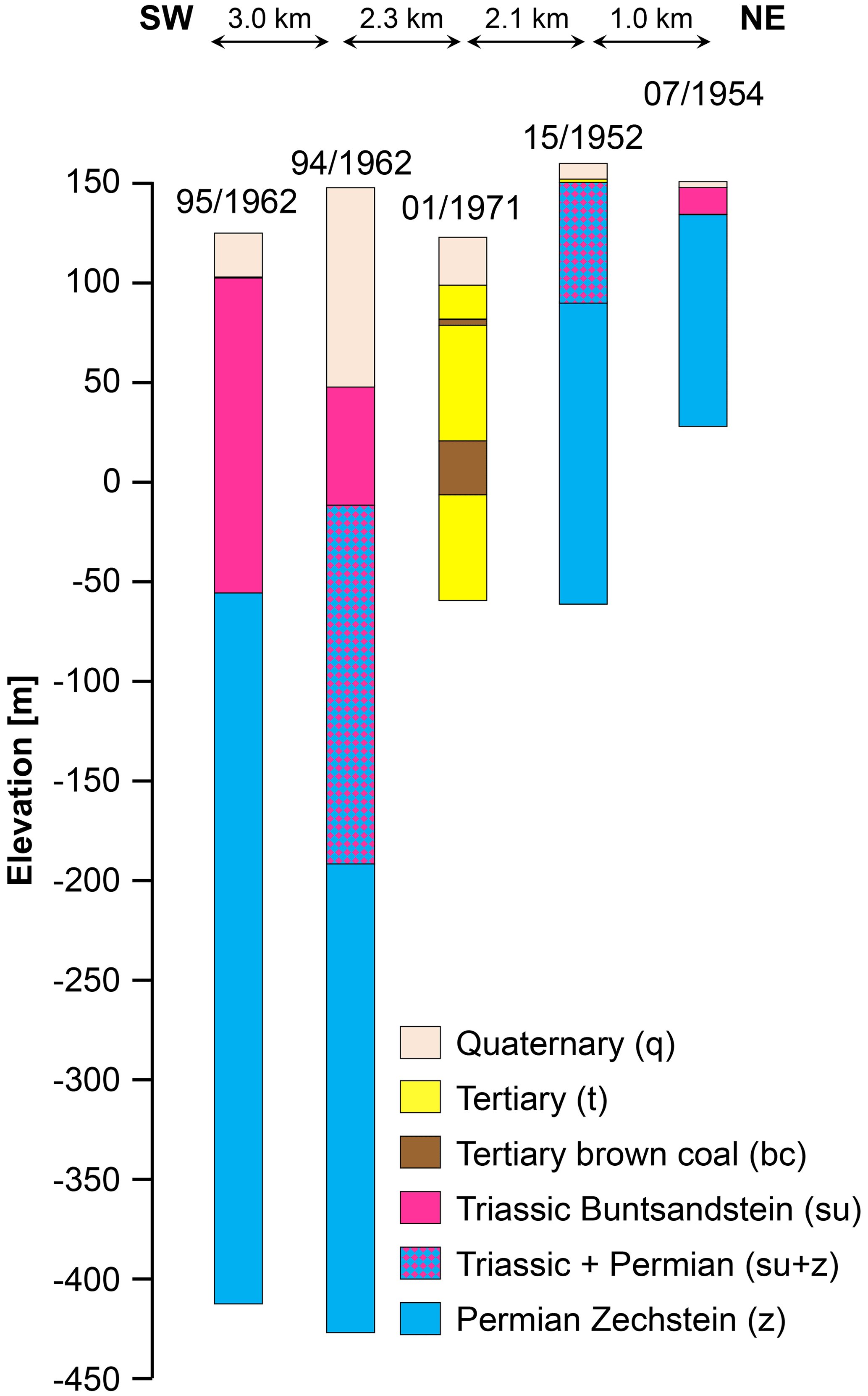
Figure 2Stratigraphy of five boreholes in and around the Esperstedter Ried. The locations can be found in Fig. 3. The stratigraphic units were used for the interpretation of the seismic profiles.
East of Bad Frankenhausen in the Esperstedter Ried, P- and SH-wave reflection seismic surveys as well as ERT, fixed-loop TEM, and gravimetric measurements were carried out along several profiles (Fig. 3).
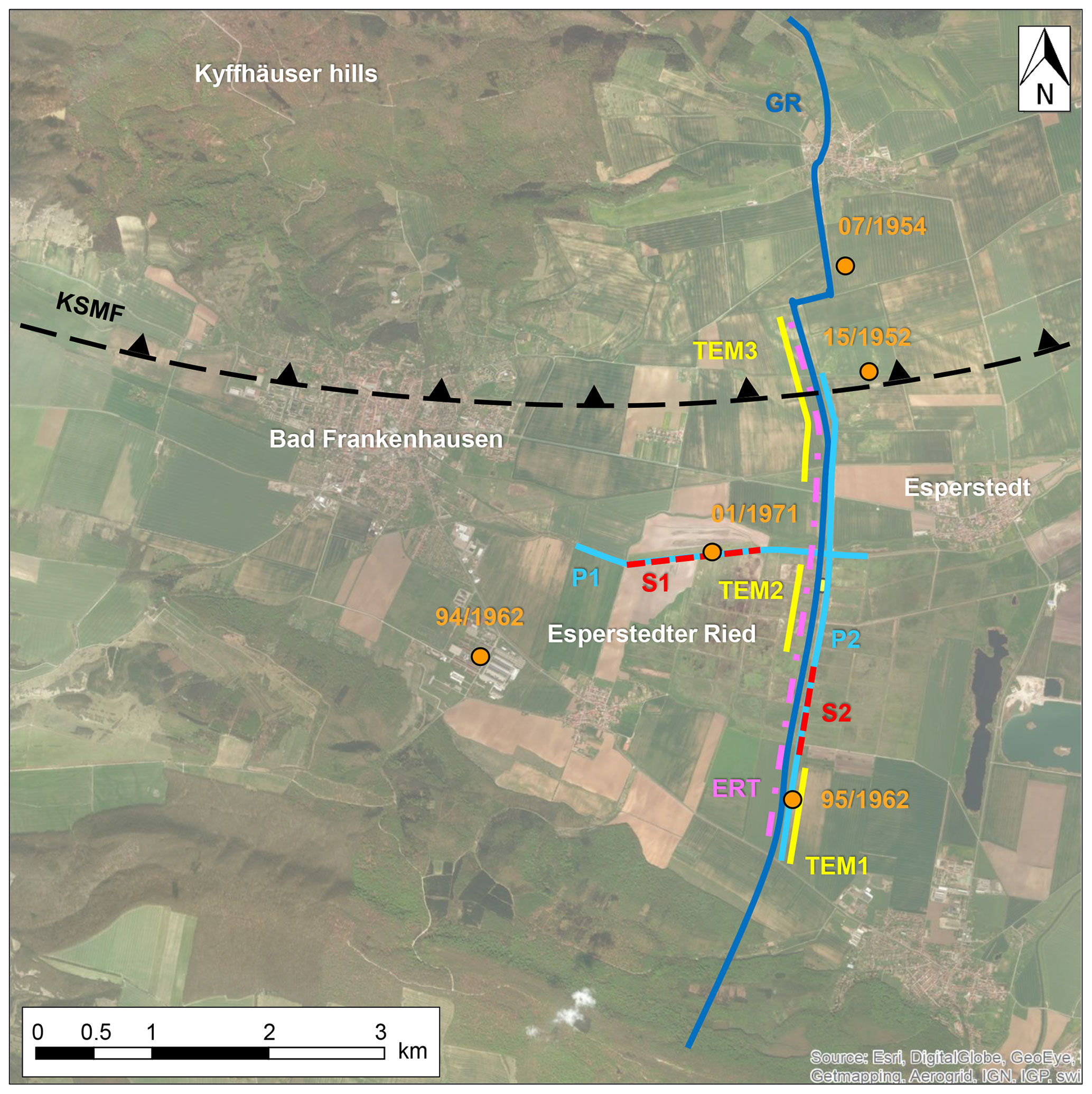
Figure 3Esri ArcGIS map showing the locations of the P-wave (light blue lines) and SH-wave (red lines) reflection seismic profiles, the gravimetric profile (dark blue line), the ERT profile (pink line), the TEM profiles (yellow lines), and the boreholes (orange dots). The thrust fault (KSMF) is marked by a dashed black line with triangles on the hanging wall.
3.1 P-wave reflection seismic
The aim of the P-wave reflection seismics was to image the large-scale geological structures to about 300 m depth. For the survey we used a 3 t hydraulically driven vibrator (HVP-30) as a seismic source, which excited compressional waves using a linear 16 s sweep from 20 to 140 Hz at 10 m spacing. At each vibrator location, three vibrations were excited. For recording we used 360 one-component vertical geophones planted in the ground at 5 m intervals (Fig. 4), resulting in an active recording line of 1800 m length. The vibrator operated in an asymmetric split-spread mode; every 360 m the line was moved forward when the vibrator reached the center of the line. This resulted in a minimum offset of 840 m for each shot and a common midpoint (CMP) fold varying between 72 and 96 traces along the line. The overall profile length was around 3 km (P1) and 5 km (P2), respectively. The data were already correlated in the field using the sweep sent by the sweep generator, and the sample rate was 2 ms with a recording length of 3 s.
3.2 SH-wave reflection seismic
The purpose of the SH-wave reflection seismics was to image the near subsurface at higher resolution compared to P waves and thus detect small-scale features associated with local geology and subsurface dissolution. In the case of water-saturated soft sediments, which are found in the Esperstedter Ried, the velocity of the SH wave is significantly slower compared to the P-wave velocity, and this results in high-resolution images of the near surface (e.g., Dasios et al., 1999; Inazaki, 2004; Malehmir, 2019). We conducted two SH-wave reflection seismic surveys that have a profile length of around 1 km (S1) and 670 m (S2), respectively. We used a hydraulically driven vibrator (MHV-4S) that excited horizontally polarized shear waves in a sweep frequency range of 10 to 80 Hz with a sweep length of 10 s and a record length of 14 s. The source spacing was 4 m, and at each vibrator location two vibrations were excited using alternating polarities. As receivers, 120 one-component horizontal geophones of type SM-6 combined in a land streamer were utilized (Fig. 4). The land streamer is adapted for near-surface reflection seismic profiling on paved or compacted ground and uses a fixed geophone spacing of 1 m. The streamer was pulled by a car that contained a Geometrics Geode recording system. A split-spread geometry was used with the source and the receivers moving forward. After surveying 60 m, the land streamer was moved 60 m forward, while the source continuously moved 4 m forward, resulting in a CMP fold of 16 to 24 traces for S1 and 32 to 48 traces for S2. The main advantage of this source–receiver combination on paved ground is the suppression of surface Love waves (Polomet al., 2010; Polom et al., 2013; Krawczyket al., 2012; Krawczyk et al., 2013).
3.3 ERT and TEM
The goal of the electrical resistivity tomography (ERT) and the transient electromagnetic (TEM) surveys was to investigate the subsurface resistivity distribution to determine zones of dissolution and areas of potential saltwater rise. Whereas the large-scale direct current measurements provide robust information about the general resistivity structure, but with comparatively poor resolution, TEM is especially suited to resolve good conductors down to a few hundred meters of depth (Milsom and Eriksen, 2011). The ERT survey was conducted with a dipole–dipole configuration using 26 pairs of electrodes with approximately 200 m spacing along the 4.5 km N–S profile. The transmitter provided up to 30 A of source current, and voltages were recorded with nine remotely controlled data loggers (Fig. 4) developed at LIAG (Oppermann and Günther, 2018).
The ERT was restricted by power lines, roads, and a gas pipe. By choosing a fixed-loop setup for the TEM survey, it was possible to cover parts of the profile that are nearly unaffected by strong artificial electromagnetic noise. Receiver positions had 50 m spacing in the N–S direction and were placed across four large transmitter loops with 250 m × 250 m dimensions. For more information about the survey and specific details of sensors and data analysis, we refer to Rochlitz et al. (2018).
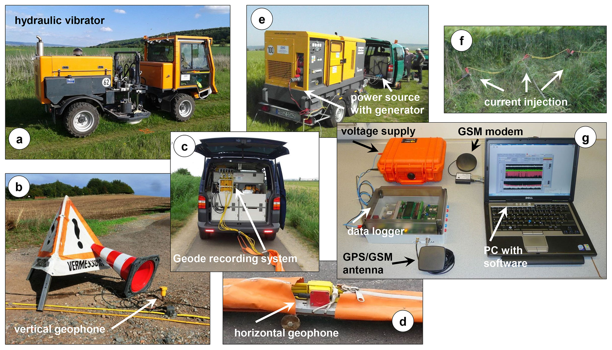
Figure 4Seismic (a–d) and ERT (e–g) equipment of LIAG used during the field campaigns. For the seismic surveys hydraulic P-wave and S-wave vibrators (a) were used as active seismic sources, and vertical and horizontal geophones (b, d) were used as receivers. A Geometrics Geode recording system (c) was also used. For the ERT surveys, a mobile power source consisting of a generator (e), electricity power inputs plugged into the ground (f), and an adapted recording system (g; photos taken from Oppermann and Günther, 2018) was utilized.
3.4 Gravimetry
The gravity survey (TLUBN, 2017) was carried out by the company Geophysik GGD mbH in 2013 on behalf of the Thuringian State Institute for Environment, Mining and Conservation (TLUBN). Its aim was to complement information from the reflection seismic surveys by imaging density contrasts in the subsurface of the Esperstedter Ried and to facilitate 2D forward modeling, where structural information from reflection seismic interpretation is available as a constraint. The focus was more on the regional basin structure than on local surface inhomogeneities. The gravity survey was carried out along a profile with a station spacing of 100 m using a Scintrex CG-5M quartz gravimeter with nominal ± 0.005 mGal standard deviation of repeated measurements. The positions and elevations were determined by differential GNSS or by total station surveys with a standard deviation of ± 0.02 m. To enable a map-based qualitative interpretation, supplementary gravity data from the regional survey of Thuringia, acquired in the second part of the 20th century, with a mean point distance of 1 to 2 km and standard deviations between ± 0.01 and ± 0.06 m Gal (Conrad, 1996) completed the dataset.
4.1 P-wave reflection seismic
The processing of the P-wave data was carried out using the processing software SeisSpace by Halliburton. The first processing steps of the P-wave data were quality control, vertical stack of three repeated shot records, geometry assignment (Fig. 5a), muting of surface waves, and application of refraction statics (Fig. 5b). This was followed by spectral balancing to improve the signal-to-noise ratio (SNR) of the reflection events and a scaling using an automatic gain control (AGC) with a 500 ms window (Fig. 5c). In preparation for the pre-stack depth migration (PSMD), short-wavelength refraction statics and residual statics were carried out, and with an interactive velocity analysis an initial velocity model was calculated. A Kirchhoff pre-stack depth migration algorithm was applied, and the velocity model was iteratively improved by residual moveout (RMO) analysis of the common reflection point (CRP) gathers. Finally, the CRPs were further processed using an additional spectral balancing, a top trace mute, and a frequency–wavenumber (F–K) filter to improve SNR and resolution (Fig. 5d). For detailed explanations of the processing algorithms, see, e.g., Hatton et al. (1986), Lavergne (1989), and Yilmaz (2001).
4.2 SH-wave reflection seismic
The processing of the SH-wave data was carried out using the processing software VISTA Version 10.028 by Gedco (now Schlumberger). At first, each record was visually examined for quality assessment, and then vibroseis correlation and geometry assignment using crooked-line binning with a 0.5 m bin interval were carried out. The next steps included amplitude balancing and frequency filtering to enhance the reflection response and to attenuate noise to improve the resolution and the data quality. For this purpose an automatic gain control (AGC, 200 ms; Fig. 5e), a bandpass filter (– Hz), and amplitude normalization were applied to the data. Then the two shot records of each vibrator location were vertically stacked to improve the SNR due to a reduction of statistically distributed noise and an amplification of the seismic response. This was followed by a top mute (Fig. 5f) and F–K filter to eliminate noise and harmonic distortions (Fig. 5g). To prepare the data for the following interactive and iterative velocity analysis, the datasets were sorted from the shot domain sort to the CMP domain sort. The manual picking of velocities was performed using semblance, offset gathers, and constant velocity stacks. With normal moveout (NMO) corrections, the reflection hyperbolas were corrected to get zero-offset travel times, and residual statics corrections reduced the inaccuracies at the near surface. A stacked seismic section in the time domain was created, and additional bandpass and F–K filters removed remaining noise. The final frequency bandwidths were – Hz for S1 and – Hz for S2. Furthermore, spectral balancing was applied, and finite-difference (FD) migration moved the dipping reflectors to their true position; finally, the sections in the time domain were converted to depth. See, e.g., Hatton et al. (1986), Lavergne (1989), and Yilmaz (2001) for detailed descriptions of the processing algorithms.
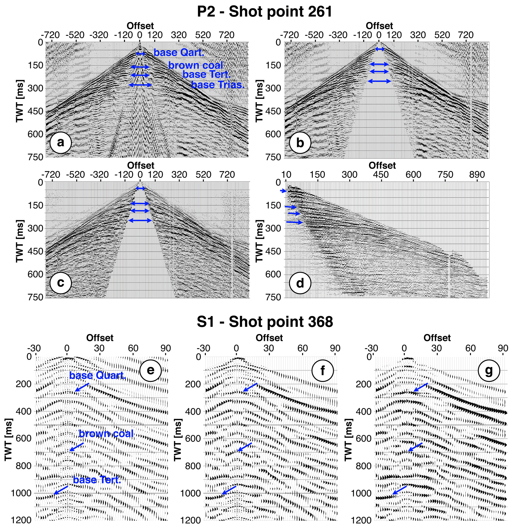
Figure 5Some of the processing steps for the P- and SH-wave reflection seismic data shown exemplarily for an individual shot record. Shot point 261 of P2 is located at around 4.68 km profile length in the final depth section shown in Fig. 7. Shown are (a) the raw data with an AGC of 500 ms, (b) the data after application of mutes and refraction statics, (c) the data after additional spectral balancing and scaling, and (d) the CRP shifted to a reference datum at the position of shot point 261 after Kirchhof PSDM. Shot point 368 of S1 is located at around 1.24 km profile length in the final depth section shown in Fig. 6. Shown are (e) the raw data with an AGC of 200 ms, (f) the data after application of a bandpass filter, a vertical stack and a top mute, and (g) the data after additional FK filtering. The blue arrows mark the base of the Quaternary, the brown coal, and the base of the Tertiary in the shot records of P2 and S1, as well as the base of the Triassic sandstones in the shot record of P2.
4.3 ERT and TEM
The ERT surveys yielded time series of 27 current injections and for each of them 26 potential difference measurements with a GPS base. The resistances were determined using a lock-in algorithm, whereby the potential difference is extracted from the noisy time series by using the known time dependence of the injected current signal (Oppermann and Günther, 2018). The apparent resistivities were calculated by multiplication of the resistance with a geometric factor, which depends on the distances between the potential and current electrodes. From these apparent resistivities a pseudo-section was created. The true resistivities were then reconstructed using the BERT inversion algorithm (Günther et al., 2006) based on a triangular model discretization that is able to take topography into account. For regularization, we used a geostatistical operator (Hermans et al., 2012; Jordi et al., 2018) with a correlation length of 800 m for the horizontal direction and 70 m for the vertical direction in order to account for the predominant layering of the geological strata.
Processing of TEM data mainly includes noise removal by selective stacking and logarithmic gating. 1D inversion of the processed data was challenging because they were affected by strong atmospheric and anthropogenic noise. The two obtained resistivity distributions based on the coil and SQUID receivers are overall similar, but the inversion results based on the SQUID receiver exhibited higher consistency between neighboring stations, greater penetration depths, and fewer artifacts caused by anthropogenic noise (Rochlitz et al., 2018). Nevertheless, using resistivity constraints from ERT and structural information from seismics, the reliability of inversion results could be evaluated.
4.4 Gravimetry
The processing of the gravity data (densely sampled stations along a profile in the Esperstedter Ried and sparse stations from regional surveys nearby) consisted of a uniform conversion of gravity observations to Bouguer anomalies. It followed the processing scheme, which was used for the preparation of the gravity database of the Leibniz Institute for Applied Geophysics in order to create a homogeneous dataset for Germany (Skiba et al., 2011). Thus, it refers to common geodetic and geophysical reference systems (ETRS89, DHHN92, and IGSN71), a standard Bouguer density of 2670 kg m−3, and a maximum radial distance of 166.70 km for the calculation of a spherical Bouguer cap and terrain effects. The formulas used comply with international standards (for details, see, e.g., Hinze et al., 2005): normal gravity by the closed-form formula of Somigliana (1929), atmospheric correction to normal gravity, free air correction by a series expansion to the second order, and a Bouguer correction by a closed formula for the gravity effect of a spherical cap of 166.70 km radius. Due to the use of ellipsoid heights for the calculation of normal gravity and geoid heights for the correction of the Bouguer cap and the terrain corrections, the resulting Bouguer anomalies contain an indirect geophysical effect. However, this is a common international simplification in the calculation of Bouguer anomalies. Furthermore, this indirect geophysical effect does not affect the results and interpretations of this study due to the local study area of only 12 km × 12 km and the rather regional trend (mainly N–S and NE–SW) of only 3.5 m Gal (in addition to a mean value of 8.6 m Gal; Skiba et al., 2011).
Spherical terrain corrections were calculated using the DEM-D with 25 m cell size that was provided by BKG (2009). Its accuracy is ± 1–4 m for the position and ± 1–5 m for the heights, the latter depending on the roughness of the topography; height resolution is 0.01 m. For areas outside Germany, the DEM-D was complemented by SRTM data. The spherical terrain corrections were calculated in two steps: step 1 considered the near-field terrain between 0 and 25 km of distance from a station using the DEM with 1 arcsec (ca. 25 m) cell size, whereas step 2 considered the far-field terrain between 25 and 166.70 km of distance using the same DEM, but the heights were interpolated to 10 arcsec (ca. 250 m) cell size. The resulting complete Bouguer anomaly is the difference between the observed gravity and the sum of all correction terms. With regard to the accuracy of the results, it can be said that even if, for example, there is a height accuracy of only 0.2 m, the maximum error that would propagate into the Bouguer anomalies (Bouguer cap and free air correction) would be only 0.4 mGal, which would not significantly influence the interpretation. The regional data surrounding the Esperstedter Ried (12 km × 12 km area) have been gridded using kriging. This grid of Bouguer anomalies was subject to spectral filtering to enhance the visibility of regional density contrasts and potential faults. Several spectral domain filters were tested in order to locate possible sources of gravity anomalies and to highlight fine changes in the gravity field. Finally, a so-called “tilt derivative” or “tilt angle” filter (Miller and Singh, 1994) was applied, which is defined as
where VDR is the first vertical derivative of the gravity anomaly, and THDR is the total horizontal derivative. This filter process generates maxima centered above the source of the anomaly. Its zero crossing is located close to the edges of source bodies. All amplitudes are restricted to values between and (+90∘ and −90∘), thus suppressing strong amplitudes and amplifying weak amplitudes.
The anomalies along the local profile in the Esperstedter Ried served as input for iterative 2.5D forward modeling. This quantitative interpretation step was realized using IGMAS+ (Interactive Geophysical Modelling Application System; Schmidt et al., 2011). This software, originally designed for 3D gravity data, gravity gradient, and magnetic modeling, enables the definition of bodies with constant or varying densities on polygonal cross sections (2D vertical planes) with finite strike length, thus enabling 2.5D forward modeling. A 2.5D model allows the rapid verification of hypotheses about the mass distribution in the subsurface in cases in which structural information is available only along profiles. As structural constraints for the upper 500 m, we used the interpreted sections of seismic profiles P2 and S2, the five shallow boreholes from the Esperstedter Ried along with their corresponding lithological information, described above, and a stratigraphic cross section included in the geological map (Schriel and Bülow, 1926a, b) extending outside the study area and incorporating other deeper boreholes further away. For the deeper part, the main constraint was the aforementioned stratigraphic cross section that runs parallel to the gravimetric profile approximately 2.5 km to the west, which was projected onto it. This cross section also enabled the implementation of a more detailed layering and a stratigraphic subdivision within the Zechstein deposits, which could not be resolved by the seismic profiles due to resolution limits. The densities used in the modeling are mean values from geophysical textbooks (e.g., Hinze et al., 2013) and from forward modeling of adjacent areas (e.g., Gabriel et al., 2001, and references therein).
5.1 Interpretation of seismic profiles P1 and S1 (W–E)
Reflection seismic profiles P1 and S1 were carried out across the Esperstedter Ried from west to east. P-wave profile P1 is 2.98 km in length, and SH-wave profile S1 is 1.04 km in length. Profile S1 was surveyed after P1 and covers a selected area based on the interpretation of P1, which shows interesting near-surface structures in the western part.
In P1 and S1 (Fig. 6a, d) from the surface down to ca. 100 m depth and between ca. 1.20 and 1.50 km profile length, mostly horizontal and continuous reflectors with partly high amplitudes are imaged, which represent Quaternary and Tertiary deposits (Fig. 6). These impedance contrasts represent layer boundaries. The high-amplitude reflector at ca. 10 to 25 m depth, which is visible in both sections and traceable throughout the entire profile of S1, represents the boundary between the Quaternary gravel and silt and the Tertiary clay. In section P1 (Fig. 6a), at about 100 m depth within the Tertiary deposits, another high-amplitude reflector is imaged. It is mostly continuous and traceable throughout the entire profile, which we interpret as Tertiary brown coal and use as a marker horizon (Fig. 6b). In S1 (Fig. 6d), the brown coal shows no distinct reflector, but instead the internal structures of the Quaternary and Tertiary deposits can be observed in more detail compared to the P-wave section (for details see Sect. 5.3 and Fig. 8). Below the top Triassic, at ca. 250 m depth in P1, a horizontal reflector showing a partly strong impedance contrast is imaged in the east of both sections between 1 and 2.40 km profile length, especially in P1 (Fig. 6a, b). This is interpreted as the boundary between the Lower Triassic sandstones and the Permian evaporites. The sandstones of the Lower Triassic show almost no internal structures, and the area below the top of the Permian contains only poor reflections, probably due to the limited penetration depth of the seismic waves and the resolution limits.
To the west of P1 and S1, between 0 and ca. 0.75 km profile length, shallowly dipping reflectors form a bowl-shaped structure ca. 0.70 km in length at 100 to 300 m depth within the Tertiary, Triassic, and Permian deposits (Fig. 6a, c, d). The brown coal marker horizon was used to support the interpretation, since no boreholes are available in this area. Profile S1 shows only the eastern margin of this structure, but it gives more detailed information on the internal features of the formations with respect to the P-wave profile (Fig. 6d, e). Onlapping silt and clay layers of the Tertiary are observed above the coal, and further above are horizontal Tertiary and Quaternary deposits. Between ca. 0.80 and 0.90 km profile length at ca. 100 to 280 m depth V-shaped reflectors are observed in P1 (Fig. 6c). The same zone is characterized by synclinal reflectors and low reflectivity in S1 (Fig. 6d).
The Triassic sediments show local thinning and a general decrease in thickness from east to west. Numerous faults and fractures in the Tertiary, Triassic, and Permian formations are imaged (Fig. 6f). In P1 steeply dipping normal and reverse faults, which transverse the seismic profile, are identified, and in S1 not only the faults of P1 are imaged, but also other steep faults and many nearly vertical fractures within the bowl-shaped structures, some of which have been drawn in the interpretation (Fig. 6). These are not be observed in P1 since their scale is below the resolution limit of the P-wave profiles (Fig. 6e).
We interpret the large bowl-shaped structure (Fig. 6b, e, f) to be a former collapse sinkhole that opened during the Tertiary. The nearly vertical fractures within and below the subsidence sinkhole that crosscut the Triassic and the Permian indicate collapse of an underground cavity. Since the brown coal layer dips and is crosscut by some of the fractures, the sinkhole must have occurred after the deposition of the organic material. This is supported by the onlapping Tertiary and the horizontally layered Quaternary sand and gravel above. The small structure more to the east seems to be a second collapse sinkhole with steep margins (Fig. 6e, f).

Figure 6Seismic profiles P1 and S1 uninterpreted (a, c, d), with interpreted stratigraphy (b, e), and combined interpretation with seismic facies and seismic features (f). The red box in (a) marks the detail of P1 in (c) and the position of the SH-wave profile shown in (d) and (e). The seismic facies (A–F) and the seismic features (SF1–SF2) are exemplarily marked and are explained in Sect. 5.3 and Fig. 8. The vertical exaggeration is 2:1, and the reference datum is 126 m a.s.l. for P1 and 124 m a.s.l. for S1.
5.2 Interpretation of seismic profiles P2 and S2 (S–N)
Reflection seismic profiles P2 and S2 were carried out from south to north. P-wave profile P2 is 5.10 km in length, but only the first 4.50 km is analyzed because of poor reflectivity in the most northern part. The SH-wave profile S1 is 0.67 km in length. Profile S2 was surveyed after P2 and covers a selected area based on the interpretation of P2, which shows interesting near-surface structures in this part of the profile. The profile lengths of P2 and S2 were adapted so that they match the gravimetric profile to enable better comparability of interpretations; thus, e.g., P2 starts at 2.10 km and ends at 6.60 km.
The most northern part of P2 between ca. 6.35 and 6.60 km profile length from the surface down to about 400 m depth (Fig. 7a, b) shows irregular and discontinuous reflectors of low amplitudes. They represent the Permian Zechstein formations of the Kyffhäuser hills. This area is separated from the south by a steep, northward-dipping thrust fault, the KSMF.
South of the KSMF, at 50 to 100 m depth (Fig. 7a, b), a continuous, high-amplitude reflector is imaged, which is traceable throughout almost the entire profile. Just as in P1 and S1, this impedance contrast is interpreted as the boundary between the Quaternary and Tertiary deposits. A second, mostly continuous reflector with high impedance contrast is visible between ca. 2.90 and 6.35 km profile length at 100 to 200 m depth, which is interpreted as the top of the brown coal (Fig. 7a, b, d, e) and is further used as a marker horizon. The thickness of the Tertiary formation decreases from north to south. The Triassic sandstones below show no internal structures, but at ca. 250 m depth, a discontinuous, high-amplitude reflector is imaged. This is interpreted as the top of the Permian Zechstein, which is traceable throughout the entire profile P2 (Fig. 7a, b). Repeatedly, between 3.20 and 6.35 km profile length the reflector shows low reflectivity, but between ca. 2.40 and 3.20 km profile length it is continuous and has even higher amplitudes. These two areas are separated by a steep northward-dipping normal fault (Fig. 7b, e, f).
Directly south of the KSMF, between 5.10 and 6.35 km profile length, dipping reflectors that form a bowl-shaped structure within the Quaternary to Permian deposits are imaged (Fig. 7a, b, f). In contrast to the two structures observed in P1 and S1, the Quaternary is affected too. The deepest point of the bowl-shaped structure is at ca. 400 m depth and coincides with a low-reflectivity zone in the Permian Zechstein. Another 0.30 km wide depression was identified to the south between 2.10 and 2.40 km profile length at 200 to 350 m depth within the Quaternary to Permian sediments (Fig. 7a, b). A third bowl-shaped structure was imaged at shallow depth in the near surface between 3.30 and 3.45 km profile length at ca. 40 to 100 m depth. This was pointed out as the area of interest for the SH-wave reflection seismic survey S2 (Fig. 7c, d, e). The high-amplitude reflectors of the top of the Tertiary are also observed in S2, but the impedance contrast is weaker than in P2. In S2 details of the internal structure of the different formations can be recognized (for details, see Sect. 5.3 and Fig. 8).
Besides the KSMF, other steep faults are identified below the northern depression and below the near-surface structure to the south (Fig. 7f). Profiles P2 and S2 reveal that the fault below the near-surface structure, between 3.30 and 3.45 km profile length at ca. 40 to 100 m depth, is not a single fault but is instead a fault zone, and nearly vertical fractures within the lower Tertiary sediments are also imaged in S2.
The low-reflectivity areas of the top Permian are assumed to be the result of leaching and dissolution processes, similar to the bowl-shaped structures, which are interpreted as a near-surface collapse sinkhole that developed due to cavity collapse and two deep, syn-sedimentary, sagging sinkholes that were generated due to slow mass movement of material. In contrast to the dissolved Permian to the north, it is less affected by dissolution to the south, as indicated by strong impedance contrasts, which are probably the result of unimpaired evaporite sequences. The steep fault, at ca. 3.20 km profile length, may serve as a barrier for groundwater flow coming from the Kyffhäuser hills.

Figure 7Seismic profiles P2 and S2 uninterpreted (a, c, d), with interpreted stratigraphy (b, e), and combined interpretation with seismic facies and seismic features (f). The profile lengths of P2 and S2 were adapted so that they match the gravimetric profile to enable better comparability of interpretations; thus, e.g., P2 starts at 2.10 km and ends at 6.60 km. The red box in (a) marks the detail of P2 in (c) and the position of the SH-wave profile shown in (d) and (e). The seismic facies (A–F) and the seismic features (SF1–SF4) are exemplarily marked and are explained in Sect. 5.3 and Fig. 8. Borehole 01/1971 was projected onto the seismic profile over a distance of 1 km; borehole 15/1952 was projected over a distance of 430 m, and borehole 95/1962 is located directly beside the seismic section. The vertical exaggeration of the seismic sections is 2:1, and the reference is 150 m a.s.l. for P2 and 121 m a.s.l. for S2.
5.3 Seismic facies analysis
The procedure of the seismic facies analysis is based on Roksandic (1978). A total of six seismic facies types (A–F) and four seismic features (SF1–SF4) can be identified in the P- and the SH-wave seismic data on the basis of configuration, continuity, amplitude, and frequency content (Fig. 8). A comparison of P-wave and S-wave data was not possible for all facies and feature types because for some locations only P-wave data were available.
The three facies A–C are characterized by continuous to semi-continuous reflectors and represent more or less undisturbed layers. Facies A consists of Quaternary and Upper Tertiary with continuous, horizontal, and parallel reflectors. Compared to the S-wave sections, the P-wave sections show low amplitudes in the uppermost part due to resolution limits. As a result, the silt, sand, and gravel layers of the Quaternary are not imaged, and the deeper parts are of high amplitudes. The S-wave data, however, show generally high amplitudes with a high-frequency content, and the differentiation of individual reflectors within the two formations is more detailed due to the improved resolution. Facies A might be a good water conduit for horizontal water flow due to the permeable gravel and sand layers, but noticeable vertical fluid pathways, which are important for subsurface dissolution, were not identified. Facies B shows the internal structures of the lower Tertiary silt, gravel, sand, and clay, and it has semi-continuous, wavy to sigmoid-parallel reflector patterns. Both P- and S-wave data show a high-frequency content, but the amplitudes in the S wave are higher for this facies, and the reflectors are thinner and more detailed compared to the P-wave data. Facies B, with its semi-continuous reflector patterns, could favor vertical water flow. Facies C shows the Tertiary fill of a dissolution-induced sinkhole with oblique to parallel reflectors. P-wave and S-wave data show slightly different images. In the P-wave data, the Tertiary fill is visible as semi-continuous reflectors of medium amplitudes and medium-frequency content, and in the S-wave data an onlap fill is observed with continuous reflectors, high amplitudes, and medium-frequency content. In contrast to the Tertiary deposits of facies B, the depression fill does not seem to be strongly fractured.
The three facies D–F are characterized by mostly discontinuous reflectors and represent disturbed layers. Facies D consists of Lower Triassic sandstones of the Buntsandstein, and the pattern configuration can be described as hummocky clinoforms. In the P-wave data this facies is discontinuous, is of low amplitudes, and has low-frequency content, and in the S-wave data semi-continuous reflectors of medium amplitudes and medium frequencies are observed. The sandstones are disturbed and no internal structures are identified for both wave types; as a result, it is most likely that the fractured, permeable sandstones serve as fluid pathways for vertical and lateral groundwater flow. Facies E shows the different types of the top Permian horizon, which are identified in the seismic sections. Facies E1 shows the undisturbed case with continuous, mostly horizontal, and parallel reflector patterns. Two differentiations for the undisturbed evaporite can be made. High amplitudes might indicate thicker salt layers that generate a stronger impedance contrast against the Triassic sandstones above compared to medium amplitudes of possibly evaporite (anhydrite, gypsum) that would generate a weaker impedance contrast. Facies E2 shows the disturbed case with discontinuous, hummocky to chaotic reflection patterns, low amplitudes, and low-frequency content. Both P-and S-wave data show the same characteristics, and this facies is interpreted as fractured and leached Zechstein formations, as well as potential zones affected by dissolution processes. Facies F images the interior of the Permian Zechstein formations. Just like for facies E2, P- and S-wave data are very similar, showing discontinuous and chaotic reflectors with no internal structures.
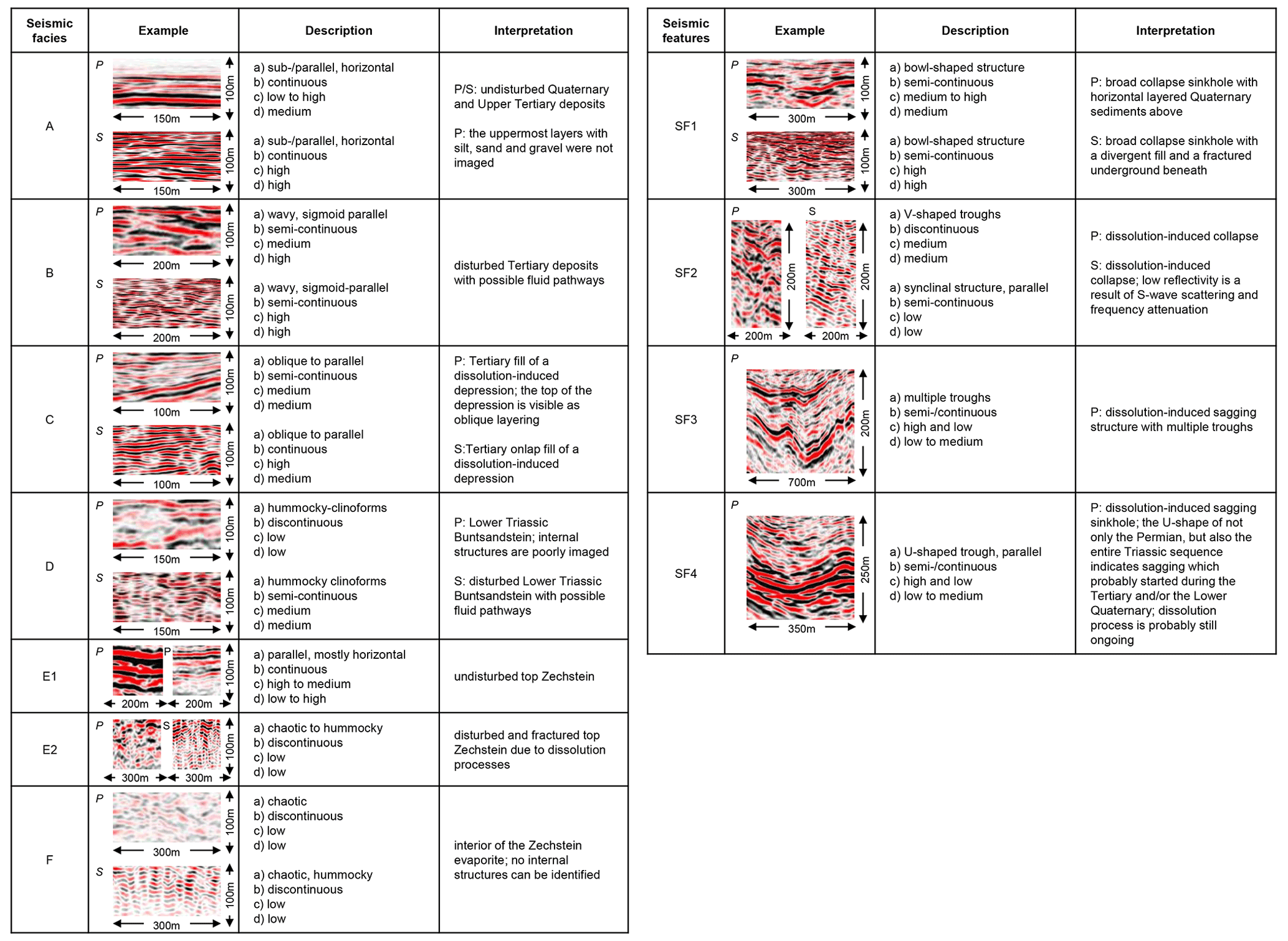
Figure 8Six different seismic facies (A–F) and four seismic features (SF1–SF4) were identified in the study area. Four seismic reflection parameters were used to classify the different types: (a) configuration, (b) continuity, (c) amplitude, and (d) frequency. The P-wave and S-wave facies are marked with “P” and “S”. Comparison of P- and SH-wave data could not be carried out for all facies and feature types because for some locations only P-wave data are available.
Seismic feature SF1 consists of semi-continuous reflector patterns that form a bowl-shaped structure in both P- and SH-wave data, although the amplitudes in the SH-wave data are generally higher, as is the frequency content. It is interpreted as a broad collapse sinkhole with more or less horizontal layers above. In the S-wave data a divergent fill and fractured rocks beneath the sinkhole are identified. Seismic feature SF2 shows different characteristics in P waves and S waves. In the P-wave data, discontinuous reflectors form V-shaped troughs of medium amplitudes and medium-frequency content, whereas in the SH-wave data semi-continuous reflectors form parallel, synclinal structures of low amplitudes and low frequency. It is interpreted as another dissolution-induced, steeper collapse sinkhole. Seismic feature SF3 consists of multiple troughs of continuous to semi-continuous reflectors of high and low amplitudes and medium- to low-frequency content. It is interpreted as a dissolution-induced depression, also called a sagging sinkhole, and the sagging is either still ongoing or was active until recent times, which is supported by the fact that all formations from the Permian to the Quaternary are involved. Seismic feature SF4 is similar to SF3, but in contrast only a U-shaped trough is observed in SF4. Just like SF3 all formations from the Permian to the Quaternary are affected, which is interpreted as a sagging sinkhole, where sagging is ongoing.
Although P- and SH-wave reflection seismic data image the same subsurface structures, the seismic facies imaging can be different due to the variations in penetration depth and resolution of the seismic waves types, which can influence the interpretation of the reflection pattern. Therefore, we suggest a combined analysis of P-wave and SH-wave seismic data.
5.4 Interpretation of ERT and TEM
Figure 9 shows the inversion results of TEM and ERT in combination with the interpreted geological structures of seismic profile P2. The target depth of the TEM method is between 300 and 600 m, depending on the subsurface conductivity characteristics (Rochlitz et al., 2018), and the target depth of the ERT is ca. 400 m. For the TEM survey at fixed-loop positions 2 and 3, a five-layer model instead of the original four-layer model by Rochlitz et al. (2018) was evaluated to be more suitable to explain data as well as subsurface resistivities. The profile length annotations were adapted to match the gravimetric profile to enable better comparability of interpretations, and thus, e.g., the ERT profile starts at 2.10 km and ends at 6.60 km.

Figure 9TEM profiles (a) on seismic profile P2 and the ERT profile (b) with interpreted seismic structures in black. The profile lengths were adapted so that they match the gravimetric profile to enable better comparability of interpretations; thus, e.g., the ERT profile starts at 2.1 km and ends at 6.6 km. The vertical exaggeration is around 2:1, and the reference datum is 150 m a.s.l. for the ERT and TEM data.
In the near surface within the Quaternary deposits the electrical resistivity ranges from ca. 10 to 40 Ω m between 2.10 and 5.80 km profile length down to 30 m depth. In the north, the KSMF is located, and due to the thrust fault, leached Zechstein is found only a few meters below the surface, showing resistivities of several hundred Ω m. North of the KSMF, the salt is completely dissolved and/or eroded.
Below ca. 100 and 300 m depth a broad zone of low resistivity with less than 10 Ω m between 2.30 and 6.10 km profile length is observed. This zone corresponds to Tertiary and Triassic deposits, as interpreted in seismic sections P2 and S2. Within this zone is an extremely conductive thin layer of approximately 1 Ω m, which is particularly resolved by the TEM data. The boundaries of this layer coincide well with main seismic reflectors. It is interpreted to match saline aquifers between the lignite and the Triassic Buntsandstein. Unfortunately, there are no continuous TEM soundings across the entire profile available. In contrast, the ERT inversion data smear this layer over greater thickness due to limitations of resolution but prove its continuity.
From 3.10 to 2.10 km profile length the extremely conductive layer vanishes and resistivities between 100 and 300 m depth increase slightly, as shown by the ERT and TEM FL 1, which is probably related to the fault zone at 3.20 km. The fault might hamper the lateral groundwater flow and therefore the lateral distribution of the saltwater coming from the dissolved Permian deposits, which migrated upward along the faults and fractures to the north due to artesian-confined groundwater conditions.
The top Permian at 250 to 300 m depth, as indicated by seismic interpretation, correlates with the top of the TEM basement layer with high resistivities of more than 100 Ω m. This is also visible in the ERT result, but the contrast is smoother and does not reveal a unique basement depth. At 5.50 km profile length, the ERT shows lower electrical resistivities reaching depths of 500 m. This coincides well with the interpreted fault. This area also correlates with the position of dissolution-induced structures, like the sinkholes above. Therefore, it is an indicator for saltwater rise due to dissolution of Zechstein evaporites and artesian-confined groundwater conditions. The rising saltwater is the reason for the development of the inland salt marsh. A similar low-resistivity area at such great depths is located at 2.10 to 2.50 km on the profile. However, since the profile ends there, detailed interpretation is speculative.
Overall, the ERT and TEM results are in very good agreement with the seismic interpretation, although no joint inversion was carried out, which would improve the quality of the datasets and their interpretation.
5.5 Interpretation of gravimetry
The prominent features on the Bouguer map (Fig. 10a) are in remarkably good agreement with the near-surface strata on the geological map (Fig. 1). The contours of the central positive Bouguer anomaly of +18 m Gal (1 Gal = 0.01 m s−2) clearly follow the outline of the Carboniferous (Kyffhäuser formation) and Permian (Zechstein) rocks. The roundish negative anomaly of −8 mGal to the SW correlates with outcropping Triassic (Muschelkalk) formations, whereas the WNW–ESE strike direction of an elongated, central gradient zone matches the geometry of Tertiary and Quaternary sediments in the Esperstedter Ried.
The tilt-angle filter (Fig. 10b) reveals an elongated source beneath the Kyffhäuser hills and a local low in the southern part of the Esperstedter Ried. In general, negative values correlate well with the location of Quaternary fluvial sediments of low density and areas with presumed mass loss due to dissolution of soluble rocks, while the majority of positive values surround Triassic, Permian, and Carboniferous outcrops.
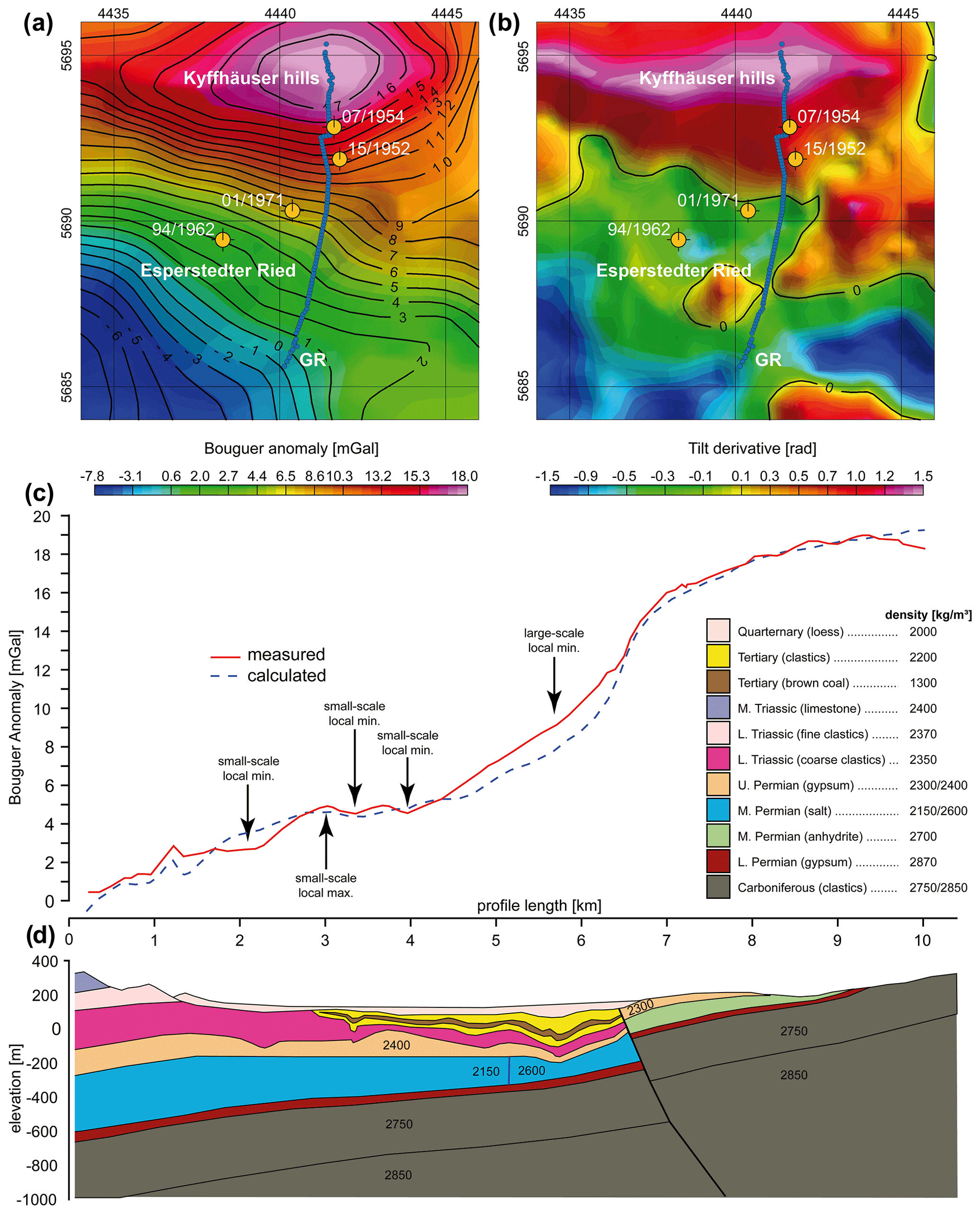
Figure 10Bouguer anomalies (a) show a positive anomaly for the Kyffhäuser hills, and the tilt derivative (b; e.g., Miller and Singh, 1994) shows a negative anomaly for the Esperstedter Ried because of mass movement due to subsurface dissolution and the accumulation of, e.g., Quaternary sediments with lower density. In the local Bouguer anomalies of the profile GR (c) three small-scale local minima and one large-scale local minimum are observed (d), which correlate with dissolution-induced mass loss identified in seismic sections P2 and S2. The legend contains the description of the modeled formations and their assumed densities taken from the literature. The blue line in (a) and (b) is the gravimetric profile GR. The vertical exaggeration is 2:1.
Quantitative interpretation was accomplished by iterative 2.5D forward modeling of the gravimetric profile GR (Fig. 10c, d). This simplified approach is suitable for the S–N profile, since the Bouguer anomalies depict an elongated structure of roughly 10 km length. It strikes nearly perpendicular to the profile and therefore exhibits, as a first-order approximation, a 2D character. The measured anomalies (red curve in Fig. 10c) show a strong positive anomaly of +18 mGal in the northern part of the profile and decreasing values towards the south, reaching a minimum of 0.4 mGal. Three small-scale (short wavelength) minima and one large-scale (long wavelength) minimum are observed in the southern part. The large-scale positive anomaly in the north results from the uplifted Kyffhäuser hills and the KSMF, a reverse fault, which is represented by high-density Permian and Carboniferous strata and the absence of low-density rock salt in this region. The Kyffhäuser hills have only a thin cover of unconsolidated material but consist of dense bedrock (e.g., conglomerate, anhydrite) close to the surface. The generally lower Bouguer values in the southern part result from a thicker cover of unconsolidated sediments, damage zones within the bedrock as observed in the seismic sections, the presence of low-density material, especially Tertiary brown coal and Permian salt, and possible formation of open or filled cavities. The latter is interpreted as a result of the dissolution processes at ca. 300 m depth. South of the KSMF, three local small-scale minima are identified (Fig. 10c and d), which are not well explained by the modeling approach (blue curve in Fig. 10c) using constant densities for each layer. These minima correlate with dissolution-induced sagging and collapse sinkholes imaged on the corresponding seismic profiles P2 and S2 (Fig. 7). Therefore, locally varying densities are plausible; e.g., the Permian Zechstein of an area that is strongly affected by dissolution has a higher density (2600 kg m−3) than in areas with fewer or no dissolution processes (2150 kg m−3) due to the absence of salt, which has a low density (see, e.g., Müller et al., 2021). Furthermore, between the two southernmost local minima (at ca. 3 km profile length), a weak positive local maximum is detected, which correlates with a high-amplitude reflector of the top Permian in seismic profile P2. This indicates less or no dissolution in this area compared to the northern part of the Esperstedter Ried. The observed misfit in the forward modeling, e.g., the difference between measured and calculated anomalies, suggests that locally limited areas with varying densities must be located at depths of, e.g., 150 m to 250 m. Further to the north of the inland salt marsh one large-scale minimum is observed, which correlates with a basin-like structure identified in seismic section P2 (Fig. 7). Based on our results, we assume that it developed because of syn-sedimentary sagging due to slow dissolution-induced mass movement. The syn-sedimentary development enabled the accumulation of higher quantities of unconsolidated Quaternary sediments and also Tertiary deposits with lower densities compared to the surrounding areas. As a result, a large-scale minimum is seen in the gravity data at this location.
The results show that even large-scale gravimetry can help to identify possible areas prone to dissolution and eventually sinkhole development.
6.1 Conceptual subsurface dissolution model of the Esperstedter Ried
To better understand the local dissolution processes of the Esperstedter Ried, the geological evolution of the region has to be first reconstructed. This includes the sedimentary depositional history and the development of large-scale geological structures, like faults or basins (McCann and Saintot, 2003), which can be identified directly using seismic methods and indirectly using gravimetric methods (Conrad, 1996; Hinze et al., 2013). These structures can have an influence on past and recent dissolution processes, e.g., enhanced dissolution and mass movement at faults (Closson and Abou Karaki, 2009; Del Prete et al., 2010; Ezersky and Frumkin, 2013a; Wadas et al., 2017). After reconstructing the general geological evolution of the Esperstedter Ried, the factors controlling the local dissolution processes will be outlined and a conceptual model will be presented.
In the Esperstedter Ried the P- and SH-wave reflection seismics and the gravimetric investigation revealed large- and small-scale structures, like faults, fractures, and thickness variations, delivering a structural model of the area. With regard to the fault development, it is known that from the Upper Cretaceous to the lower Tertiary that the Kyffhäuser hills were upthrusted and the KSMF developed (Freyberg, 1923; Seidel, 2003). This fault has a Hercynian strike, which can be observed in the geological map of Bad Frankenhausen (Schriel and Bülow, 1926a, b) and in the gravimetry data (Fig. 10). This preferred Hercynian strike direction of northern Germany can also be observed in the formations shown in reflection seismic profiles P2 and S2 (Fig. 7), in which other faults were identified that transverse the profiles, cut the lower Tertiary, and show approximately a NW–SE strike. It has to be noted that the Bouguer anomaly maps shown in this study have a resolution limit of 1 km and therefore cannot image this scale of faulting.
Furthermore, we assume that the uplift of the Kyffhäuser hills led to flexural isostasy (Watts, 2001) in the southern foreland and therefore regional, large-scale subsidence, which has to be distinguished from the local dissolution-induced subsidence. After Weber (1930) and also according to recent sinkhole classification models by, e.g., Gutiérrez et al. (2014) and Parise (2019), dissolution-induced sagging or subsidence can be subdivided into three phases: (1) dissolution of salt, (2) hydration of anhydrite and transformation into gypsum, and (3) leaching of gypsum. During the first phase, planar cavities are formed along the salt layer, resulting in local sagging; during the third phase funnel-shaped cavities are formed, and after collapse they form a sinkhole. These three phases can be identified in the Esperstedter Ried utilizing the seismic sections (Figs. 6 and 7) and the gravimetric modeling results. They enabled the identification of large sagging structures, e.g., visible by thickness variations (explained in more detail below) and saltwater rise that represent the first phase, as well as mass movement and collapse structures that represent the third phase. These structures can be correlated with local minima of the Bouguer anomaly (Fig. 10), which is evidence of mass movement and mass removal. Altogether this proves the assumption of dissolution-induced subsidence at the Esperstedter Ried.
Overall, the Permian, Triassic, and Tertiary formations show thickness variations across the study area. Except for local variations, a general decrease in thickness from south to north, towards the KSMF, is observed for the Permian and Triassic deposits. The thickness variation of the Triassic is probably a result of erosion after deposition and a varying accommodation space during deposition, but the thickness variations of the Zechstein are mostly the result of dissolution. Since faults are able to enhance such processes (Closson and Abou Karaki, 2009; Del Prete et al., 2010; Ezersky and Frumkin, 2013a; Wadas et al., 2017), the dissolution process is more intense close to the KSMF, and more salt and gypsum are dissolved, leading to mass movement and a decrease in thickness of the Zechstein formation. Other reasons, such as active diapirs and salt movement, for the Zechstein thickness variations can be excluded. According to the geological map, the top Carboniferous is found at ca. 550 m depth, and the thickness of the Permian is expected to be between ca. 350 and 400 m. The salt in the Permian deposits needs to be much thinner, so even if the top Carboniferous varies in depth it is highly unlikely that the salt layer would be thick enough to form active diapirs (Schultz-Ela et al., 1993; Jackson et al., 1994). Salt movement due to increased differentiated load is also unlikely because areas with a thicker Triassic Buntsandstein do not correlate with areas of thinner Permian deposits (Schultz-Ela et al., 1993); instead, the opposite is observed. However, the thickness of the Triassic sandstones does have an influence on the formation of dissolution-induced structures. Great thicknesses of a compact rock are relatively stable against subsidence and collapse because even when cavities are formed in the Zechstein formations beneath, the sediments above the cavity would form a structural arch (Waltham et al., 2005), which should prevent collapse and subsidence, whereas low thicknesses of the Triassic sandstones increase the possibility of cavity collapse and local subsidence, which is the case in the Esperstedter Ried. Further evidence for the long-lasting subsidence is given by the Tertiary brown coal that was deposited during the Oligocene and which shows a varying thickness and a dip variation of 10 to 60∘ (Frank, 1845). It is unlikely that the brown coal was deposited with such a high dip, so we assume that the brown coal thickness variations are a result of continued dissolution-induced sagging during deposition, with thinner brown coal at the basin margins and thicker brown coal at the basin center.
A better understanding of the recent local dissolution processes, however, also requires detailed knowledge about the fluid pathways and the localization of dissolution zones. This was accomplished using ERT and TEM, as well as seismic facies analysis of P and SH waves. The top of the soluble Permian rocks was detected at 250 to 300 m depth, so near-surface dissolution, as is the case for the town of Bad Frankenhausen north of the KSMF (Wadas et al., 2016; Kobe et al., 2019), is not possible. The unsaturated groundwater needs to reach greater depths in order to leach the evaporites such as salt and anhydrite. One of these groundwater levels is detected at 150 to 200 m depth according to the TEM data, which show a low-resistivity zone at this depth. Regarding this, downward water flow through a fracture network is required for its enlargement and further solution of soluble rocks (Billi et al., 2007). Although this process takes place mostly at shallower depths, a correlation between fractures and dissolution features is observed for the Esperstedter Ried from the seismic facies analysis. The low-resistivity zone of the TEM data is connected with the soluble rocks through a fractured seismic facies of the Triassic and lower Tertiary, as shown in the SH-wave data (Fig. 8). Faults are also very important for vertical water flow, and this is shown by the ERT data. At faults the water can migrate downwards and dissolve the deeper soluble rocks, as observed in seismic profile P2 and the ERT (Figs. 7 and 9), where below the sagging structures steep faults crosscut the Tertiary, Triassic, and probably Permian deposits and serve as large fluid pathways. The water can also migrate upward along the fault planes (Legrand and Stringfield, 1973) and fractures (Pusch et al., 1997; Westhus et al., 1997), mostly due to artesian-confined groundwater flow towards the surface, as is the case for the Esperstedter Ried. The ERT identified an area of low resistivity at the surface between 3.9 and 4.7 km profile length, which is the center of the inland salt marsh (Fig. 9). Besides the fluid pathways, possible dissolution zones have also been identified by the P-wave reflection seismic profiles and the ERT. Areas affected by dissolution show a less pronounced top Zechstein reflector and a lower resistivity. The leaching and mass movement destroy the layer boundary and the layering of the Zechstein, and therefore no continuous reflector can be observed (e.g., below the large sagging structure to the north of P2). The opposite is visible in the south of P2, where a strong impedance contrast without a low-resistivity zone is imaged for the top Zechstein, indicating less dissolution.
Altogether, the tectonic and depositional history indicates that dissolution processes were probably triggered by tectonic movements and fault development, and therefore they were probably most active during and after the tectonic phases of the Tertiary but are still ongoing, as evidenced by continuous saltwater rise at the Esperstedter Ried (TMLNU, 2008) as well as recent subsidence and sinkhole development (Jankowski, 1964; Wadas et al., 2016; Kobe et al., 2019).
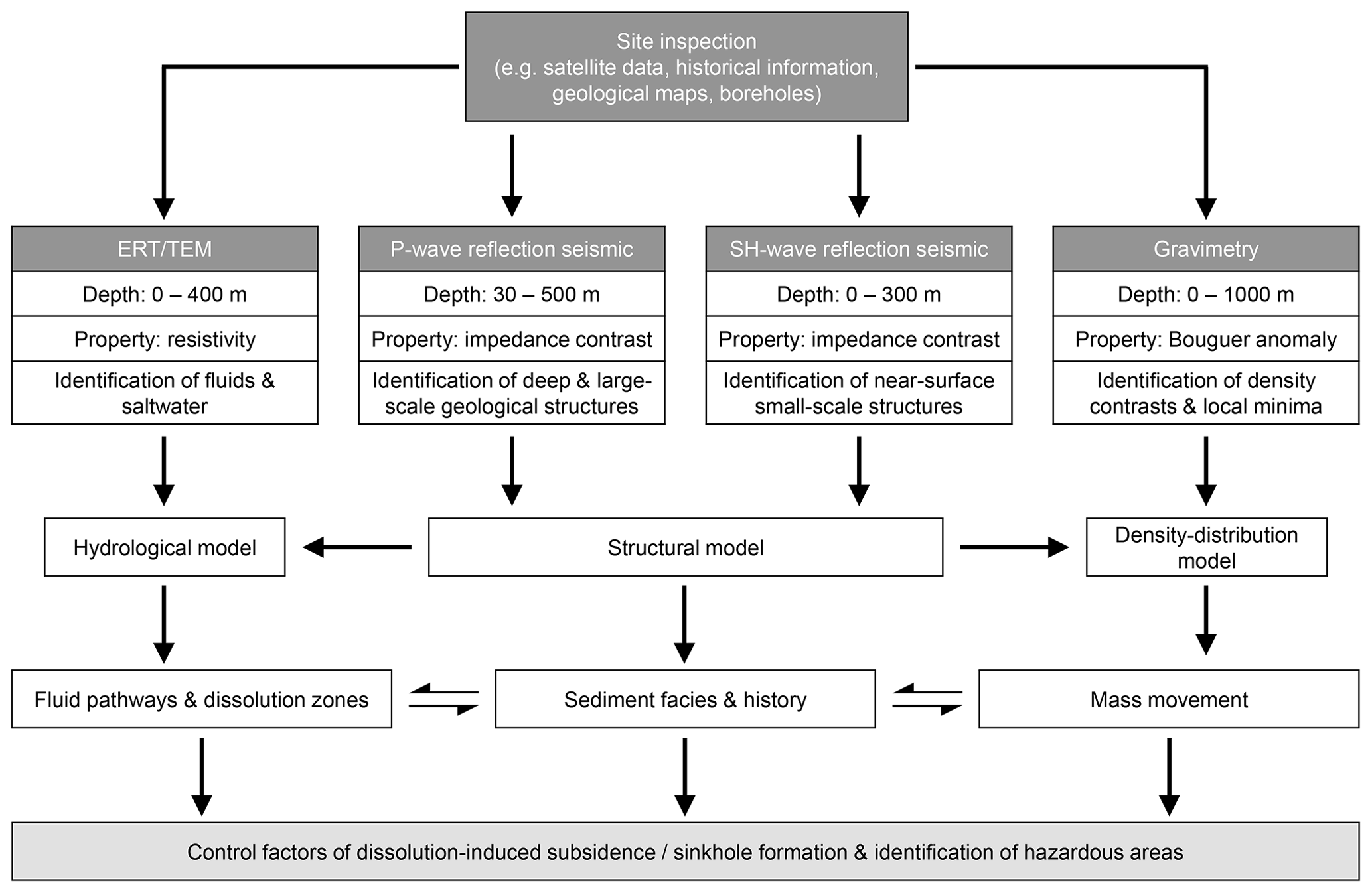
Figure 11Recommended workflow for geophysical investigations of areas prone to subsurface dissolution and sinkhole development to determine controlling factors and hazardous areas.
6.2 Workflow for geophysical investigations of areas affected by sinkhole problems
Based on the results of this study, we propose that our combined geophysical approach is suitable to generally investigate areas affected by sinkhole problems and to create conceptual models that describe the factors controlling dissolution-induced subsidence and sinkhole formation, which also help to identify hazardous areas. Our recommended workflow (Fig. 11) will be explained in the following, including conditions and limitations of the proposed methods that have to be kept in mind.
The use of reflection seismics is the preferred method to identify sagging and collapse structures, and also faults and fractures, even in urbanized regions, as other studies have shown for P waves (e.g., Steeples et al., 1986; Evans et al., 1994; Miller and Steeples, 2008; Keydar et al., 2012) and for SH waves (e.g., Miller et al. (2009); Pugin et al., 2013; Polom et al., 2016; Wadas et al., 2016; Polom et al., 2018). The combined approach of using P and SH waves in this study particularly improves the understanding of local dissolution structures. With the P-wave reflection seismics, large-scale structures can be identified, and with the SH-wave reflection seismics small-scale structures can be identified. But since dissolution results in strong vertical and lateral variations of the underground, a densely spaced seismic survey has to be acquired in order to image these variations. Furthermore, the penetration depth of the seismic waves has to be considered. Shear waves can image the underground at higher resolution than P waves in the case of water-saturated and unconsolidated sediments, but the penetration depth is lower. As a result, with the equipment used in this study, shear-wave reflection seismics allow imaging the underground down to ca. 300 m depth, and P-wave reflection seismics deliver images from ca. 30 m below the surface to ca. 400 to 500 m depth. Another seismic source with a higher energy transmission might solve this problem, and to detect smaller dissolution features at the near surface, higher sweep frequencies, and at least a smaller source and receiver spacing, should be used. The seismic facies analysis has shown that one and the same facies unit can have different characteristics, depending on the wave type applied, but both P- and SH-wave reflection seismic methods combined can give valuable information about dissolution and fracture zones and therefore potential fluid pathways. With a combined approach the advantages of both methods can be used to create a structural model covering a wide range of scales from deep and large-scale structures to near-surface and small-scale features. Based on such a sophisticated structural model, the sedimentary depositional history can be reconstructed.
Other types of geophysical methods are geoelectric (e.g., ERT) and electromagnetic (e.g., TEM) techniques. ERT has been shown to be useful in identifying aquifers and fluid pathways in karst regions (e.g., Militzer et al., 1979; Bosch and Müller, 2001; Margiotta et al., 2012; Miensopust et al., 2015), especially in combination with seismic methods that deliver structural constraints (e.g., Sandersen and Jørgensen, 2003; Bosch and Müller, 2005; Tanner et al., 2020). The advantage of TEM over ERT is the improved resolution in the near surface down to ca. 300 m depth, but without ERT the information about the electrical resistivity at greater depths of, e.g., 400 to 500 m would be missing, where subsurface dissolution and erosional processes at faults may occur at greater depths. In general, ERT is better suited to detect lateral resistivity variations, whereas TEM is highly sensitive to conductive structures. Similar to seismic methods, the source and receiver spacing is the determining factor for the possibility to detect aquifers, fluid pathways, or dissolution zones. In this study, the spacing of 200 m for the ERT and 50 m for the TEM survey was sufficient to recover larger solution features (e.g., the low-resistivity zone at the fault in profile P2 at 5.60 km profile length), but targeting near-surface, small-scale dissolution zones would require survey layouts with denser source and receiver spacings. It is also necessary to note that ERT has restricted applicability in urban areas due to disturbances by electromagnetic noise. In contrast, Rochlitz et al. (2018) demonstrated that the inversion results of a SQUID-based TEM exhibits higher consistency between neighboring stations and fewer artifacts caused by anthropogenic noise compared to classical coil-based TEM. The identified aquifers and saltwater-bearing areas combined with the structural model can then be used to derive a hydrological model. From this hydrological model, together with the reconstructed sedimentary facies and depositional history of the region, the fluid pathways and potentially dissolution-affected zones can be derived.
Both reflection seismic and electromagnetic methods do not deliver information about local mass movements or cavities induced by dissolution and subsurface erosion. For this gravimetry is the preferred method for near-surface investigations in order to depict density contrasts and local gravity anomalies (e.g., Butler, 1984; Kersten et al., 2017; Kobe et al., 2019). In our study, we show that structures and zones affected by dissolution, as identified by the reflection seismic and electromagnetic methods, correlate with local minima of the Bouguer anomaly due to reduced densities. Therefore, the gravity data together with the structural model can be utilized to obtain a density distribution model of the subsurface from which the local mass movement can be deduced. The station spacing for the gravimetry profile in this study was 100 m, which was appropriate to detect mass movement on a larger scale (e.g., the near-surface collapse structures producing local minima had a lateral extent of at least ca. 100 m). But in the case of the detection of small-scale dissolution features, e.g., as is necessary for urban environments, or the identification of other small-scale structures, we suggest using a smaller station spacing (e.g., < 50 m) to obtain a better lateral resolution, which also allows an improved comparison with the structural data derived from the reflection seismic profiles.
By combining all the models and results, the local control factors of dissolution-induced subsidence and sinkhole formation can be determined, and hazardous areas can be identified (Fig. 11).
The initial trigger of dissolution at the inland salt marsh of the Esperstedter Ried was tectonic movement during the Tertiary, which led to the uplift of the Kyffhäuser hills and the formation of faults parallel and perpendicular to the low mountain range. The faults and the fractured Triassic and lower Tertiary deposits serve as fluid pathways for groundwater to dissolve the deep Zechstein deposits, since dissolution and erosional processes are more intense near faults. The artesian-confined saltwater rises towards the surface along the faults and fracture networks, which formed the inland salt marsh over time. In the past, dissolution of the Zechstein formations formed now buried sagging and collapse structures, but dissolution features are also found near the surface, and, since the entire region is affected by recent sinkhole development, dissolution processes must be still ongoing.
We show that the combined analysis of P-wave and SH-wave reflection seismics is well suited to develop a structural model and locate buried dissolution structures and zones, faults and fractures, and potential aquifers and aquitards on the basis of seismic facies analysis. To obtain better insight into the hydrological conditions of an investigation area, ERT and TEM are effective in identifying and characterizing aquifers, aquitards, fluid pathways, and dissolution zones. Further improvement is accomplished by including gravimetry to identify density contrasts and to detect dissolution-induced mass movement. Based on our results, we suggest a combined geophysical investigation of sinkhole areas to identify controlling factors and hazardous zones to better understand the dissolution processes.
In a next step, the structural, physical, and geological constraints derived from our proposed geophysical investigation workflow described above could be used as input parameters for numerical modeling. Numerical modeling is widely used to better understand, e.g., physio-chemical or mechanical processes. In the context of subsurface dissolution, numerical modeling is applied to, e.g., simulate the time-dependent dissolution processes and the collapse mechanisms of sinkholes (Parise and Lollino, 2011; Salmi et al., 2017; Al-Halbouni et al., 2018; Perrotti et al., 2019; Shiau and Hassan, 2021). Important structural input parameters from our recommended workflow are layer boundaries, facies types, faults, fractures, and sinkhole geometries. In addition, density and electrical resistivity values as well as elastic parameters can be used as physical constraints in order to depict, e.g., the mechanical strength of the modeled layers and formations. The derived geophysical and structural constraints could also be extended by adding a time component in the form of repeated surveys that enable the detection of time-varying parameters (e.g., mass loss rates and fracture propagation; e.g., Herwanger et al., 2013; Kobe et al., 2019), which would enhance risk scenario simulations.
Furthermore, the presented workflow could also be applied to investigate other geohazards with similar controlling factors, such as landslides (Malehmir et al., 2016; Parise, 2022), which are affected by subsurface structures and facies distribution, ground stability of the layers and formations, hydrological conditions, e.g., fluid pathways, and mass redistribution.
The seismic, ERT, and TEM data are the property of LIAG. The data are available from the first author upon request. Please contact Sonja H. Wadas for details. The gravimetry data are the property of the Thuringian State Institute for Environment, Mining and Conservation.
The seismic data were recorded by SW, HB, and UP, as well as LIAG's seismic field crew. Data processing of the SH-wave seismic data was carried out by SW, and data processing of the P-wave seismic data was carried out by HB. The seismic facies were analyzed by SW. The ERT and TEM data were surveyed by RR, TG, and MG, and inversion of the ERT data was carried out by TG; processing of the TEM data was performed by RR. The modeling of the gravimetry data was carried out by PS. All authors contributed to the interpretations. SW created all figures except for Fig. 8, which was created by RR and TG. SW prepared and discussed the results with all co-authors. SW wrote the paper, and all co-authors inspired and improved the paper.
The contact author has declared that none of the authors has any competing interests.
Publisher's note: Copernicus Publications remains neutral with regard to jurisdictional claims in published maps and institutional affiliations.
We thank our colleagues Jan Bayerle, Dieter Epping, Eckhardt Großmann, Siegfried Grüneberg, Robert Meyer, Frank Oppermann, Wolfgang Südekum, and Sven Wedig for their excellent work during the field surveys. Furthermore, we thank Lutz Katzschmann, Sven Schmidt, and Ina Pustal from the Thuringian State Institute for Environment, Mining and Conservation for supporting this work and providing the gravity data. Further thanks go to Ronny Stolz and Andreas Chwala from IPHT Jena and Supracon AG Jena for conducting the TEM survey, which was funded by the Federal Ministry of Education and Research (BMBF) as part of INFLUINS under BMBF grant 031S2091A. We thank Matthias Queitsch and Nina Kukowski from the University of Jena for their advice on TEM data processing and interpretation as well as Pritam Yogeshwar and Sascha Janser from the University of Cologne for providing the inversion code EMUPLUS. Furthermore, we also want to thank the editor Elias Lewi and the two referees, Alireza Malehmir and one anonymous, for their useful comments that helped to improve the paper. Finally, we would like to dedicate this paper to our co-author Peter Skiba, who, to our deepest regret, passed away after the paper was submitted.
This paper was edited by Elias Lewi and reviewed by Alireza Malehmir and one anonymous referee.
Abelson, M., Baer, G., Shtivelman, V., Wachs, D., Raz, E., Crouvi, O., Kurzon, I., and Yechieli, Y.: Collapse-sinkholes and radar interferometry reveal neotectonics concealed within the Dead Sea basin, Geophys. Res. Lett., 30, 52.1–52.4, https://doi.org/10.1029/2003GL017103, 2003. a
Abou Karaki, N., Fiaschi, S., Paenen, K., Al-Awabdeh, M., and Closson, D.: Exposure of tourism development to salt karst hazards along the Jordanian Dead Sea shore, Hydrol. Earth Syst. Sci., 23, 2111–2127, https://doi.org/10.5194/hess-23-2111-2019, 2019. a
Al-Halbouni, D., Holohan, E. P., Taheri, A., Schöpfer, M. P. J., Emam, S., and Dahm, T.: Geomechanical modelling of sinkhole development using distinct elements: model verification for a single void space and application to the Dead Sea area, Solid Earth, 9, 1341–1373, https://doi.org/10.5194/se-9-1341-2018, 2018. a
Al-Halbouni, D., Holohan, E. P., Taheri, A., Watson, R. A., Polom, U., Schöpfer, M. P. J., Emam, S., and Dahm, T.: Distinct element geomechanical modelling of the formation of sinkhole clusters within large-scale karstic depressions, Solid Earth, 10, 1219–1241, https://doi.org/10.5194/se-10-1219-2019, 2019. a
Al-Halbouni, D., Watson, R. A., Holohan, E. P., Meyer, R., Polom, U., Dos Santos, F. M., Comas, X., Alrshdan, H., Krawczyk, C. M., and Dahm, T.: Dynamics of hydrological and geomorphological processes in evaporite karst at the eastern Dead Sea – a multidisciplinary study, Hydrol. Earth Syst. Sci., 25, 3351–3395, https://doi.org/10.5194/hess-25-3351-2021, 2021. a
Augarde, C. E., Lyamin, A. V., and Sloan, S. W.: Prediction of Undrained Sinkhole Collapse, J. Geotech. Geoenviron., 129, 197–205, https://doi.org/10.1061/(ASCE)1090-0241(2003)129:3(197), 2003. a
Batayneh, A. T., Abueladas, A. A., and Moumani, K. A.: Use of ground-penetrating radar for assessment of potential sinkhole conditions: an example from Ghor al Haditha area, Jordan, Environ. Geol., 41, 977–983, https://doi.org/10.1007/s00254-001-0477-8, 2002. a
Beck, B. F.: Environmental and engineering effects of sinkholes – the process behind the problems, Environ. Geol., 12, 71–78, https://doi.org/10.1007/BF02574791, 1988. a
Beck, B. F.: Soil piping and sinkhole failures, in: Encyclopedia of Caves, edited by: Culver, D. C. and White, W. B., Elsevier Publishing, 1st Edn., 523–528, https://doi.org/10.1016/B978-0-12-383832-2.00106-7, 2005. a
Billi, A., Valle, A., Brilli, M., Faccenna, C., and Funiciello, R.: Fracture-controlled fluid circulation and dissolutional weathering in sinkhole-prone carbonate rocks from central Italy, J. Struct. Geol., 29, 385–395, https://doi.org/10.1016/j.jsg.2006.09.008, 2007. a
BKG – Bundesamt für Kartographie und Geodäsie: Digitales Geländemodell Gitterweite 25 m (DGM25), https://gdz.bkg.bund.de/index.php/default/digitales-gelandemodell-gitterweite-25-m-dgm25.html, 2009. a
Bosch, F. P. and Müller, I.: Continuous gradient VLF measurements: a new possibility for high resolution mapping of karst structures, First Break, 19, 343–350, https://doi.org/10.1046/j.1365-2397.2001.00173.x, 2001. a, b
Bosch, F. P. and Müller, I.: Improved karst exploration by VLF-EM-gradient survey: comparison with other geophysical methods, Near Surf. Geophys., 3, 299–310, https://doi.org/10.3997/1873-0604.2005025, 2005. a
Butler, K.: Microgravimetric and gravity gradient techniques for detection of subsurface cavities, Geophysics, 49, 1084–1096, https://doi.org/10.1190/1.1441723, 1984. a, b
Closson, D. and Abou Karaki, N.: Salt karst and tectonics: sinkholes development along tension cracks between parallel strike-slip faults, Dead Sea, Jordan, Earth Surf. Proc. Land., 34, 1408–1421, https://doi.org/10.1002/esp.1829, 2009. a, b
Conrad, W.: Die Schwerekarte der Länder Brandenburg, Mecklenburg-Vorpommern, Sachsen, Sachsen-Anhalt und Thüringen 1:500000, Landesvermessung Sachsen, Freiberg, Germany, https://www.fis-geophysik.de/ (last access: 14 July 2021), 1996. a, b
Dasios, A., McClann, C., Astin, T. R., McCann, D. M., and Fenning, P.: Seismic imaging of the shallow subsurface: shear-wave case histories, Geophys. Prospect., 47, 565–591, https://doi.org/10.1046/j.1365-2478.1999.00138.x, 1999. a
Davies, W. E.: Mechanics of Cavern Breakdown, Bull. Nat. Speleo. Soc., 13, 36–43, 1951. a
Del Prete, S., Iovine, G., Parise, M., and Santo, A.: Origin and distribution of different types of sinkholes in the plain areas of Southern Italy, Geodin. Acta, 23, 113–127, https://doi.org/10.3166/ga.23.113-127, 2010. a, b
De Waele, J., Piccini, L., Columbu, A., Madonia, G., Vattano, M., Calligaris, C., D'Angeli, I.M., Parise, M., Chiesi, M., Sivelli, M., Vigna, B., Zini, L., Chiarini, V., Sauro, F., Drysdale, R., and Forti, P.: Evaporite karst in Italy: a review, Int. J. Speleol., 46, 137–168, https://doi.org/10.5038/1827-806X.46.2.2107, 2017. a
Doetsch, J., Linde, N., Pessognelli, M., Green, A. G., and Günther, T.: Constraining 3-D electrical resistance tomography with GPR reflection data for improved aquifer characterization, J. Appl. Geophys., 78, 68–76, https://doi.org/10.1016/j.jappgeo.2011.04.008, 2012. a
Eppelbaum, L. V., Ezersky, M., Al-Zoubi, A., Goldshmidt, V., and Legchenko, A.: Study of the factors affecting the karst volume assessment in the Dead Sea sinkhole problem using microgravity field analysis and 3-D modeling, Adv. Geosci., 19, 97–115, https://doi.org/10.5194/adgeo-19-97-2008, 2008. a
Evans, M. W., Snyder, S. W., and Hine, A. C.: High-resolution seismic expression of karst evolution within the Upper Floridian aquifer system; Crooked Lake, Polk County, Florida, J. Sediment. Res., 64, 232–244, https://doi.org/10.1306/D4267F9B-2B26-11D7-8648000102C1865D, 1994. a, b
Ezersky, M. G. and Frumkin, A.: Fault — Dissolution front relations and the Dead Sea sinkhole problem, Geomorphology, 201, 35–44, https://doi.org/10.1016/j.geomorph.2013.06.002, 2013a. a, b
Ezersky, M. G., Eppelbaum, L. V., Al-Zoubi, A., Keydar, S., Abueladas, A., Akkawi, E., and Medvedev, B.: Geophysical prediction and following development sinkholes in two Dead Sea areas, Israel and Jordan, Environ. Earth Sci., 70, 1463–1478, https://doi.org/10.1007/s12665-013-2233-2, 2013b. a
Ezersky, M. G., Eppelbaum, L. V., Legchenko, A., Al-Zoubi, A., and Aboueladas, A.: Salt layer characteristics in the Ghor Al-Haditha area, Jordan: comprehensive combined reprocessing of geophysical data, Environ. Earth Sci., 80, 1–20, https://doi.org/10.1007/s12665-021-09373-4, 2021. a
Flechsig, C., Heinicke, J., Mrlina, J., Kämpf, H., Nickschick, T., Schmidt, A., Bayer, T., Günther, T., Rücker, C., Seidel, E., and Seidl, M.: Integrated geophysical and geological methods to investigate the inner and outer structures of the Quaternary Mytina maar (W-Bohemia, Czech Republic), Int. J. Earth Sci., 104, 2087–2105, https://doi.org/10.1007/s00531-014-1136-0, 2015. a
Frank, C.: Beitrag zur geognostischen Kenntnis des Kyffhäusergebirges, Berg- und Hüttenmännische Zeitung, 4, 201–257, Freiberg, Germany, 1845. a
Freyberg, B. V.: Die tertiären Landoberflächen in Thüringen. Fortschritte der Geologie und Paläontologie Vol. 6, Gebrüder Bornträger Verlag, Berlin, Germany, 1923. a, b
Gabriel, G., Jahr, T., and Weber, U.: The gravity field south of the Harz Mountains: Predominated by granitic material?, Z. Geol. Wissenschaft, 29, 3, 249–266, http://www.zgw-online.de/en/media/249-013.pdf (last access: 21 July 2021), 2001. a
Goldscheider, N. and Bechtel, T. D.: The housing crisis from underground-damage to a historic town by geothermal drillings through anhydrite, Staufen, Germany, Hydrogeol. J., 17, 491–493, https://doi.org/10.1007/s10040-009-0458-7, 2009. a
Günther, T., Rücker, C., and Spitzer, K.: 3-D modeling and inversion of DC resistivity data incorporating topography – Part II: Inversion, Geophys. J. Int., 166, 506–517, https://doi.org/10.1111/j.1365-246X.2006.03011.x, 2006. a
Gutiérrez, F., Guerrero, J., and Lucha, P.: A genetic classification of sinkholes illustrated from evaporite paleokarst exposures in Spain, Environ. Geol., 53, 5, 993–1006, https://doi.org/10.1007/s00254-007-0727-5, 2008. a
Gutiérrez, F., Parise, M., De Waele, J., and Jourde, H.: A review on natural and human-induced geohazards and impacts in karst, Earth-Sci. Rev., 138, 61–88, https://doi.org/10.1016/j.earscirev.2014.08.002, 2014. a, b, c
Hatton, L., Worthington, M. H., and Malin, J.: Seismic Data Processing–Theory and Practice, Blackwell Scientific Publications, Oxford, UK, ISBN 0-632-01374-5, 1986. a, b
Hermans, T., Vandenbohede, A., Lebbe, L., Martin, R., Kemna, A., Beaujean, J., and Nguyen, F.: Imaging artificial salt water infiltration using electrical resistivity tomography constrained by geostatistical data, J. Hydrol., 438/439, 168–180, https://doi.org/10.1016/j.jhydrol.2012.03.021, 2012. a
Herwanger, J. V., Mohamed, F. R., Newman, R., and Vejbæk, O.: Time-lapse seismic data-calibrated geomechanical model reveals hydraulic fracture re-orientation, SEG, Technical Program Expanded Abstracts 2013, 4949–4953, https://doi.org/10.1190/segam2013-0947.1, 2013. a
Hinze, W. J., Aiken, C., Brozena, J., Coakley, B., Dater, D., Flanagan, G., Forsberg, R., Hildenbrand, T., Keller, G. R., and Kellogg, J.: New standards for reducing gravity data: The North American gravity database, Geophysics, 70, J25–J32, https://doi.org/10.1190/1.1988183, 2005. a
Hinze, W. J., Von Frese, R., and Saad, A.: Gravity and Magnetic Exploration: Principles, Practices, and Applications, Cambridge University Press, Cambridge, UK, ISBN 978-0521871013, 2013. a, b
Inazaki, T.: High resolution reflection surveying at paved areas using S-wave type land streamer, Explor. Geophys., 35, 1–6, https://doi.org/10.1071/EG04001,2004. a
Iovine, G., Parise, M., and Trocino, A.: Breakdown mechanisms in gypsum caves of southern Italy, and the related effects at the surface, Z. Geomorphol., 54, 2, 153–178, 2010. a
Jackson, M. P. A., Vendeville, B. C., and Schultz-Ela, D. D.: Structural dynamics of salt systems, Annu. Rev. Earth Pl. Sc., 22, 93–117, https://doi.org/10.1146/annurev.ea.22.050194.000521, 1994. a
Jankowski, G.: Die Tertiärbecken des südöstlichen Harzvorlandes und ihre Beziehungen zur Subrosion, Geologie-Beiheft, 43, 1–60, 1964. a
Jordi, C., Doetsch, J., Günther, T., Schmelzbach, C., and Robertsson, J. O. A.: Geostatistical regularization operators for geophysical inverse problems on irregular meshes, Geophys. J. Int., 213, 1374–1386, https://doi.org/10.1093/gji/ggy055, 2018. a
Kaspar, M. and Pecen J.: Detection of caves in a karst formation by means of electromagnetic waves, Geophys. Prospect., 23, 611–621, https://doi.org/10.1111/j.1365-2478.1975.tb01548.x, 1975. a
Kaufmann, G.: Geophysical mapping of solution and collapse sinkholes, J. Appl. Geophys., 111, 271–288, https://doi.org/10.1016/j.jappgeo.2014.10.011, 2014. a
Kaufmann, G., Romanov, D., Tippelt, T., Vienken, T., Werban, U., Dietrich, P., Mai, F., and Börner, F.: Mapping and modelling of collapse sinkholes in soluble rock – The Münsterdorf site, northern Germany, J. Appl. Geophys., 154, 64–80, https://doi.org/10.1016/j.jappgeo.2018.04.021, 2018. a, b
Kersten, T., Kobe, M., Gabriel, G., Timmen, L., Schön, S., and Vogel, D.: Geodetic monitoring of subrosion-induced subsidence processes in urban areas, J. Appl. Geodesy, 11, 21–29, https://doi.org/10.1515/jag-2016-0029, 2017. a
Keydar, S., Medvedev, B., Ezersky, M., and Sobolevsky, L.: Imaging Shallow Subsurface of Dead Sea Area by Common Shot Point Stacking and Diffraction Method Using Weighted Multipath Summation (Case Study), J. Civ. Eng. Sci., 1, 75–79, 2012. a, b
Knoth, W. and Schwab, M.: Abgrenzung und geologischer Bau der Halle-Wittenberg-Scholle, Geologie, 12, 1153–1172, 1972. a
Kobe, M., Gabriel, G., Weise, A., and Vogel, D.: Time-lapse gravity and levelling surveys reveal mass loss and ongoing subsidence in the urban subrosion-prone area of Bad Frankenhausen, Germany, Solid Earth, 10, 599–619, https://doi.org/10.5194/se-10-599-2019, 2019. a, b, c, d
Krawczyk, C. M., Polom, U., Trabs, S., and Dahm, T.: Sinkholes in the city of Hamburg–New urban shear-wave reflection seismic system enables high-resolution imaging of subrosion structures, J. Appl. Geophys., 78, 133–143, https://doi.org/10.1016/j.jappgeo.2011.02.003, 2012. a, b, c, d
Krawczyk, C. M., Polom, U., and Beilecke, T.: Shear-wave reflection seismics as a valuable tool for near-surface urban applications, Lead. Edge, 32, 256–263, https://doi.org/10.1190/tle32030256.1, 2013. a
Lavergne, M.: Seismic methods, Éditions Technip, Paris, ISBN 978-1853332241, 1989. a, b
Legrand, H. E. and Stringfield, V. T.: Karst Hydrology – A Review, J. Hydrol., 20, 97–120, 1973. a
Malehmir, A., Socco, L.V., Bastani, M., Krawczyk, C. M., Pfaffhuber, A. A., Miller, R. D., Maurer, H., Frauenfelder, R., Suto, K., Bazin, S., Merz, K., and Dahm, T.: Near-Surface Geophysical Characterization of Areas Prone to Natural Hazards: A Review of the Current and Perspective on the Future, in: Advances in Geophysics, edited by: Nielsen, L., Vol. 57, Elsevier Publishing, https://doi.org/10.1016/bs.agph.2016.08.001, 2016. a, b
Malehmir, A.: Recording Longer for Higher-Resolution Near-Surface Imaging – Shear-Wave Reflections from Vertical Sources, and Receivers, EAGE Near Surface Geoscience Conference and Exhibition 2019, 1–5, https://doi.org/10.3997/2214-4609.201902403, 2019. a
Margiotta, S., Negri, S., Parise, M., and Valloni, R.: Mapping the susceptibility to sinkholes in coastal areas, based on stratigraphy, geomorphology and geophysics, Nat. Hazards, 62, 657–676, https://doi.org/10.1007/s11069-012-0100-1, 2012. a
Margiotta, S., Negri, S., Parise, M., and Quarta, T. A. M.: Karst geosites at risk of collapse: the sinkholes at Nociglia (Apulia, SE Italy), Environ. Earth Sci., 75, 1–10, https://doi.org/10.1007/s12665-015-4848-y, 2016. a
McCann, T. and Saintot, A.: Tracing Tectonic Deformation Using the Sedimentary Record, Geol. Soc. London Spec. Publ., 208, ISBN 978-1862391291, 2003. a
Miensopust, M. P., Igel, J., Günther, T., Dlugosch, R., and Hupfer, S.: Electric and Electromagnetic Investigation of a Karst System, Near Surface Geoscience 2015, 21st European Meeting of Environmental and Engineering Geophysics, Turin, 6 Septembre 2015, https://doi.org/10.3997/2214-4609.201413704, 2015. a, b
Militzer, H., Rösler, R., and Lösch, W.: Theoretical and experimental investigations for cavity research with geoelectrical resistivity methods, Geophys. Prospect., 27, 3, 640–652, https://doi.org/10.1111/j.1365-2478.1979.tb00991.x, 1979. a, b
Miller, H. G. and Singh, V.: Potential field tilt – a new concept for location of potential field sources, J. Appl. Geophys., 32, 213–217, https://doi.org/10.1016/0926-9851(94)90022-1, 1994. a, b
Miller, R. D. and Steeples, D. W.: High-resolution Seismic-reflection Imaging of I-70 Sinkholes, Russell County, Kansas, Kansas Geol. Surv., USA, 2008. a, b
Miller, R. D., Ivanov, J., Sloan, S. D., Walters, S. L., Leitner, B., Rech, A., Wedel, B. A., Wedel, A. R., Anderson, J. A., Metheny, O. M., and Schwarzer, J. C.: Shear-wave Seismic Study above Vigindustries, Inc. Legacy Salt Jugs in Hutchinson, Kansas, Kansas Geol. Surv., USA, 2009. a
Milsom, J. and Eriksen, A.: Field Geophysics – Fourth Edition, John Wiley and Sons, Oxford, UK, ISBN 978-0-470-74984-5, 2011. a
Müller, C. O., Wächter, J., Jahnke, C., Pueyo Morer, E. L., Riefstahl, F., and Malz, A.: Integrated geological and gravity modelling to improve 3-D model harmonization-methods and benefits for the Saxony-Anhalt/Brandenburg cross-border region (North German Basin), Geophys. J. Int., 227, 1295–1321, https://doi.org/10.1093/gji/ggab256, 2021. a
Neumann, R.: Microgravity method applied to the detection of cavities, Symposium on Detection of Subsurface Cavities at Vicksburg, Mississippi, USA, 1977. a
Nickschick, T., Flechsig, C., Mrlina, J., Oppermann, F., Löbig, F., and Günther, T.: Large-scale electrical resistivity tomography in the Cheb Basin (Eger Rift) at an International Continental Drilling Program (ICDP) monitoring site to image fluid-related structures, Solid Earth, 10, 1951–1969, https://doi.org/10.5194/se-10-1951-2019, 2019. a
Oppermann, F. and Günther, T.: A remote-control datalogger for large-scale resistivity surveys and robust processing of its signals using a software lock-in approach, Geosci. Instrum. Meth., 7, 55–66, https://doi.org/10.5194/gi-2017-37, 2018. a, b, c
Parise, M.: A procedure for evaluating the susceptibility to natural and anthropogenic sinkholes, Georisk, 8, 272–285, https://doi.org/10.1080/17499518.2015.1045002, 2015a. a
Parise, M.: Sinkholes, in: Encyclopedia of Caves, edited by: White, W. B., Culver, D. C., and Pipan, T., Elsevier Publishing, 3rd Edn., 934–942, ISBN 9780128141243, 2019. a, b
Parise, M.: Sinkholes, Subsidence and Related Mass Movements, in: Treatise on Geomorphology, edited by: Shroder, J. J. F., Vol. 5, Elsevier Publishing, 200–220, https://doi.org/10.1016/B978-0-12-818234-5.00029-8, 2022. a, b
Parise, M. and Lollino P.: A preliminary analysis of failure mechanisms in karst and man-made underground caves in Southern Italy, Geomorphology, 134, 132–143, https://doi.org/10.1016/j.geomorph.2011.06.008, 2011. a
Parise, M., Closson, D., Gutiérrez, F., and Stevanović, Z.: Anticipating and managing engineering problems in the complex karst environment, Environ. Earth Sci., 74, 7823–7835, https://doi.org/10.1007/s12665-015-4647-5, 2015b. a
Perrotti, M., Lollino, P., Fazio, N. L., and Parise, M.: Stability charts based on the finite element method for underground cavities in soft carbonate rocks: validation through case-study applications, Nat. Hazards Earth Syst. Sci., 19, 2079–2095, https://doi.org/10.5194/nhess-19-2079-2019, 2019. a
Polom, U., Hansen, L., Sauvin, G., L'Heureux, J.-S., Lecomte, I., Krawczyk, C. M., Vanneste, M., and Longva, O.: High-resolution SH-wave Seismic Reflection for Characterization of Onshore Ground Conditions in the Trondheim Harbor, Central Norway, Geophys. Dev. Ser. – Advances in Near-surface Seismology and Ground-penetrating Radar, 297–312, https://doi.org/10.1190/1.9781560802259.ch18, 2010. a
Polom, U., Bagge, M., Wadas, S., Winsemann, J., Brandes, C., Binot, F., and Krawczyk, C. M.: Surveying near-surface depocentres by means of shear wave seismics, First Break, 31, 67–79, 2013. a
Polom, U., Mueller, C., Nicol, A., Villamor, P., Langridge, R. M., and Begg, J. G.: Finding the concealed section of the Whakatane Fault in the Whakatane Township with a shear wave land streamer system: A seismic surveying report, GNS Sci. Rep., 41, 1–41, 2016. a
Polom, U., Alrshdan, H., Al-Halbouni, D., Holohan, E. P., Dahm, T., Sawarieh, A., Atallah, M. Y., and Krawczyk, C. M.: Shear wave reflection seismic yields subsurface dissolution and subrosion patterns: application to the Ghor Al-Haditha sinkhole site, Dead Sea, Jordan, Solid Earth, 9, 1079–1098, https://doi.org/10.5194/se-9-1079-2018, 2018. a, b
Pugin, A. J.-M., Brewer, K., Cartwrigth, T., Pullan, S. E., Didier, P., Crow, H., and Hunter, J. A.: Near surface S-wave seismic reflection profiling–new approaches and insights, First Break, 31, 49–60, https://doi.org/10.3997/1365-2397.2013005, 2013. a
Pusch, J., Barthel, K.-J., and Westhus, W.: Naturnahe Binnensalzstellen in Thüringen, in: Binnensalzstellen in Thüringen – Situation, Gefährdung und Schutz – Naturschutzreport 12, Thüringer Ministerium für Landwirtschaft, Naturschutz und Umwelt (TMLNU), Erfurt, Germany, 1997. a
Reuter, F.: Gebäudeschäden durch Untergrundsenkungen in Bad Frankenhausen (Kyffhäuser), internal report, 1962. a, b
Richter-Bernburg, G.: Stratigraphische Gliederung des deutschen Zechsteins, Z. Deut. Geol. Ges., 105, 843–854, 1953. a
Rochlitz, R., Queitsch, M., Yogeshwar, P., Günther, T., Chwala, A., Janser, S., Kukowski, N., and Stolz, R.: Capability of low temperature SQUID for transient electromagnetics under anthropogenic noise conditions, Geophysics, 83, E371–E383, https://doi.org/10.1190/geo2017-0582.1, 2018. a, b, c, d, e, f
Roksandic, M. M.: Seismic Facies Analysis Concepts, Geophys. Prospect., 26, 383–398, https://doi.org/10.1111/j.1365-2478.1978.tb01600.x, 1978. a
Ronczka, M., Hellman, K., Günther, T., Wisén, R., and Dahlin, T.: Electric resistivity and seismic refraction tomography: a challenging joint underwater survey at Äspö Hard Rock Laboratory, Solid Earth, 8, 671–682, https://doi.org/10.5194/se-8-671-2017, 2017. a
Salmi, E. F., Nazem, M., and Giacomini, A.: A Numerical Investigation of Sinkhole Subsidence Development over Shallow Excavations in Tectonised Weak Rocks: The Dolaei Tunnel's Excavation Case, Geotech. Geol. Eng., 35, 1685–1716, https://doi.org/10.1007/s10706-017-0202-3, 2017. a
Sandersen, P. B. E. and Jørgensen, F.: Buried Quaternary valleys in western Denmark – occurrence and inferred implications for groundwater resources and vulnerability, J. Appl. Geophys., 53, 229–248, https://doi.org/10.1016/j.jappgeo.2003.08.006, 2003. a
Schmidt, S., Plonka, C., Götze, H.-J., and Lahmeyer, B.: Hybrid modelling of gravity, gravity gradients and magnetic fields, Geophys. Prospect., 58, 1046–1051, https://doi.org/10.1111/j.1365-2478.2011.00999.x, 2011. a
Schriel, W.: Alte und junge Tektonik am Kyffhäuser und Südharz, Abhandlung der preußischen geologischen Landesanstalt, Neue Folge, 93, 1–65, Berlin, Germany, ISBN 978-3-510-96698-1, 1922. a
Schriel, W. and Bülow, K. V.: Geologische Karte von Preußen und benachbarten deutschen Ländern, Map Frankenhausen 4632, Lieferung 9, 2. Auflage, Preußische Geologische Landesanstalt, Berlin, Germany, 1926a. a, b, c, d, e, f, g, h
Schriel, W. and Bülow, K. V.: Geologische Karte von Preußen und benachbarten deutschen Ländern. Map Kelbra 4532, Lieferung 9, 2. Auflage, Preußische Geologische Landesanstalt, Berlin, Germany, 1926b. a, b, c, d, e, f, g, h
Schultz-Ela, D. D., Jackson, M. P. A., and Vendeville, B. C.: Mechanics of active salt diapirism, Tectonophysics, 228, 275–312, https://doi.org/10.1016/0040-1951(93)90345-K, 1993. a, b
Seidel, G.: Geologie von Thüringen, Schweizerbart'sche Verlagsbuchhandlung, Stuttgart, Germany, ISBN 978-3-510-65205-1, 2003. a
Shalev, E., Lyakhovsky, V., and Yechieli, Y.: Salt dissolution and sinkhole formation along the Dead Sea shore, J. Geophys. Res.-Sol. Ea., 111, B03102, https://doi.org/10.1029/2005JB004038, 2006. a
Shiau, J. and Hassan, M. M.: Numerical modelling of three-dimensional sinkhole stability using finite different method, Innov. Infr. Solutions, 6, 1–9, doi:0.1007/s41062-021-00559-0, 2021. a
Skiba, P., Gabriel, G., Krawczyk, C. M., Scheibe, R., and Seidemann, O.: Homogene Schwerekarte der Bundesrepublik Deutschland (Bouguer-Anomalien) – Technischer Bericht zur Fortführung der Datenbasis, deren Auswertung und Visualisierung, LIAG – Internal report, 1–89, https://doi.org/10.25899/rep-12346-1, 2011. a, b
Smyth Jr., C. H.: The Relative Solubilities of the Chemical Constituents of Rocks, J. Geol., 21, 105–120, https://doi.org/10.1086/622044, 1913.
Somigliana, C.: Teoria generale del campo gravitazionale dell'ellissoide di rotazione , Mem. Soc. Astron. Ital., 4, 425–469, 1929. a
Steeples, D., Knapp, R., and McElwee, C.: Seismic reflection investigations of sinkholes beneath Interstate Highway 70 in Kansas, Geophysics, 51, 295–301, 1986. a, b
Steuer, S., Smirnova, M., Becken, M., Schiffler, M., Günther, T., Rochlitz, R., Yogeshwar, P., Mörbe, W., Siemon, B., Costabel, S., Preugschat, B., Ibs-von Seht, M., Zampa, L. S., and Müller, F.: Comparison of novel semi-airborne electromagnetic data with multi-scale geophysical, petrophysical and geological data from Schleiz, Germany, J. Appl. Geophys., 182, 1–20, https://doi.org/10.1016/j.jappgeo.2020.104172, 2020. a
Tanner, D. C., Buness, H., Igel, J., Günther, T., Gabriel, G., Skiba, P., Plenefisch, T., Gestermann, N., and Walter, T.: Fault Detection, in: Understanding Faults, edited by: Tanner, D. C. and Brandes, C., Elsevier Publishing, 1–380, https://doi.org/10.1016/B978-0-12-815985-9.00003-5, 2020. a, b
TMLNU: Thuringian Ministry for Agriculture, Nature Conservation, and Environment: Inland salt locations around the Kyffhäuser Mountains, Thuringian Ministry for Agriculture, Nature Conservation, and Environment, Erfurt, Germany, 2008. a
TLUBN: Thuringian State Institute for Environment, Mining and Conservation: Gravimetry data, personal communication, 2017. a
Vey, S., Al-Halbouni, D., Haghshenas Haghighi, M., Alshawaf, F., Vüllers, J., Güntner, A., Dick, G., Ramatschi, M., Teatini, P., Wickert, J., and Weber, M.: Delayed subsidence of the Dead Sea shore due to hydro-meteorological changes, Nat. Sci. Rep., 11, 1–10, https://doi.org/10.1038/s41598-021-91949-y, 2021. a
Wadas, S. H., Polom, U., and Krawczyk, C. M.: High-resolution shear-wave seismic reflection as a tool to image near-surface subrosion structures – a case study in Bad Frankenhausen, Germany, Solid Earth, 7, 1491–1508, https://doi.org/10.5194/se-7-1491-2016, 2016. a, b, c, d, e, f
Wadas, S. H., Tanner, D. C., Polom, U., and Krawczyk, C. M.: Structural analysis of S-wave seismics around an urban sinkhole: evidence of enhanced dissolution in a strike-slip fault zone, Nat. Hazards Earth Syst. Sci., 17, 2335–2350, https://doi.org/10.5194/nhess-17-2335-2017, 2017. a, b, c
Wadas, S. H., Tschache, S., Polom, U., and Krawczyk, C .M.: Ground instability of sinkhole areas indicated by elastic moduli and seismic attributes, Geophys. J. Int., 222, 289–304, https://doi.org/10.1093/gji/ggaa167, 2020.
Waltham, T., Bell, F. G., and Culshaw, M.: Sinkholes and Subsidence – Karst and Cavernous Rocks in Engineering and Construction, Springer-Verlag, Berlin, Germany, ISBN 978-3-540-20725-2, 2005. a, b, c, d, e
Watson, R. A., Holohan, E. P., Al-Halbouni, D., Saberi, L., Sawarieh, A., Closson, D., Alrshdan, H., Abou Karaki, N., Siebert, C., Walter, T. R., and Dahm, T.: Sinkholes and uvalas in evaporite karst: spatio-temporal development with links to base-level fall on the eastern shore of the Dead Sea, Solid Earth, 10, 1451–1468, https://doi.org/10.5194/se-10-1451-2019, 2019. a
Watts, A. B.: Isostasy and Flexure of the Lithosphere, Cambridge University Press, Cambridge, UK, ISBN 0 521 62272 7, 2001. a
Weber, H.: Zur Systematik der Auslaugung, Z. Deut. Geol. Ges., 82, 179–186, 1930. a
Westhus, W., Fritzlar, F., Pusch, J., and van Elsen, T.: Binnensalzstellen in Thüringen – Situation, Gefährdung und Schutz – Naturschutzreport 12, Thüringer Ministerium für Landwirtschaft, Naturschutz und Umwelt (TMLNU), Erfurt, Germany, 1997. a
White, E. L. and White, W. B.: Processes of Cavern Breakdown, Bull. Nat. Speleo. Soc., 31, 83–96, 1969. a
Wiederhold, H., Sulzbacher, H., Grinat, M., Günther, T., Igel, J., Burschil, T., and Siemon, B.: Hydrogeophysical characterization of freshwater/saltwater systems – case study: Borkum Island, Germany, First Break, 31, 109–117, 2013. a
Yechieli, Y., Wachs, D., Shtivelman, V., Abelson, M., Onn, C., Raz, E., and Baer, G.: Formation of sinkholes along the shore of the Dead Sea – Ssummary of the first stage of investigation, Geol. Surv. Isr. Curr. Res., 13, 1–6, 2002. a
Yilmaz, Ö.: Seismic Data Analysis: Processing, Inversion, and Interpretation of Seismic Data Vol. 1, SEG, Tulsa, USA, ISBN 978-1-56080-098-9, 2001. a, b
Zumpano, V., Pisano, L., and Parise, M.: An integrated framework to identify and analyze karst sinkholes, Geomorphology, 332, 213–225, https://doi.org/10.1016/j.geomorph.2019.02.013, 2019. a