the Creative Commons Attribution 4.0 License.
the Creative Commons Attribution 4.0 License.
 | 09 Nov 2022
Clustering has a meaning: optimization of angular similarity to detect 3D geometric anomalies in geological terrains
Michał P. Michalak
Lesław Teper
Florian Wellmann
Jerzy Żaba
Krzysztof Gaidzik
Marcin Kostur
Yuriy P. Maystrenko
Paulina Leonowicz
The geological potential of sparse subsurface data is not being fully exploited since the available workflows are not specifically designed to detect and interpret 3D geometric anomalies hidden in the data. We develop a new unsupervised machine learning framework to cluster and analyze the spatial distribution of orientations sampled throughout a geological interface. Our method employs Delaunay triangulation and clustering with the squared Euclidean distance to cluster local unit orientations, which results in minimization of the within-cluster cosine distance. We performed the clustering on two representations of the triangles: normal and dip vectors. The classes resulting from clustering were attached to a geometric center of a triangle (irregular version). We also developed a regular version of spatial clustering which allows the question to be answered as to whether points from a grid structure can be affected by anomalies. To illustrate the usefulness of the combination between cosine distance as a dissimilarity metric and two cartographic versions, we analyzed subsurface data documenting two horizons: (1) the bottom Jurassic surface from the Central European Basin System (CEBS) and (2) an interface between Middle Jurassic units within the Kraków–Silesian Homocline (KSH), which is a part of the CEBS. The empirical results suggest that clustering normal vectors may result in near-collinear cluster centers and boundaries between clusters of similar trend, thus pointing to axis of a potential megacylinder. Clustering dip vectors, on the other hand, resulted in near-co-circular cluster centers, thus pointing to a potential megacone. We also show that the linear arrangements of the anomalies and their topological relationships and internal structure can provide insights regarding the internal structure of the singularity, e.g., whether it may be due to drilling a nonvertical fault plane or due to a wider deformation zone composed of many smaller faults.
- Article
(16377 KB) - Full-text XML
- BibTeX
- EndNote


1.1 Detecting three-dimensional outliers
Current workflows in 3D geological modeling lack the capacity to examine 3D geometric outliers from datasets collected throughout geological terrains, likely leaving structural information undiscovered. When considering structural attributes obtained from 3D seismics, maps showing spatial distribution of dip angle or dip direction can be helpful to detect structures (Roberts, 2001; Di and Gao, 2017). For example, if a preferred dip direction of strata exists, then the threshold may be set to the dip angle to detect faults striking perpendicular to the preferred dip direction. However, neither of these attributes is three-dimensional in nature. Moreover, these methods are not decisive in terms of detecting rare observations, i.e., observations that differ significantly from the majority of the data. In other words, in these 1D or 2D approaches the boundaries between values of dip angle or dip direction are often established without any optimization criterion (e.g., when using available default color palettes), which may result in the lack of spatial integrity of potential structures and subsequent difficulties in their identification.
1.2 Optimization and clustering
Machine learning is a promising tool for anomaly (outlier) detection. In supervised approaches, observations must be labeled, which sometimes involves subjectivity (Bergen et al., 2019). From the definition of supervised approaches, it follows that they are not specifically designed to explore potentially new patterns of data. In contrast, in unsupervised techniques, distance metrics can be used to identify sets of similar observations (Hastie et al., 2009). In clustering algorithms, the objective of finding homogenous subsets is often realized by optimization: minimizing the within-cluster dissimilarity or, equivalently, by maximizing the between-cluster similarity.
1.3 Study introduction
In this paper, we propose clustering the 3D terrain observations using cosine distance as a dissimilarity metric. This goal is achieved using the fact that squared Euclidean distance applied for unit vectors is proportional to the cosine distance (Zhang et al., 2020; Choi et al., 2014) (see also Methods). While Michalak et al. (2019) used only normal vector representation for extracting orientation statistics, we illustrate the cartographic differences for two 3D representations of the studied terrains: normal and dip vectors, with two versions of spatial clustering – irregular and regular (see also Methods).
2.1 Subjectivity
In geological maps showing spatial distribution of dip direction, the boundaries between colors representing dip direction domains may result from using predefined color palettes available in geographic information system (GIS) software (Cawood et al., 2017). This poses the risk that in these simple methods, the boundaries between domains have no geometric meaning: no optimization techniques were used to group geometrically similar observations in one color domain. In the field of subsurface structural geology, it is expected that the recognition of subjectivity will bring about a better understanding of the subsurface and can help in reducing uncertainties (Bond, 2015; Curtis, 2012). Having a method to detect and investigate the spatial configurations of 3D geometric outliers (grouped in homogenous subsets according to optimization criterion) and their topology is expected to be a major step in the understanding of the subsurface architecture. This is in particular valid for environments with sparse data, in which the topology of the fault network may be uncertain or prone to the existence of unknown faults (Schneeberger et al., 2017).
2.2 Examples of using machine learning in solid Earth geoscience
In fields related to solid Earth geosciences, machine learning methods have been applied in earthquake prediction (Seydoux et al., 2020; Johnson et al., 2021; McLellan and Audet, 2020): the classification of rock units in geological mapping based on lithological or geophysical features (Cracknell and Reading, 2014; Kuhn et al., 2018; Xiong and Zuo, 2021; Wang et al., 2020) and the investigation of the topology of fractured networks (Srinivasan et al., 2018; Valera et al., 2018). Unsupervised techniques have also been successfully used for the problem of finding homogenous subsets of observations representing discontinuities (Hammah and Curran, 1999; Zhan et al., 2017a, b) or portions of geological interfaces to determine the average orientation of regional trends (Michalak et al., 2019). The above studies did not however investigate the role of vector representations (normal and dip vectors) in the clustering results. They also did not attempt to use the characterization of Voronoi diagrams to explain the meaning of the boundaries between obtained clusters.
2.3 Spatial clustering
Spatial clustering is a generic term for investigating geometric trends throughout a surface of interest (Fisher, 1993; Fisher et al., 1985). In the first step of the procedure, orientations with spatial components are sampled throughout the surface. Then, the observations are grouped into homogenous subsets. The partition can be achieved by assigning a corresponding class resulting from clustering. This class can be recorded as an integer and then represented with a label (a symbol or a color). From a technical viewpoint, the data frame used for clustering is reduced because only coordinates of normal and dip vectors serve as input for clustering. Thus, the spatial distribution of these classes can be examined by reassigning a spatial component to the labeled observations. The idea of spatial clustering shares some similarities with color-coding portions of interpreted seismic surfaces with respect to their orientation (Di and Gao, 2017). However, the latter approach does not employ optimization techniques (see Sect. 2.1) to group individual observations into homogenous subsets. Moreover, color coding is usually performed independently for dip and dip direction (Di and Gao, 2017; Roberts, 2001), which does not allow investigation of the relationship between dip and dip direction anomalies.
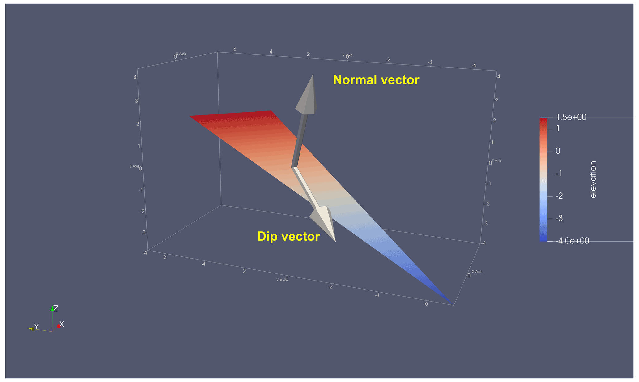
Figure 1A triangle with its normal and dip vectors. These two representations are used in our study for clustering.
3.1 Calculating the orientation
Three noncollinear points in three-dimensional space define a plane whose orientation can be calculated using basic linear algebra (Allmendinger, 2020; Groshong, 2006). When triangulation of the points is applied, the quality of the triangles can be measured using a variety of nonequivalent coefficients for their further removal (Collon et al., 2015; Michalak, 2018; Frey and Borouchaki, 1999). In this study, we used a collinearity coefficient defined as the proportion of the longest triangle edge to the length sum of the remaining edges (Michalak, 2018). The resulting coefficient lies within the interval of [0.5,1], with lower values pointing at equilateral triangles and higher values representing collinear configurations. In the irregular grid (which is the case for the Kraków–Silesian Homocline case studies), we filtered the configurations whose collinearity exceeded 0.90. This restriction resulted primarily in the removal of triangles that lie at the edge of the convex hull (see, e.g., the nonconvex shape of the convex hull in Fig. 12).
3.2 Assumptions underlying the clustering procedure
Selected clustering algorithms allow dissimilarity metrics to be specified to evaluate the similarity (or dissimilarity) between individual observations. In our case, these observations are normal and dip vectors (Fig. 1). For example, if the k-means algorithm is used (James et al., 2013), the squared Euclidean distance acts as the distance metric between p-dimensional observations xi and (in our case p=3):
We propose using the well-known fact (Choi et al., 2014; Zhang et al., 2020) that for unit normal vectors, the above squared distance is proportional to cosine distance (“∘” denotes the scalar product between two vectors, and || ⋅ || is the Euclidean norm):
Thus, the optimization problem solved in the k-means algorithm for unit vectors can be conceptualized in two ways (using the fact that the cos(x) takes values on the interval ).
- A.
Minimizing the within-cluster cosine distance: is minimized (equals zero) when , i.e., when the angle between xi and is 0∘.
- B.
Maximizing the between-cluster cosine distance: is maximized (equals two) when , i.e., when the angle between xi and is 180∘.
3.3 Equivalence of k-means clustering and Voronoi cells
Because the clusters resulting from applying the k-means algorithm can be conceptualized as Voronoi cells (Hastie et al., 2009), we propose explaining some of the clustering results using relevant computational geometry theorems about Voronoi diagrams (De Berg et al., 2008).
Let P be a set of n point sites in the plane. If all the sites are collinear then Vor(P) consists of n−1 parallel lines. Otherwise, Vor(P) is connected, and its edges are either segments or half lines.
For the Voronoi diagram Vor(P) of a set of points P the following holds:
- (i)
A point q is a vertex of Vor(P) if and only if its largest empty circle CP(q) contains three or more sites on its boundary.
- (ii)
The bisector between sites pi and pj defines an edge of Vor(P) if and only if there is a point q on the bisector such that CP(q) contains both pi and pj on its boundary but no other site.
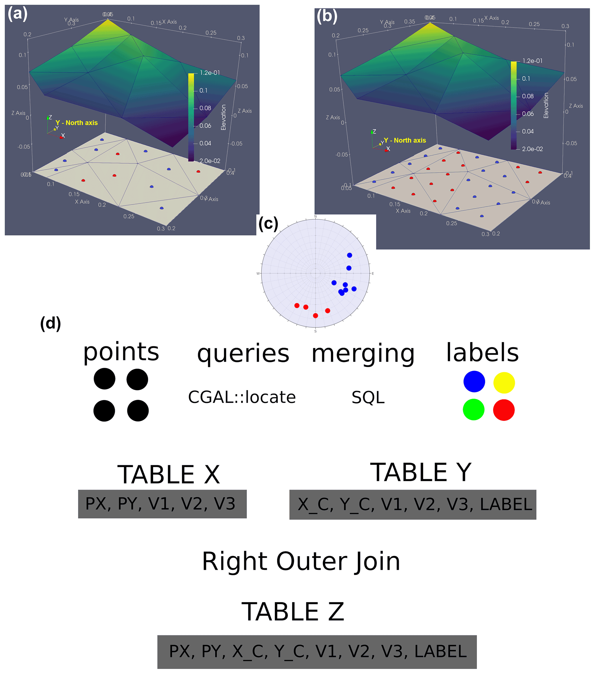
Figure 2Two versions of spatial clustering conducted on a geological contact: (a) geometric centers corresponding to Delaunay triangles selected, (b) regular grid based on CGAL queries and merging techniques, (c) orientation partitioning with respect to which the trends are visualized (we used lower hemisphere for dip vector representation), (d) a scheme presenting the role of CGAL (CGAL::locate) queries and merging (right outer join) techniques in obtaining the final result. A summary of the regularization method: information about clustering labels of triangles must be attached to points from the regular grid. This transfer of information is possible via CGAL query functions which allow triangles that have points in their interiors to be identified (the points are arguments of the query functions). Please note that execution of the query functions and clustering are done in separate environments; therefore two datasets (Table X and Y) need to be merged using unique elements (IDs of the vertices of triangles).
3.4 Irregular and regular trend maps
We propose here two versions of spatial clustering of geological contacts. The first version is based on taking one representative associated with the interiors of Delaunay triangles (their geometric centers). The vertices corresponding to the Delaunay triangles are given indices that are also included in the resulting data frame, which we denote as Table Y. The clustering methods assign the resulting orientation labels to the geometric centers of the Delaunay triangles (Fig. 2).
The second version tries to evenly represent the geometric trends throughout the deformed surface (Fig. 2). It allows the question to be answered as to whether a specific 2D point p (a geographic location) lying in the domain of a triangulation T is affected by a 3D geometric anomaly related to a triangulation model T. In this approach, a structured grid defined by points linked with corresponding clustering labels is generated. From a technical viewpoint, it is first necessary to generate the orientations of the Delaunay triangles. Then, we generate a regular point network within a region of interest. Next, we use the locate function offered by the Computational Geometry Algorithms Library (CGAL) to link the points from the regular network with the corresponding triangles. In its simplest version, this function takes the point query as its argument, and the possible return values are as follows (Yvinec, 2021):
-
If the point (from the regular network) query lies inside the convex hull of the points, a face that contains the query in its interior or on its boundary is returned.
-
If the point query lies outside the convex hull of the triangulation but in the affine hull, it is a face (∞, p, q) such that the query lies to the left of the oriented line (the rest of the triangulation lies to the right of this line).
In the code, we enable only the inclusion of the first group of triplets into the resulting data frame, which we denote here as Table X. To ultimately link the points from the regular grid (included in Table X) with the orientation labels (Table Y), the corresponding data frames need to be merged. Note that Table Y includes all available observations, but this is not the case for Table X. This is because not all triangles (e.g., those of small size) may be linked with any points from the user-defined regular grid, and this can especially be the case if the grid is sparse. To observe the differences, we therefore recommend using a SQL-related right outer join (ROJ) (or left outer join with replaced arguments) method rather than inner join for merging. The ROJ method returns all records from the right table and the matching records from the left table. This choice allows us to calculate the proportion of the area that is not covered with any orientation label (the coverage presented in Fig. 12). ROJ applied to Tables X and Y returns all rows from the right Table Y and any rows with matching keys from the left Table Y. In this study, the keys over which the tables are merged are the indices of the points that build the corresponding Delaunay triangles. If no points can be found for a given triangle, NA values are assigned to the px and py coordinates in the merged Table Z.
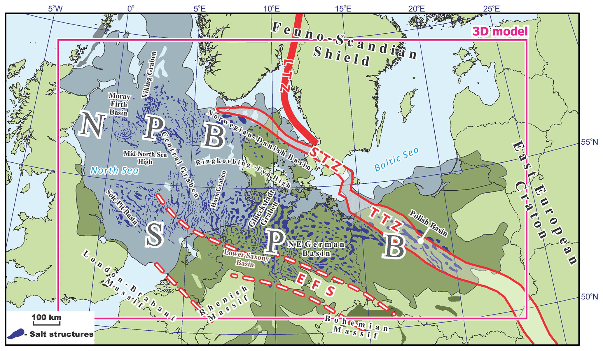
Figure 3Tectonic settings within the Central European Basin System with the location of the regional-scale 3D structural model (Maystrenko and Scheck-Wenderoth, 2013; Maystrenko et al., 2013, 2012). LTZ is according to (Medhus et al., 2012). Abbreviations: EFS – Elbe Fault System, LTZ – Lithospheric Transition Zone, NPB – Northern Permian Basin, SPB – Southern Permian Basin, STZ – Sorgenfrei–Tornquist Zone, and TTZ – Teisseyre–Tornquist Zone.
4.1 Case study 1: the Central European Basin System
The sedimentary cover of the Central European Basin System (CEBS) can be subdivided into three clearly distinguished structural levels: (1) pre-Permian, (2) Permian, and (3) Mesozoic–Cenozoic structural units (Doornenbal et al., 2009; Evans et al., 2003; Maystrenko et al., 2013, 2012; Ziegler, 1990b). The pre-Permian sedimentary level mainly includes Devonian and Carboniferous sedimentary rocks with Silurian, Ordovician, and Cambrian rocks along the northeastern margin of the CEBS (Doornenbal et al., 2009; Evans et al., 2003; Fossen et al., 2017; Lassen and Thybo, 2012; Usaityte, 2000; Wiest et al., 2020).
In the Late Carboniferous–Early Permian, the CEBS area was affected by the regional-scale rifting with deposition of mainly clastic sediments within the Northern and Southern Permian basins (Abramovitz and Thybo, 2000; Benek et al., 1996; Dadlez et al., 1995; Heeremans et al., 2004; Maystrenko et al., 2008; Plein, 1990; Stemmerik et al., 2000; Ziegler, 1990b). During the Middle–Late Permian time, a large amount of Zechstein rock salt, anhydrite, and carbonates accumulated within the Permian basins (Geluk, 2000; Maystrenko et al., 2008; Plein, 1990; Ziegler, 1990b). The Zechstein salt was reactivated during the Mesozoic and Cenozoic to form various salt structures within the CEBS (Fig. 3) (Doornenbal et al., 2009; Evans et al., 2003; Maystrenko et al., 2012, 2013).
Several pulses of active tectonics characterized the post-Permian evolution of the CEBS, including Triassic extension, Late Jurassic–Early Cretaceous extension and transtension, and Late Cretaceous–Early Cenozoic compression and inversion (Bell et al., 2014; Dadlez et al., 1995; Doornenbal et al., 2009; Erratt et al., 1999; Evans et al., 2003; Frederiksen et al., 2001; Graversen, 2002; Kyrkjebø et al., 2004; Mazur et al., 2016; Odinsen et al., 2000; Phillips et al., 2019; Scheck-Wenderoth and Lamarche, 2005; Vejbæk and Andersen, 2002; Ziegler, 1990b).
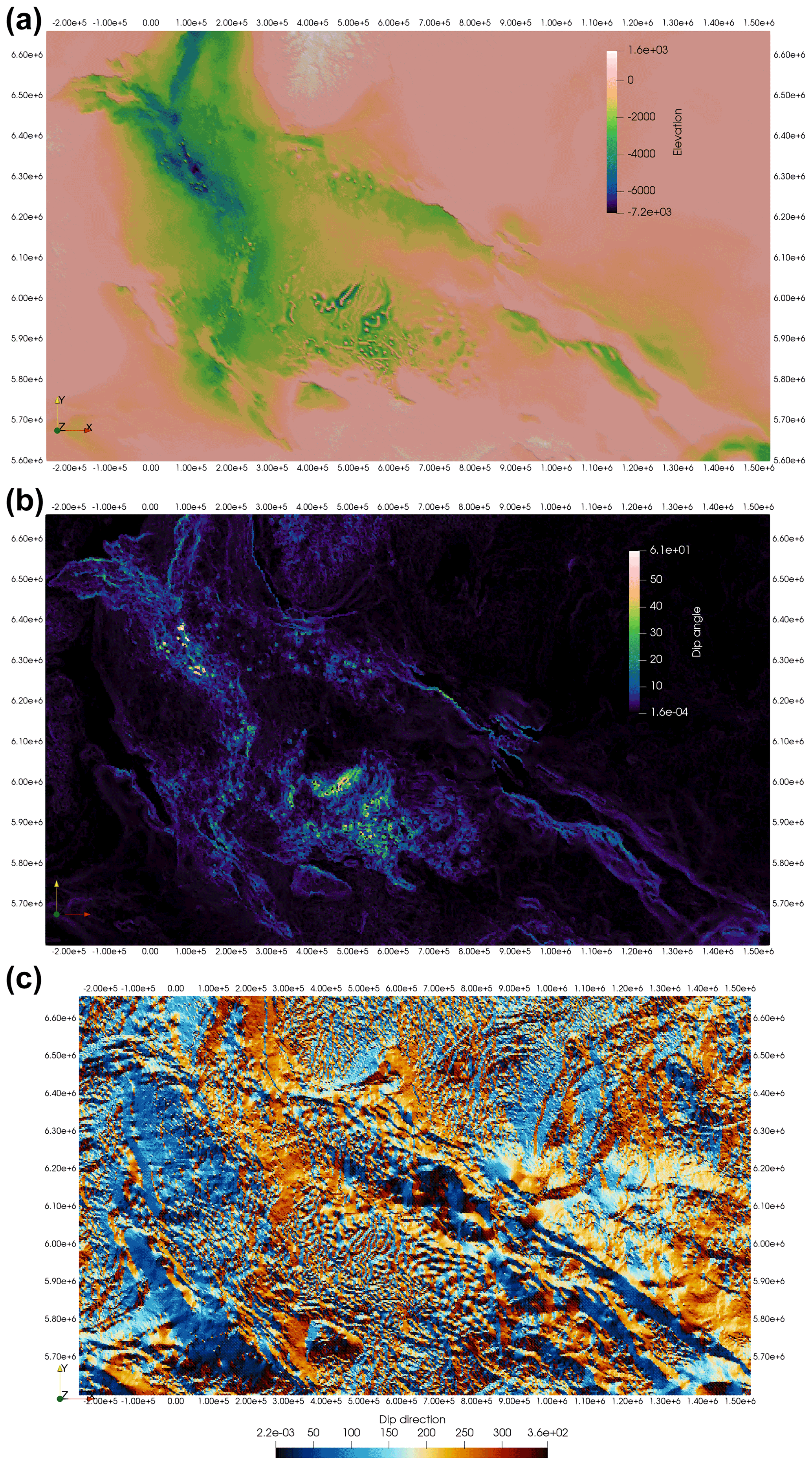
Figure 4(a) Hypsometry of the bottom Jurassic surface from the Central European Basin System. b Dip angle calculated for the bottom Jurassic surface. c Dip direction calculated for the Jurassic horizon. The boundaries between colors (a, b) are established without considering an optimization criterion.
The post-Permian tectonic events led to the formation of local sub-basins, superimposed on the Northern and Southern Permian basins (Figs. 3 and 4). The Norwegian–Danish Basin and the Central, the Viking, and the Horn grabens were formed within the Northern Permian Basin during the Triassic and the Jurassic–Early Cretaceous (Baldschuhn et al., 2001; Clausen and Korstgård, 1996; Erratt et al., 1999; Møller and Rasmussen, 2003; Phillips et al., 2019; Vejbæk, 1990). In the Southern Permian Basin, the Glueckstadt Graben together with the Northeast German and the Lower Saxony basins formed the broad North German Basin (Baldschuhn et al., 2001; Betz et al., 1987; Brink et al., 1990; Kockel, 2002; Maystrenko et al., 2005; Scheck et al., 2003), and the Polish Basin was superimposed on the eastern margin of the CEBS (Dadlez, 2003; Krzywiec, 2006). During the Late Cretaceous–Early Cenozoic, some parts of the CEBS underwent basin inversion, with the strongest compressive deformations and uplift along the Elbe Fault System and the Sorgenfrei–Tornquist and the Teisseyre–Tornquist zones (Hansen et al., 2000; Krzywiec et al., 2022; Mazur et al., 2005; Mogensen and Jensen, 1994; Otto, 2003; Scheck-Wenderoth and Lamarche, 2005; Voigt et al., 2008; Ziegler, 1990a). During the Cenozoic, broad subsidence occurred within the central part of the North Sea, where more than 3 km of sediments was deposited (Evans et al., 2003; Maystrenko et al., 2013; Ziegler, 1990b). The investigated Jurassic horizon represents the base of the Jurassic in places where the Jurassic sediments are present (Maystrenko et al., 2013, 2012). Within the rest of the model area, this horizon corresponds to the top of pre-Jurassic sediments or to the top of the crystalline basement.

Figure 5a Simplified geological map of Poland without Cenozoic formations (modified after Karnkowski, 2008; Osika et al., 1972) and the location of area studied. CZ – Częstochowa, FSH – Fore-Sudetic Homocline, HCS – Holy Cross Mountains, KSH – Kraków–Silesian Homocline, MS – Miechów Synclinorium, SM – Sudety Mountains. b Geological map of the studied part of the Kraków–Silesian Homocline (modified after Bardziński et al., 1986) and the location of the study area.
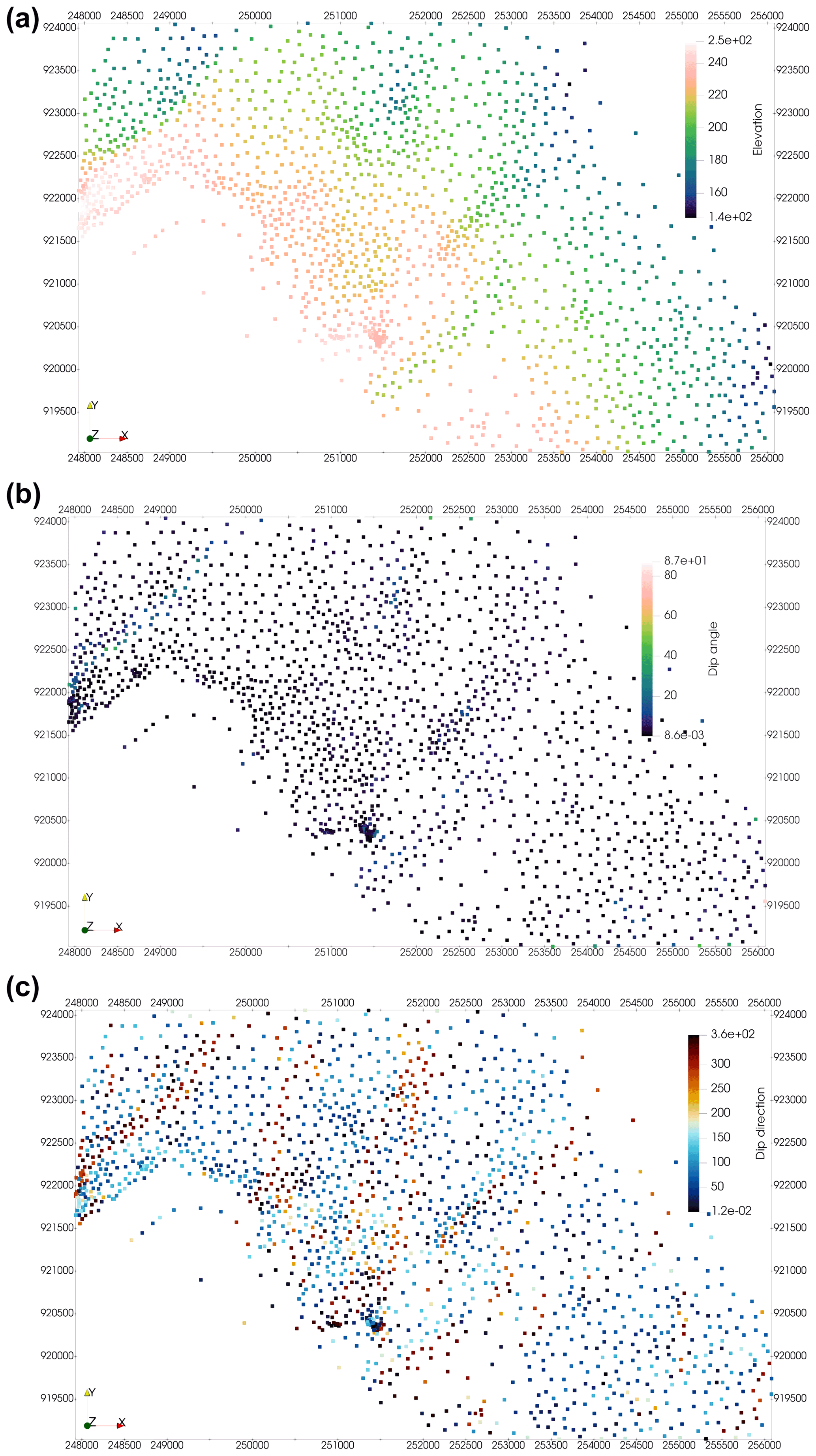
Figure 6a Hypsometry of the Jurassic horizon in Kraków–Silesian Homocline. b Dip angle calculated for the Jurassic horizon. c Dip direction calculated for the Jurassic horizon. The boundaries between colors are established without considering an optimization criterion, which results in the lack of spatial integrity of potential structures.
4.2 Case study 2: the Kraków–Silesian Homocline (KSH)
The KSH in Poland is interpreted as an eastern continuation of a greater geological unit called the Fore-Sudetic Homocline (Fig. 5) (Stupnicka and Stempień-Sałek, 2016; Mizerski, 2020; Narkiewicz, 2020). Both units are interpreted as natural slopes of the Szczecin–Łódź–Miechów Synclinorium formed during Late Cretaceous–Early Paleocene inversion of the Permian–Mesozoic Polish Basin (e.g., Dadlez et al., 1995; Słonka and Krzywiec, 2020). The axial part of the Permian–Mesozoic Polish Basin is called the Mid-Polish Trough and strikes parallel to the TTZ (see Mazur et al., 2021, for the latest interpretation of TTZ). The Mid-Polish Trough was a zone of strong subsidence during the Late Permian and Mesozoic (Kutek and Głazek, 1972). The inversion and uplift of the Polish Basin resulted in the formation of the Mid-Polish Anticlinorium, with two synclinoria symmetrically distributed along the NW–SE-trending anticlinorium (Fig. 5; Kutek and Głazek, 1972; Narkiewicz, 2020).
The Permo–Mesozoic deposits of the KSH represent predominantly clastic and carbonate series with common hiatuses and lie unconformably on the denuded and morphologically diversified Paleozoic or Precambrian basement (Buła et al., 2015). It is generally assumed that the strata along with accompanying geological contacts dip gently toward the northeast, a feature that has been present since the Late Cimmerian phase (Górecka, 1993; Krokowski, 1984). The layers were ultimately tilted to the northeast (Figs. 5 and 6), in the direction of the Szczecin–Łódź–Miechów Synclinorium axis, during the inversion of the Mid-Polish Trough in the Maastrichtian and Paleocene (Górecka, 1993; Kutek and Głazek, 1972). Deviations from the preferred direction of the dip to the northeast can be observed in the southeastern part of the KSH, where layers may dip to the south (Krokowski, 1984). The latter effect is believed to be caused by the thrusting Carpathians and the corresponding bending of deposits north of the thrusting loads in the Miocene (Jarosiński et al., 2009; Krokowski, 1984). Additionally, locally greater angular dip angles are expected to be found near faults due to fault-related bending of strata (Bednarek et al., 1992; Matyszkiewicz and Krajewski, 1996; Krokowski, 1984). It is important to note that some of the observed or hypothesized faults have received kinematic interpretations. For example, the én echelon arrangement of SW–NE-trending faults (Fig. 5) is believed to be formed by the underlying dextral movement of a strike-slip fault (Krokowski, 1984). This hypothesized movement, trending SE–NW, is believed to be related to the parallel Kraków–Lubliniec Fault, which separates blocks of crystalline basement (Buła et al., 2015).
For this study, we selected the geological interface that separates older Kościeliska sandstones (Early Bajocian–Late Bathonian) (Kopik, 1998) from the younger Częstochowa Ore-Bearing Clay Formation (Late Bajocian–Late Bathonian) in the area of the town of Nowa Wieś. The Częstochowa Ore-Bearing Clay Formation (known also as the ore-bearing clays) contains several horizons of siderite concretions, exploited in the past as the iron ore. There is a hiatus between the sediments, evidenced by the lack of a Strenoceras subfurcatum ammonite zone (Zakrzewski, 1976).
5.1 Case study 1 (CEBS) – materials
We used the lithosphere-scale 3D structural model of the CEBS, constructed by Maystrenko et al. (2013, 2012) and Maystrenko and Scheck-Wenderoth (2013), as the primary structural skeleton. The horizontal resolution of the model (grid spacing) is 4000 m. Vertically, the 3D model consists of 17 layers, 9 of which are the following sedimentary layers: Cenozoic, Cretaceous, Jurassic, Triassic, Permian salt, Permian carbonates, Rotliegend sediments, Permo-Carboniferous volcanics, and pre-Permian sedimentary rocks. In addition, the 3D structural model of the CEBS includes six layers of the crystalline crust and one layer for the lithospheric mantle. All depth interfaces, such as structural bases of sedimentary layers, top of the crystalline basement, Moho, and the lithosphere–asthenosphere boundary, can be extracted from the model. In this study, a base of the Jurassic has been taken to analyze the structural features of the CEBS (with exceptions mentioned at the end of Sect. 4.1). The lithosphere-scale 3D structural model covers the entire Northern and Southern Permian basins (Fig. 3). The adjacent London–Brabant, Rhenish, and Bohemian massifs in the south and the Fenno-Scandian Shield and the East European Craton in the northeast are also partially covered by the model. The constructed model of the CEBS is based on the available structural data, such as boreholes, seismic data, and maps. A detailed description of the input data is given in Maystrenko et al. (2012, 2013, 2020). Here, we only mention the largest datasets used during the model construction. The main data source for the 3D model was the North Sea Digital Atlas, which covers the entire North Sea (PGS, 2003). The digital version of the Geological Atlas of the Netherlands has been used for the Netherlands (NITG, 2004). To cover the North German Basin, the Geotectonic Atlas of northwestern Germany (Baldschuhn et al., 2001), the 3D structural model of the Glueckstadt Graben (Maystrenko et al., 2006), and the 3D model of the NE German Basin (Scheck et al., 2003) have been taken. The 3D crustal-scale model of the Polish Basin (Lamarche and Scheck-Wenderoth, 2005) has been used for Poland.
5.2 Case study 2 (KSH) – materials
We used 810 borehole records (Geological Company of Częstochowa, unpublished, the borehole dataset, 1950) that were handed over to the University of Silesia in Katowice by the “Geological Company of Częstochowa” (Częstochowskie Przedsiębiorstwo Geologiczne). The digitized version of these records contains Cartesian coordinates for the studied interface. The uncertainty in the borehole paths was not provided, and the precision of the coordinates was 1 cm. We used Pulkovo 1942(58)/Poland zone V (EPSG: 2175) as the coordinate reference system. Compared to a previous study built upon this dataset (Michalak et al., 2019), we filtered the data to minimize the number of “noisy” boreholes that are most likely related to measurement errors. The assumed errors were manifested as unusual pointwise-distributed depressions or elevations of the studied surface.
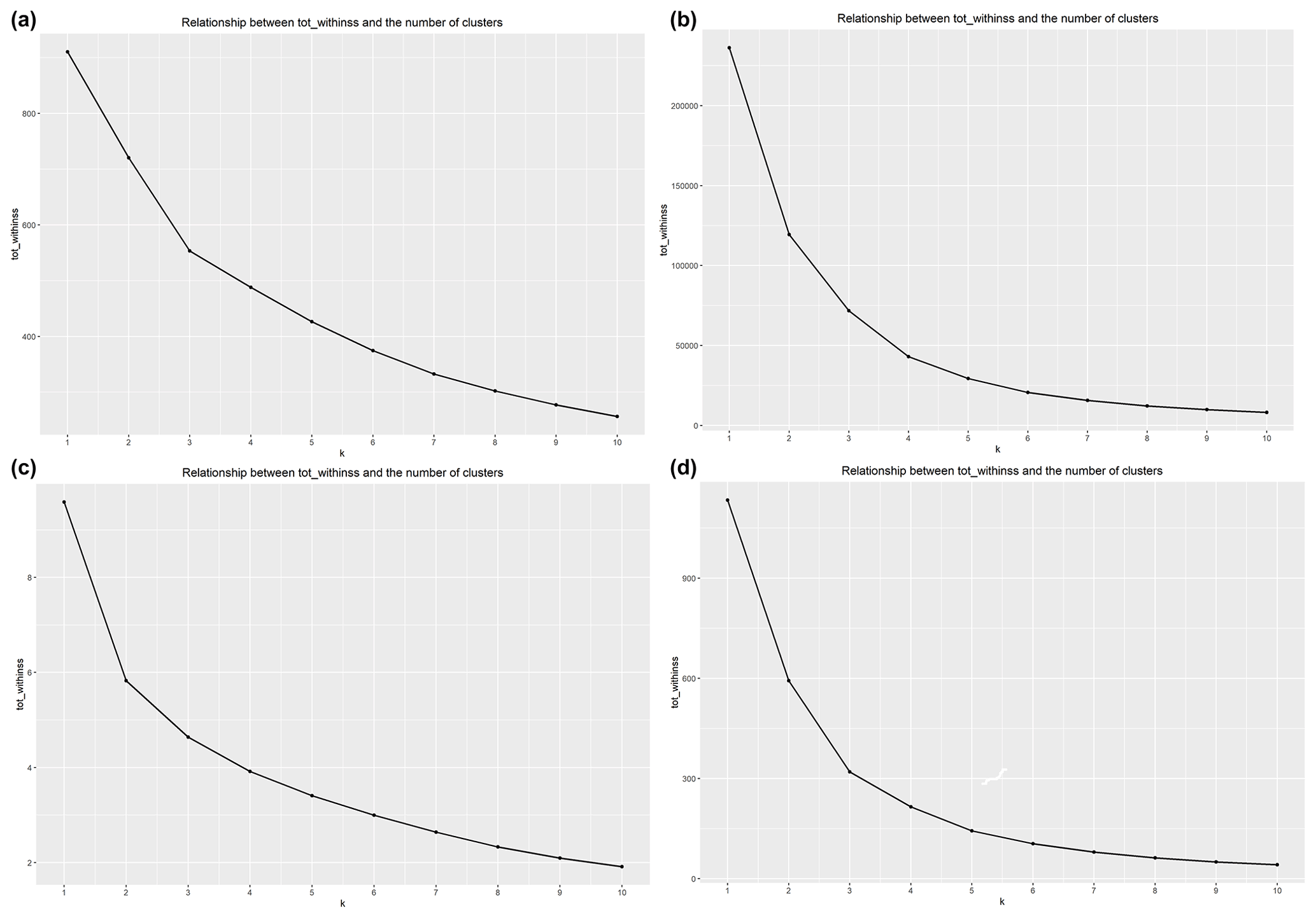
Figure 7The elbow method to determine the optimal number of clusters. It was applied to different case studies: (a) CEBS with normal vector representation, (b) CEBS with dip vector representation, (c) KSH with normal vector representation, (d) KSH with dip vector representation. Values on x axis denote the potential optimum number of clusters (), and tot_withinss on the y axis denotes the total within-cluster sum of squares: given a clustering partition, for every cluster the within-squares sum is calculated (), and finally tot.withinss = . In Hastie et al. (2009) tot_withinss is denoted as W(C), where C is a classification function. For example C(7) = 3 means that the third cluster was assigned to the seventh observation.
6.1 Determining the optimum number of clusters
An important clustering issue is the selection of the number of clusters. There are many competitive heuristics suggesting the optimal number of clusters (Rousseeuw, 1987; Hastie et al., 2009). Since in this study we only use the k-means algorithm, we followed the idea of the elbow method. It requires running the k-means algorithm for different k (e.g., from 1 to 10) and to compute the total within-squares sum for each clustering (denoted as tot_withinss in Fig. 7). To locate the optimal number of clusters, one looks for a kink in the sum-of-squares curve (Hastie et al., 2009). The experimental results usually suggest the optimum number of clusters to be two (Fig. 7b and c), three (Fig. 7a and d), or four (Fig. 7b).
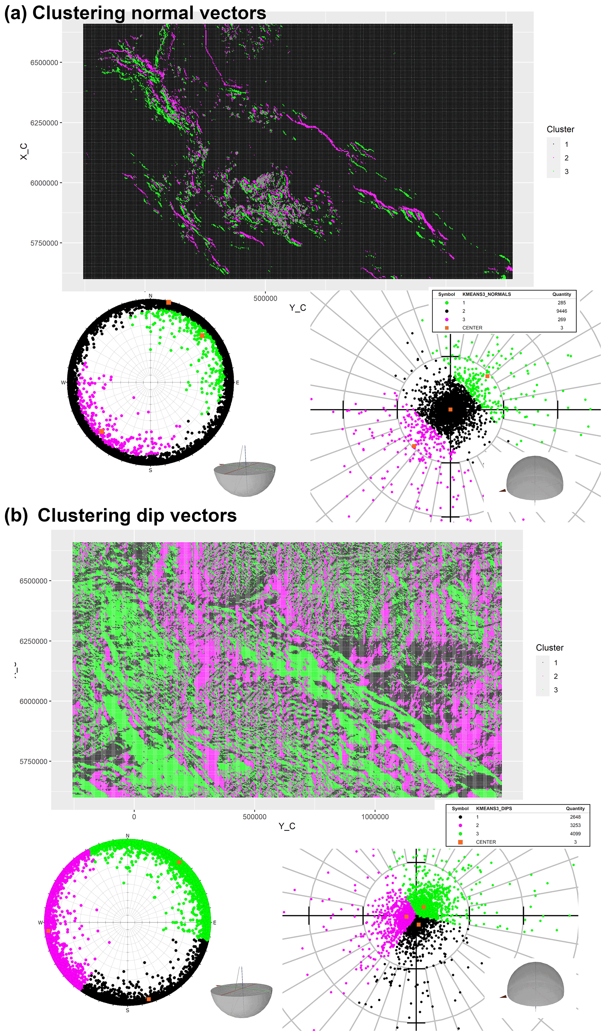
Figure 8Using k-means (k=3) clustering for normal (a) and dip (b) vectors for the investigated CEBS Jurassic horizon (irregular version). We used 236 380 observations for clustering, but the visualization is based on a random sample (10 000 observations). It can be observed that the normal representation (a) generated two sets of clusters, with the less represented (both less than 3 %) magenta and green clusters dipping at moderate angles to the southwest and northeast, respectively. Clustering dip vectors (b) resulted in partitions that represent three dip direction domains (NE, W, and SSE) with a common vertex near the stereonet origin and cluster centers having similar dip angles. Dip and dip direction of cluster centers are given in Table 1. The grid spacing is 10∘ for dip angles and dip directions. We applied a polar equal-angle stereographic projection. The left stereonet presents the projection of points from the unit lower hemisphere (tips of unit dip vectors) onto the horizontal plane. The stereonet on the right presents the projection of points from the unit upper hemisphere (tips of unit normal vectors) onto the horizontal plane.

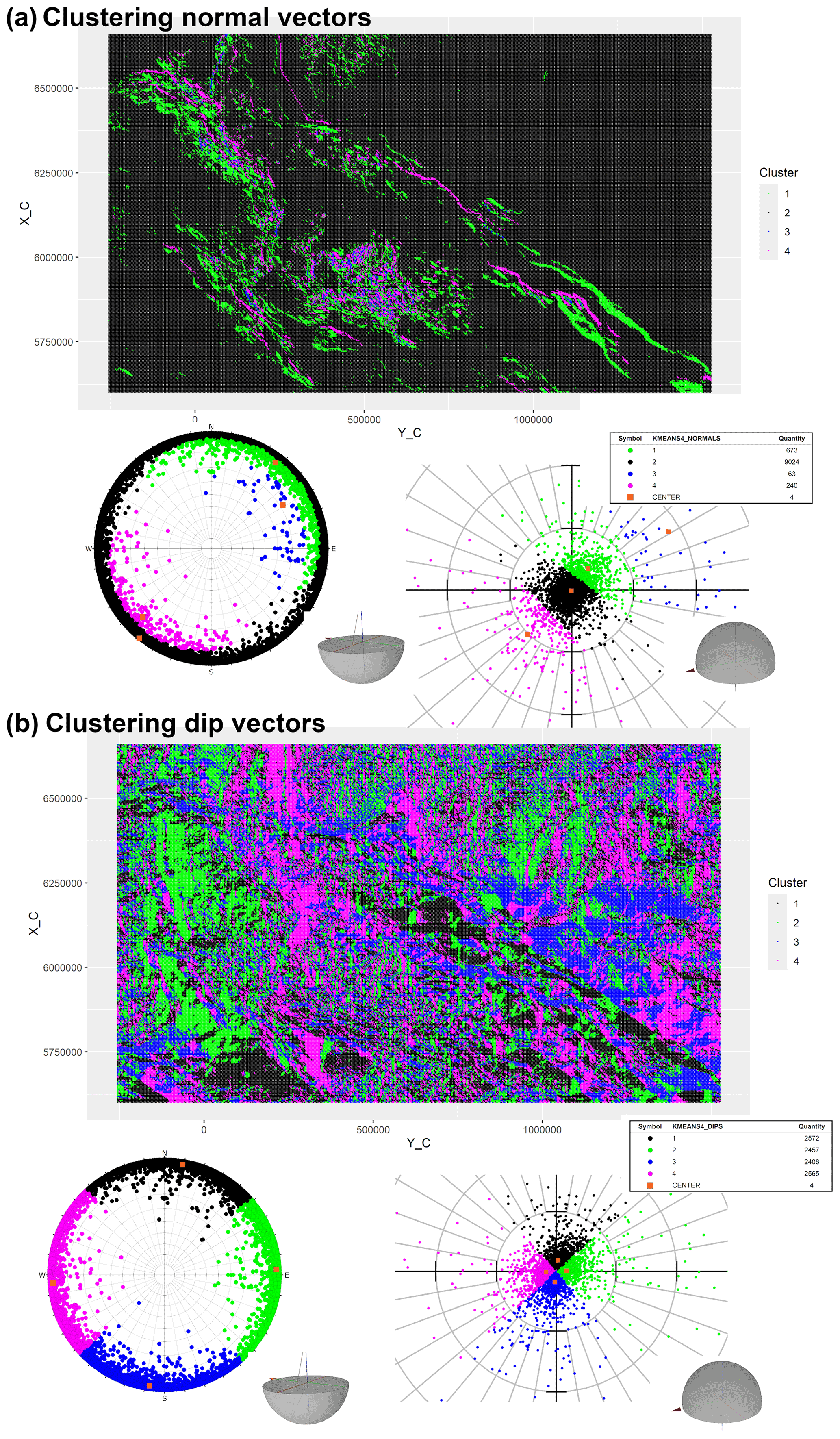
Figure 9Using k-means (k=4) clustering for normal (a) and dip (b) vectors for the investigated Jurassic horizon (irregular version). We used 236 380 observations for clustering, but the visualization is based on a random sample (10 000 observations). It can be observed that the normal representation (a) generated almost collinear cluster centers (NW–SE). Clustering dip vectors (b) resulted in partitions that represent four dip direction domains – NNE (black), W (magenta), E (green), and SSW (blue) – with a common vertex near the stereonet origin and cluster centers having similar dip angles. Dip and dip direction of cluster centers are given in Table 1. The grid spacing is 10∘ for dip angles and dip directions. For explanations regarding the projections, see the caption to Fig. 8.
6.2 Case study 1 (CEBS) – results
The linear, anomalous zones are obtained along the NW–SE-trending lithosphere-scale fault zones, such as the Tornquist Zone (the Sorgenfrei–Tornquist and the Teisseyre–Tornquist zones) in the northeast and the Elbe Fault System in the southwest (Figs. 4, 8, and 9). This is due to the fact that these fault zones controlled the structure of the crystalline basement and the configuration of the sedimentary cover within the CEBS that is reflected by the spatial clustering in Fig. 9a and b. In particular, the structural development of the Permo–Mesozoic Polish Basin is strongly coupled with the Teisseyre–Tornquist Zone, which can be considered to be the preexisting lithospheric weak zone beneath this basin (Mazur et al., 2021). The Teisseyre–Tornquist Zone is characterized by two wide zones of similar dip direction with low to moderate dip angle (Figs. 4c and 9b), reflecting the NW–SE strike of the Polish Basin (Fig. 5). In the case of the Sorgenfrei–Tornquist Zone, the northeastern margin of the Norwegian–Danish Basin was significantly affected by the shape of this fault zone during both the Permo–Mesozoic subsidence and the Late Cretaceous uplift (Erlström et al., 1997). A similar situation is along the Elbe Fault System, which is also represented by a zone of weakness at the southwestern margin of the North German Basin (Scheck et al., 2002). Another area with a set of the linear anomalous zones is located within the North Sea (Figs. 4 and 9b), where the Moray Firth Basin and the Central and Viking grabens are located (Fig. 3). There, these linear anomalous zones are mainly caused by the major boundary faults of the graben structures with the mentioned sedimentary basins. The sedimentary cover is faulted and folded along the boundary faults, and, therefore, the geometric anomalies follow the configuration of the faults.
The anomalous zones with smaller linear size and higher dip angles are most pronounced within the North German Basin, the Central Graben, the Horn Graben, and the eastern part of the Norwegian–Danish Basin, where the sedimentary cover is pierced and strongly deformed by large salt structures (Figs. 4 and 9a). The largest anomalies are obtained within the Glueckstad Graben and outline the NE–SW-trending, long and wide salt walls located there. Actually, the large size of the anomalies and high dip angles correlate well with the high intensity of salt movements, which were the strongest within the Glueckstad Graben (Maystrenko et al., 2013; Trusheim, 1960; Warsitzka et al., 2019). The high dip angle of the small-scale anomalies is obtained within the northern part of the Central Graben, where the salt diapirs pierce and strongly deform the sedimentary layers in the vicinity of salt structures (Davison et al., 2000; Karlo et al., 2014; Rank-Friend and Elders, 2004). The salt movements were also intensive within the Polish Basin (Krzywiec, 2004, 2012). However, the salt-induced deformations of the sedimentary cover of the Polish Basin are not clearly reflected by spatial clustering analysis compared to the Glueckstadt Graben or Central Graben. This is mostly related to a relatively low resolution of the data which have been used to construct the 3D structural model of Poland (Lamarche and Scheck-Wenderoth, 2005). In contrast, the input data for the Glueckstadt and Central grabens were characterized by higher resolution (Baldschuhn et al., 2001; PGS, 2003), allowing the authors to include more details of the basin structures in the grabens.
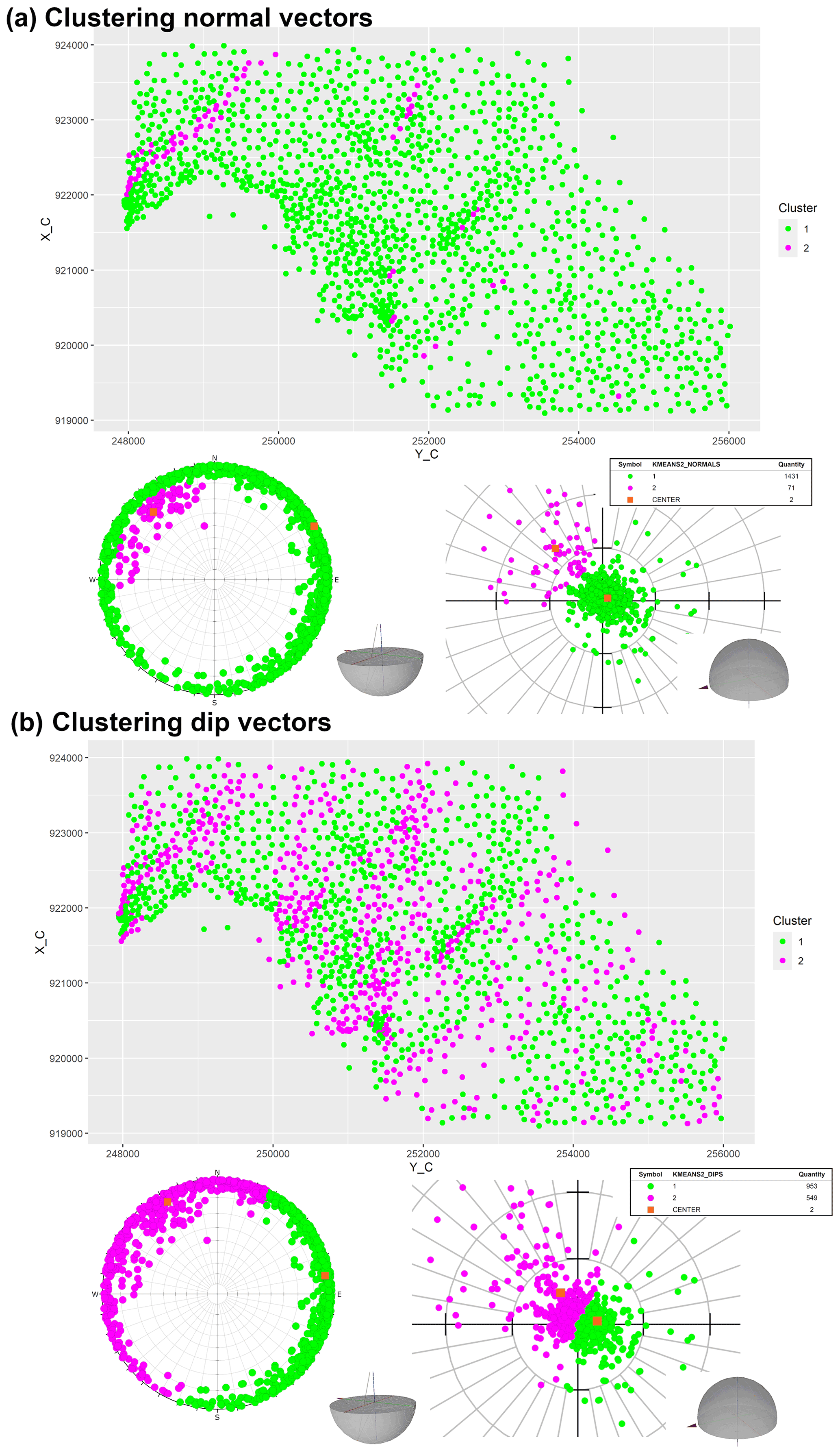
Figure 10Using k-means (k=2) clustering for normal (a) and dip (b) vectors for the investigated KSH Jurassic horizon. This version is irregular: orientation labels are assigned to geometric centers of Delaunay triangles. Both clustering and visualizations are based on 1502 observations. It can be observed that the normal representation (a) generated two sets of clusters, with the less represented (about 4.7 %) magenta cluster dipping at moderate angles to the northwest. Clustering dip vectors (b) resulted in partitions that represent two dip direction domains, with NW and ENE centers having similar dip angles. Dip and dip direction of cluster centers are given in Table 2. The grid spacing is 10∘ for dip angles and dip directions. For explanations regarding the projections, see the caption to Fig. 8.
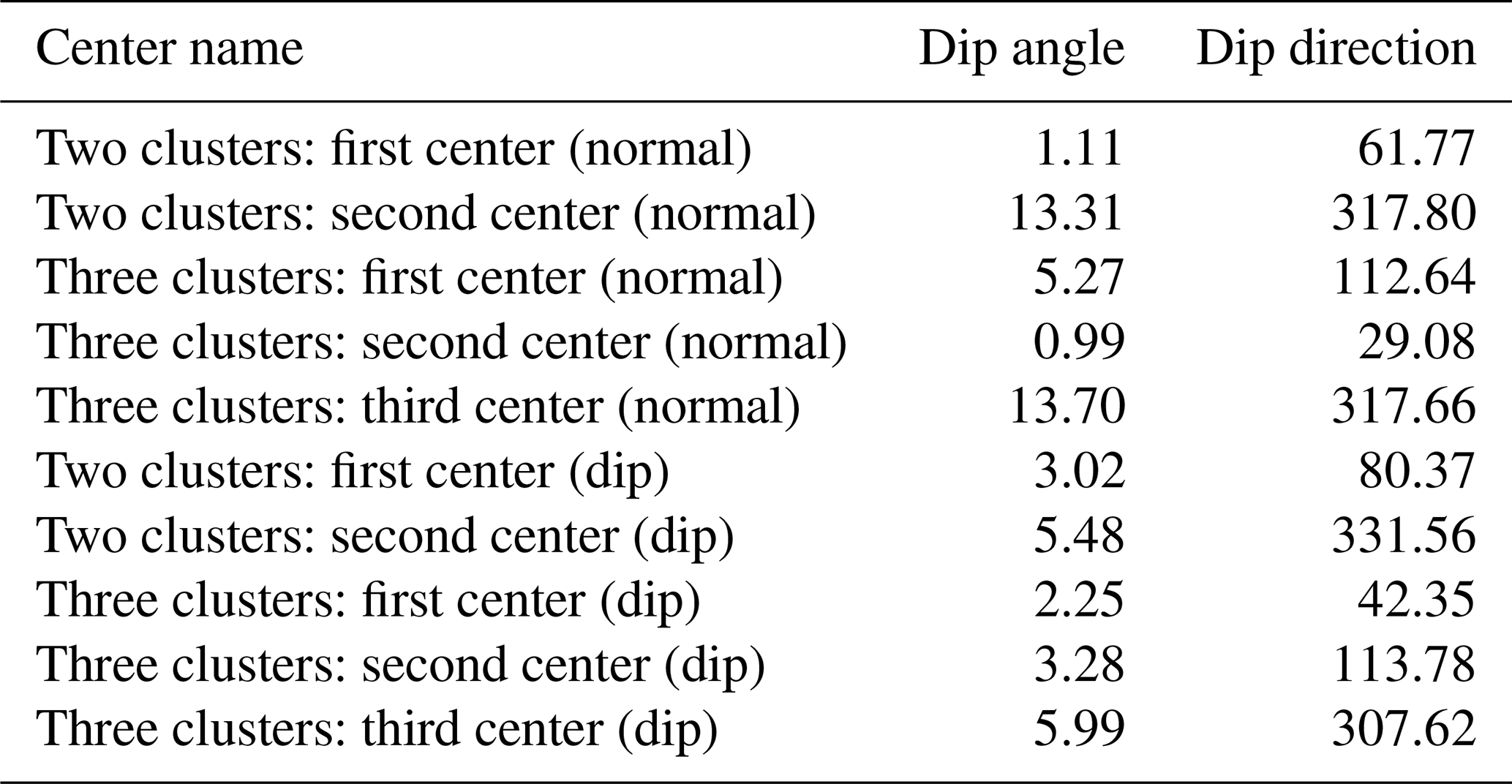
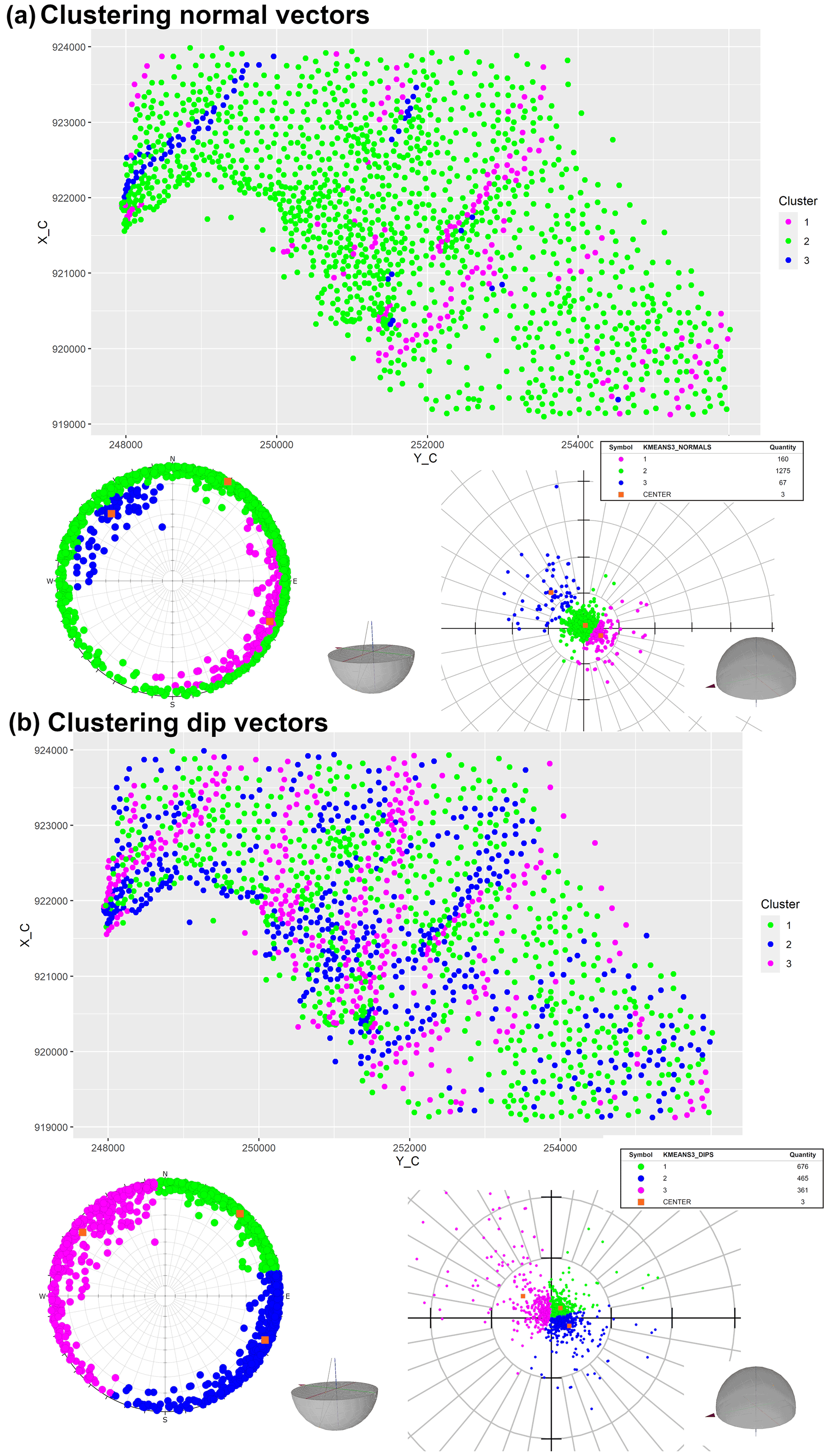
Figure 11Using k-means (k=3) clustering for normal (a) and dip (b) vectors for the investigated KSH Jurassic horizon. This version is irregular: orientation labels are assigned to geometric centers of Delaunay triangles. Both clustering and visualizations are based on 1502 observations. It can be observed that the normal representation (a) generated three sets of clusters, with the less represented (about 10.7 %) magenta and blue (about 4.5 %) clusters dipping to the northwest and southeast, respectively. The boundaries between clusters have a similar NE–SW trend. Clustering dip vectors (b) resulted in partitions that represent three dip direction domains, with NW, NE, and ESE centers having similar dip angles. Dip and dip direction of cluster centers are given in Table 2. The grid spacing is 10∘ for dip angles and dip directions. For explanations regarding the projections, see the caption to Fig. 8.
6.3 Case study 2 (KSH) – results
Both the normal (Figs. 10a and 11a) and dip vector representations (Figs. 10b and 11b) reveal similar spatial configurations of geometric anomalies, i.e., observations dissimilar to the subhorizontal dip to the northeast. A visible difference between normal and dip vector representation can be attributed to the spatial integrity of W–E-trending anomalies (dipping to the south), which is not very well preserved in the normal vector representation with three clusters. This effect can be explained by the fact that in the normal representation with three clusters, the cluster centers are more or less collinear. This suggests (Theorem 1) that in the normal vector representation, boundaries between clusters are more or less parallel. Indeed, in our results the boundaries between clusters seem to have a similar NE–SW trend (Fig. 11a). The implication of this result is that observations dipping to the south may be assigned to more than one cluster (magenta and green) when normal vectors are used for clustering.
For the two representations, two distinctly trending sets can be observed: NE–SW and NNE–SSW (locally N–S). The presence of an én echelon arrangement of the NE–SW set is in line with the orientation of faults in the Częstochowa region (Fig. 5b; Bardziński et al., 1986) and with the model of extensional faulting in the northern part of the KSH due to SE–NW-oriented dextral strike-slip movement (Krokowski, 1984). However, our results do not support the unimodal distribution of fault strikes (only NE–SW), as proposed by (Bardziński et al., 1986; Fig. 5b).
We see that some of the arrangements are composed of more than one observation in the direction perpendicular to their trend (e.g., the SW–NE-trending anomaly in the NW part of the area in Fig. 10b). This necessitates discussion about the origin of these forms given that the difference in elevation between a hanging wall and footwall can be consumed by a single triangle (e.g., with two points lying on the hanging wall and the third on the footwall) (Michalak et al., 2021).
The above effect could be explained by several competitive hypotheses. For example, the fault plane could have been drilled, thus broadening the zone of triangles genetically related to the fault (Michalak et al., 2021). Assuming the tectonic origin of the related structures, it can be hypothesized that fault drags on the hanging wall contribute to subsidiary elevation differences that must be consumed by nearby triangles. It could also be argued that an unusual lowering of the contact surface is due to a deformation zone composed of many smaller faults. Another hypothesis could be that the related feature is not a fault but rather a sedimentary slope, which would explain the gradual lowering of the contact surface.
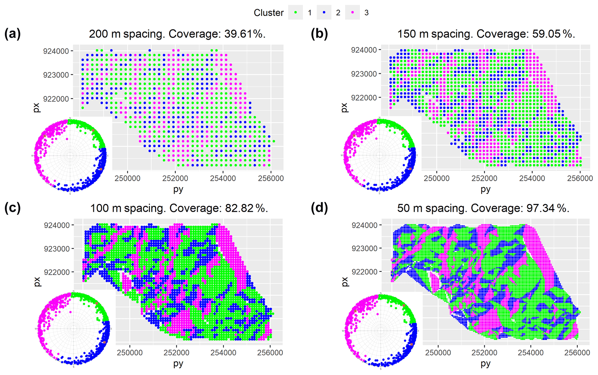
Figure 12Regular version of spatial clustering. Impact of the grid density on the geometric granularity of the studied interface: (a) grid with points separated by 200 m, (b) grid with points separated by 150 m, (c) grid with points separated by 100 m, and (d) grid with points separated by 50 m. The coverage rates refer to the proportion of filtered (not including collinear) Delaunay triangles linked with the points from the regular grid to all filtered Delaunay triangles. Note that exceptions from the convex shape of the polygon or blank spaces in the interior are due to removed collinear configurations. We recommend minimizing the value of spacing to exhibit potential connectivity patterns. The grid spacing is 10∘ for dip angles and dip directions. We applied a polar equal-angle stereographic projection. The stereonet presents the projection of points from the unit lower hemisphere (tips of unit dip vectors) onto the horizontal plane.
From a topological (Thiele et al., 2016) perspective, some of the NE–SW-trending arrangements are paired in that their NW- and SE-dipping counterparts are adjacent (e.g., the form composed of blue and magenta SW–NE-trending belts in the southern part of the area in Fig. 12c and d). Depending on their relative position, they can be interpreted either as paleovalleys, grabens, and synclines (negative forms) or peaks, horsts, and anticlines (positive forms). They can also be interpreted in terms of antithetic shear with hanging walls dipping against the main fault, which is often the case for listric faults (Harding and Tuminas, 1989; Fossen, 2006) or reverse drag or rollover anticlines (Fossen, 2006).
We also produced results using the regular version of spatial clustering with different coverage rates (Fig. 12a–d), i.e., proportions of triangles linked with points comprising the regular grid. These results show that lower coverage may result in the omission of small triangles (Fig. 12a and b), which can be misleading for analysis of connectivity between different representatives of the observed anomalies (Fig. 12c and d). The regular version allows the orientation of neighbors of triangles to be better observed, which can be more difficult if the irregular version is applied.
7.1 Method's capabilities
The method's promise to identify geometric anomalies lies in the fact that squared Euclidean distance inherent to the k-means algorithm (Hastie et al., 2009) is equivalent to cosine distance if processed vectors have unit length (Eq. 2). Thus, the resulting clusters have geometric meaning because they represent groups of observations that have small within-cosine distance, a fact often used in the field of text analysis (Choi et al., 2014; Zhang et al., 2020; Hornik et al., 2012). In structural studies, cosine distance as a dissimilarity metric was used for detecting fracture sets in outcrops (Zhan et al., 2017a) based on observations with substantial dip. In this study, we analyzed subsurface geological terrains with subhorizontal or moderate dip, and we believe that the method holds promise for providing insights into the subsurface architecture of similar class-imbalanced data, thus preventing the creation of oversimplified models (Caumon et al., 2009).

Figure 13An observed clustering pattern: (a) when normal vectors are clustered, the cluster centers are almost collinear. Theorem 1 says that collinear cluster centers imply parallel boundaries between clusters; this result suggests that the boundaries between clusters may point to an axis of a potential megacylinder. (b) When dip vectors are clustered, there is a common vertex for all clusters near the origin. This effect suggests (Theorem 2) that the centers are co-circular, which implies a common value of dip angle (compare dip angles for dip representations in Tables 1 and 2), thus pointing to a potential megacone. To improve the visibility of boundaries between clusters, we applied the stereonet, which presents the projection of points from the upper hemisphere (tips of unit normal vectors obtained from dip vectors) onto the horizontal plane. (c) A cylinder as a model for the partitioning results of normal vector representation. (d) A cone as a model for the partitioning results of dip vector representation.
This study adds knowledge regarding the possibility of using computational geometry theorems to explain the meaning of resulting clusters. As a case in point, we note that clustering results have a repeatable pattern in that the normal representation produced almost collinear cluster centers (Fig. 13a), and the dip representation always has (except k=2, when there is no vertex, and the theorem is not applicable) a vertex common for all clusters near the origin of the stereonet (Fig. 13b). These results can be rewritten using the computational geometry theorems. From Theorem 1 it follows that collinear cluster centers imply parallel boundaries between clusters. Indeed, in our results, the approximate boundaries between clusters have a similar trend (Fig. 13a). This suggests that in our results, the boundaries between clusters may be distributed along a potential cylinder axis with cluster centers lying in the same plane, which is perpendicular to the direction of a potential cylinder axis. Moreover, from Theorem 2 it follows that a point q is a vertex in Voronoi diagrams if and only if its largest empty circle CP(q) contains three or more sites on its boundary. Thus, in Fig. 13b, the cluster centers must have a very similar distance to the origin, which implies that the cluster centers lie approximately on a common circle and thus have a very similar dip angle (compare dip angles for dip representations in Tables 1 and 2). A full explanation of the above effects lies beyond the scope of this research and needs further studies.
7.2 Regularization
The first version is irregular, which means that we assign an orientation label to the geometric center of a triangle. This arbitrary decision makes the resulting map biased. The second version reduces the arbitrariness by creating a regular point set that is linked with corresponding triangles and their orientation labels. This regularization may serve to solve topological problems, e.g., whether or not the hypothesized faults intersect. However, there are two caveats to the regularization step:
-
Only the irregular version can provide additional insights into the observed features (e.g., explanatory hypotheses about drilling the fault plane or having a listric fault).
-
The regular version is still sensitive to the initial spatial heterogeneity of the data density (the spatial configuration of the boreholes).
If the analysis of connectivity between anomalies is of interest, our recommendation is to minimize the spacing of the points in the grid so as to maximize the proportion of linked triangles. This should be helpful to better analyze connectivity between observed anomalies. However, a sparse grid could be potentially more useful in the generalization schemes related to upscaling frameworks (Carmichael and Ailleres, 2016).
7.3 Limitations
Assuming the spatial homogeneity of the subhorizontal dip to the northeast (ideally a flat plane dipping to the northeast), the distances between three points taken to construct the plane do not influence its orientation (it is the same plane). However, if this homogenous surface is faulted, then triangles genetically related to the faults have orientations different to that of the underlying faulted surface (Michalak et al., 2021). The directional dissimilarity of the triangles genetically related to faults (thus anomalies) may sometimes be high, with nonintuitive dip directions of triangles opposite the fault dip direction (Michalak et al., 2021). In addition, the dip angle of these triangles is affected by the density of the borehole network in the vicinity of the fault, with boreholes located closer to the fault, resulting in relatively greater dip angles. This interplay between the initial technical conditions (dip angle of triangles genetically related to faults depends on density of boreholes) and tectonics may limit the epistemological value of the resulting interpretation based on dip-angle-informed clustering (e.g., Fig. 11A). We note that dip vectors are not uniquely defined for horizontal observations (the dip direction cannot be specified), so we recommend removing horizontal observations prior to conducting clustering. A similar problem and proposed solution applies to normal vectors of vertical observations, for which two possible dip directions can be given.
7.4 Expert-guided partitions
If the faults strike perpendicular to the preferred direction, then setting a threshold to dip angle may be helpful to reduce the interpretational impact of the initial technical conditions (the density of the borehole network). For example, if faults strike perpendicular to the preferred fault direction (NE) and have their hanging wall to the northeast, then the related triangles have dip angle values greater than that of the regional trend, irrespective of the spatial heterogeneity of boreholes. Therefore, we suggest that sometimes the assistance of expert knowledge is needed to answer more specific questions. Another argument in support of the expert-guided partition is that although the combination of dip vector representation and the squared Euclidean distance metric can help identify the directional domains, in some cases, the underlying assumption may not be realistic because genetically related observations may dip to opposite directions. Merging the two groups of observations with a dip direction difference of 180∘ is, however, unlikely if the combination of dip vector representation and the squared Euclidean distance (cosine distance for unit vectors) is applied (Figs. 10b and 11b). As a case in point, consider a fault striking perpendicular to the preferred dip direction (NE) with the hanging wall lying to the southwest. In this case, triangles genetically related to such a fault may dip to the southwest when the points from the hanging wall and footwall are relatively close to each other (and/or with a high value of fault throw). However, they may also dip to the northeast at smaller angles, which may be the case if the distance between the points from the hanging wall and footwall is relatively high (and/or with a small value of fault throw), thus only flattening the general effect of the dip to the northeast.
We note that the space of the geometric hypotheses created by the cartographic results may be high and thus interpretationally challenging. We note that in the case of a lack of other geological knowledge or data, the method is capable only of indicating the strike of the hypothesized structures. This is because the dip direction associated with the triangles related to these faults may also be attributed to reverse faults that have dip directions opposite those of the related triangles (Michalak et al., 2021).
As Bond (2015) argues, for much structural geology, it is fair to say that “it's all about geometry”. The infinite three-dimensional space encountered in structural geology observations points to the need for generalization of geometric information to increase the capabilities of recognizing related structures and their topology (Kania and Szczęch, 2020; Thiele et al., 2016). We believe that the workflow holds promise for identifying the relationships between the effects of the forces that shaped the region and those that caused subareas to deviate from the regional plan (compare Davis, 2002). More detailed conclusions are highlighted below.
Compared to simply color-coding surfaces with respect to either dip angle or dip direction, our method allows investigation of the relationship between dip and dip direction anomalies. Moreover, in simple visualizations of dip angle and dip direction, the boundaries between colors in available default color palettes are established without considering an optimization criterion, which may result in the lack of spatial integrity of the existing structures (Fig. 6c).
In our approach, observations are separated according to an optimization criterion. Our method is capable of detecting geometric anomalies because applying squared Euclidean distance to unit vectors results in minimizing within-cluster cosine distance (Eq. 2). Obviously, the geometric meaning of the proposed optimization procedure can be completely lost if the processed vectors do not have unit length. Thus, we do not recommend scaling vectors according to the size of the related triangles.
In the case of many subhorizontal observations (which is true for many terrains), we propose two different conceptualization about the optimization procedure for normal and dip representations. For normal vectors representing subhorizontal terrains, it is better to conceptualize the optimization as minimizing the within-cluster cosine distance. For dip vectors representing subhorizontal terrains, it is better to conceptualize the optimization task as maximizing the between-cluster cosine distance.
The correspondence between Voronoi tessellation (Hastie et al., 2009) and clusters resulting from applying the k-means algorithm as well as computational geometry theorems allows the meaning of the clusters to be further explained. Empirical results show that the combination of cosine distance with normal and dip vector representation holds promise for identifying axes of potential megacylinders and slope of potential megacones, respectively (Fig. 13). These results should not however be extrapolated as a general rule for other study areas.
The selection of triangulation as a source of collecting data for spatial clustering allows the internal structure of anomalies to be revealed. We created additional yet potentially competitive hypotheses about the nature of the observed anomalies, i.e., whether the internal structure of the singularity may be due to drilling a nonvertical fault plane or due to a wider deformation zone composed of many smaller faults.
Software for this research is available in the in-text data citation references (Michalak, 2021b): name of code – GeoAnomalia; license – GNU General Public License v3.0; developer – Michał Michalak; contact address – Institute of Earth Sciences, University of Silesia in Katowice, Poland; e-mail – michalmichalak@us.edu.pl; year first available – 2021; hardware required – Celeron CPU or better; software required – Microsoft Visual Studio (2015, 2017, 2022); program language – C; program size – 600 KB; how to access the source code – available at https://github.com/michalmichalak997/SurfaceCompare/blob/master/orientation_maps.cpp; setup guide – https://github.com/michalmichalak997/Triangulation_2/blob/master/README.md (last access: 27 October 2022).
Datasets for this research (input and processed data) are available on request at https://doi.org/10.5281/zenodo.6405496 (Michalak, 2021a).
MPM devised the project, wrote the manuscript, performed the computations, and discussed the results. LT discussed the results and created several hypotheses regarding the internal structure of the revealed anomalies. FW participated in the study conceptualization (formulating the idea of regularization) and discussed the results (creating hypotheses regarding the observed anomalies). JŻ drafted the regional geological setting and discussed the results regarding the internal structure of the observed anomalies. KG participated in drafting the regional geological setting. MK advocated for the regularization and discussed the limitations regarding the interpretational value of dip-angle-based clustering. YPM described the setting and data from the Central European Basin System and discussed the results. PL participated in drafting the regional geological setting.
The contact author has declared that none of the authors has any competing interests.
Publisher's note: Copernicus Publications remains neutral with regard to jurisdictional claims in published maps and institutional affiliations.
This study was financially supported by the National Science Centre, Poland (2020/37/N/ST10/02504). The license of the Dips 8.0 software was purchased by the AGH University of Science and Technology, grant number 16.16.140.315. Michał P. Michalak thanks Janusz Morawiec for discussions about cones as models for clustering results and Filip Turoboś for general discussions. We thank the reviewers Guillaume Duclaux and Thomas Blenkinsop for their constructive suggestions and critical questions, which helped better explain differences between the clustering results.
This research has been supported by the National Science Centre, Poland (grant no. 2020/37/N/ST10/02504), and the AGH University of Science and Technology (grant no. 16.16.140.315).
This paper was edited by David Healy and reviewed by Guillaume Duclaux and Thomas Blenkinsop.
Abramovitz, T. and Thybo, H.: Seismic images of Caledonian, lithosphere-scale collision structures in the southeastern North Sea along Mona Lisa Profile 2, Tectonophysics, 317, 27–54, https://doi.org/10.1016/S0040-1951(99)00266-8, 2000.
Allmendinger, R. W.: GMDE: Extracting quantitative information from geologic maps, Geosphere, 16, 1495–1507, https://doi.org/10.1130/GES02253.1, 2020.
Baldschuhn, R., Binot, S., Fleig, S., and Kockel, F.: Geotektonischer Atlas von Nordwest-Deutschland und dem deutschen Nordsee-Sektor — Strukturen, Struckurenwicklung, Paläogeographie, Geol. Jahrb., A153, 1–88, 2001.
Bardziński, W., Lewandowski, J., Więckowski, R., and Zieliński, T.: Objaśnienia do Szczegółowej Mapy Geologicznej Polski w skali 1:50 000, ark. Częstochowa (845), Wydawnictwa Geologiczne, Warszawa, 72 pp., 1986.
Bednarek, J., Haisig, J., Lewandowski, J., and Wilanowski, S.: Objaśnienia do Szczegółowej Mapy Geologicznej Polski 1:50 000, Arkusz Kłobuck (808), PIG, Warszawa, 66 pp., 1992.
Bell, R. E., Jackson, C. A. L., Elliott, G. M., Gawthorpe, R. L., Sharp, I. R., and Michelsen, L.: Insights into the development of major rift-related unconformities from geologically constrained subsidence modelling: Halten Terrace, offshore mid Norway, Basin Res., 26, 203–224, https://doi.org/10.1111/bre.12049, 2014.
Benek, R., Kramer, W., McCann, T., Scheck, M., Negendank, J. F. W., Korich, D., Huebscher, H. D., and Bayer, U.: Permo–Carboniferous magmatism of the Northeast German Basin, Tectonophysics, 266, 379–404, https://doi.org/10.1016/S0040-1951(96)00199-0, 1996.
Bergen, K. J., Johnson, P. A., De Hoop, M. V., and Beroza, G. C.: Machine learning for data-driven discovery in solid Earth geoscience, Science, 363, eaau0323, https://doi.org/10.1126/science.aau0323, 2019.
Betz, D., Führer, F., Greiner, G., and Plein, E.: Evolution of the Lower Saxony Basin, Tectonophysics, 137, 127–170, https://doi.org/10.1016/0040-1951(87)90319-2, 1987.
Bond, C. E.: Uncertainty in structural interpretation: Lessons to be learnt, J. Struct. Geol., 74, 185–200, https://doi.org/10.1016/j.jsg.2015.03.003, 2015.
Brink, H., Franke, D., Hoffmann, N., Horst, W., and Oncken, O.: Structure and evolution of the North German Basin, in: The European Geotraverse: Integrative Studies, edited by: Freeman, R., Giese, P., and Mueler, S., European Science Foundation, Strasbourg, 195–212 pp., 1990.
Buła, Z., Habryn, R., Jachowicz-Zdanowska, M., and Żaba, J.: The precambrian and lower paleozoic of the brunovistulicum (eastern part of the upper silesian block, southern Poland) – The state of the art, Geol. Q., 59, 123–134, https://doi.org/10.7306/gq.1203, 2015.
Carmichael, T. and Ailleres, L.: Method and analysis for the upscaling of structural data, J. Struct. Geol., 83, 121–133, https://doi.org/10.1016/j.jsg.2015.09.002, 2016.
Caumon, G., Collon-Drouaillet, P., Le Carlier De Veslud, C., Viseur, S., and Sausse, J.: Surface-based 3D modeling of geological structures, Math. Geosci., 41, 927–945, https://doi.org/10.1007/s11004-009-9244-2, 2009.
Cawood, A. J., Bond, C. E., Howell, J. A., Butler, R. W. H., and Totake, Y.: LiDAR, UAV or compass-clinometer? Accuracy, coverage and the effects on structural models, J. Struct. Geol., 98, 67–82, https://doi.org/10.1016/j.jsg.2017.04.004, 2017.
Choi, J., Cho, H., Kwac, J., and Davis, L. S.: Toward sparse coding on cosine distance, in: 2014 22nd International Conference on Pattern Recognition, 24–28 August 2014, Stockholm, Sweden, https://doi.org/10.1109/ICPR.2014.757, 2014.
Clausen, O. R. and Korstgård, J. A.: Planar detaching faults in the southern Horn Graben, Danish North Sea, Mar. Petrol. Geol., 13, 537–548, https://doi.org/10.1016/0264-8172(96)00001-3, 1996.
Collon, P., Steckiewicz-Laurent, W., Pellerin, J., Laurent, G., Caumon, G., Reichart, G., and Vaute, L.: 3D geomodelling combining implicit surfaces and Voronoi-based remeshing: A case study in the Lorraine Coal Basin (France), Comput. Geosci., 77, 29–43, https://doi.org/10.1016/j.cageo.2015.01.009, 2015.
Cracknell, M. J. and Reading, A. M.: Geological mapping using remote sensing data: A comparison of five machine learning algorithms, their response to variations in the spatial distribution of training data and the use of explicit spatial information, Comput. Geosci., 63, 22–33, https://doi.org/10.1016/j.cageo.2013.10.008, 2014.
Curtis, A.: The science of subjectivity, Geology, 40, 95–96, https://doi.org/10.1130/focus012012.1, 2012.
Dadlez, R.: Mesozoic thickness pattern in the Mid-Polish Trough, Geol. Q., 47, 223–240, 2003.
Dadlez, R., Narkiewicz, M., Stephenson, R. A., Visser, M. T. M., and van Wees, J. D.: Tectonic evolution of the Mid-Polish Trough: modelling implications and significance for central European geology, Tectonophysics, 252, 179–195, https://doi.org/10.1016/0040-1951(95)00104-2, 1995.
Davis, J. C.: Statistics and data analysis in geology, 3rd edn., Wiley, New York, ISBN 978-0-471-17275-8, 656 pp., 2002.
Davison, I., Alsop, G. I., Evans, N. G., and Safaricz, M.: Overburden deformation patterns and mechanisms of salt diapir penetration in the Central Graben, North Sea, Mar. Petrol. Geol., 17, 601–618, https://doi.org/10.1016/S0264-8172(00)00011-8, 2000.
De Berg, M., Cheong, O., Van Kreveld, M., and Overmars, M.: Computational Geometry: Algorithms and Applications, 3rd edn., Springer, 364 pp., https://doi.org/10.2307/3620533, 2008.
Di, H. and Gao, D.: 3D Seismic Flexure Analysis for Subsurface Fault Detection and Fracture Characterization, Pure Appl. Geophys., 174, 747–761, https://doi.org/10.1007/s00024-016-1406-9, 2017.
Doornenbal, J. C., Abbink, O. A., Pagnier, H. J. M., and Van Wees, J. D.: Petroleum geological atlas of the southern permian basin area -Overview SPB-atlas project-organisation and results, in: Tunis 2009 – 4th North African/Mediterranean Petroleum and Geosciences Conference and Exhibition, 2–4 March 2009, Tunis, Tunisia, https://doi.org/10.3997/2214-4609.20145798, 2009.
Erlström, M., Thomas, S. A., Deeks, N., and Sivhed, U.: Structure and tectonic evolution of the Tornquist Zone and adjacent sedimentary basins in Scania and the southern Baltic Sea area, Tectonophysics, 271, 191–215, https://doi.org/10.1016/S0040-1951(96)00247-8, 1997.
Erratt, D., Thomas, G. M., and Wall, G. R. T.: The evolution of the Central North sea rift, in: Petroleum Geology Conference Proceedings, Geol. Soc. Spec. Publ., 63–82, https://doi.org/10.1144/0050063, 1999.
Evans, D., Graham, C., Armour, A., and Bathurst, P.: The Millennium Atlas: Petroleum Geology of the Central and Northern North Sea, The Geological Society of London, London, ISBN 10 186239119X, ISBN 13 9781862391192, 2003.
Fisher, N. I.: Statistical analysis of circular data, Cambridge University Press, 277 pp., https://doi.org/10.1017/cbo9780511564345, 1993.
Fisher, N. I., Huntington, J. F., Jacket, D. R., Willcox, M. E., and Creasey, J. W.: Spatial analysis of two-dimensional orientation data., J. Int. Ass. Math. Geol., 17, 177–194, https://doi.org/10.1007/BF01033153, 1985.
Fossen, H.: Structural geology, 2nd edn., Cambridge University Press, Cambridge, ISBN 10 1107057647, ISBN 13 978-1107057647, 2006.
Fossen, H., Khani, H. F., Faleide, J. I., Ksienzyk, A. K., and Dunlap, W. J.: Post-Caledonian extension in the West Norway-northern North Sea region: The role of structural inheritance, Geol. Soc. Spec. Publ., 439, 465–486, https://doi.org/10.1144/SP439.6, 2017.
Frederiksen, S., Nielsen, S. B., and Balling, N.: Post-Permian evolution of the Central North Sea: A numerical model, Tectonophysics, 343, 185–203, https://doi.org/10.1016/S0040-1951(01)00224-4, 2001.
Frey, P. J. and Borouchaki, H.: Surface mesh quality evaluation, Int. J. Numer. Methods Eng., 45, 101–118, https://doi.org/10.1002/(SICI)1097-0207(19990510)45:1<101::AID-NME582>3.0.CO;2-4, 1999.
Geluk, M. C.: Late Permian (Zechstein) carbonate-facies maps, the Netherlands, Neth. J. Geosci., 79, 17–27, https://doi.org/10.1017/S0016774600021545, 2000.
Górecka, E.: Geological setting of the Silesian–Cracow Zn-Pb deposits, Geol. Q., 37, 127–146, 1993.
Graversen, O.: A structural transect between the central North Sea Dome andthe South Swedish Dome: Middle Jurassic – quaternary uplift – subsidence reversal and exhumation across the eastern North Sea Basin, Geol. Soc. Spec. Publ., 196, 67–83, https://doi.org/10.1144/GSL.SP.2002.196.01.05, 2002.
Groshong, R. H.: 3-D Structural Geology, Springer, Berlin, Heidelberg, 400 pp., https://doi.org/10.1007/978-3-540-31055-6, 2006.
Hammah, R. E. and Curran, J. H.: On distance measures for the fuzzy K-means algorithm for joint data, Rock Mech. Rock Eng., 32, 1–27, https://doi.org/10.1007/s006030050041, 1999.
Hansen, D. L., Nielsen, S. B., and Lykke-Andersen, H.: The post-Triassic evolution of the Sorgenfrei–Tornquist Zone – Results from thermo-mechanical modelling, Tectonophysics, 328, 245–267, https://doi.org/10.1016/S0040-1951(00)00216-X, 2000.
Harding, T. P. and Tuminas, A. C.: Structural interpretation of hydrocarbon traps sealed by basement normal block faults at stable flank of foredeep basins and at rift basins, Am. Assoc. Petr. Geol. B., 73, 812–840, https://doi.org/10.1306/44b4a276-170a-11d7-8645000102c1865d, 1989.
Hastie, T., Tibshirani, R., and Friedman, J.: The Elements of Statistical Learning – Data Mining, Inference and Prediction, Springer New York, NY, https://doi.org/10.1007/978-0-387-84858-7, 2009.
Heeremans, M., Faleide, J. I., and Larsen, B. T.: Late Carboniferous-Permian of NW Europe: An introduction to a new regional map, Geol. Soc. Spec. Publ., 223, 75, https://doi.org/10.1144/GSL.SP.2004.223.01.04, 2004.
Hornik, K., Feinerer, I., Kober, M., and Buchta, C.: Spherical k-means clustering, J. Stat. Softw., 50, 1–22, https://doi.org/10.18637/jss.v050.i10, 2012.
James, G., Witten, D., Hastie, T., and Tibshirani, R.: An Introduction to Statistical Learning with Applications in R, Springer, New York, 426 pp., https://doi.org/10.1007/978-1-4614-7138-7, 2013.
Jarosiński, M., Poprawa, P., and Ziegler, P. A.: Cenozoic dynamic evolution of the Polish Platform, Geol. Q., 53, 3–26, 2009.
Johnson, P. A., Rouet-Leduc, B., Pyrak-Nolte, L. J., Beroza, G. C., Marone, C. J., Hulbert, C., Howard, A., Singer, P., Gordeev, D., Karaflos, D., Levinson, C. J., Pfeiffer, P., Puk, K. M., and Reade, W.: Laboratory earthquake forecasting: A machine learning competition, P. Natl. Acad. Sci. USA, 118, https://doi.org/10.1073/pnas.2011362118, 2021.
Kania, M. and Szczęch, M.: Geometry and topology of tectonolineaments in the Gorce Mts. (Outer Carpathians) in Poland, J. Struct. Geol., 141, 104186, https://doi.org/10.1016/j.jsg.2020.104186, 2020.
Karlo, J. F., Van Buchem, F. S. P., Moen, J., and Milroy, K.: Triassic-age salt tectonics of the Central North Sea, Interpretation, 2, SM19–SM28, https://doi.org/10.1190/INT-2014-0032.1, 2014.
Karnkowski, P. H.: Regionalizacja tektoniczna Polski – Niż Polski, Prz. Geol., 56, 895–903, 2008.
Kockel, F.: Rifting processes in NW-Germany and the German North Sea sector, Neth. J. Geosci., 81, 149–158, https://doi.org/10.1017/S0016774600022381, 2002.
Kopik, J.: Lower and Middle Jurassic of the north-eastern margin of the Upper Silesian Coal Basin (in Polish with English summary), Biul. Państwowego Inst. Geol., 378, 67–129, 1998.
Krokowski, J.: Mezoskopowe studia strukturalne w osadach permsko-mezozoicznych południowo-wschodniej części Wyżyny Śląsko–Krakowskiej, Ann. Soc. Geol. Pol., 54, 79–121, 1984.
Krzywiec, P.: Triassic evolution of the Kłodawa salt structure: Basement-controlled salt tectonics within the Mid-Polish Trough (Central Poland), Geol. Q., 48, 123–134, 2004.
Krzywiec, P.: Triassic-Jurassic evolution of the Pomeranian segment of the Mid-Polish Trough – Basement tectonics and subsidence patterns, Geol. Q., 50, 139–150, 2006.
Krzywiec, P.: Mesozoic and Cenozoic evolution of salt structures within: The Polish Basin: An overview, Geol. Soc. Spec. Publ., 363, 381–394, https://doi.org/10.1144/SP363.17, 2012.
Krzywiec, P., Kufrasa, M., Poprawa, P., Mazur, S., Koperska, M., and Ślemp, P.: Together but separate: decoupled Variscan (late Carboniferous) and Alpine (Late Cretaceous–Paleogene) inversion tectonics in NW Poland, Solid Earth, 13, 639–658, https://doi.org/10.5194/se-13-639-2022, 2022.
Kuhn, S., Cracknell, M. J., and Reading, A. M.: Lithologic mapping using Random Forests applied to geophysical and remote-sensing data: A demonstration study from the Eastern Goldfields of Australia, Geophysics, 83, B183–B193, https://doi.org/10.1190/geo2017-0590.1, 2018.
Kutek, J. and Głazek, J.: The Holy Cross area, central Poland, in the Alpine cycle, Acta Geol. Pol., 22, 603–651, 1972.
Kyrkjebø, R., Gabrielsen, R. H., and Faleide, J. I.: Unconformities related to the Jurassic-Cretaceous synrift-post-rift transition of the northern North Sea, J. Geol. Soc. London, 161, 1–17, https://doi.org/10.1144/0016-764903-051, 2004.
Lamarche, J. and Scheck-Wenderoth, M.: 3D structural model of the Polish Basin, Tectonophysics, 397, 73–91, https://doi.org/10.1016/j.tecto.2004.10.013, 2005.
Lassen, A. and Thybo, H.: Neoproterozoic and Palaeozoic evolution of SW Scandinavia based on integrated seismic interpretation, Precambrian Res., 204, 75–104, https://doi.org/10.1016/j.precamres.2012.01.008, 2012.
Matyszkiewicz, J. and Krajewski, M.: Lithology and sedimentation of Upper Jurassic massive limestones near Bolechowice, Kraków-Wieluń Upland, south Poland, Ann. Soc. Geol. Pol., 66, 285–301, 1996.
Maystrenko, Y., Bayer, U., and Scheck-Wenderoth, M.: The Glueckstadt Graben, a sedimentary record between the North and Baltic Sea in north Central Europe, Tectonophysics, 397, 113–126, https://doi.org/10.1016/j.tecto.2004.10.004, 2005.
Maystrenko, Y., Bayer, U., and Scheck-Wenderoth, M.: 3D reconstruction of salt movements within the deepest post-Permian structure of the Central European Basin System – The Glueckstadt Graben, Neth. J. Geosci., 85, 181–196, https://doi.org/10.1017/S0016774600021466, 2006.
Maystrenko, Y., Bayer, U., Brink, H. J., and Littke, R.: The central european basin system-An overview, in: Dynamics of Complex Sedimentary Basins. The Example of the Central European Basin System, edited by: Littke, R., Bayer, U., Gajewski, D., and Nelskamp, S., Springer-Verlag, Berlin, Heidelberg, 307–322, https://doi.org/10.1007/978-3-540-85085-4_2, 2008.
Maystrenko, Y. P. and Scheck-Wenderoth, M.: 3D lithosphere-scale density model of the Central European Basin System and adjacent areas, Tectonophysics, 601, 53–77, https://doi.org/10.1016/j.tecto.2013.04.023, 2013.
Maystrenko, Y. P., Bayer, U., and Scheck-Wenderoth, M.: Regional-scale structural role of permian salt within the Central European Basin System, Geol. Soc. Spec. Publ., 363, 409–430, https://doi.org/10.1144/SP363.19, 2012.
Maystrenko, Y. P., Bayer, U., and Scheck-Wenderoth, M.: Salt as a 3D element in structural modeling – Example from the central european basin system, Tectonophysics, 591, 62–82, https://doi.org/10.1016/j.tecto.2012.06.030, 2013.
Maystrenko, Y. P., Scheck-Wenderoth, M., and Anikiev, D.: 3D-CEBS: Three-dimensional lithospheric-scale structural model of the Central European Basin System and adjacent areas, GFZ Data Services, Potsdam, https://doi.org/10.5880/GFZ.4.5.2020.006, 2020.
Mazur, S., Scheck-Wenderoth, M., and Krzywiec, P.: Different modes of the Late Cretaceous-Early Tertiary inversion in the North German and Polish basins, Int. J. Earth Sci., 94, 782–798, https://doi.org/10.1007/s00531-005-0016-z, 2005.
Mazur, S., Mikolajczak, M., Krzywiec, P., Malinowski, M., Lewandowski, M., and Buffenmyer, V.: Pomeranian Caledonides, NW Poland – A collisional suture or thin-skinned fold-and-thrust belt?, Tectonophysics, 692, 29–43, https://doi.org/10.1016/j.tecto.2016.06.017, 2016.
Mazur, S., Malinowski, M., Maystrenko, Y. P., and Gągała, Ł.: Pre-existing lithospheric weak zone and its impact on continental rifting – The Mid-Polish Trough, Central European Basin System, Global Planet. Change, 198, 103417, https://doi.org/10.1016/j.gloplacha.2021.103417, 2021.
McLellan, M. and Audet, P.: Uncovering the physical controls of deep subduction zone slow slip using supervised classification of subducting plate features, Geophys. J. Int., 223, 94–110, https://doi.org/10.1093/gji/ggaa285, 2020.
Medhus, A. B., Balling, N., Jacobsen, B. H., Weidle, C., England, R. W., Kind, R., Thybo, H., and Voss, P.: Upper-mantle structure beneath the Southern Scandes Mountains and the Northern Tornquist Zone revealed by P-wave traveltime tomography, Geophys. J. Int., 189, 1315–1334, https://doi.org/10.1111/j.1365-246X.2012.05449.x, 2012.
Michalak, M.: Numerical limitations of the attainment of the orientation of geological planes, Open Geosci., 10, 395–402, https://doi.org/10.1515/geo-2018-0031, 2018.
Michalak, M.: Clustering has a meaning: optimization of angular similarity to detect geometric anomalies in geological terrains – Input and processed data, Zenodo [data set], https://doi.org/10.5281/zenodo.6405496, 2021a.
Michalak, M.: GeoAnomalia, GitHub [code], https://github.com/michalmichalak997/SurfaceCompare/blob/master/orientation_maps.cpp (last access: 27 October 2022), 2021b.
Michalak, M. P., Bardziński, W., Teper, L., and Małolepszy, Z.: Using Delaunay triangulation and cluster analysis to determine the orientation of a sub-horizontal and noise including contact in Kraków–Silesian Homocline, Poland, Comput. Geosci., 133, 104322, https://doi.org/10.1016/j.cageo.2019.104322, 2019.
Michalak, M. P., Kuzak, R., Gładki, P., Kulawik, A., and Ge, Y.: Constraining uncertainty of fault orientation using a combinatorial algorithm, Comput. Geosci., 154, 104777, https://doi.org/10.1016/j.cageo.2021.104777, 2021.
Mizerski, W.: Geologia Polski, VI., PWN, Warszawa, 312 pp., ISBN 978-83-01-21242-1, 2020.
Mogensen, T. E. and Jensen, L. N.: Cretaceous subsidence and inversion along the Tornquist Zone from Kattegat to the Egersund Basin, First Break, 12, 211–222, https://doi.org/10.3997/1365-2397.1994016, 1994.
Møller, J. J. and Rasmussen, E. S.: Middle Jurassic–Early Cretaceous rifting of the Danish Central Graben, Geol. Surv. Den. Greenl., 1, 247–264, https://doi.org/10.34194/geusb.v1.4654, 2003.
Narkiewicz, M.: Geologiczna historia Polski, Wydawnictwa Uniwersytetu Warszawskiego, Warszawa, 279 pp., https://doi.org/10.31338/uw.9788323542667, 2020.
NITG: Geological Atlas of the Netherlands – onshore (1:1 000 000), Netherlands Institute for Applied Geoscience TNO – National Geological Survey, Utrecht, 2004.
Odinsen, T., Christiansson, P., Gabrielsen, R. H., Faleide, J. I., and Berge, A. M.: The geometries and deep structure of the northern North Sea rift system, Geol. Soc. Spec. Publ., 167, 41–57, https://doi.org/10.1144/GSL.SP.2000.167.01.03, 2000.
Osika, R., Pożaryski, W., Rühle, E., and Znosko, J.: Geological map of Poland without Cainozoic formations, 1:500 000, Wydawnictwa Geologiczne, Warszawa, 1972.
Otto, V.: Inversion-related features along the southeastern margin of the North German Basin (Elbe Fault System), Tectonophysics, 373, 107–123, https://doi.org/10.1016/S0040-1951(03)00287-7, 2003.
PGS: North Sea Digital Atlas – Version 2.0 (NSDA-2.0), GS Reservoir, Berks, UK, 2003.
Phillips, T. B., Fazlikhani, H., Gawthorpe, R. L., Fossen, H., Jackson, C. A. L., Bell, R. E., Faleide, J. I., and Rotevatn, A.: The Influence of Structural Inheritance and Multiphase Extension on Rift Development, the Northern North Sea, Tectonics, 38, 4099–4126, https://doi.org/10.1029/2019TC005756, 2019.
Plein, E.: The southern Permian Basin and its paleogeography, in: The Southern Permian Basin and its Paleogeography, in: Sediments and Environmental Geochemistry, edited by: Heling D., Rothe P., Förstner U., Stoffers P., Springer, Berlin, Heidelberg, 124–133, https://doi.org/10.1007/978-3-642-75097-7_7, 1990.
Rank-Friend, M. and Elders, C. F.: The Evolution and Growth of Central Graben Salt Structures, Salt Dome Province, Danish North Sea, Geol. Soc. Mem., 29, 149, https://doi.org/10.1144/GSL.MEM.2004.029.01.15, 2004.
Roberts, A.: Curvature attributes and their application to 3D interpreted horizons, First Break, 19, 85–100, https://doi.org/10.1046/j.0263-5046.2001.00142.x, 2001.
Rousseeuw, P. J.: Silhouettes: a graphical aid to the interpretation and validation of cluster analysis, J. Comput. Appl. Math., 20, 53–65, 1987.
Scheck, M., Bayer, U., Otto, V., Lamarche, J., Banka, D., and Pharaoh, T. T.: The Elbe fault system in North Central Europe- a basement controlled zone of crustal weakness, Tectonophysics, 360, 281–299, https://doi.org/10.1016/S0040-1951(02)00357-8, 2002.
Scheck, M., Bayer, U., and Lewerenz, B.: Salt movement in the Northeast German Basin and its relation to major post-Permian tectonic phases – results from 3D structural modelling, backstripping and reflection seismic data, Tectonophysics, 361, 277–299, https://doi.org/10.1016/S0040-1951(02)00650-9, 2003.
Scheck-Wenderoth, M. and Lamarche, J.: Crustal memory and basin evolution in the Central European Basin System – New insights from a 3D structural model, Tectonophysics, 397, 143–165, https://doi.org/10.1016/j.tecto.2004.10.007, 2005.
Schneeberger, R., de La Varga, M., Egli, D., Berger, A., Kober, F., Wellmann, F., and Herwegh, M.: Methods and uncertainty estimations of 3-D structural modelling in crystalline rocks: a case study, Solid Earth, 8, 987–1002, https://doi.org/10.5194/se-8-987-2017, 2017.
Seydoux, L., Balestriero, R., Poli, P., Hoop, M. de, Campillo, M., and Baraniuk, R.: Clustering earthquake signals and background noises in continuous seismic data with unsupervised deep learning, Nat. Commun., 11, 1–12, https://doi.org/10.1038/s41467-020-17841-x, 2020.
Słonka, Ł. and Krzywiec, P.: Upper Jurassic carbonate buildups in the Miechów Trough, southern Poland – insights from seismic data interpretations, Solid Earth, 11, 1097–1119, https://doi.org/10.5194/se-11-1097-2020, 2020.
Srinivasan, G., Hyman, J. D., Osthus, D. A., Moore, B. A., O'Malley, D., Karra, S., Rougier, E., Hagberg, A. A., Hunter, A., and Viswanathan, H. S.: Quantifying Topological Uncertainty in Fractured Systems using Graph Theory and Machine Learning, Sci. Rep.-UK, 8, 1–11, https://doi.org/10.1038/s41598-018-30117-1, 2018.
Stemmerik, L., Ineson, J. R., and Mitchell, J. G.: Stratigraphy of the Rotliegend group in the Danish part of the Northern Permian Basin, North Sea, J. Geol. Soc. London, 157, 1127–1136, https://doi.org/10.1144/jgs.157.6.1127, 2000.
Stupnicka, E. and Stempień-Sałek, M.: Geologia regionalna Polski, Wydawn. Uniw. Warszawskiego, Warszawa, https://doi.org/10.31338/uw.9788323522515, 2016.
Thiele, S. T., Jessell, M. W., Lindsay, M., Ogarko, V., Wellmann, J. F., and Pakyuz-Charrier, E.: The topology of geology 1: Topological analysis, J. Struct. Geol., 91, 27–38, https://doi.org/10.1016/j.jsg.2016.08.009, 2016.
Trusheim, F.: Mechanism of Salt Migration in Northern Germany, Am. Assoc. Petr. Geol. B., 44, 1519–1540, 1960.
Usaityte, D.: The geology of the southeastern Baltic Sea: A review, Earth Sci. Rev., 50, 137–225, https://doi.org/10.1016/S0012-8252(00)00002-7, 2000.
Valera, M., Guo, Z., Kelly, P., Matz, S., Cantu, V. A., Percus, A. G., Hyman, J. D., Srinivasan, G., and Viswanathan, H. S.: Machine learning for graph-based representations of three-dimensional discrete fracture networks, Comput. Geosci., 22, 695–710, https://doi.org/10.1007/s10596-018-9720-1, 2018.
Vejbæk, O. V.: The Horn Graben, and its relationship to the Oslo Graben and the Danish Basin, Tectonophysics, 178, 29–49, https://doi.org/10.1016/0040-1951(90)90458-K, 1990.
Vejbæk, O. V. and Andersen, C.: Post mid-cretaceous inversion tectonics in the Danish Central Graben – regionally synchronous tectonic events?, B. Geol. Soc. Denmark, 49, 129–144, https://doi.org/10.37570/bgsd-2003-49-11, 2002.
Voigt, T., Reicherter, K., von Eynatten, H., Littke, R., Voigt, S., and Kley, J.: Sedimentation during basin inversion, in: Dynamics of Complex Sedimentary Basins. The Example of the Central European Basin System, edited by: Littke, R., Bayer, U., Gajewski, D., and Nelskamp, S., Springer-Verlag, Berlin, Heidelberg, 211–232, ISBN 978-3-540-85085-4, 2008.
Wang, Y., Ksienzyk, A. K., Liu, M., and Brönner, M.: Multi-geophysical data integration using cluster analysis: Assisting geological mapping in Trøndelag, Mid-Norway, Geophys. J. Int., 225, 1142–1157, https://doi.org/10.1093/gji/ggaa571, 2020.
Warsitzka, M., Jähne-Klingberg, F., Kley, J., and Kukowski, N.: The timing of salt structure growth in the Southern Permian Basin (Central Europe) and implications for basin dynamics, Basin Res., 31, 337–360, https://doi.org/10.1111/bre.12323, 2019.
Wiest, J. D., Wrona, T., Bauck, M. S., Fossen, H., Gawthorpe, R. L., Osmundsen, P. T., and Faleide, J. I.: From Caledonian Collapse to North Sea Rift: The Extended History of a Metamorphic Core Complex, Tectonics, 39, e2020TC006178, https://doi.org/10.1029/2020TC006178, 2020.
Xiong, Y. and Zuo, R.: A positive and unlabeled learning algorithm for mineral prospectivity mapping, Comput. Geosci., 147, 104667, https://doi.org/10.1016/j.cageo.2020.104667, 2021.
Yvinec, M.: 2D Triangulation, https://doc.cgal.org/latest/Manual/packages.html#PkgTriangulation2 (last access: 27 October 2022), The CGAL project, 2021.
Zakrzewski, M.: Charakterystyka geologiczna spągowego poziomu rud syderytowych w obszarze częstochowskim, Wydawnictwa Geologiczne, Warszawa, 61 pp., 1976.
Zhan, J., Chen, J., Xu, P., Zhang, W., Han, X., and Zhou, X.: Automatic Identification of Rock Fracture Sets Using Finite Mixture Models, Math. Geosci., 49, 1021–1056, https://doi.org/10.1007/s11004-017-9702-1, 2017a.
Zhan, J., Xu, P., Chen, J., Wang, Q., Zhang, W., and Han, X.: Comprehensive characterization and clustering of orientation data: A case study from the Songta dam site, China, Eng. Geol., 225, 3–18, https://doi.org/10.1016/j.enggeo.2017.01.010, 2017b.
Zhang, D., Li, Y., and Zhang, Z.: Deep metric learning with spherical embedding, in: Advances in Neural Information Processing Systems, 33, 18772–18783, 2020.
Ziegler, P. A.: Collision related intra-plate compression deformations in Western and Central Europe, J. Geodyn., 11, 357–388, https://doi.org/10.1016/0264-3707(90)90017-O, 1990a.
Ziegler, P. A.: Geological Atlas of western and central Europe, Shell International Petroleum Maatschappij BV, The Hague, the Netherlands, 1990b.