Constraints on fracture distribution in the Los Humeros geothermal field from beamforming of ambient seismic noise

Faults and fractures are crucial parameters for geothermal systems as they provide secondary permeability allowing fluids to circulate and heat up in the subsurface. In this study, we use an ambient seismic noise technique referred to as three-component (3C) beamforming to detect and characterize faults and fractures at a geothermal field in Mexico.

We perform 3C beamforming on ambient noise data collected at the Los Humeros Geothermal Field (LHGF) in Mexico. The LHGF is situated in a complicated geological area, part of a volcanic complex with an active tectonic fault system. Although the LHGF has been exploited for geothermal resources for over 3 decades, the field has yet to be explored at depths greater than 3 km. Consequently, it is currently unknown how deep faults and fractures permeate, and the LHGF has yet to be exploited to its full capacity.

Three-component beamforming extracts the polarizations, azimuths and phase velocities of coherent waves as a function of frequency, providing a detailed characterization of the seismic wavefield. In this study, 3C beamforming of ambient seismic noise is used to determine surface wave velocities as a function of depth and propagation direction. Anisotropic velocities are assumed to relate to the presence of faults giving an indication of the maximum depth of permeability, a vital parameter for fluid circulation and heat flow throughout a geothermal field.

Three-component beamforming was used to determine if the complex surface fracture system permeates deeper than is currently known. Our results show that anisotropy of seismic velocities does not decline significantly with depth, suggesting that faults and fractures, and hence permeability, persist below 3 km. Moreover, estimates of fast and slow directions, with respect to surface wave velocities, are used to determine the orientation of faults with depth. The north-east (NE) and north–north-west (NNW) orientation of the fast direction corresponds to the orientation of the Arroyo Grande and Maxtaloya–Los Humeros Fault swarms, respectively. NE and NNW orientations of anisotropy align with other major faults within the LHGF at depths permeating to 6 km.

1 Introduction

The Los Humeros geothermal field (LHGF) in Mexico has been used for geothermal exploitation for many decades (Jolie et al., 2018). It is situated in a complicated geological area, part of a volcanic complex with an active tectonic fault system. This, in turn, means there are complex fracture systems present (Norini et al., 2015). These faults and fractures are known to play a key role in the exploration of geothermal energy as they give secondary permeability allowing fluids to circulate and heat up in the rocks before they are pumped to the surface (Norini et al., 2015). Being the main conduits for this fluid flow within the subsurface, the geothermal field would not be viable without them (Bauer et al., 2017).

The LHGF is a conventional geothermal reservoir and is an important natural laboratory for the development of general models of superhot geothermal systems (SHGSs) in volcanic calderas (Jolie et al., 2018). It has therefore been studied extensively on the surface by many geological field studies and well-log analyses. Despite it being exploited for so long, very little is known about the geology of the area at depths greater than 2–3 km (Jolie et al., 2018), although there have been studies done at depths greater than 3 km using magnetotelluric (MT) data, such as Arzate et al. (2018), who look at potential hot plumes at 5 km depth, and Romo-Jones et al. (2021) looking at the overall permeability of the rocks at depth, although it has been stated that there are limitations due to a lack of computational ability. However, this knowledge is still limited. It is currently unknown how deep the known surface faults permeate within the subsurface beyond ∼ 3 km (Calcagno et al., 2018), which means that the full potential and longevity of the geothermal resources are difficult to assess.

Three-component (3C) beamforming of ambient seismic noise provides information on seismic anisotropy and is thus a useful technique to constrain the presence of these faults at deeper depths. Anisotropic velocities are assumed to relate to the presence of faults, giving an indication of the maximum depth of permeability (Löer et al., 2020); more specifically, surface waves are assumed to travel faster along the orientation of a fault or fracture. If surface waves are cutting across the orientation of a fault or fracture due to the change in elastic constant, and therefore density, of the structures of the surrounding lithology and the fault itself, they travel slower. This is likely due to a combination of different natures and origins of the anisotropy within the region. Azimuthal anisotropy potentially comes from vertical fractures that have a specific orientation; however, foliations and minerals and preferential orientations of crystals may also affect the azimuthal anisotropy (Cao et al., 2020 and Pandey et al., 2015), whilst radial anisotropy (also known as polarization anisotropy) depicts the wave speed between Rayleigh waves (vertically polarized shear waves) and Love waves (horizontally polarized shear waves) (Witek et al., 2021 and Rindraharisaona et al., 2020).

Löer et al. (2020) indicated the influence of the array design on the measured anisotropy. Löer et al. (2020) used ambient surface waves in the beamforming method for analysis of the Los Humeros Volcanic Complex (LHVC), specifically the brittle–ductile (BD) transition zone. Beamforming was used to produce a 1-D shear velocity (V_s) model for the LHGF in the LHVC. Similarly, to Löer et al. (2018), Rayleigh wave dispersion curves were extracted from ambient seismic noise measurements and inverted for a V_s depth profile using a reversible-jump Markov chain Monte Carlo scheme (Löer et al., 2020), a powerful technique for performing Bayesian model selection (Farr et al., 2015). This was used to provide uncertainties for the velocity profile by finding the distribution of models that were consistent with the data.

Background geology

The LHGF is situated in the LHVC in the eastern part of the Trans-Mexican Volcanic Belt (TMVB) (Löer et al., 2020) (shown in Fig. 1), a continental arc from the Neogene, 1000 km in length, with a lot of variation in composition and volcanic style and intra-arc extensional tectonics (Ferrari et al., 2012). The LHVC is the largest active silica caldera complex in North America that is hosting an active hydrothermal system (Norini et al., 2015). There are two main calderas in the LHVC: the larger Los Humeros caldera and the smaller Los Potreros caldera within it (Fig. 1). The Los Humeros caldera nests volcanic domes and a complicated faulting structure (Arzate et al., 2018).

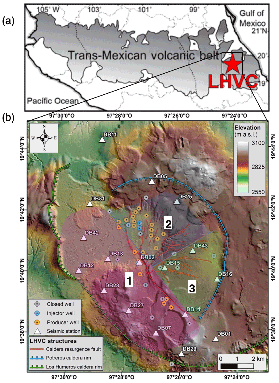
Figure 1 Modified from Norini and Groppelli (2020). (a) Trans-Mexican Volcanic Belt (TMVB), with location of LHVC (Negin and Akbarov, 2019). (b) Volcanotectonic map of the Los Potreros caldera area, being illuminated from the east (on a digital elevation model, DEM). The three key fault zones illuminated and sectioned off as follows: 1 – Maxtaloya–Los Humeros Fault Swarm; 2 – Arroyo Grande Fault Swarm; 3 – Las Papas Fault and parallel faults.

These calderas were formed in the Quaternary during two major caldera-forming phases, some of the LHVC’s many eruptive and intrusion events, which are separated by large Plinian eruptive phases. The first caldera-forming eruption formed a trap door when a collapse occurred unevenly along one side while the opposite side remained with no collapse (Aguirre-Díaz, 2008). This is the Los Humeros caldera. The second eruption produced the Los Potreros caldera (Norini et al., 2019).

The LHVC has inherited local tectonic structures in the basement, which were vital in the evolution of the magma feeding system, caldera collapses and post-caldera deformations (Norini et al., 2019). The collapse of these silicic calderas caused large emissions of pyroclastic material, which triggered the formation of ring faults, displacing the roof of the magma chamber (Norini et al., 2019). The faults' geometry was affected by the shape and depth of the emptying magma reservoir. They could also be controlled by steep discontinuities in the existing crust (Norini et al., 2019). After the collapse, the continuously changing fluid overpressure in the magmatic reservoirs and the related hydrothermal system is what potentially drives the faulting and folding of overlying rocks, which have volcanotectonic deformation, and the resurgence of the caldera floor (Norini et al., 2019). This resurgence of the Los Potreros caldera floor was due to resurgence faults (RFs) (Fig. 1), which were reactivated by the inherited weak planes (Norini et al., 2019). Furthermore, the RFs have dominant known surface directions, the Maxtaloya–Los Humeros Fault swarm having an NNW–SSE strike (which will be depicted as zone 1 in Fig. 1), the Arroyo Grande Fault and parallel faults having a NE–SW strike (zone 2), and the Las Papas Fault swarm having a strike of E–W (zone 3).

It is also important to note the differing lithologies throughout the LHGF, which have different fracture networks due to their differing compositions and formation stages (Norini et al., 2019); furthermore minerals, foliation and preferred crystalline orientation will all have an azimuthal anisotropy response (Cao et al., 2020).

The resurgence faults are vital to the LHGF for the circulation and flow of hydrothermal waters. The seismic anisotropy investigation aims to understand how deeply these faults permeate into the subsurface.

These zones were originally depicted in Rodríguez et al. (2012), where seismic anisotropy of the LHGF using shear waves was collected from seismic events, which gave an indication of the zoning of the fault and/or fracture and stress orientations, where there are three main sectors of particular orientations; this was backed up by findings in Norini et al. (2019). Maxtaloya–Los Humeros Fault swarm has trends parallel to the Mexican Fold and Thrust Belt (MFTB) inherited structures (Norini et al., 2019); the MFTB was generated by the Late Cretaceous–Eocene compressive orogenic phase and has NW–SE-striking folds, although there are some local trend variations which are partially due to the NE–SW regional stress. The MFTB structures can be found in the pre-volcanic sedimentary basement due to the thrusting/folding from the orogenic phase. The sedimentary basement consists of Precambrian–Palaeozoic crystalline rocks, Jurassic and Cretaceous sedimentary rocks, and Eocene–Quaternary intrusive and effusive magmatic rocks (Norini et al., 2019). The basement has fractures, thinly layered carbonates interbedded with cherts and shales, which are affected by outcrop-scale tight chevron folds. The carbonates tend to have an attitude of folding towards the SW. Also, most of the internal deformation of the sediments is displayed by the intense folding, although there are also some intra-formational thrust faults present due to the MFTB (Norini et al., 2019). It is also worth noting the presence of a large anticline fold within the sedimentary and crystalline basement that corresponds to the axis of the MFTB, thus showing the presence of a crystalline metamorphic basement (Teziutlan Massif) within the anticline and below the pre-volcanic sedimentary basement (Norini et al., 2019). Also, there are direct influences of the MFTB on the other lithologies within the stratigraphy of the LHGF, continuing connections with trends in zone 1 throughout the region.

The LHVC is on top of the old volcanic succession and the sedimentary/crystalline basements, respectively.

The LHVC is a Quaternary volcanic complex and is the most prominent silicic volcanic centre within the TMVB. It is a calc-alkaline, andesitic to rhyolite caldera complex (Norini et al., 2015). There is evidence of the presence of monogenetic volcanic centres, which have been emplaced within the caldera complex. They have a spatial distribution defining an NNW–SSE elongated ring-shaped structure; the geometry is parallel to that of the MFTB structures within the LHVC. Further deformation occurred due to the resurgence of the Los Potreros caldera floor, which induced local deformations of the crust (Norini et al., 2019). One of the main resurgent structural sectors is the Maxtaloya–Los Humeros Fault swarm with NNW–SSE trends.

The Arroyo Grande Fault and parallel faults are parallel to the NE–SW regional stress. This regional stress was exerted onto the sedimentary/crystalline basement underlying the TMVB, resulting in the strike of some of the folds generally being NNE–SSW/NE–SW trending (Norini et al., 2019). There are also known Miocene intrusion events of mafic dykes/sills and granite/granodiorite magmatic intrusions along the sub-vertical and vertical planes, which were emplaced within the pre-volcanic sedimentary rocks and are NE–SW trending. There is a low tensile strength of these bedding planes, which allows the propagation of hydraulic fractures driven by excess magma pressure (Gudmundsson, 2011). This occurred during the emplacement of the TMVB magmas, thus driving their trends (Norini et al., 2019). Therefore, corresponding to zone 2, they follow the preferential pathways caused by the Eocene–Pliocene extensional and transtensional phases that produced the N–S- and NE-striking faults (Norini et al., 2015). The deformation caused by this regional stress is also seen in the LHVC. Due to the formation of the LHVC, there is also the possibility of reactivated caldera ring faults caused by the collapse of the trap door Los Humeros Caldera, where the south-eastern sector (zone 2) caldera morphological rim is parallel to the TMVB normal faults, extensional fractures and regional stress (Norini et al., 2019). A weak extensional phase occurred in the LHVC area since the Miocene, with this NE–SW regional stress, which caused the brittle deformation of the crust along the NE–SW-striking normal faults and extensional fractures (Norini et al., 2019). The second main resurgent structural sector is the Arroyo Grande Fault and parallel faults with NE–SW trends.

While zones 1 and 2 have hydrothermal flow depicted due to geothermal production (Fig. 1), zone 3, where the Las Papas structures have a lack of hydrothermal flow, suggests that the E–W-striking structures are shallow with absent or a very weak connection to the geothermal reservoir (Norini et al., 2019).

The mafic dykes/sills and magmatic intrusions tend to be NE–SW trending, thus correlating to zone 2. Due to the different compositions of the LHVC and old volcanic succession lavas and the intrusive lavas, there will be a difference in density and thus Rayleigh wave velocity because of Rayleigh wave dispersion (Telford et al., 1990). When the Rayleigh waves cut across these intrusions, the waves will slow down in comparison to running along the orientation of the mafic dykes/sills because of the difference in density. This distinction is between the intrusive andesites, basalts and rhyodacites, effusive LHVC Teziutlan lavas, which comprises fractured augite andesites (Norini et al., 2015), and the low-permeability silicic post-caldera pyroclastic deposits from the old volcanic succession (Toledo et al., 2020). Andesite is extrusive lava which is of moderate viscosity and is between rhyolite and basalt in terms of composition, whereas basalt is low-viscosity lava. However, they have different silica content: andesite has a higher silica content than basalt (Noble et al., 1975 and Middlemost, 1975). Rhyodacite is more like andesite, as it is an extrusive volcanic rock that is rich in silica (Gillespie and Styles, 1999), whereas the composition of the pyroclastic deposits is transported and reworked volcanic material, thus being clastic rocks composed mainly of volcanic materials (Blatt et al., 2006). Therefore, the seismic anisotropy may be correlating to zone 2 trends of intrusions.

2 Data and methods

2.1 Data

The GEMex project (Toledo et al., 2019) carried out passive seismic monitoring between September 2017 and September 2018 over the LHGF using a multipurpose temporal seismic array. This research, along with any other surveys performed, was part of the framework of the European H2020 and Mexican CONACyTSENER project GEMex (Toledo et al., 2020), which aimed to gain a better understanding of the structures and behaviour of the currently exploited local geothermal system and possible future development sites. The seismic array network comprised 45 3C stations, 25 of which were broadband (BB) stations (22 Trillium C-120s and 3 Trillium C-20 PH) recording at 200 Hz, and 20 of which short-period (SP) stations (Mark L-4C-3D) recording at 100 Hz, and it was sub-divided into two sub-networks. An inner and denser (∼ 1.6–2 km inter-station distance) pseudo-rhomboidal array, consisting of 27 stations, was laid out over the producing zone to retrieve the local seismicity mainly associated with the injection and production operations (Toledo et al., 2019). An outer and sparser array was also developed; however, this array was not used for the 3C beamforming technique. The resulting data that were collected were waveform data and associated metadata, available from the GEOFON data centre under network code 6G (Toledo et al., 2019).

Following Löer et al. (2020), up to 17 stations of the dense broadband (DB) array were used with a frequency sensitivity down to below 0.01 Hz and a sampling rate of 200 Hz. These stations were all centred around the previously located microseismic events within the inner caldera (Löer et al., 2020). The data were pre-processed following Riahi et al. (2013) and Löer et al. (2018); they were downsampled to 10 Hz, bandpass filtered between 0.01–1 Hz, and cleared from linear trends. Spectral whitening and 1 bit normalization were applied in the time domain, normalizing the frequency spectrum and retaining the phase information (Nakata et al., 2019), both of which are necessary for the beamformer whilst absolute amplitudes are not required. A single time window's length corresponds to 4 times the minimum period; this was rounded up to the next power of 2 to speed up Fourier transformation (Löer et al., 2020).

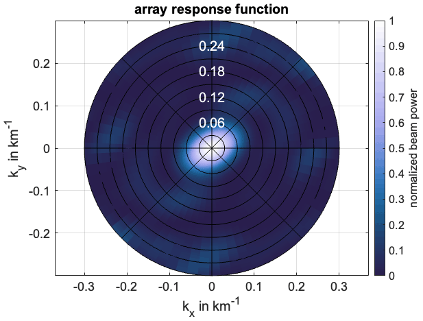
However, not all of these 17 DB stations were used for each day due to a lack of data availability. Only days with eight stations or more were used, resulting in a total of 65 d between 27 October and 30 December 2017; a longer period of time was not used due to computational ability. Over this time range, the sources of ambient noise were some local microseism events, the Caribbean Sea and injection/production activity of the geothermal field. The array can potentially have an effect on the results; however, the array response (Fig. 2) suggests this is not the case and that the array has a minimal effect on the results.

Figure 2 Array response function for the array geometry for 15 of the stations shown in Fig. 1.

2.2 Three-component beamforming

Three-component beamforming is an array method proposed by Riahi et al. (2013) and used here to measure the polarization, phase velocity and azimuth of the seismic noise wavefield as a function of frequency. Therefore, retro- and prograde Rayleigh waves, as well as Love waves, can be identified, as polarization defines the particle movement with respect to the propagation direction (Löer et al., 2018). Love waves have particle movement in the horizontal plane or orthogonal to the propagation direction (Löer et al., 2018), whereas Rayleigh waves are described as being an ellipse in the vertical plane, parallel or antiparallel to the direction of propagation. Therefore, Rayleigh waves are recorded on the vertical and radial components (Riahi et al., 2013). Anisotropy parameters were then fitted to the velocity versus azimuth histograms for both Love and Rayleigh waves.

A bootstrap algorithm (Riahi et al., 2013) was used to evaluate the uncertainty in the fit of these parameters to the histograms that were plotted. These were assessed along with their statistical significance by recomputing the fitting process on bootstrap resamples of data. The bootstrap attempts to estimate the sampling distribution of the actual anisotropy parameters depending on the observed variability in the velocity estimates (Riahi et al., 2013). By starting from N azimuth and phase velocity pairs at a given frequency bin and polarization and randomly sampling (with replacement) an equally large set of N data points, Smith and Dahlen (1973) model parameters are estimated using the fitting method mentioned. This process is then repeated B (number of resamples) times (Riahi et al., 2013). The exact methodology can be found in Appendix A.

The 3C algorithm was later tested using ambient seismic noise to extract information about both isotropic and anisotropic surface wave velocities (Löer et al., 2018). Dispersion curves for Rayleigh and Love waves were computed, and anisotropy parameters were estimated for Love waves; the azimuthal source coverage was too limited to perform anisotropy analysis for Rayleigh waves (Löer et al., 2018).

2.3 Anisotropy curves as a function of depth

Three-component beamforming was performed on ambient seismic noise data recorded on 65 d in 2017. This provided seismic surface wave velocities for retro- and prograde Rayleigh waves as well as Love waves. However, analyses were not done on prograde Rayleigh waves, which are of a higher mode and have a much lower signal compared to Love and retrograde Rayleigh waves, giving a worse source coverage.

The beamforming algorithm was used to detect velocity variations with azimuth in the ambient noise wavefield. The data in the resulting histogram were fitted with an anisotropy curve, as in Riahi et al. (2013) and Löer et al. (2018). More details are provided in the Appendices. The bootstrap resampling was done 1000 times, allowing for a curve to be plotted for each resample in the background of the overall mean anisotropy curve, acting as an uncertainty and improving the reliability of the results. This was plotted as both a histogram with the number of detections conveying the direction of the noise sources and as polar plots to better visualize the fastest directions (fastest velocities' corresponding direction, which was extracted from the anisotropy curves). The direction of propagation is anticlockwise from the east, making an azimuth of 90^∘ equal to north, which was required due to the beamforming method.

Frequency has been related to depth before (Löer et al., 2020) using sensitivity kernels for different wave types obtained using Computer programs in seismology (CPS) surface-wave inversion kernels (surf96) by Herrmann (2013). These kernels indicate the depth that is predominantly sampled by a surface wave at a given frequency. The velocity model from Löer et al. (2020) (shown in Appendices) and CPS was used to produce sensitivity kernels against depth for both Rayleigh and Love waves, thus allowing us to relate differing frequencies of seismic waves to depth (Fig. 3). The depth values were picked where the kernel has half the amplitude of the peak (Rayleigh waves having two such depths and Love waves having one value being the surface), and then the middle of the two depths was taken to be the peak sensitivity for that frequency. The fastest directions were then related to these depths along with the magnitude of apparent anisotropy (a_mag), which indicates how large the variability of the velocity is over the whole range of azimuths. For example, 5 % anisotropy states that the fastest velocity is 5 % larger than the average velocity. Most anisotropy values tend to be below 5 %.

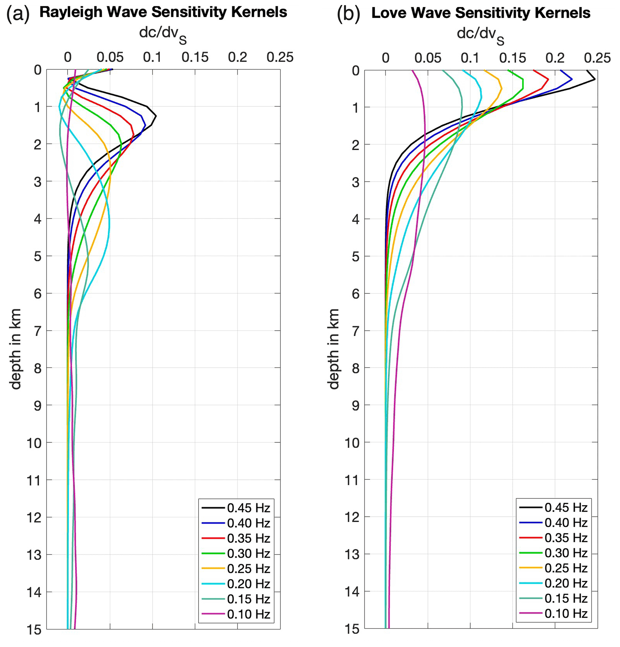
Figure 3 Sensitivity kernels from Computer programs in seismology (Herrmann, 2013) and the velocity model from Löer et al. (2020). (a) Rayleigh wave sensitivity kernels vs. depth. (b) Love wave sensitivity kernels vs. depth.

2.4 Estimating array-induced anisotropy in seismic noise beamforming

We measure velocity versus azimuth in surface wave ambient noise to investigate the azimuthal anisotropy of the subsurface. However, as indicated by Löer et al. (2018) and Lu et al. (2018), for example, these anisotropy measurements can be affected by the geometry of the array used to perform the beamforming analysis.

We use a workflow that estimates the effect of the array geometry on the observed anisotropy by modelling a synthetic, isotropic wavefield in terms of phase shifts corresponding to waves propagating in different directions across the array. Because velocities are isotropic in our model (synthetic wavefield), that is, they do not vary with azimuth, any anisotropy that we observe is a result of the distribution of stations or, in fact, sources. The effect of an uneven source distribution is mitigated by using a large number of time windows, each containing a different normal distribution of sources with a random mean but constant standard deviation as defined in the following. Considering each frequency of interest individually, we superimpose waves travelling in different directions by summing the corresponding phases at each station of the array. The resulting synthetic noise wavefield is then analysed using beamforming, and the detected velocities ($v=f/k$) are plotted against their azimuth in a histogram. This is repeated n = 10 000 times (emulating 10 000 time windows) to populate the histogram sufficiently. Every time, the dominant direction d of the wavefield is chosen randomly from between 0 and 360^∘. We then use a normal distribution of m=90 sources with d as the mean of the distribution and a standard deviation of w=45^∘. All these sources are assumed to act simultaneously in one time window, generating plane waves that superimpose each other at the receiver locations (Fig. 4a).

Figure 4 (a) Example source distribution (red stars) around the Los Humeros stations (black triangles) with the real part of the resulting synthetic wavefield shown in the background. The wavefield is computed in the frequency domain for one frequency; thus there is no time dependency. (b) Beam response obtained for synthetic data shown in (a). The white circle marks the true horizontal wavenumber $k=f/v=\mathrm{0.115}$ km⁻¹.

This synthetic wavefield is analysed following the beamforming method for real data, with the only difference that we consider phase shifts across stations only (not components), like in conventional (1C) beamforming, as these are decisive for measuring horizontal wave velocities across the array (and we are not modelling different wave types simultaneously). More details are provided in Appendix A. For each time window, the maximum of the beam response is extracted (Fig. 4b), converted from wavenumber to velocity and plotted in a histogram that shows velocity as a function of azimuth. The anisotropy curve

$$\begin{array}{}\text{(1)}& \begin{array}{rl}v\left(\mathit{\theta }\right)& =b_{\mathrm{0}}+b_{\mathrm{1}}\cos \left(\mathrm{2}\mathit{\theta }\right)+b_{\mathrm{2}}\sin \left(\mathrm{2}\mathit{\theta }\right)+b_{\mathrm{3}}\cos \left(\mathrm{4}\mathit{\theta }\right)\\ & +b_{\mathrm{4}}\sin \left(\mathrm{4}\mathit{\theta }\right)\end{array}\end{array}$$

(Smith and Dahlen, 1983) is fitted to the histogram (Fig. 5), using least absolute deviation. Because the initial synthetic wavefield model was isotropic, the resulting curve should be flat with b₀ corresponding to the isotropic model velocity and the anisotropy parameters b₁ to b₄ being equal to 0. If these are non-zero, however, and the curve is not flat, apparent anisotropy has been introduced due to the array geometry (or source distribution). The magnitude and fast direction of apparent anisotropy for a given frequency and (isotropic model) velocity can be estimated from the fitted curve. As for the real data, to get an estimate of uncertainty, the histogram is resampled with a bootstrap algorithm B=1000 times, and a curve is fitted to the resampled data. In the end, the mean from all bootstrap curves is taken as an estimate for apparent anisotropy.

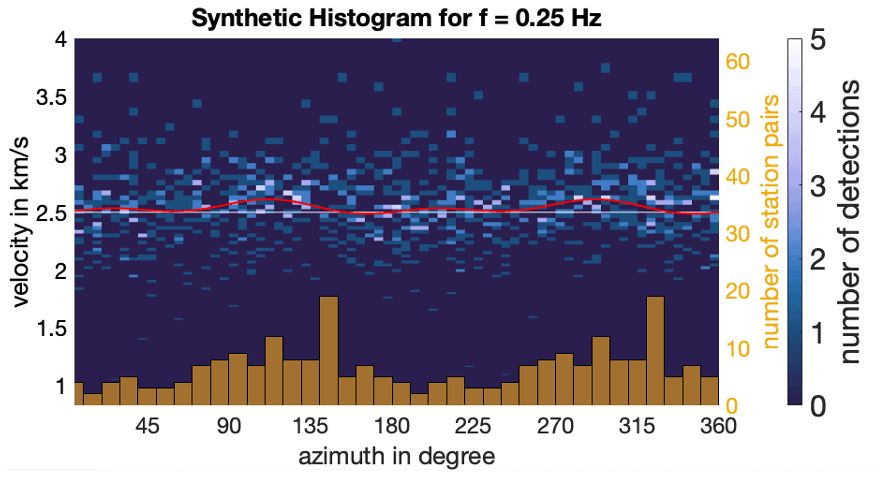
Figure 5 Histogram from synthetic data modelled from 10 000 time windows with fitted anisotropy curves from bootstrap resampling (grey) and the average curve shown in red. Bars on the bottom give the distribution of receiver pair orientations.

We repeat this process for all frequency–velocity pairs obtained from real data histograms to get the apparent anisotropy curve for each such pair. Finally, the anisotropy parameters b₁ to b₄ are subtracted from those found in real data a₁ to a₄ to correct for the effect of the array:

$$\begin{array}{}\text{(2)}& \begin{array}{rl}{v}_{\mathrm{corr}}\left(\mathit{\theta }\right)& =a_{\mathrm{0}}+(a_{\mathrm{1}}-b_{\mathrm{1}})\cos \left(\mathrm{2}\mathit{\theta }\right)+(a_{\mathrm{2}}-b_{\mathrm{2}})\sin \left(\mathrm{2}\mathit{\theta }\right)\\ & +(a_{\mathrm{3}}-b_{\mathrm{3}})\cos \left(\mathrm{4}\mathit{\theta }\right)+(a_{\mathrm{4}}-b_{\mathrm{4}})\sin \left(\mathrm{4}\mathit{\theta }\right)\end{array}\end{array}$$

(Fig. 6).

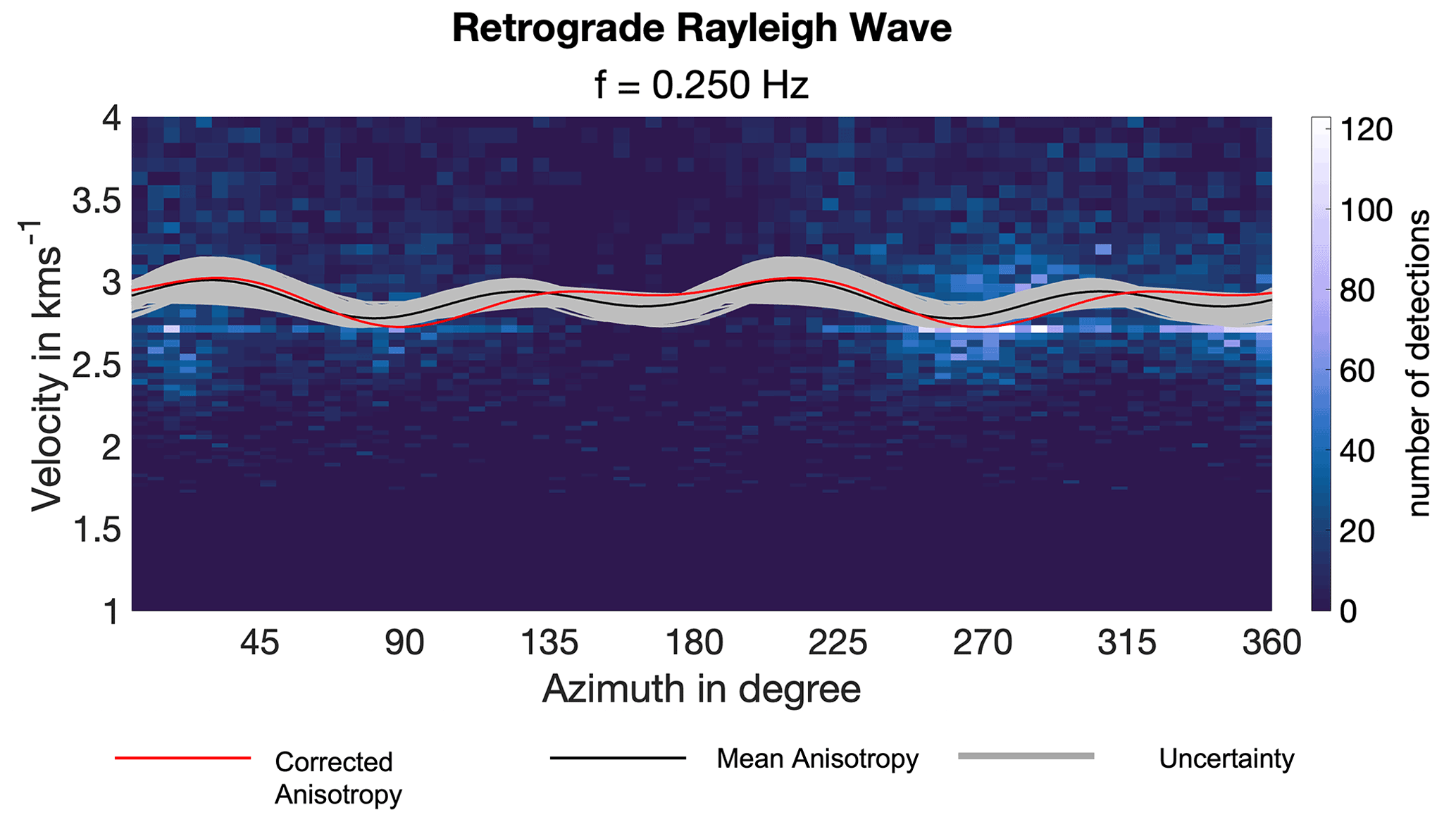
Figure 6 Histogram showing the mean anisotropy (black) of retrograde Rayleigh waves at a frequency of 0.25 Hz, with each resampling of the bootstrap algorithm plotted as a curve (grey) acting as an uncertainty in anisotropy and the corrected anisotropy based on synthetic wavefield (red).

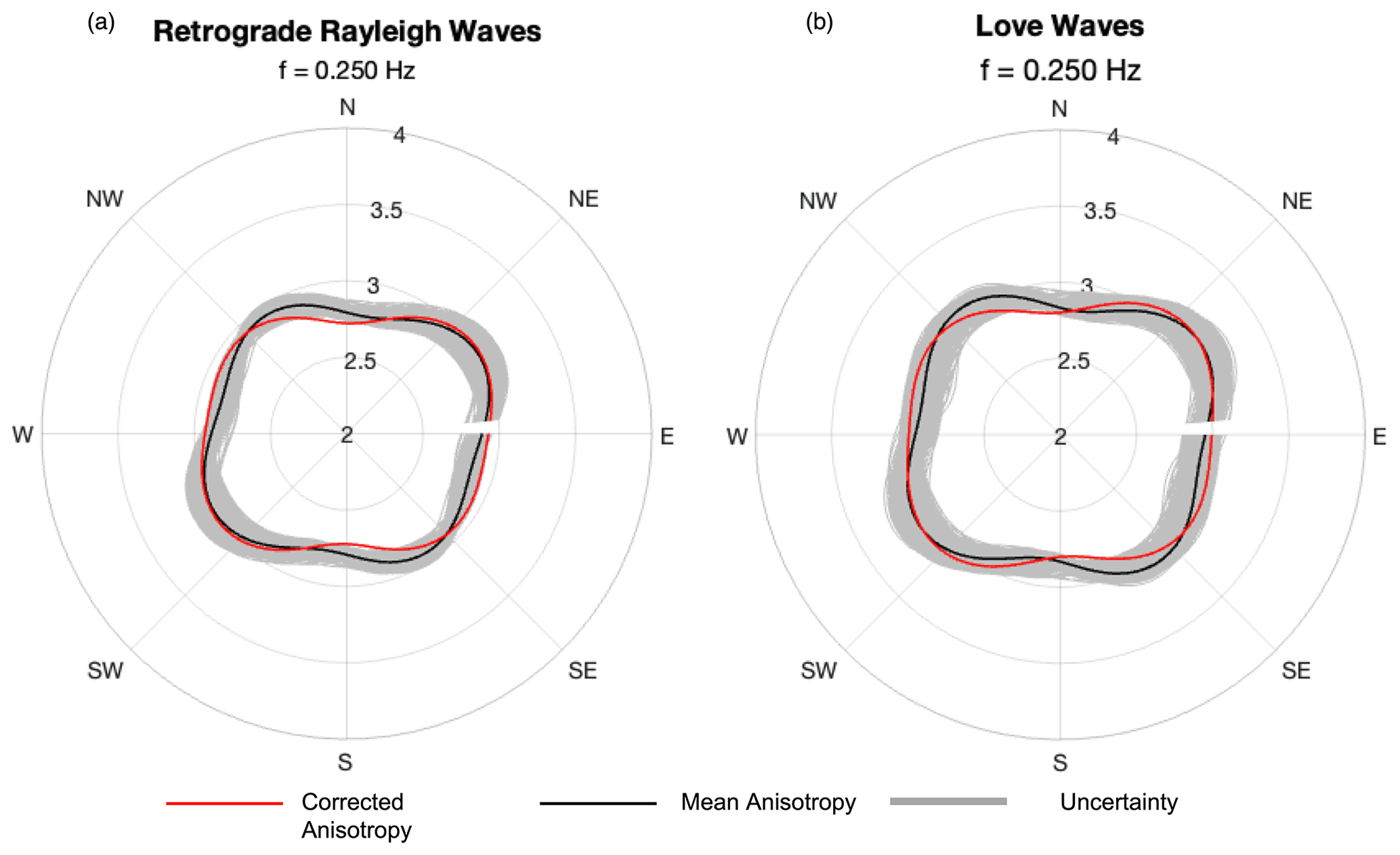
Figure 7 Polar plots of mean anisotropy (black) and anisotropy uncertainty (grey) where the y axis is the velocity. (a) Retrograde Rayleigh waves for a frequency of 0.25 Hz with the corrected curve (red) and mean anisotropy (black). (b) Love waves for 0.25 Hz, with corrected curve and mean anisotropy (black).

3 Results

3.1 Anisotropy with depth

In this study, a frequency range of 0.05 to 0.5 Hz, with a frequency step of 0.05 Hz, was used. The lower limit was chosen due to the spatial aliasing limits of the array, and the upper limit was set to allow for investigation at greater depths, thus not looking at higher frequencies. Hence the following results are only within this frequency range; however, some exclusions were made due to a poor fit between the histogram and the anisotropy, especially at some low frequencies.

The sensitivity kernels for different frequencies of Rayleigh (Fig. 3a) and Love waves (Fig. 3b) show how sensitive the different frequencies are to shear velocity changes at different depths, the peaks being the peak depth sensitivity for that frequency. Rayleigh waves have sensitivity peaks at a significant range of depths, which is likely due to the elliptical particle motion of Rayleigh waves (Haldar, 2018). Referring to Yin et al. (2014), fundamental mode Rayleigh waves tend to perceive information at depths 1.3–1.4 times deeper than Love waves; thus, Love waves are more sensitive to shallower depths than Rayleigh waves (Fig. 3b), which is likely due to the horizontal particle motion of Love waves. Yin et al. (2014) also suggest Love waves should be sensitive at deeper depths than what we perceive from the sensitivity kernels. Therefore, the estimated depth of penetration for Love waves should be assessed with caution.

Because of their larger and better-constrained depth sensitivity, Rayleigh waves are more beneficial for this study and will be the focus of our analysis.

The initial histogram for retrograde Rayleigh waves at a frequency of 0.25 Hz is shown in Fig. 6. The direction of propagation is anticlockwise from the east; 90^∘ is north. Different curves show the mean anisotropy (black), the anisotropy for each resamples of the bootstrap (grey) and the anisotropy corrected for the effect of the array (red). There are minimal changes in the anisotropy curve after correction, decreasing the velocity of two troughs at 120 and 310^∘ and slightly broadening the azimuth of the two fastest directions at 45 and 210^∘, thus making these the clear fastest directions at this frequency. These slight corrections suggest a marginal interference of the array when source distribution is not accounted for.

To better visualize the fast directions, a comparison of the corrected curve, mean anisotropy and uncertainty are shown as polar plots (Fig. 7). The mean anisotropy has been corrected for the array interference (red), whereas the mean anisotropy (black) and the uncertainty (grey) have not been corrected for the effect of the array. It is evident that although the effect of the array is minor, the correction focuses on the fast direction of a Rayleigh wave at a frequency of 0.25 Hz to the NE–SW direction, therefore indicating a potential anisotropic structure at that strike.

The fastest directions for each depth (gained from the sensitivity kernels for the frequencies) for both retrograde Rayleigh and Love waves are shown in Fig. 8. The fastest directions have been corrected (Fig. 8) with respect to the array using the synthetic wavefield that was generated in Sect. 2.4. The black arrows convey the directional of the regional stress acting on the LHVC and thus altering strikes of faults/folds that the fast directions may be corresponding to. The fast directions for Rayleigh waves (Fig. 8a) tend towards the NE–SW strike at depths of 1.5–2.5 km as well as 3.5 km, while depths of Fig. 8b have a similar trend but for shallower depths.

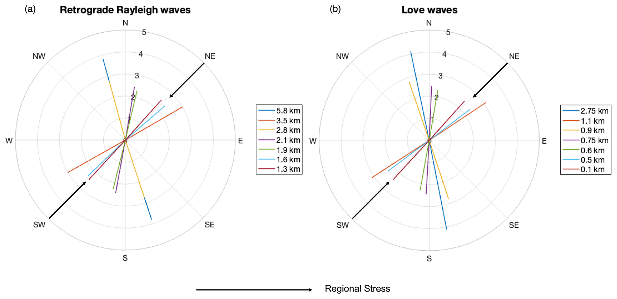
Figure 8 Fastest directions, velocity with respect to orientation, at different depths. The back arrows convey the direction of regional stress. (a) Synthetic correction for retrograde Rayleigh waves. (b) Synthetic correction for Love waves.

The stratigraphy of the LHGF is extremely complex and varies with depth with differing anisotropic signals; thus Fig. 9 shows the fast direction and apparent magnitude at different depths superimposed on the known lithology. Figure 9 focuses on the north-orientated fast directions. There are clear changes in the fastest direction with depth, which also correlates with the changes in magnitude. The fastest directions and apparent magnitude have been corrected for the effect of the array. The clear dramatic shifts in fastest direction, especially for the shallower depths shown by Love waves, may be attributed to the differing known lithologies at varying depths, which will be explored further in the discussion.

Figure 9 Fastest direction (red) and magnitude of apparent anisotropy (black) with depth for (a) retrograde Rayleigh and (b) Love waves; the results have been corrected with synthetic wavefield. The red and black bars depict the area of uncertainty and the shaded areas represent the average depth of the different lithologies using well data from various sources (Arellano et al., 2003; Carrasco-Núñez et al., 2017a, b; Cedillo-Rodríguez, 1997; Norini et al., 2019). The numbers 1 and 2 marked on the graph represent the zone orientation from Fig. 1 that matches the fast directions.

These shifts in fast direction relate to the different zones (1 and 2), which clearly suggests (Fig. 9a) that zone 1 dominant anisotropy permeates to deeper depths than zone 2. However, Fig. 9b also shows a similar pattern of the shallower depths corresponding to zone 2 and the greatest depth matching the orientation of zone 1; this is rather unusual, which causes speculation regarding the reliability of the Love waves results. Nonetheless, there is a greater interest in the deeper depths seen by Rayleigh waves. Consequently, for discussion, analysis of Rayleigh waves will be focused on.

4 Discussion

The LHGF is a geologically complex area with a variety of features impacting surface wave propagation and possibly causing anisotropic behaviour (fault systems, magmatic intrusions, lithology, stress history and hydrothermal flow, among other plausible causations). In our discussion, we try to match our observations with results from other studies focusing on dominant contrasts that are likely to have a strong effect on propagation velocities.

4.1 Limitations

The results were corrected for any potential array effect, which, based on the corrections, had a minimal effect on the fast directions. The correction does not consider the effects introduced by the source distribution of the real data; instead, it assumes a random source distribution (as described in Sect. 2.4) to minimize the effect of sources on the apparent anisotropy. We acknowledge that the source distribution can have a similar effect to the station distribution (Lu et al., 2018), and future work will improve the synthetic wavefield generation and investigate source effects further. The lower frequencies were also not used because of the histograms' lower resolution, thus leading to high uncertainties.

Interpretation of the results assumes the seismic velocity is faster along the orientation of a fault based on the fact that seismic waves will slow down when travelling across boundaries of different material through a fault rather than along it. Another speculation can be linked to different temperature variations within the geothermal field, thus affecting the velocity of the seismic waves; however, this is very speculative. Furthermore, the thermal state of the field is higher along the fault planes within the LHGF (Norini et al., 2019), more specifically, the Maxtaloya–Los Humeros Fault swarm plane (Norini and Groppelli, 2020), thus suggesting the seismic velocity is slower along faults rather than faster. Therefore, the opposite assumption may be made. The thermal state of the field is higher along the fault planes in the Maxtaloya–Los Humeros Fault swarm (Norini et al., 2019), suggesting seismic velocity is slower along faults, so the opposite assumption may be made (Norini and Groppelli, 2020). There is also the potential that the fluid state, the known presence of hydrothermal waters flowing through the fractures, slows down the seismic velocity because of the shear component of Rayleigh and Love waves (Haldar, 2018), contradicting the assumption that seismic waves running along faults are faster (Telford et al., 1990). Testing this hypothesis would require detailed numerical studies, which we aim to address in our future work.

The beamforming method takes the average over the whole area covered by the array. To observe lateral variations, for example, across the three main fault swarm sectors mentioned by Norini et al. (2019) and Rodríguez et al. (2012), it would be both interesting and beneficial to apply beamforming to smaller subarrays in the different sectors. However, these subarrays will suffer from poorer azimuthal and velocity resolution due to smaller apertures and the reduced number of stations. Additionally, there are plans to apply this technique to other geothermally related data sets to further improve the beamforming method and to test the sensitivity of the beamforming method on numerical, anisotropic earth models to better image the geothermal reservoir.

There was a degree of uncertainty when looking at the results for Love waves, as it was originally expected to have a lower phase velocity than Rayleigh waves, yet the results show similar velocities. To investigate this, further theoretical dispersion curves for both Rayleigh and Love waves were computed using the 1-D shear velocity model from Löer et al. (2020) and CPS from Herrmann (2013), using a V_p value of 1.73 for Rayleigh waves, which were then plotted alongside the observed dispersion curves, of 23 d worth of data (Fig. 10). Initially, this was done for lower velocity values in the uppermost crust, using the reference profile from Löer et al. (2020). However, this did not fit the data well; thus higher velocities (maximum likelihood from the inversion of Löer et al., 2020) were used instead (Fig. B1 in Appendix B). This indicates that the velocities in the uppermost crust may be high.

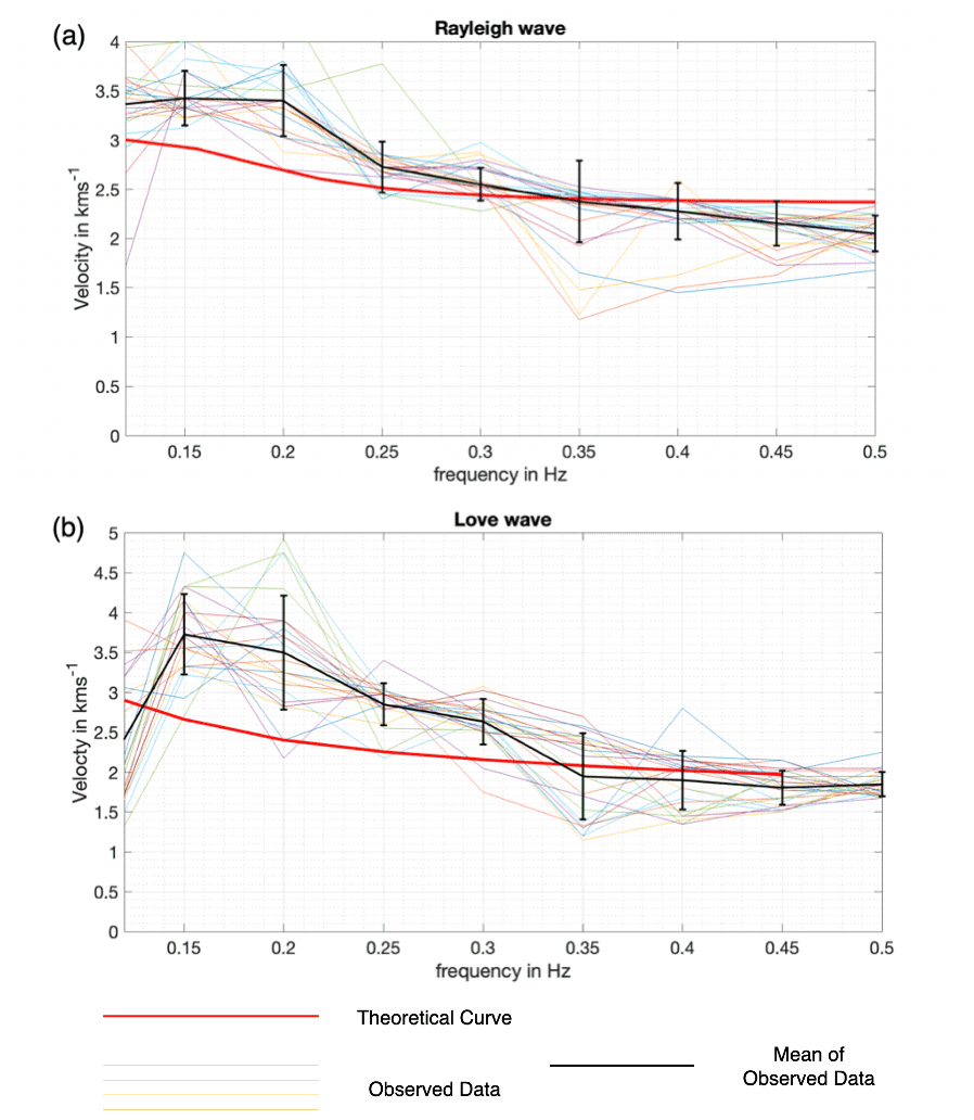
Figure 10 Dispersion curves for (a) Rayleigh waves and (b) Love waves, made using the 1-D velocity model from Löer et al. (2020). Observed dispersion curves (multi-coloured), mean observed curves (black) and theoretical curves (red); black bars represent the degree of error for the real data dispersion curves.

The days that were included for the observed dispersion curves (multi-coloured) were based on what days out of the 65 d used initially had the best source coverage due to a larger number of stations on those days, thus giving more reliable dispersion curves. Meanwhile, some days that did have a large number of stations present were excluded due to erratic fluctuation of velocity at the low frequencies of the surface waves, which did not provide an accurate representation of the dispersion relation between velocity and frequency.

Comparing Fig. 10a and b to each other, the other results agree (to some degree of ambiguity), based on uncertainty (black bars) that the Love waves have, on average, a higher phase velocity than the Rayleigh waves do, thus supporting the fast Love wave velocities shown in the main results. Furthermore, the theoretical dispersion curves (red) for both Fig. 10a and b are within the range (to some extent) of the observed data, having an overall slightly lower phase velocity until a frequency of ∼ 0.34 Hz, where the phase velocity of the red curve crosses over the mean observed data (black line), thus having a higher overall phase velocity for the larger frequencies. This overall pattern of the theoretical curve in comparison to the observed data suggests that the upper crust may be fast, which might explain why the Love waves are so fast overall. However, the synthetic data do not fit the observed data that well; yet, the absolute velocities do not alter the anisotropy results. Hence, this is beyond the scope of this paper.

Nevertheless, it is evident that the degree of uncertainty for Love waves is greater than that of Rayleigh waves, due to the lower number of detections for Love waves. This similarity in velocity further indicates that the depth difference between Rayleigh and love waves is not as large as seen in Fig. 9.

4.2 Fault systems and magmatic intrusions

As the beamforming method takes the average of the whole area, orientations of faults and fractures for the whole LHGF may be detected. The changing fastest directions at varying depths match the orientation of known surface faults in different sectors (Fig. 1b) as mentioned in the section “Background Geology”. Two of these sectors' prominent orientations correspond to the fastest directions at certain depths: zone 1 from 2.8–5.8 km (apart from at 3.5 km) and zone 2 from 0.1–2.8 km, shown in Fig. 9. Rodríguez et al. (2012) also show these sectors. Their shear wave splitting method provides lateral zoning; however, it lacks depth resolution. Using beamforming, we retrieve anisotropy related to depth. Combining this new information with the Rodríguez et al. (2012)/Norini et al. (2019) zones gives us an indication at which depths which fracture orientations are dominant. Figure 9 shows a connection between changes in the fastest direction and changes in lithologies within the LHGF, which (as established earlier) have different fracture networks due to their differing compositions and formation stages, which will affect the azimuthal anisotropy.

Zones 1 and 2 trends can be clearly seen at different depths in Fig. 9, with the trends of the faults parallel to the TMVB normal faults matching the fast directions at shallower depths and the Maxtaloya–Los Humeros Fault swarm trend at deeper depths. The lack of correspondence between the E–W Las Papas structures in the southern resurgent sector coincides with the lack of hydrothermal alterations and geothermal manifestations (Norini et al., 2019). Overall, there is the clear assumption that the anisotropy (azimuthal specifically) shows the trends of the faults. Furthermore, there is a likely correlation between the fast directions and the magmatic intrusions because of their differing compositions/densities to surrounding lavas that are parallel to the TMVB and Mexican Fold and MFTB structures. However, the local variation mentioned, potentially due to the NE–SW regional stress, is feasibly the reason for the zone 2 trending fast direction at 3.5 km in Fig. 9a; or this anisotropy difference is more likely due to a NE–SW-striking intrusion.

Overall, there are clear correlations with the faults in zones 1 and 2 with the fast directions at varying depths, thus indicating the continuation of these faults further below the subsurface.

4.3 Hydrothermal flow and other effects on anisotropy

4.3.1 Effect of (a lack of) hydrothermal flow

Figure 9 conveys that none of the fast directions, after being corrected for the effect for the array, correspond to the fault orientations of the E–W Las Papas Fault swarm. This may be due to a lack of thermal fluid flow that manifests itself in a lack of production in that sector; it can be assumed that the faults in this sector are closed. Overall, this indicates that the anisotropy is sensitive to fault swarms and stress in general but also further sensitive to hydrothermal flow through the faults/fractures. Since seismic wave propagation is sensitive to the presence of water due to the differing density between rock and water, the lack of it in the faults might result in a reduction in anisotropic behaviour. Considering that beamforming estimates the anisotropy averaged over the lateral extent of the array, i.e. over all three zones identified by Rodríguez et al. (2012), the features in the NE and W zone seem to have a dominant effect on the observed wave propagation.

4.3.2 Drilling-induced stresses and fractures

Induced fractures caused by production and injection wells (Fig. 1) usually have similar orientations to major fault systems because of regional stress; however the orientations have altered with depth due to the stress from the wells (Norini et al., 2019). Norini et al. (2019) refer to changes in induced fractures for a geothermal well, where there are clear dynamic changes in the fracture orientation, shifting the orientation by 90^∘ due to stress acting on the fractures by the H43 geothermal well in the north-western sector of the Los Potreros caldera. Therefore induced fractures due to the geothermal wells may affect the overall anisotropy of the field at different depths.

However, it is unusual for induced fractures to change orientation, even due to induced stress from a well, when there is nothing in between the drastically different fracture orientations within the rock. Tingay et al. (2011) looks at drilling-induced fractures where the orientations from most of these wells sharply contrast with the present-day maximum horizontal stresses. Even so, it was found that, unless there was a major mechanical detachment (such as evaporites), the orientation of the fractures would not change drastically. Meanwhile, Norini et al. (2019) presents no evidence of processes that would act as a mechanical detachment horizon; therefore, the only reasoning for the change in fracture orientations attributed to stress could be borehole drilling with greater tensile strength than the rock.

4.3.3 Presence of melt

Another assumption that may be made is that the anisotropy is sensitive to melt; thus the fast directions are indications of said melt due to the differences in rheology (Negin and Akbarov, 2019). Based on mineral–liquid thermobarometry models, Lucci et al. (2020) suggest a magmatic plumbing system comprising multiple shallow magma chambers. Therefore, both models are trying to answer the question of where the heat is feeding the LHGF, which may affect seismic anisotropy due to rheology and thermal state.

However, this model is conceptual and highly schematic. Furthermore, the magmatic intrusions are suggested to be solid and no longer in the form of melt. There is also no clear evidence at present to support the presence of magma chambers at shallow depths as proposed by Lucci et al. (2020); thus, although the presence of melt is conceptually confirmed, information is insufficient to be correlated with observed anisotropy.

4.3.4 Low-velocity zones and $V_{\mathrm{p}}/V_{\mathrm{s}}$ ratio

Low-velocity zones at different depths could be causing anisotropy and hence would be an alternative explanation for what we see in the results. Granados-Chavarría et al. (2022) have shown that the low-velocity zones correspond to the exploited geothermal reservoir itself, thus corresponding to areas of high thermal state and fluid flow. Low-shear-wave-velocity transmission causes these low-velocity zones, which likely correlate to the presence of water (Granados-Chavarría et al., 2022). Therefore, hydrothermal activity is evident in these areas, which may be affecting the anisotropy in the subsurface, bequeathing further exploitation capabilities. The lack of a low-velocity zone in the eastern part (zone 3; Granados-Chavarría et al., 2022) indicates a lack of hydrothermal activity and may thus explain why this area does not produce dominant surface wave anisotropy. Also, Toledo et al. (2020) refers to high-pressure-wave-velocity (V_p) zones which are attributed to these magmatic intrusions (rhyodacitic, andesitic and basaltic volcanic rocks), whereas the low-velocity zones correspond to the pyroclastics deposited in the post-caldera stage. The high $V_{\mathrm{p}}/V_{\mathrm{s}}$ ratio anomalies on each side of the Los Humeros Fault may correspond to hot fluid flow travelling upwards along permeable NNE–SSW faults (Toledo et al., 2020), which in turn are related to the anisotropy we see in the NNE–SSW fast directions (zone 1).

4.3.5 Focal mechanisms

To obtain additional information about fault orientation with depths, we looked at focal mechanisms from earthquakes in 2015 and 2016 that occurred mainly on the Maxtaloya–Los Humeros Fault. The focal mechanisms indicate reverse faulting along planes of rupture with an NNW–SSE strike corresponding to the fast direction of anisotropy observed at larger depths. This reverse slip suggests continuing reverse faulting and compressive stress in the geothermal field (Lermo et al., 2016 and Norini et al., 2019).

4.3.6 Anisotropy on different scales

Although it is reasonable to assume that different sectors are more prominent (permeate further) at certain depths, there is also the chance that the fracturing is not a self-similar process (Ouillon et al., 1995) across all scales. Also, due to smaller frequencies being required in this method to permeate deeper into the subsurface, our resolution decreases in the sense that features are seen at a larger scale (due to the larger wavelength of the low-frequency wave); hence there may be a scale-dependent behaviour at play, giving a different picture of the orientation of the fracture systems at a given greater depth (fractures may be observed as a different orientation than in reality.

5 Conclusions

Matching the results from 3C beamforming with multiple geological studies, we conclude that the most likely explanation for the observed surface wave anisotropy is the presence of continued faults aligned with magmatic intrusions. The fastest directions from the anisotropy correspond to two of the main fault swarm sectors correlating with the area of highest productivity (Maxtaloya–Los Humeros Fault swarm) with a strike of NNW–SSE permeating to depths of >5 km, thus suggesting potential for deeper geothermal production and thus increased longevity of the field. NE–SW fast directions are present at shallower depths of <4 km and correspond to the other zone of high productivity (Arroyo Grande Fault swarm). Fault orientations in a third and less productive sector are not observed in the beamforming analysis. Furthermore, the presence of mafic dykes will contribute to the anisotropy at varying depths, with the same strikes as the two fault swarms that the fast directions correspond to. Especially for a frequency of 0.25 Hz (i.e. the second deepest depth for both surface waves), the observed shift in fast direction corresponding to the Maxtaloya–Los Humeros swarm to the Arroyo Grande Fault swarm may be attributed to these magmatic intrusions.

Our findings support previous suggestions (Löer et al., 2020) that there is no evidence of a brittle–ductile transition at 4 km depth, as there is a clear anisotropic response at depths >4 km.

To obtain a reliable anisotropy signal, various deliberations need to be considered when collecting ambient noise data: array geometry, recording time, ideal source distribution and number of components. We have demonstrated that the array geometry can induce so-called apparent anisotropy and have suggested a workflow to mitigate this problem. While the corrected anisotropy curves were not substantially different to the uncorrected curves, we point out that the effect could be more significant for other array geometries and should thus be considered whenever estimating surface wave anisotropy using seismic noise beamforming. Future work will further optimize the applied correction scheme and, for example, take into account the role of the source distribution. Three-component beamforming is also beneficial as the vertical, north and east components are important to get better dispersion curves/direction of sigma for surface waves, as they are unaffected by body waves. However, while our technique provides an estimate of anisotropy and magnitude and direction, it cannot distinguish directly between different causes of anisotropy and hence requires information from other methods/geology for a meaningful interpretation. Our analysis suggests, however, that certain structures/features have a stronger effect on surface wave velocity compared to others. To examine this relationship in more detail (effectively “calibrate” the method), numerical models are imperative.

Appendix A: Detailed methodology

A1 Three-component beamforming

Three-component beamforming was devised by extending conventional, single-component (vertical) beamforming to additionally decompose polarization for seismic 3C arrays. While conventional beamforming considers the phase shift across different stations of a seismic array, 3C beamforming also accounts for the phase shift across different components of each station, according to the dominant polarization of the wavefield. For a single receiver within the frequency domain, the polarization corresponds to three sinusoids on the 3Cs with differing phases and amplitudes; essentially the three sine curves produced when polarization is considered, which then provides the information for the north, east and vertical components. The polarization parameters (ξ) change depending on the particle motion of the waves, and thus the phase shifts change depending on the polarization parameters. The corresponding phase shifts are shown as c(ξ) (Riahi et al., 2013). These are combined with the array response vector, a(k), which provides phase shifts across stations as a function of the wave vector k, to get the total phase shifts (Eq. A1):

$$\begin{array}{}\text{(A1)}& \mathit{w}(\mathit{k},\mathit{\xi })=\mathit{c}\left(\mathit{\xi }\right)\otimes \mathit{a}\left(\mathit{k}\right),\end{array}$$

with ⊗ denoting the Kronecker product (Riahi et al., 2013). The first elements of w describe the phase responses of the east components, the next elements those of the north components and the final elements those of the vertical components of all stations. The conventional beamforming response function for a three-component case is Eq. (A2) (Riahi et al., 2013):

$$\begin{array}{}\text{(A2)}& R(\mathit{k},\mathit{\xi })=\mathit{w}(\mathit{k},\mathit{\xi })\mathit{†}\cdot \mathrm{S}\mathrm{3}\mathrm{C}\cdot \mathit{w}(\mathit{k},\mathit{\xi }).\end{array}$$

S3C is the cross-spectral density matrix of the data, † represents the transpose and R(k,ξ) is the beamforming response (Riahi et al., 2013). S3C was calculated using the fast Fourier transform (Riahi et al., 2013; Press et al., 2007).

A2 Surface wave azimuthal anisotropy

The surface wave phase velocities were found to vary with azimuth over a wide range of frequencies. This is explained by the anisotropy in the seismic parameters of the subsurface. The surface phase velocity varies due to anisotropy, which is defined in Eq. (A3) and originally defined by Smith and Dahlen (1973).

$$\begin{array}{}\text{(A3)}& \begin{array}{rl}v\left(\mathit{\theta }\right)& =a_{\mathrm{0}}+a_{\mathrm{1}}\cos \left(\mathrm{2}\mathit{\theta }\right)+a_{\mathrm{2}}\sin \left(\mathrm{2}\mathit{\theta }\right)+a_{\mathrm{3}}\cos \left(\mathrm{4}\mathit{\theta }\right)\\ & +a_{\mathrm{4}}\sin \left(\mathrm{4}\mathit{\theta }\right)\end{array}\end{array}$$

v is the phase velocity in kilometres per second, θ is the direction of propagation, which was measured as anticlockwise from the east, and a_i represents the anisotropy parameters that depend on the subsurface. The uncertainty in the anisotropy parameters was then evaluated using bootstrap resamples of the histogram and re-fitting the curve (Sect. 2.2).

A3 Synthetic wavefield

The synthetic frequency domain signal at receiver r_i corresponding to a single source at x_l and wavenumber k_l is given by

$$\begin{array}{}\text{(A4)}& s_i({\mathit{x}}_l,{\mathit{k}}_l)=\exp \mathrm{}\left(i\mathrm{2}\mathit{\pi }\right({\mathit{r}}_i-{\mathit{x}}_l\left){\mathit{k}}_l\right),\end{array}$$

where dependency on frequency has been omitted for brevity. Summing over all sources and wavenumbers provides the final signal at receiver i:

$$\begin{array}{}\text{(A5)}& s_i=\sum _l\exp \mathrm{}\left(i\mathrm{2}\mathit{\pi }\right({\mathit{r}}_i-{\mathit{x}}_l\left){\mathit{k}}_l\right).\end{array}$$

With this synthetic wavefield, we now follow the beamforming algorithm for real data: we compute the cross-spectral density matrix (SDM) S_ij of the synthetic data by cross-correlating (multiplying with complex conjugate in the frequency domain) the data at all stations:

$$\begin{array}{}\text{(A6)}& S_{ij}=s_i\cdot s_j^{*}.\end{array}$$

Looking at S for the case of a single source l=1, it becomes clear that S contains the phase shifts between the stations i and j:

$$\begin{array}{}\text{(A7)}& \begin{array}{rl}{S}_{ij}\left({\mathit{k}}_{\mathrm{1}}\right)& =\exp \mathrm{}\left(i\mathrm{2}\mathit{\pi }\right({\mathit{r}}_i-{\mathit{x}}_i\left){\mathit{k}}_{\mathrm{1}}\right)\cdot \exp \mathrm{}(-i\mathrm{2}\mathit{\pi }({\mathit{r}}_j-{\mathit{x}}_{\mathrm{1}}\left){\mathit{k}}_{\mathrm{1}}\right)\\ & =\exp \mathrm{}\left(i\mathrm{2}\mathit{\pi }\right({\mathit{r}}_i-{\mathit{r}}_j\left){\mathit{k}}_{\mathrm{1}}\right).\end{array}\end{array}$$

The SDM is analysed using the conventional beamforming approach (Riahi et al., 2013), resulting in the beam response for wavenumber k₀ (and frequency ω):

$$\begin{array}{}\text{(A8)}& R\left({\mathit{k}}_{\mathrm{0}}\right)=\mathit{a}({\mathit{k}}_{\mathrm{0}}{)}^{*}\cdot \mathbf{S}\cdot \mathit{a}({\mathit{k}}_{\mathrm{0}}),\end{array}$$

where

$$\begin{array}{}\text{(A9)}& \mathit{a}\left({\mathit{k}}_{\mathrm{0}}\right)={\displaystyle \frac{\mathrm{1}}{\sqrt{n}}}\exp \left(i\mathrm{2}\mathit{\pi }\mathit{r}{\mathit{k}}_{\mathrm{0}}\right)\end{array}$$

is the array response vector as a function of (tested) wavenumber k₀ and the (2×n) vector r contains the station coordinates of all n stations. Note that we only consider phase shifts across stations (not components), like in conventional (1C) beamforming, as these are decisive for measuring horizontal wave velocities across the array.

Appendix B: Additional material

B1 Velocity model

Figure B1 shows the 1-D shear wave velocity model produced in Löer et al. (2020).

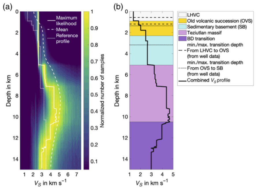
Figure B1 Velocity models used for producing Fig. 3, from Löer et al. (2020). (a) Probability density function (PDF) of shear velocity distribution. (b) Combined shear velocity profile (black) from the analysis of earthquake data (dotted curve in a, down to 3.2 km depth) and ambient noise beamforming.