A functional tool to explore the reliability of micro-earthquake focal mechanism solutions for seismotectonic purposes

Improving the knowledge of seismogenic faults requires the integration of geological, seismological, and geophysical information. Among several analyses, the definition of earthquake focal mechanisms plays an essential role in providing information about the geometry of individual faults and the stress regime acting in a region. Fault plane solutions can be retrieved by several techniques operating in specific magnitude ranges, both in the time and frequency domain and using different data.

For earthquakes of low magnitude, the limited number of available data and their uncertainties can compromise the stability of fault plane solutions. In this work, we propose a useful methodology to evaluate how well a seismic network, used to monitor natural and/or induced micro-seismicity, estimates focal mechanisms as a function of magnitude, location, and kinematics of seismic source and consequently their reliability in defining seismotectonic models. To study the consistency of focal mechanism solutions, we use a Bayesian approach that jointly inverts the P$/$S long-period spectral-level ratios and the P polarities to infer the fault plane solutions. We applied this methodology, by computing synthetic data, to the local seismic network operating in the Campania–Lucania Apennines (southern Italy) aimed to monitor the complex normal fault system activated during the M_s 6.9, 1980 earthquake. We demonstrate that the method we propose is effective and can be adapted for other case studies with a double purpose. It can be a valid tool to design or to test the performance of local seismic networks, and more generally it can be used to assign an absolute uncertainty to focal mechanism solutions fundamental for seismotectonic studies.

1 Introduction

Fault plane solutions represent primary information to describe earthquakes. The assessment of earthquake location, magnitude, and focal mechanism are the fundamental operations to characterize the earthquake source using a point source approximation. The focal mechanism describes the basic geometry and kinematics of a point source in terms of strike, dip, and rake of the fault plane along which the earthquake occurred. So, the focal mechanism is the most important marker of the geometry of the seismogenic faults and their style of faulting. Moreover, seismicity and focal mechanisms of events are often used to constrain seismotectonic models, individual seismogenic sources, the regional strain, and stress fields, also for small magnitudes. Consequently, an evaluation of their effective reliability becomes a fundamental issue in seismotectonic studies.

Nevertheless, focal mechanisms cannot be calculated and constrained every time an earthquake occurs. Although the calculation of focal mechanisms represents a routine analysis for seismological agencies, the solutions are calculated only for a specific range of magnitudes, usually greater than 4. In fact, constraining the solution for earthquakes with small magnitude is still a challenge, despite the advancement in the technological process and the use of increasingly performing seismic networks. This is due to several factors that we will analyse in detail. The techniques used to define the focal mechanism of large to moderate earthquakes are based on the inversion of the moment tensor, which corresponds to a stable and robust procedure, so much that it is the most common method for this type of analysis (Dreger, 2003; Delouis, 2014; Sokos and Zahradnik, 2013; Cesca et al., 2010). This technique requires accurate knowledge of the propagation medium in relation to the range of frequencies used for the modelling waveforms recorded during an earthquake. The smaller an earthquake, the higher the frequency range of the signal to be modelled, the more detailed the knowledge and scale of the Earth's interior must be. Several methods have been proposed to achieve a stable inversion of the moment tensor for earthquakes with a magnitude of less than 3. Hybrid approaches that invert both amplitude and waveform moment tensor use the principal component analysis of seismograms (Vavrycuk et al., 2017) or moment tensor refinement techniques (Kwiatek et al., 2016; Bentz et al., 2018) to facilitate a robust determination of the source type and its kinematics. In particular, the retrieved moment tensor is typically decomposed into volumetric and deviatoric components. Constraining the earthquake as a double-couple source can erroneously affect the retrieved fault plane solutions, especially in the case of induced seismicity where the volumetric or non-double couple component must be considered (Kwiatek et al., 2016).

Other analytical techniques are based on the recognition of the source radiation pattern. According to the position of seismic stations relative to the source, seismic waves on seismograms show different amplitudes and polarities. These features can constrain the geometry of the earthquake faulting through estimating the angular parameters strike, dip, and rake. The classical method (Raesenberg and Oppenheimer, 1985) uses the P-wave polarities; more advanced approaches better constrain the focal mechanism of small earthquakes using P- or S-wave amplitudes or amplitude ratios together with first motions (Snoke, 2003). In fact, the use of polarities alone is inappropriate, especially if we consider micro-seismicity (M<3). The reasons could be the limited number of available data, their uncertainties, and the difficulty of measuring the P polarity with a sufficient degree of precision. For these reasons, different techniques using different types of measurements such as P-wave amplitudes (Julian and Foulger, 1996; Tarantino et al., 2019), P$/$S or S$/$P amplitude ratios measured in the time or the frequency domain (Kisslinger et al., 1981; Rau et al., 1996; Hardebeck and Shearer, 2003; De Matteis et al., 2016), or S-wave polarizations (Zollo and Bernard, 1991) have been developed. The joint inversion of polarities and amplitude ratios led to more stable and robust solutions, allowing us to account for geological site effects and to decrease the effects produced by the geometric and anelastic attenuations.

Two kinds of errors generally influence the goodness of the solution and retrieved model (Michele et al., 2014): the perturbation errors that are related to how the uncertainty on data affects the model, and the resolution errors that are referred to the capability to retrieve a correct model, given a dataset as input or how accurate the model that we can recover could be, even with error-free data. The sum of perturbation and resolution errors corresponds to the final errors on the model obtained by solving an inverse problem, as the solution of the focal mechanism. In particular, the resolution errors depend on the available data and so on the initial condition of the inverse problem. In the case of the focal mechanism, the number of seismic stations, as well as the seismic network geometry, and the velocity structure of the crust influence the resolution and the reliability of the retrieved model.

How will the geometry of a seismic network determine the accuracy of focal mechanism solutions? The answer to this question requires a deep knowledge of the geophysical and geological characteristics of the region, often unavailable. Moreover, the theoretical relationships that predict the focal mechanism solutions for an earthquake scenario could be very complicated if several factors, such as network configuration, noise level, source magnitude, or source kinematics are taken into account. A network configuration may be optimal for earthquake locations but not for retrieving fault plane solutions (Hardt and Scherbaum, 1994). In fact, a given geometry may resolve some fault kinematics better than others.

A seismic network layout is strictly associated with the goals of the network and the available funds; according to these features, a network operator decides how many stations are required and where they should be located (Havskov et al., 2012). So, the number of seismic stations, the size, and geometry of the network are defined after a preliminary phase based on the evaluation of the specific seismological target (Trnkoczy et al., 2009; Hardt and Scherbaum, 1994; Steinberg et al., 1995; Bartal et al., 2000). In the case of small earthquakes, the available recordings come from only a portion of the total network, while the distant stations show a seismic signal buried inside the noise. In order to detect and locate low-magnitude earthquakes, we must increase the number of seismic stations for area units by building a dense seismic network.

In this study, we propose a useful tool to evaluate both (1) the reliability of focal mechanism solutions inferred by the inversion of different seismological data and (2) the performance of the seismic network to assess focal mechanism solutions and their errors. We evaluate the network capability to solve focal mechanisms as a function of magnitude, location, and kinematics of seismic source. We consider three synthetic datasets: P-wave polarities, P- to S-wave amplitude spectral ratios, and polarities and amplitude ratios together. Moreover, different levels of noise are considered in order to simulate more realistic conditions.

As a target, we selected the Irpinia Seismic Network (ISNet), a local seismic network that monitors the Irpinia complex normal fault system (southern Italy), activated during the M_s 6.9 earthquake of 23 November 1980. Evaluating the specific performance of an existing network for a seismological goal is critical and can be used to decide how to improve its layout.

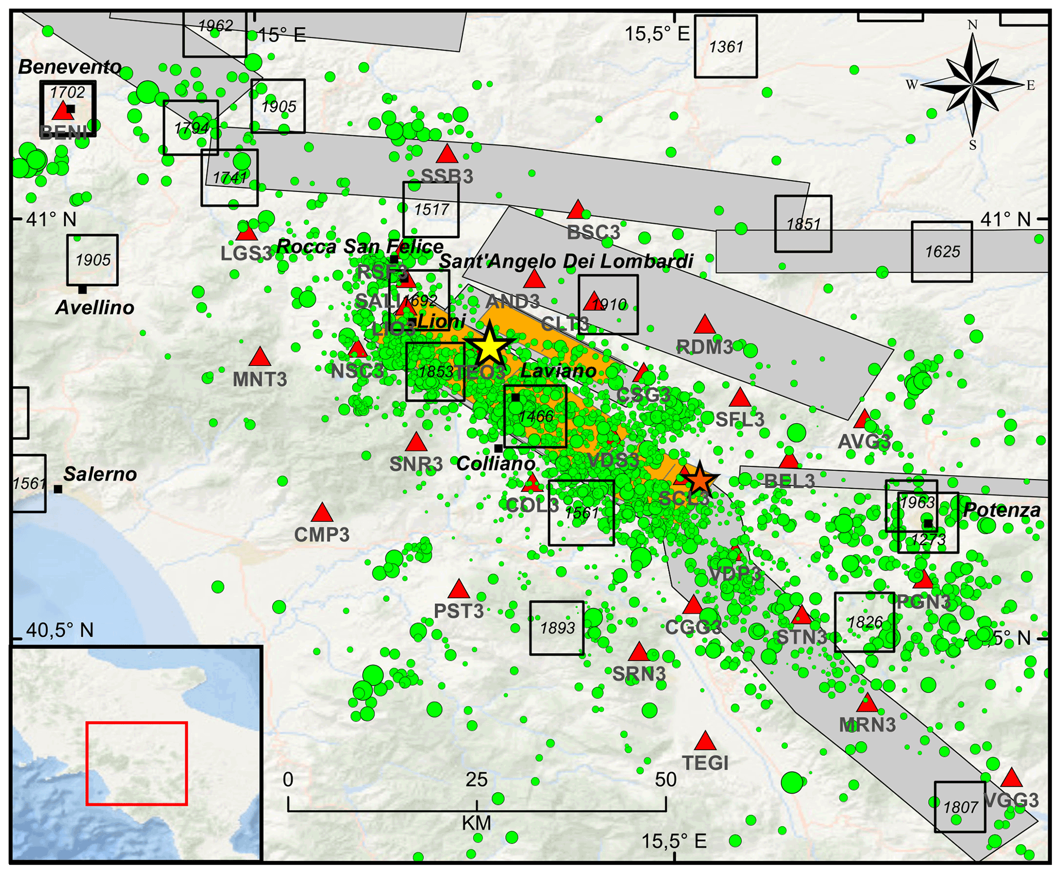
Figure 1 Epicentral map of the earthquakes (green circles) recorded by the Irpinia Seismic Network (ISNet, red triangles) from 2008 to 2020 (http://isnet-bulletin.fisica.unina.it/cgi-bin/isnet-events/isnet.cgi, last access: 1 June 2021). The yellow and orange stars refer to the epicentral location of the 1980, M 6.9 and of the 1996, M 4.9 earthquakes, respectively. Historical seismicity is shown with black squares (I₀ ≥ 6–7 MCS; Mercalli–Cancani–Sieberg). Seismogenic sources related to the Irpinia fault system are indicated by orange rectangles; potential sources for earthquakes larger than M 5.5 in surrounding areas are indicated in grey (Database of Individual Seismogenic Sources, DISS, Version 3.2.1).

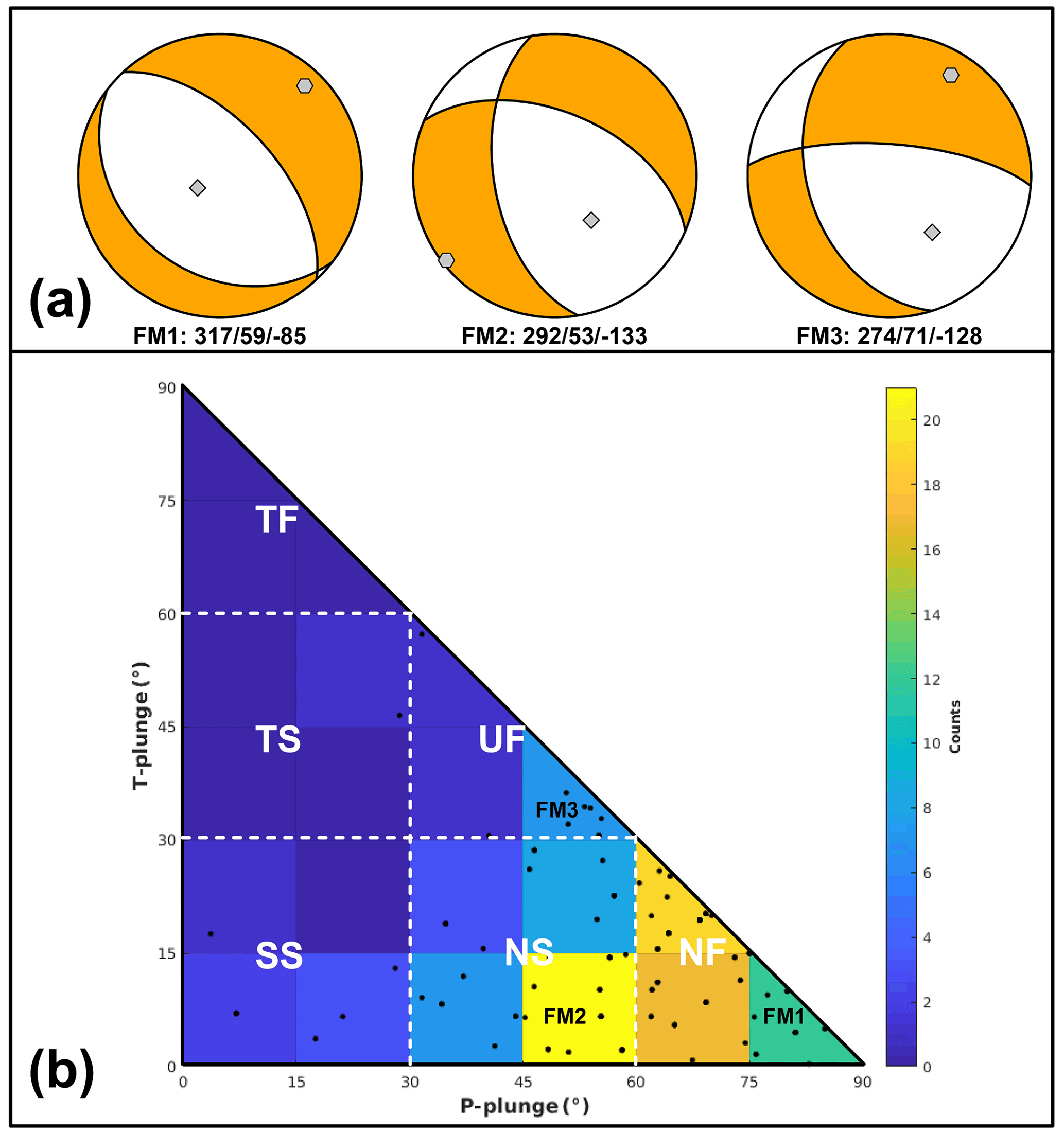
Figure 2 Fault plane solutions used for earthquake simulations. (a) From left to right: (1) M_s 6.9, 23 November 1980 (FM1); (2) and (3) median focal mechanism found from solutions of the first (FM2) and fifth (FM3) most populated bin of histogram of panel (b). (b) Fault plane solutions (black dots) are classified according to the plunge of P- and T axes with the specific tectonic regimes (legend: NF, normal fault; NS, normal strike; SS, strike-slip; TF, thrust; TS, thrust-strike; UF, unknown fault). The number of earthquakes (colour bar) is counted in bins of $\mathrm{15}{}^{\circ }\times \mathrm{15}{}^{\circ }$.

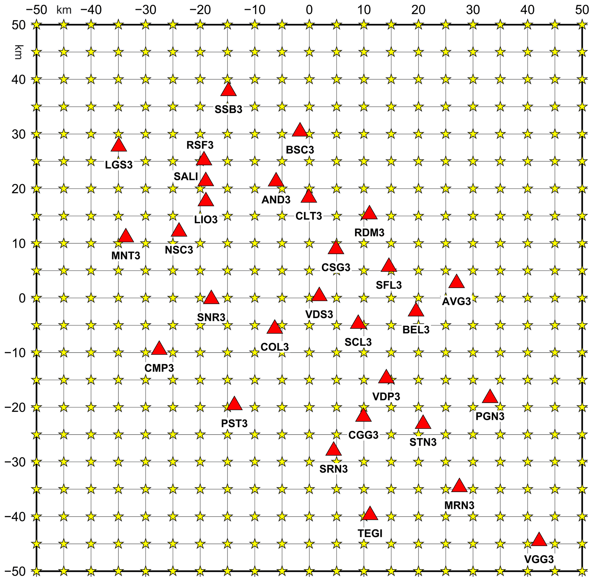
Figure 3 Regular grid of epicentres (yellow stars) used for simulating earthquakes. The area is 100 km×100 km with 5 km of spacing along both horizontal coordinates. The Irpinia Seismic Network (ISNet) is reported with red triangles.

2 Methodology

With the main aim to define the reliability of focal mechanisms retrieved by specific seismic networks, we propose a methodology based on an empirical approach that consists of different steps.

Configuration and parameter tuning (Step 1). In a preliminary phase, we select for each earthquake simulation the (a) fault plane solution to test, (b) seismic observables to be computed (i.e. P-wave polarities or P- to S-wave amplitude spectral ratios), (c) magnitude, (d) the earthquake epicentre and depth, (e) the network geometry, (f) the noise level. The fault plane solution to test can be derived from instrumental seismicity as one of the strongest earthquakes occurred in the area or a median solution of the available ones or simply a fault plane solution representative of the regional seismotectonic. Once the network geometry and the hypocentre of the earthquake are defined, the seismic stations (number and type) for which the synthetic data are computed must be selected. The number of seismic stations that record an event depends on earthquake magnitude, source–station distance, crustal medium properties, and the level of noise. We use an empirical approach, based on the statistical analysis of the local seismicity catalogue that allows us to define, for each magnitude range, a maximum (threshold) epicentral distance for which only the seismic stations within this distance are considered (see “Data analysis” section).

Synthetic data computation (Step 2). Using a crustal velocity model and the source–receiver relative position, the synthetic data are computed for the theoretical fault plane solution. The seismic observables that can be reproduced are (a) P-wave polarities, (b) P$/$S spectral amplitude ratios, and (c) polarities and amplitude ratios together. For the P$/$S spectral level ratios, the Gaussian noise level is added.

Focal mechanism inversion (Step 3). We estimated the focal mechanism using the BISTROP code (De Matteis et al., 2016) that jointly inverts the ratio between the P- and S-wave long-period spectral levels and the P-wave polarities according to a Bayesian approach. BISTROP has the advantage of using different observables for the determination of fault plane solutions, such as the P$/$S long-period spectral level ratios or P-wave polarities, individually or together. The benefits of the use of spectral level ratios are multiple: (1) they can be measured for a broad range of magnitudes (also for M<3; De Matteis et al., 2016); (2) they can be calculated by automatic procedures without visual inspection; (3) their estimates do not require us to identify the first arrival time accurately but only a time window of signal containing P or S phase is mandatory; and (4) the spectral amplitude ratios can generally be used without the exact knowledge of the geological soil conditions (site effects) and geometric and/or anelastic attenuation. Moreover, the joint inversion of amplitude spectral ratios and polarities led to constraining fault plane solutions reducing the error associated with the estimates of retrieved parameters. BISTROP solves an inverse problem through a probabilistic formulation leading to a complete representation of uncertainty and correlation of the inferred parameters.

For a double-couple seismic source, the radiation pattern depends on fault kinematics and relative source–station position. In fact, it can be represented as a function of (1) strike, dip, and rake angles (φ, δ, λ) and (2) take-off and azimuth angles (i_h, φ_r). We can define the ratio between P- and S-wave radiation pattern coefficients as

$$\begin{array}{}\text{(1)}& {\displaystyle \frac{{\mathcal{R}}^{\mathrm{P}}(\mathit{\varphi },\mathit{\delta },\mathit{\lambda },i_{\mathrm{h}},{\mathit{\varphi }}_{\mathrm{R}})}{{\mathcal{R}}^{\mathrm{S}}(\mathit{\varphi },\mathit{\delta },\mathit{\lambda },i_{\mathrm{h}},{\mathit{\varphi }}_{\mathrm{R}})}}=\left({\displaystyle \frac{{\mathit{\alpha }}_{\mathrm{s}}^{\mathrm{2}}{\mathit{\alpha }}_{\mathrm{r}}}{{\mathit{\beta }}_{\mathrm{s}}^{\mathrm{2}}{\mathit{\beta }}_{\mathrm{r}}}}\right){\displaystyle \frac{{\mathrm{\Omega }}_{\mathrm{0}}^{\mathrm{P}}}{{\mathrm{\Omega }}_{\mathrm{0}}^{\mathrm{S}}}},\end{array}$$

where ${\mathrm{\Omega }}_{\mathrm{0}}^{\mathrm{P}}$ and ${\mathrm{\Omega }}_{\mathrm{0}}^{\mathrm{S}}$ are the long-period spectral level of the P and S waves, respectively, and α_s, α_r, β_s, β_r, are the P- and S-wave velocities at the source and at the receiver, respectively. Thus, using the displacement spectra, assuming a given source and attenuation model (Boatwright, 1980), we can derive from the signal recorded by a seismic station the ratio of radiation pattern coefficients for P and S phases, and α, β, i_h, and φ_r are known from the earthquake location and the velocity model used. So, from a theoretical point of view, the spectral amplitude ratios measured at several seismic stations can be used to retrieve the ratio of radiation pattern coefficients ${\mathcal{R}}_{\mathit{\theta }\mathit{\phi }}^{\mathrm{P}}/{\mathcal{R}}_{\mathit{\theta }\mathit{\phi }}^{\mathrm{S}}$ as a function of the source–receiver azimuth and take-off angles.

BISTROP jointly inverts the spectral amplitude ratios with the observed P-wave polarities to infer the parameters φ, δ, and λ of the focal mechanism in a Bayesian framework. A posterior probability density function (PDF) for the vector of model parameter m (φ, δ, λ) and the vector of observed data d is defined as

$$\begin{array}{}\text{(2)}& q\left(\mathit{m}\mathrm{|}\mathit{d}\right)={\displaystyle \frac{f\left(\mathit{d}\mathrm{|}\mathit{m}\right)p\left(\mathit{m}\right)}{{\int }_{M}f\left(\mathit{d}\mathrm{|}{\mathit{m}}^{\prime }\right)p\left({\mathit{m}}^{\prime }\right)d{\mathit{m}}^{\prime }}},\end{array}$$

where f(d|m) is the conditional probability function that represents the PDF given the data d and for parameter vector m in the model parameter space M, and p(m) is the a priori PDF. If P-wave polarities and P$/$S spectral level ratios are independent datasets, the conditional probability function may be written as

$$\begin{array}{}\text{(3)}& f\left(\mathit{d}\mathrm{|}\mathit{m}\right)=f\left({\mathit{d}}^{\mathrm{L}}\mathrm{|}\mathit{m}\right)f\left({\mathit{d}}^{\mathrm{P}}\mathrm{|}\mathit{m}\right),\end{array}$$

in which the PDF of the data vector d^L of N^L measurements of spectral ratios is multiplied for the PDF of data vector d^P of N^P measurements of P-wave polarities given the model m.

Assuming that the observables have the same finite variance, for the N^L observations of spectral level ratios the conditional probability function may be defined as

$$\begin{array}{}\text{(4)}& f\left({\mathit{d}}^{\mathrm{L}}\mathrm{|}\mathit{m}\right)={\displaystyle \frac{\mathrm{1}}{(\sqrt{\mathrm{2}\mathit{\pi }}\mathit{\sigma }{)}^{N_{\mathrm{L}}}}}\exp \left(-{\displaystyle \frac{{\sum }_{i=\mathrm{1}}^{N_{\mathrm{L}}}\mathit{\{}{d}_i-[G\left(\mathit{m}\right){]}_i{\mathit{\}}}^{\mathrm{2}}}{\mathrm{2}{\mathit{\sigma }}^{\mathrm{2}}}}\right),\end{array}$$

where G(m) represents a functional relationship between model and data and corresponds to Eq. (1) and σ represents the uncertainty on the spectral measure.

For the N^P observations of P-wave polarities, the conditional probability function is (Brillinger et al., 1980)

$$\begin{array}{}\text{(5)}& f\left({\mathit{d}}^{\mathrm{P}}\mathrm{|}\mathit{m}\right)=\prod _{i=\mathrm{1}}^{N_{\mathrm{P}}}{\displaystyle \frac{\mathrm{1}}{\mathrm{2}}}\left[\mathrm{1}+\mathit{\psi }\left({\mathcal{R}}_i^{\mathrm{P}},{\mathit{\gamma }}_i,{\mathit{\rho }}_{\mathrm{0}}\right)Y_i\text{sign}\left({\mathcal{R}}_i^{\mathrm{P}}\right)\right],\end{array}$$

in which

$$\begin{array}{}\text{(6)}& \mathit{\psi }({\mathcal{R}}_i^{\mathrm{P}},{\mathit{\gamma }}_i,{\mathit{\rho }}_{\mathrm{0}})=\left(\mathrm{1}-\mathrm{2}{\mathit{\gamma }}_i\right)\text{erf}\left(\right|{\mathit{\rho }}_{\mathrm{0}}{\mathcal{R}}_i^{\mathrm{P}}\left(\mathit{m}\right)\left|\right).\end{array}$$

The quantity reported in square brackets in Eq. (5) represents the probability that the observed ith polarity γ_i is consistent with the theoretical one computed from the model m, whose theoretical P-wave amplitude is ${\mathcal{R}}_i^{\mathrm{P}}$ and $\text{sign}\left({\mathcal{R}}_i^{\mathrm{P}}\right)$ is its polarity at the ith station for a given fault plane solution. The parameters ρ_s and γ₀, referring to the errors in ray tracing due to velocity model ambiguity and to the uncertainty in polarity reading, regulate the shape of the PDF. For more details about the mathematical formulation, see De Matteis et al. (2016).

Evaluation of the results (Step 4). Once the best solution is estimated, the focal mechanism uncertainties and its misfit, with respect to the theoretical solution as Kagan angle, are computed. The focal mechanism parameter (strike, dip, and rake) misfit and parameter uncertainties are also calculated.

3 Irpinia Seismic Network

As a test case for our methodology, we choose the area of the M 6.9, 1980 Irpinia earthquake (southern Italy). Since 2005, ISNet, a local, dense seismic network, monitors the seismicity along the Campania–Lucania Apennines covering an area of about 100 km×70 km (Fig. 1; Weber et al., 2007). The seismic stations are deployed within an elliptic area whose major axis, parallel to the Apennine chain, has a NW–SE trend with an average inter-station distance of 15 km that reaches 10 km in the inner central zone. Each seismic station ensures a high dynamic range and is equipped with a strong-motion accelerometer (Guralp CMG-5T or Kinemetrics Episensor) and a short-period three-component seismometer (Geotech S13-J) with a natural period of 1 s. In six cases, broadband seismometers are installed such as the Nanometrics Trillium with a flat response in the range 0.025–50 Hz. ISNet is operated by INFO (Irpinia Near Fault Observatory) and it provides real-time data at local control centres for earthquake early warning systems or real-time seismic monitoring (Satriano et al., 2011). Seismic events are automatically identified and located from continuous recordings by automatic Earth-worm Binder (Dietz, 2002) and data are then manually revised by operators (Festa et al., 2021).

The 1980, M 6.9 Irpinia earthquake was one of the most destructive, instrumental earthquakes of the Southern Apennines, causing about 3000 fatalities and severe damage in the Campania and Basilicata regions. It activated a NW–SE-trending normal fault system with a complex rupture process involving multiple fault segments according to (at least) three different nucleation episodes each delayed by 20 s (Bernard and Zollo, 1989; Pantosti and Valensise, 1990; Amoruso et al., 2005). No large earthquakes have occurred in the Irpinia region since 1980. A M_w 4.9 earthquake took place in 1996 causing a seismic sequence inside the epicentral area of the 1980 earthquake (Fig. 1; Cocco et al., 1999). Recent instrumental seismicity occurs mainly in the first 15 km of the crust showing fault plane solutions with normal and normal strike-slip kinematics, indicating a dominant SW–NE extensional regime (Pasquale et al., 2009; De Matteis et al., 2012; Bello et al., 2021). Low-magnitude seismicity (M_L<3.6) is spread into a large volume related to the activity of major fault segments of the 1980 Irpinia earthquake (Fig. 1; Adinolfi et al., 2019, 2020). Seismic sequences or swarms often occurred in the area, extremely clustered in time (from several hours to a few days) and space and seem to be controlled by high pore fluid pressure of saturated Apulian carbonates bounded by normal seismogenic faults (Stabile et al., 2012; Amoroso et al., 2014).

Figure 4 KAM (Kagan angle misfit) map for retrieved focal mechanisms with the D1 dataset as input data and simulating earthquakes with M3 magnitude and FM1 (a), FM2 (b), and FM3 (c) theoretical fault plane solutions at 10 km depth.

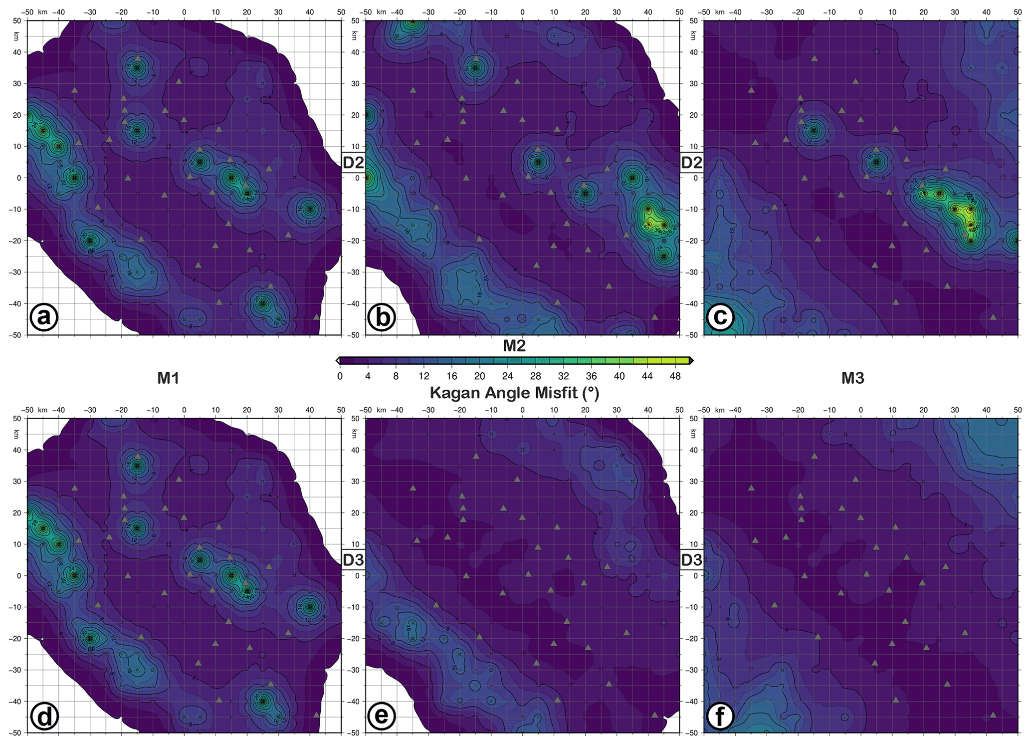
Figure 5 KAM (Kagan angle misfit) map for retrieved focal mechanisms with D2 (a–c) and D3 (d–f) datasets as input data and simulating earthquakes with M1 (a, d), M2 (b, e), and M3 (c, f) magnitudes and the FM1 theoretical fault plane solution at 10 km depth. The level of Gaussian noise is set to 5 %.

4 Data analysis

We applied the method we proposed and evaluated the capability of the ISNet local network to resolve fault plane solutions using different observables as input data: (a) P-wave polarities, (b) P$/$S spectral amplitude ratios, and (c) polarities and amplitude ratios together. The analysis is carried out by evaluating the effect of (1) earthquake magnitude, (2) epicentral location, (3) earthquake depth, (4) signal-to-noise ratio, and (5) fault kinematics on retrieved focal solutions as previously described.

Step 1. In order to select focal mechanisms (FMs) to be used for our resolution study (Fig. 2a), we carried out statistical analysis to define the most frequent fault plane solutions of instrumental seismicity. According to the plunge of P and T axes, we classified the fault plane solutions reported in De Matteis et al. (2012) choosing only the FMs occurring within the Irpinia area since 2005 to 2011. As shown in Fig. 2b, splitting the range of the data into equal-sized bins, we selected the focal mechanism corresponding to the median value of the most populated class. We report it in Fig. 2a as FM2. This corresponds to a normal strike-slip fault plane solution with strike, dip, and rake equal to 292, 53, and −133^∘, respectively. Then, we decided to test the focal mechanism solution of the1980 Irpinia earthquake, a pure normal fault (strike, dip, rake: 317, 59, $-\mathrm{85}{}^{\circ }$; Westaway and Jackson, 1987; Fig. 2a) here and after FM1. This solution is very similar to the focal mechanism corresponding to (1) the regional stress field (see Supplement), (2) the M_L 2.9 Laviano earthquake, one of the most energetic earthquakes of the last years (Stabile et al.; 2012), and (3) those of the second, third, and fourth most populated bins. Finally, we selected the solution corresponding to the fifth bin reported as FM3 in Fig. 2a. This focal mechanism is quite different from the others due to a predominant component along the fault strike (strike, dip, rake: 274, 71, $-\mathrm{128}{}^{\circ }$).

Step 2. For each of the three selected fault plane kinematics, we calculated synthetic data (P-wave polarities or P- and S-wave spectral amplitudes) at seismic stations varying the earthquake location and by using a local velocity model (Matrullo et al., 2013). We discretize the study area with a square grid (100 km×100 km), centred on the barycentre of ISNet, with 441 nodes and a sampling step of 5 km. Each node corresponds to a possible earthquake epicentre (Fig. 3).

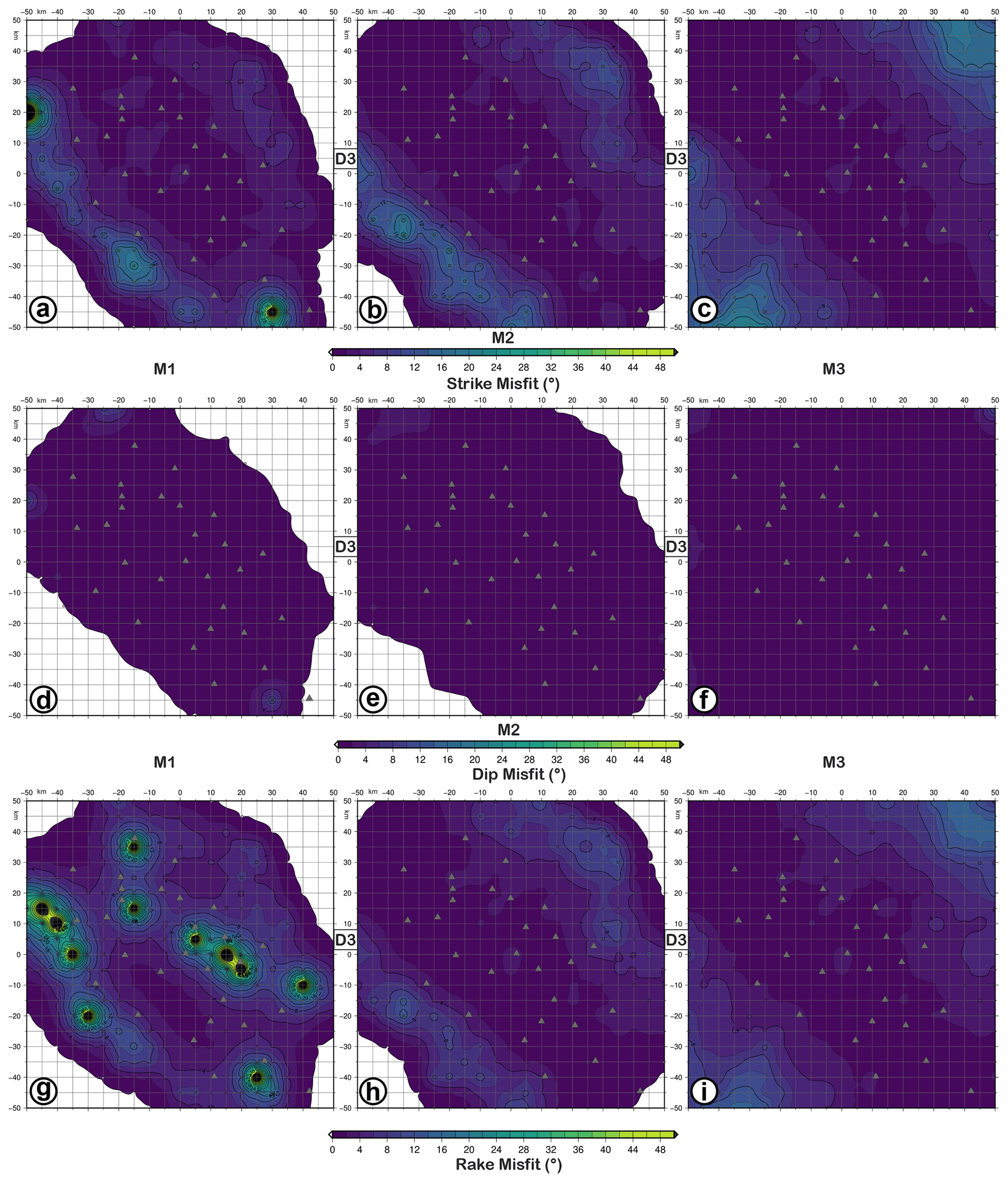
Figure 6 FMM (focal mechanism parameter misfit) maps for retrieved focal mechanisms with D3 datasets as input data and simulating earthquakes with M1 (a, d, g), M2 (b, e, h), and M3 (c, f, i) magnitudes and the FM1 theoretical fault plane solution at 10 km depth. Panels (a–c) refer to strike misfit; (d–f) refer to dip misfit; (g–i) refer to rake. The level of Gaussian noise is set to 5 %.

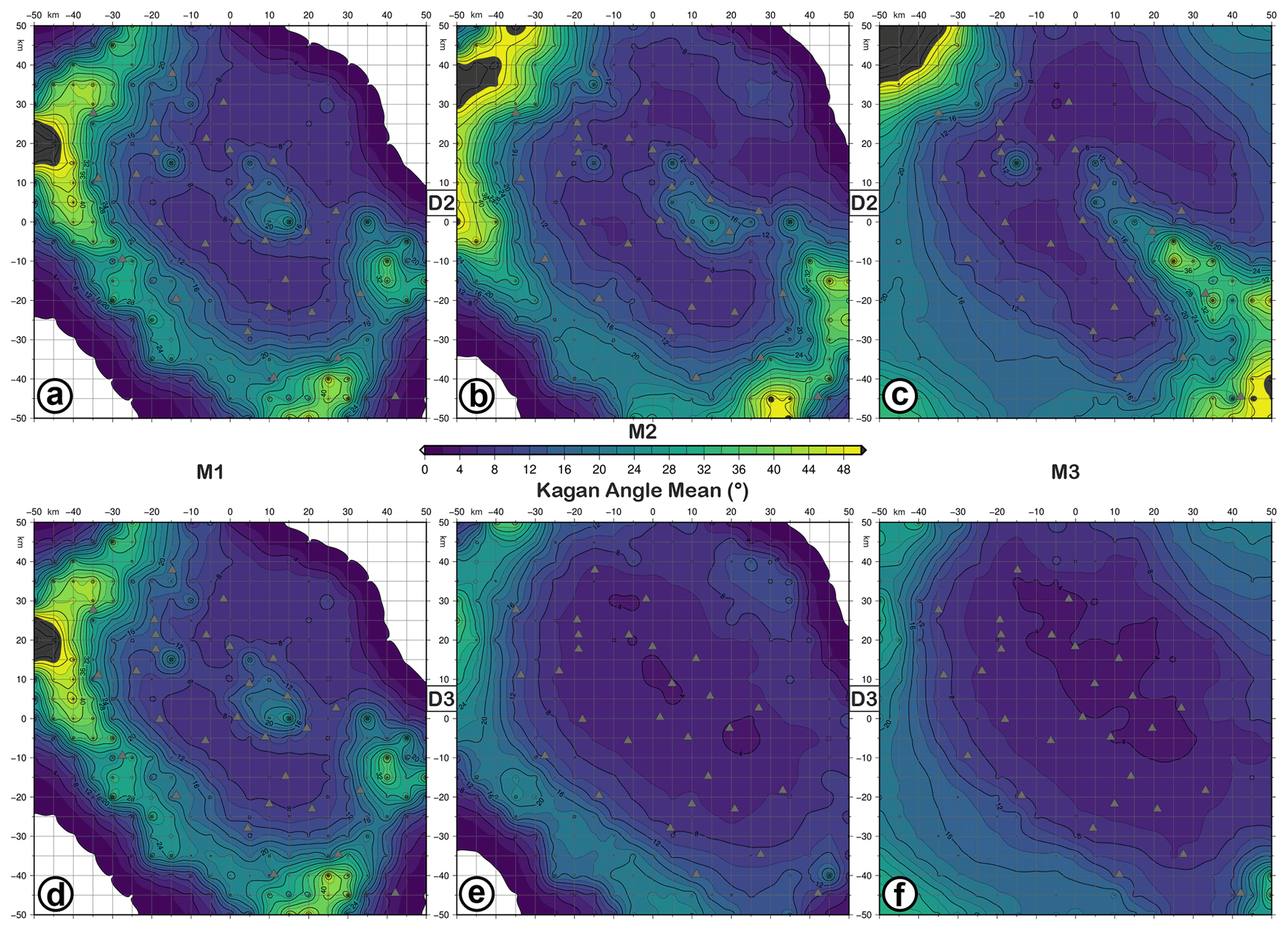
Figure 7 KAA (Kagan angle average) maps for retrieved focal mechanisms with D2 (a–c) and D3 (d–f) datasets as input data and simulating earthquakes with M1 (a, d), M2 (b, e), and M3 (c, f) magnitudes and the FM1 theoretical fault plane solution at 10 km depth. The level of Gaussian noise is set to 5 %.

For each grid node and according to the earthquake magnitude to be tested, we have to select the ISNet stations for simulations. The number of seismic stations that record an event depends on earthquake magnitude, source–station distance, crustal medium properties, and the noise level. Theoretical relationships that link the seismic source to the signal recorded at every single station are quite complicated (Kwiatek et al., 2016, 2020) and are based on the accurate knowledge of crustal volumes in which the seismic waves propagated, such as the three-dimensional wave velocity structure, anelastic attenuation, and/or site conditions of a single receiver. To overcome this limitation, we used an empirical approach to define the number and the distance of the seismic stations that record a seismic signal as a function of magnitude, once its epicentral location (grid node) and depth are fixed. Using the bulletin data retrieved by INFO at ISNet during the last 2 years (January 2019–March 2021; http://isnet-bulletin.fisica.unina.it/cgi-bin/isnet-events/isnet.cgi, last access: 1 June 2021), we selected two earthquake catalogue datasets with depths equal to 5 (±2) and 10 (±2) km, respectively, and local magnitude ranging between 1.0 and 2.5. These choices are motivated by the characteristics of the Irpinia micro-seismicity recorded by ISNet. Then, we divided each dataset into bins of 0.5 magnitudes, and for each bin, we retrieved the median number of P-wave polarity readings and the median epicentral distance of the farthest station that recorded the earthquake (Table 1). The bulletin data are manually revised by operators, and we selected only seismic records that provide P- and/or S-wave arrival times. The median value of the distance of the farthest station is then used to select the seismic stations for which synthetic data are calculated. Therefore, for each earthquake simulation of a specific magnitude and depth, only the seismic stations with a distance from the grid node under examination (epicentre) equal or lower than the maximum distance, reported in Table 1, are considered. We run simulations only for earthquakes recorded at least by six seismic stations. The synthetic P-wave polarities are simulated only at a number of stations corresponding to the median value previously defined. (Table 1). We pointed out that the number of P-wave polarities empirically assigned is related to the available earthquake catalogue data of the Irpinia region where the seismicity can occur in different portions of the area covered by the network, not always with optimal azimuthal coverage.

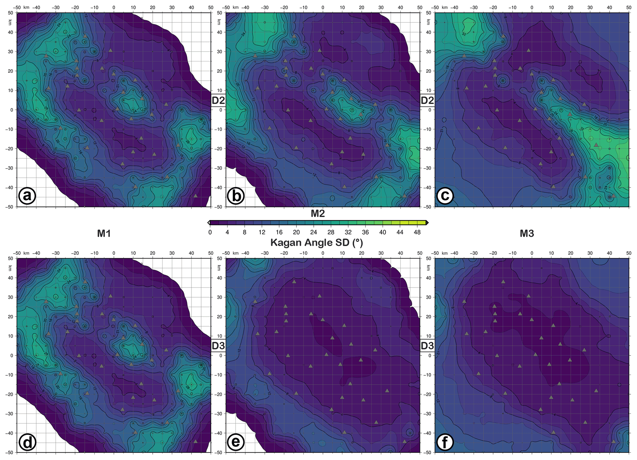
Figure 8 KAS (Kagan angle standard deviation) maps for retrieved focal mechanisms with D2 (a–c) and D3 (d–f) datasets as input data and simulating earthquakes with M1 (a, d), M2 (b, e), and M3 (c, f) magnitudes and the FM1 theoretical fault plane solution at 10 km depth. The level of Gaussian noise is set to 5 %.

Table 1 Maximum distance of the farthest triggered seismic station and number of P-wave polarities as function of earthquake magnitude and depth. The values, empirically derived from the ISNet bulletin, are used for the earthquake simulations.

Additionally, we simulated the uncertainty on the measure of spectral level ratios or the effect of seismic noise adding a zero mean, Gaussian noise to the synthetic data with a standard deviation equal to two different percentage levels, as 5 % and 30 %. With this configuration, we simulated

• three datasets of seismic observables: P-wave polarities (D1), P$/$S spectral level ratios (D2), and polarities and P$/$S spectral level ratios together (D3);

• two hypocentre depths: 5 and 10 km;

• three magnitude bins: M_L 1.0–1.5 (M1), M_L 1.5–2.0 (M2), and M_L 2.0–2.5 (M3);

• three focal mechanism solutions: FM1 (317, 59, $-\mathrm{85}{}^{\circ }$), FM2 (292, 53, $-\mathrm{133}{}^{\circ }$), and FM3 (274, 71, $-\mathrm{128}{}^{\circ }$).

The two levels of Gaussian noise are 5 % and 30 %. When D2 is simulated, in order to solve the verse ambiguity of the slip vector, a P-wave polarity is added to the earthquake data to be inverted for the focal mechanism.

Step 3. For each earthquake simulation the focal mechanism was estimated by inverting the synthetic data with BISTROP (De Matteis et al., 2016).

Table 2 Summary of the Figs. 4–12 with parameters used for earthquake simulations whose results are represented as a specific map.

Step 4. In order to analyse the results, we defined five kinds of map to study how the FM resolution and error spatially change in the area where ISNet is installed (Table 2):

• Kagan angle misfit map (KAM)

• map of the focal mechanism parameter misfit (FMM)

• strike, dip, and rake error map (FME)

• Kagan angle average map (KAA)

• Kagan angle standard deviation map (KAS).

The Kagan angle (KA) measures the difference between the orientations of two seismic moment tensors or two double couples. It is the smallest angle needed to rotate the principal axes of one moment tensor to the corresponding principal axes of the other (Kagan et al., 1991; Tape and Tape, 2012). The smaller the KA between two focal mechanisms, the more similar they are. In the KAM map, for each node the value of KA between the theoretical and retrieved solution is reported, while in the FMM map, the absolute value of the misfit between the strike, dip, and rake angles of the retrieved and theoretical solution is indicated. FME is defined as the error map of strike, dip, and rake in which the uncertainties (standard deviations) are calculated considering all the solutions with a probability larger than the 90 % (S90) of the maximum probability, corresponding to the best solution retrieved. Additionally, these solutions are used to study how constrained the FM solution is. The KA is calculated between each FM of S90 solutions and the retrieved best solution. The mean and the standard deviation of the resulting KA distribution are plotted in the KAA and KAS maps, respectively. The smaller the KA mean and standard deviation (SD), the more constrained the obtained fault plane solution is (Table 2).

Table 3 Fault plane solutions of instrumental seismicity that occurred in the Irpinia region in 2005–2008 and calculated by De Matteis et al. (2012). The solutions are classified according to a quality code based on the resolution of fault plane kinematics as derived in this study. The result of our simulations suggests a quality as follows: FM1: C; FM2: B; FM3: A.

5 Discussion

We consider FM1, i.e. the focal mechanism of the 1980 Irpinia earthquake located at 10 km depth, first. Looking at Figs. 4 and 5, we see the effect of using the three different datasets. Considering D1, we can calculate the FM only for earthquakes with a magnitude of 2.0–2.5 for which at least six polarities are available. As shown by the KAM map in Fig. 4a, the retrieved solutions are characterized by high KA (>50^∘) with limited areas or single nodes with values in the range 40–50^∘. Therefore, D1 cannot retrieve the FMs for earthquakes with a magnitude of 2.0–2.5 with acceptable accuracy. The same result is obtained for FM2 and FM3 (Fig. 4b and c). Comparing the results of the simulations using D2 and D3 (Fig. 5), the accuracy of the retrieved solution is improved when P-wave polarity data are added to spectral level ratios. The areas in the KAM map with a high value of KA ($\text{KA}\ge \mathrm{18}{}^{\circ }$; red or green areas) disappear or are strongly reduced. Nevertheless, even with the D2 dataset, the FMs are well retrieved for all magnitudes with the KA misfit mostly lesser than 10^∘, except in some small areas. The spatial resolution of the network is strongly influenced by the earthquake magnitude. In fact, for both M1 and M2, there are nodes (white areas where we assume the $\text{KA}=-\mathrm{1}$ as an indeterminate value) for which the FMs cannot be calculated because fewer than six stations (the minimum number) are available (Table 1). At the same time, the areas better resolved correspond to the region inside the network. With D2 and D3 acceptable solutions are calculated for M1 and M2 earthquakes also outside the network, (Fig. 5).

Looking at Fig. 6, using the D3 dataset, the dip angle is the best resolved compared with strike and rake angles. For the M2 and M3 focal mechanisms, the misfit of dip is very low ($<\mathrm{8}{}^{\circ }$), followed, in ascending order, by rake and strike, which show higher values ($\mathrm{10}{}^{\circ }<\text{misfit}<\mathrm{22}{}^{\circ }$). For M1 (Fig. 6a, d, and g), rake and strike misfits are larger than 50^∘, with rake worse resolved than strike. The unresolved areas correspond to the regions outside the seismic network.

The KAA and KAS maps (Figs. 7 and 8) show how the network constrains the fault plane solution as a function of the epicentral location. Moreover, Figs. 7d–f and 8d–f indicate that the areas with KA mean and standard deviation greater than 30 and 20^∘, respectively, are reduced when P-wave polarities and spectral level ratio data are used. By contrast, only for the M1 focal mechanisms, there is no improvement because the number of P-wave polarities is the same for both D2 and D3 datasets (Table 1). The worst constrained regions correspond to a belt surrounding the seismic network, with KA mean $<\mathrm{30}{}^{\circ }$ and KA SD <20^∘ for M2 and M3 solutions. For M1, areas with high uncertainty remain outside and inside the network, specifically in the central and eastern sectors.

Looking at the uncertainties of FM parameters, obtained by using the D3 dataset, Fig. 9 shows that the dip is the better-constrained parameter with an error <10^∘, also for M1 solutions. The rake angle shows an uncertainty lower than 20^∘ for M2 and M3, while it is higher than 50^∘ for M1. The strike angle has the highest uncertainty, with values greater than 50^∘ in the eastern and southern sectors of the map for any analysed magnitudes (M1, M2, and M3). Accuracy improves moving from M1 to M3 earthquakes.

Figure 9 FME (strike, dip, and rake error) maps for retrieved focal mechanisms with D3 datasets as input data and simulating earthquakes with M1 (a, d, g), M2 (b, e, h), and M3 (c, f, i) magnitudes and the FM1 theoretical fault plane solution at 10 km depth. Panels (a–c) refer to strike error; (d–f) refer to dip error; (g–i) refer to rake error. The level of Gaussian noise is set to 5 %.

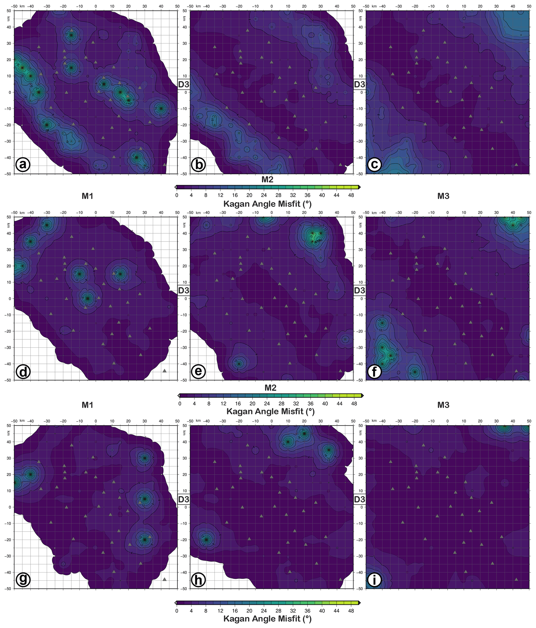
Figure 10 KAM (Kagan angle misfit) maps for retrieved focal mechanisms with D3 datasets as input data and simulating earthquakes with M1 (a, d, g), M2 (b, e, h), and M3 (c, f, i) magnitudes and FM1 (a–c), FM2 (d–f), and FM3 (g–i) theoretical fault plane solutions at 10 km depth. The level of Gaussian noise is set to 5 %.

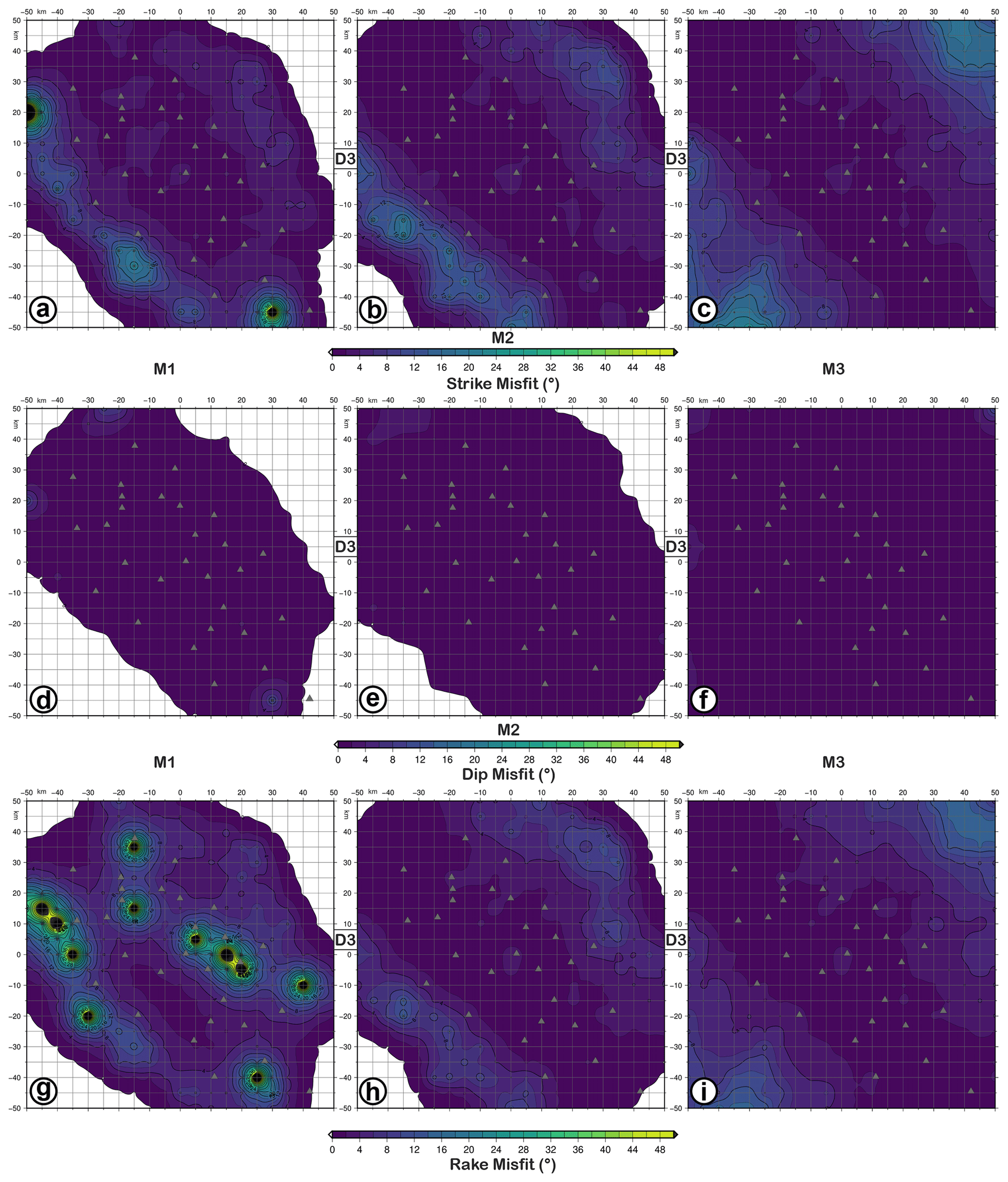
Figure 11 FMM (focal mechanism parameter misfit) maps for retrieved focal mechanisms with D3 datasets as input data and simulating earthquakes with M1 (a, d, g), M2 (b, e, h), and M3 (c, f, i) magnitudes and the FM1 theoretical fault plane solution at 5 km depth. Panels (a–c) refer to strike misfit; (d–f) refer to dip misfit; (g–i) refer to rake. The level of Gaussian noise is set to 5 %.

The accuracy of fault plane solutions evaluated using the KA misfit and D3 dataset is similar for FM1, FM2, and FM3, mostly with values lesser than 8^∘ for all the magnitudes (Fig. 10). FM2 and FM3 show a slightly higher precision than FM1 in the area inside the seismic network (see FMM, FME, KAA, and KAS maps for FM2 and FM3 in the Supplement). In the regions outside the network, where the azimuthal gap increases, the FMs better constrained in descending order are FM3, FM2, and FM1. This effect should be due to the geometric relationship between the spatial distribution of the seismic stations and the orientation of the principal axes (P, T, B) that characterize the FMs.

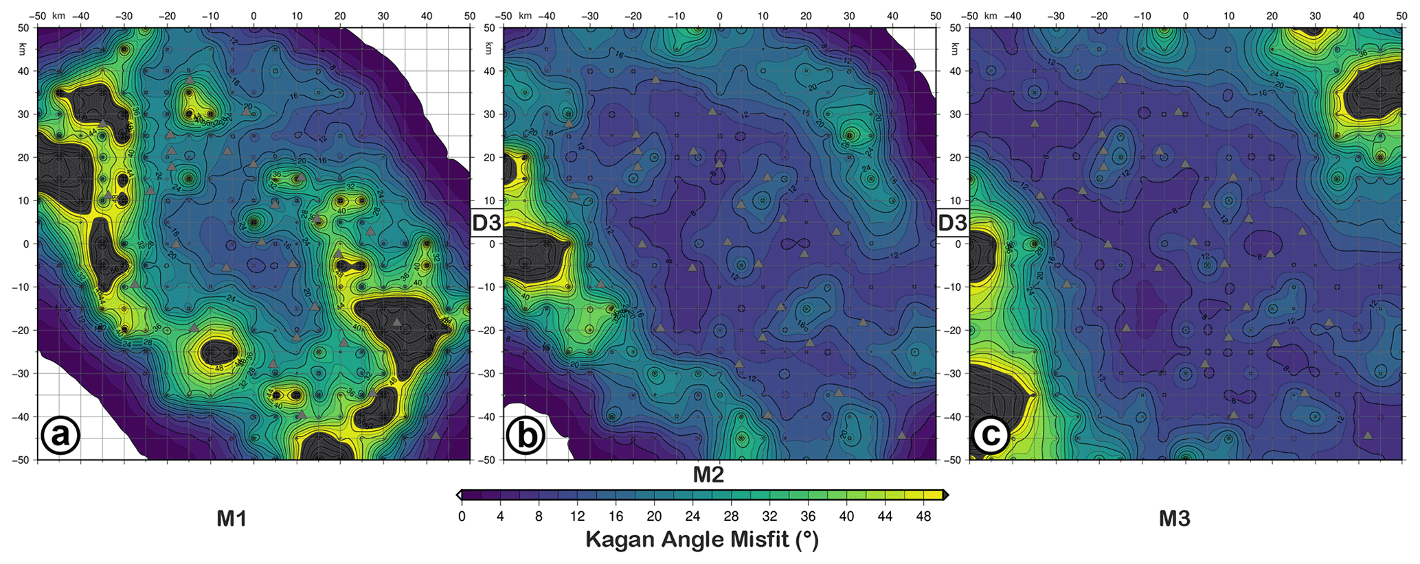
Figure 12 KAM (Kagan angle misfit) map for retrieved focal mechanisms with D3 (a–c) datasets as input data and simulating earthquakes with M1 (a), M2 (b), and M3 (c) magnitudes and the FM1 theoretical fault plane solution at 10 km depth. The level of Gaussian noise is set to 30 %.

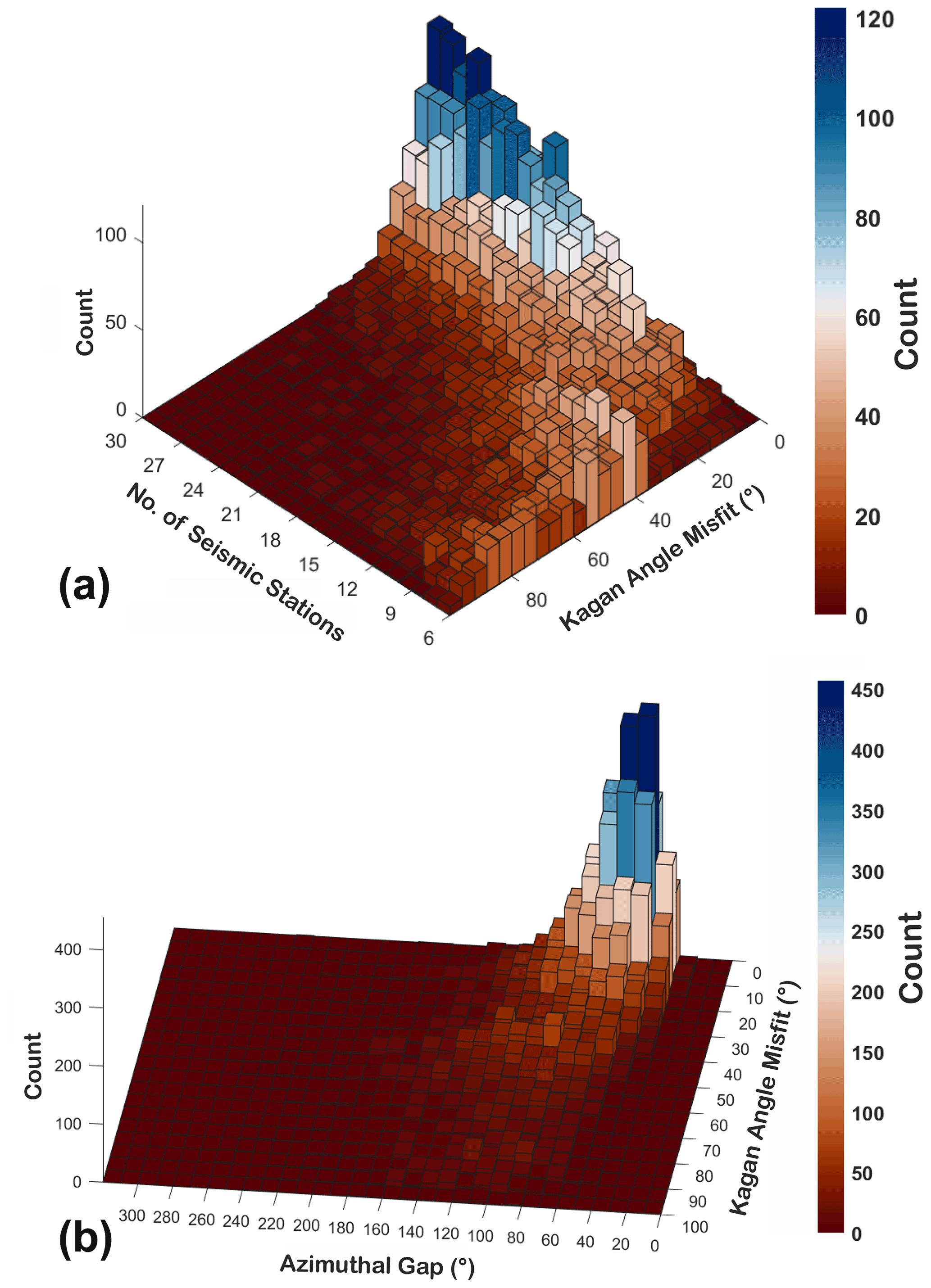
Figure 13 Three-dimensional histograms of the test results in terms of the number of stations (a), azimuthal gap (b), and KA misfit. The simulations were carried out with a free network configuration.

Considering the effect of hypocentre depth, the results achieved for earthquakes at 5 km depth, by using the D3 dataset, are overall unchanged (Fig. 11). We note that the fault plane solutions are slightly worse resolved due to a smaller number of P-wave polarities available for M2 and M3. The KA misfit is generally less than 10^∘, even though the number and the dimension of areas with $\text{misfits}>\mathrm{20}{}^{\circ }$ are greater than those obtained considering earthquakes at 10 km depth. Moreover, the dip angle shows a misfit lower than strike and rake angles for M1, M2, and M3; the accuracy of the retrieved FM parameters is mainly less than 8^∘, as shown in Fig. 11.

Previous analyses are carried out considering data affected by 5 % Gaussian error. In the last test, we simulated synthetic data adding a 30 % Gaussian error. As illustrated in Fig. 12, FM solutions show an overall larger misfit, in particular, the KA inside the seismic network is less than 20^∘. The area best resolved ($\text{KA}<\mathrm{8}{}^{\circ }$) is reduced to the central portion of the network. This result indicates that the accuracy of the spectral level ratio estimates is crucial: noisy waveforms with a low signal-to-noise ratio can critically affect the result of the focal mechanism inversion. So, seismic noise as well as the number of available stations, variable due to the operational conditions, strongly influence the capability of the seismic network to retrieve a fault plane solution. Using the results of our simulations, we classified the focal mechanism provided by De Matteis et al. (2016) according to a quality code based on the resolution of fault kinematics (Table 3). In fact, we assigned to focal mechanisms of the Irpinia instrumental seismicity qualities A, B, and C for the solutions that fall into the bins relative to FM3, FM2, and FM1 kinematics, respectively. The qualities A, B, and C correspond to the average value of the KA misfit (FM3=2.4, FM2=3.1, $\text{FM1}=\mathrm{4.5}{}^{\circ }$) calculated for M1, M2, and M3 magnitudes using D3 dataset and considering earthquakes at 10 km depth with 5 % Gaussian errors.

As a last analysis, we carried out a test in a more general framework, without a fixed network configuration. We explored the reliability of focal mechanism estimation as a function of the uniformity of the focal sphere coverage, defined by the number of recording seismic stations and the azimuthal gap. We simulated 10 400 earthquakes fixing the fault plane solution and varying (1) the number of seismic stations (6–30), (2) the take-off angle, and (3) the azimuth of each single station. For each possible number of seismic stations, we run about 400 simulations, and we randomly sampled the focal sphere varying the azimuth and take-off of the stations, thus changing the geometrical configuration of our virtual network of each simulation. We computed the KA between the theoretical and retrieved focal mechanism (best) solutions using only P polarities for each simulation. We show the results in Figs. 13 and S7 in the Supplement, as 3-D histograms and a 3-D scatter plot, respectively. In Figs. 13a, as expected, the number of stations increases, while the KA and its range of variation decrease. If the number of stations is less than nine, only few solutions have $\text{KA}<\mathrm{40}{}^{\circ }$. Figure 13b shows that most values of KA less than 30^∘ are obtained for an azimuthal gap of less than about 80^∘. In Fig. S7, the relation among the KA, azimuthal gap, and number of stations is clarified by the three-dimensional spatial point patterns as well by the projections of the data on the three coordinate planes.

6 Conclusions

We studied the focal mechanism reliability retrieved by the inversion of data recorded by ISNet, a local dense seismic network that monitors the Irpinia fault system in southern Italy. Three different datasets of seismological observables are used as input data for focal mechanism determination: (a) P-wave polarities, (b) P$/$S long-period spectral amplitude ratios, and (c) joint polarities and amplitude ratios. Starting from empirical observations, we computed synthetic data for a regular grid of epicentre locations at two depths (5 and 10 km), for an earthquake magnitude in the range 1.0–2.5, and for three focal mechanism solutions. Two different levels of Gaussian error (5 % and 30 %) are added to the data.

Our results show the following:

• The joint inversion of P-wave polarities and P$/$S spectral amplitude ratios allows retrieving accurate FM (KA misfit $<\mathrm{8}{}^{\circ }$) also for earthquakes with a magnitude ranging between 1.0 and 2.5, at depths of 5 and 10 km. Due to the low-energy magnitude, the number of P-wave polarities cannot constrain fault plane solutions.

• The spatial resolution analysis of ISNet shows that the most accurate FM solutions are obtained for earthquakes located inside the network with strike, dip, and rake misfit $<\mathrm{8}{}^{\circ }$. Nevertheless, outside the network or at its borders, acceptable solutions can be calculated even if the azimuthal coverage is inadequate (especially for M2 and M3 events). This is due to the geometrical relationship between the seismic stations and the orientation of the principal axes (P, T, B).

• The geometry of the network allows us to resolve well fault plane solutions varying between a normal and normal strike focal mechanism with strike, dip, and rake misfit generally less than 10^∘ and for the magnitude range 1.5–2.5. The network resolves a normal strike fault plane solution slightly better than a pure normal focal mechanism.

• Among the FM parameters, the dip angle shows the lowest uncertainty. Strike and rake angles have higher errors especially for M 1–1.5 earthquakes in the region outside the seismic network.

• Adding a 30 % Gaussian error worsens the accuracy of the retrieved FMs. Despite the higher uncertainty fault plane solutions (KA misfit $<\mathrm{20}{}^{\circ }$) are still resolved in the central part of the network, especially for M2 and M3.

The methodology described in this work can be a valid tool to design and test the performance of local seismic networks, aimed at monitoring natural or induced seismicity. Moreover, given a network configuration, it can be used to evaluate the reliability of FMs or to classify fault plane solutions that represent fundamental information in seismotectonic studies. Although this is a theoretical study, many earthquake scenarios with several magnitudes, locations, and noise conditions can be simulated to mimic the real seismicity.