the Creative Commons Attribution 4.0 License.
the Creative Commons Attribution 4.0 License.
 | 22 Mar 2022
Reflection imaging of complex geology in a crystalline environment using virtual-source seismology: case study from the Kylylahti polymetallic mine, Finland
Michal Chamarczuk
Michal Malinowski
Deyan Draganov
Emilia Koivisto
Suvi Heinonen
Sanna Rötsä
For the first time, we apply a full-scale 3D seismic virtual-source survey (VSS) for the purpose of near-mine mineral exploration. The data were acquired directly above the Kylylahti underground mine in Finland. Recorded ambient noise (AN) data are characterized using power spectral density (PSD) and beamforming. Data have the most energy at frequencies 25–90 Hz, and arrivals with velocities higher than 4 km s−1 have a wide range of azimuths. Based on the PSD and beamforming results, we created 10 d subset of AN recordings that were dominated by multi-azimuth high-velocity arrivals. We use an illumination diagnosis technique and location procedure to show that the AN recordings associated with high apparent velocities are related to body-wave events. Next, we produce 994 virtual-source gathers by applying seismic interferometry processing by cross-correlating AN at all receivers, resulting in full 3D VSS. We apply standard 3D time-domain reflection seismic data processing and imaging using both a selectively stacked subset and full passive data, and we validate the results against a pre-existing detailed geological information and 3D active-source survey data processed in the same way as the passive data. The resulting post-stack migrated sections show agreement of reflections between the passive and active data and indicate that VSS provides images where the active-source data are not available due to terrain restrictions. We conclude that while the all-noise approach provides some higher-quality reflections related to the inner geological contacts within the target formation and the general dipping trend of the formation, the selected subset is most efficient in resolving the base of formation.
- Article
(27259 KB) - Full-text XML
- BibTeX
- EndNote


Ambient noise (AN) seismic interferometry (SI) principles can be used to extract the reflection response of the subsurface at different scales (Daneshvar et al., 1995; Draganov et al., 2009, 2013; Ruigrok et al., 2010; Ryberg, 2011; Quiros et al., 2016). However, the original derivations of SI, as well as the majority of surface seismic applications, have considered relatively simple geological structures (sedimentary layers). It was only recently that ANSI was for the first time used for reflection imaging in much more complex crystalline rock – also known as hardrock – environments. Cheraghi et al. (2015) demonstrated that passive seismic recordings and SI are capable of providing 3D images of the moderately dipping folded volcanic rocks at the Lalor Lake mining camp in Canada. The passive results were benchmarked against an active-source 3D survey. The final conjecture of the Lalor Lake study was that future passive surveys should be acquired with longer offsets, shorter receiver spacing, and wider azimuth distribution to address the potential of the method to produce convincing images of steeply dipping reflections in crystalline rock environments.
The most recent ANSI study near Marathon, Ontario, in Canada (Dales et al., 2020) employed the abovementioned principles by combining a dense large receiver number (large-N) array with an additional receiver line that had even denser receiver spacing than the rest of the grid. In line with the already postulated selective stacking to enhance body-wave reflections (Draganov et al., 2013), the authors selectively stacked recordings (31 h out of the 30 d) along the more densely spaced receiver line. It was shown that higher-frequency (>10 Hz) body-wave sources generated by trains and cars (thus predominantly at the surface) could be used to image a major dipping layer interpreted as the gabbroic intrusion that hosts Cu–PGE mineralizations in the area, the extent of which provides crucial information for guiding mineral exploration. At the same time, the authors concluded that even better imaging could have been obtained if the active mine were closer and blasting more frequent, also providing body-wave energy from beneath the array.
The study presented in this paper was also inspired by the pioneering work at Lalor Lake. We designed a new seismic experiment in order to test the feasibility of ANSI to produce a reflection seismic 3D image of a much more complex medium when compared to the Lalor Lake mining camp setting. In 2016, we deployed a regular 3D passive seismic survey consisting of ca. 1000 receivers (details to follow in Sect. 3) recording 30 d over the polymetallic Kylylahti underground mine located in eastern Finland. The already existing detailed geological data and models as well as extensive previous and new active-source reflection seismic data acquired in parallel to the passive seismic survey made the area attractive for testing and validating the 3D virtual-source survey (VSS) methodology.
The ore-bearing ophiolite-derived altered mafic–ultramafic rocks are severely folded at Kylylahti and the main contacts are subvertical, constituting a challenge for surface seismic methods. Additionally, the rock properties are causing contacts between various rock types to be less reflective compared with, e.g., the Lalor Lake scenario. However, based on earlier active-source reflection seismic data, the main target contacts were expected to be reflective and the active mine operations were providing body-wave energy sources at depth, which is beneficial for reflection imaging in such complex medium. Initial attempts to work on the full 3D data (Chamarczuk et al., 2017, 2018) failed to provide a convincing image of the structures, and therefore our attention turned first to 2D ANSI applied along the receiver lines (Väkevä, 2019; Chamarczuk et al., 2021). Synthetic modeling results in 2D and 3D (Riedel et al., 2018; Chamarczuk et al., 2021), as well as consistent 2D images of the main structures derived along the neighboring receiver lines, allow us to extend our work to the full 3D data with more confidence. Such an approach also allowed us to test various AN preprocessing and SI techniques in a much more efficient way. Simultaneously, Chamarczuk et al. (2019, 2020) developed a methodology to automatically identify noise panels containing body-wave energy in the 3D recordings. In this paper, we further build on these earlier results and present a full-scale 3D seismic VSS approach to extract the 3D reflection response from the Kylylahti passive seismic data. To our knowledge, this is the first application of the full 3D ANSI approach to extract reflection response in a hardrock environment. However, it should be noted that despite the pioneering nature of our VSS study in the context of passive reflection imaging in hardrock environments, the first state-of-the-art applications of VSS using data from large-N arrays are related to arrays deployed in California, USA: the Long Beach array (Nakata et al., 2015) and the San Jacinto fault zone array (Ben-Zion et al., 2015).
Our paper is organized as follows. We first describe the Kylylahti 3D dataset and the associated geological background. Subsequently, we present an evaluation of the noise characteristics, including power spectral density (PSD), beamforming, and spatiotemporal techniques dedicated to quantitative body-wave content assessment. Then, by applying SI using cross-correlation, we obtain two sets of virtual-source gathers (VSGs) at each receiver location of the array, retrieved using (i) the 10 d when body-wave energy related to underground sources is stronger than the constantly present surface-wave noise and (ii) using all 30 d of data. Finally, we apply conventional reflection processing to the sets of VSGs and compare them with the active-source processing results as well as with the available detailed geological data and models in order to verify that the presented 3D VSS methodology works.
The Kylylahti polymetallic (Cu–Co–Zn–Ni–Ag–Au) semi-massive to massive sulfide ore deposit is situated in the famous Outokumpu mining district in eastern Finland (Fig. 1). Because of the long exploration and mining history of the area, a host of geological and geophysical data and models – including extensive active-source reflection seismic data that were further expanded in parallel to the passive seismic survey (Fig. 1) – are already available for assessing the results of the passive seismic survey. This is critical for validating the full-scale 3D seismic VSS approach. The Kylylahti mine was open from 2012 to 2020 and has been operated by Boliden since 2014. The Outokumpu ore belt comprises Paleoproterozoic turbiditic deep-water sediments and ophiolitic slices of upper mantle rocks from oceanic lithosphere forming the Outokumpu nappe thrusted onto the Archaean basement and subsequently strongly deformed. Metamorphic alteration changed the originally depleted upper mantle rocks into Outokumpu assemblage serpentinite–skarn–carbonate–quartz rocks hosting the mineralizations (Peltonen et al., 2008). In the Kylylahti area, the following four main units can be distinguished (Peltonen et al., 2008) (Fig. 1): (1) the Kylylahti semi-massive to massive sulfide (S/MS) mineralization hosted in (2) Outokumpu ultramafics (OUMs) that mainly consist of serpentinite and talc–carbonate rocks with (3) fringed alteration zones composed of carbonate–skarn–quartz rocks, the altered Outokumpu ultramafics (OMEs). In combination, the nearly N–S-trending and nearly vertical OUM and OME units are called the Outokumpu assemblage rocks (referred to as the Kylylahti formation).
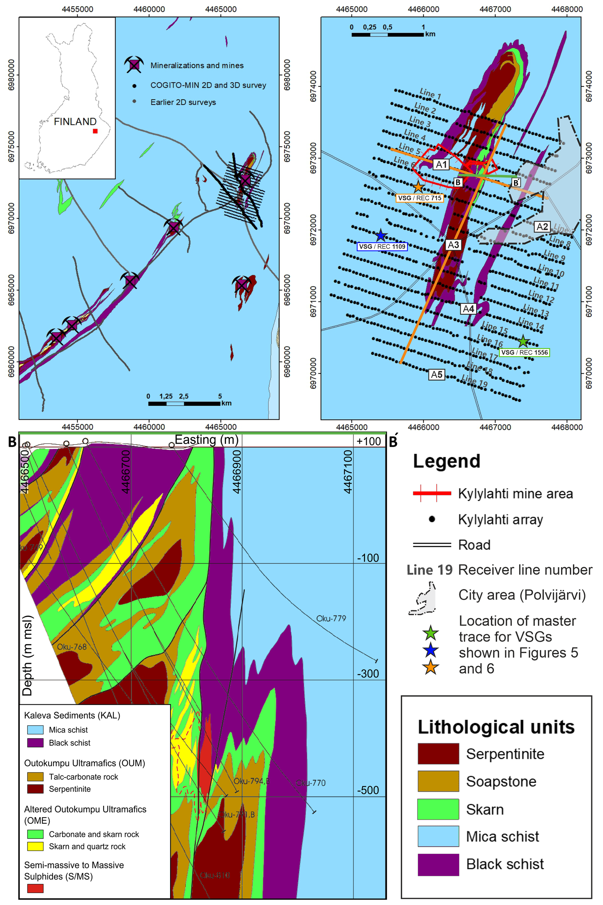
Figure 1Location of the Kylylahti mine and Kylylahti array in the Outokumpu belt (top left panel). Location of the 3D passive seismic survey (top right panel). B–B′ is a cross-section through the Kylylahti deposit (bottom left panel; modified after Peltonen et al., 2008, and Riedel et al., 2018). Orange lines mark a representative crossline and inline location of the 3D passive seismic volume. A1–A5 denote five representative areas of ambient noise in the Kylylahti area that are used to compute power spectral density (PSD) in Fig. 3a: the mine (A1), a city (A2), a roundabout (A3), a road (A4), and a quiet area (A5).
In the Kylylahti area, the Outokumpu assemblage rocks are in nearly vertical contact with the (4) regional Kaleva Sedimentary Belt (KAL), consisting of mica schist and black schist. Black schists often interweave with the Outokumpu assemblage package, with various rock contacts repeated several times. Because of the complex geometry (see cross-section in Fig. 1), the Kylylahti formation remains a difficult target for surface seismic methods. Besides the obvious strong impedance contrast between the S/MS mineralizations and the host rocks, rock-property measurements (Luhta, 2019) indicate sufficiently strong contrasts in acoustic impedances, in the Kylylahti area mainly arising from contrasts in densities, to produce a detectable reflection at the contact of the OUM/OME rocks and the interlayered and surrounding schists. Some reflectivity is also expected to arise from the lithological changes within the Outokumpu assemblage, especially due to the alterations (e.g., the talc–carbonate rocks exhibit a significantly lower P-wave velocity than the serpentinites).
Based on the rich borehole data (>1300 boreholes) a detailed geological model was created for the 3D volume covered by the boreholes by the mine operator (Boliden) and used to create a seismogeological model by Riedel et al. (2018). The geological model was averaged into the above-described four main units and populated with the average P-wave velocities and densities from laboratory measurements on core samples. This model was used, e.g., by Chamarczuk et al. (2021) to assess the results of the 2D ANSI based on synthetic and field data, and it is used in this paper to validate the results and to support the interpretation. However, it should be noted that the geological model provides a reliable account of the geology only within the extent of the borehole data, as further discussed when describing the interpretation of the passive images presented in this paper.
The passive seismic experiment was performed in the Kylylahti mine area between early August and late September 2016 as a part of the COGITO-MIN (COst-effective Geophysical Imaging Techniques for supporting Ongoing MINeral exploration in Europe; Koivisto et al., 2018) project. This project aimed for development of an efficient integrated exploration workflow ranging from regional-scale exploration to detailed resource delineation and mine planning including an active-source and passive seismic component. We used 994 vertical-component receiver stations distributed regularly over the 3.5×3 km area with a 200 m line spacing and 50 m receiver interval (Fig. 1). Surface conditions varied between exposed bedrock and swamps.
Each receiver station consists of a Geospace GSR recorder and six 10 Hz geophones, bunched together and buried whenever possible, recording at a 2 ms sample rate 20 h d−1 for 30 d. As a result, we recorded over 600 h of ambient noise data per receiver. In addition, the 3D grid recorded irregularly distributed active shots (both explosives and vibroseis) specifically designed for the 3D active survey (Singh et al., 2019) as well as active shots used for the 2D seismic profiles crossing the 3D grid (Heinonen et al., 2019). Therefore, a low-fold 3D active-source seismic survey was also acquired to benchmark the results of the passive survey. The active-source data (30 s long windows including the active shots) were removed from the passive data before the analyses presented in this paper. The survey area is located in the direct vicinity of the town of Polvijärvi (Fig. 1). Two fairly busy state roads cut through the survey area. A roundabout connecting both roads is located in the center of the array. The Kylylahti mine is located to the northwest from the roundabout. The access to the mine is along gravel roads, used extensively by hauling trucks. The Kylylahti mine was active during the whole recording period. Routine mining activities included drilling (surface and underground), transporting ore and waste rock (surface and underground), scaling (underground), and mine ventilation (surface) among others. A source of strong energy is provided by mine blasts, which occurred daily at depths ranging from 100 m down to approximately 800 m below the surface.
As advocated, e.g., by Draganov et al. (2013), for reflection retrieval from ANSI, a form of selective stacking is typically required. Towards this end, Chamarczuk et al. (2019) developed a two-step wave-field evaluation and event detection method (TWEED) to be able to identify noise panels containing body-wave energy. This method was later augmented by a machine-learning approach to automatically classify (cluster) different noise sources present in the continuous recordings (Chamarczuk et al., 2020). TWEED was used to identify noise sources that were subsequently used for 2D ANSI imaging comparing the all-noise approach (i.e., stacking all the data) vs. the selective stacking approach using subsets of the evaluated noise panels (Chamarczuk et al., 2021). At the same time, various AN preprocessing and SI techniques (e.g., cross-correlation vs. multidimensional deconvolution) were tested at the selected receiver lines from the full array. Overall, the methodology adopted in this study builds on these earlier results and can be summarized as follows: (1) general description of the recorded wave field to identify dominant frequencies, directions of illumination, and apparent velocities of the AN sources; (2) quantification of body-wave energy present in the recorded data using the TWEED approach and obtaining spatial distribution of the noise sources; (3) actual SI data retrieval, i.e., obtaining VSGs through cross-correlation for the two sets of data (i) for 10 d when the body-wave events are dominating and (ii) for the full 30 d of data; (4) standard hardrock reflection seismic processing of the obtained VSGs. The above four processing steps, together with validation and interpretation of passive results using a direct comparison to an active survey as a benchmark and to the available detailed geological data and models as a reference, add up to the five main processing blocks forming the full-scale 3D seismic VSS methodology for the purpose of near-mine mineral exploration developed in this study (see flowchart in Fig. 2, where the gray-gradient-colored blocks in the right column indicate our modifications of the state-of-the-art AN imaging workflow proposed by Draganov et al., 2013).
4.1 General ambient noise characteristics
The main prerequisite for the reflection imaging based on ANSI is the body-wave content in the recorded wave field (Draganov et al., 2013). We assess the body-wave content in AN recordings from Kylylahti in three steps: first, we determine the temporal and spatial variations of AN frequency–amplitude characteristics using power spectral density (PSD). Then, we characterize the dominant frequencies and velocities of the recorded AN with beamforming, and finally we directly assess the body-wave events with a dedicated detection and location procedure that provides an objective, quantitative measure of the recorded body-wave energy.
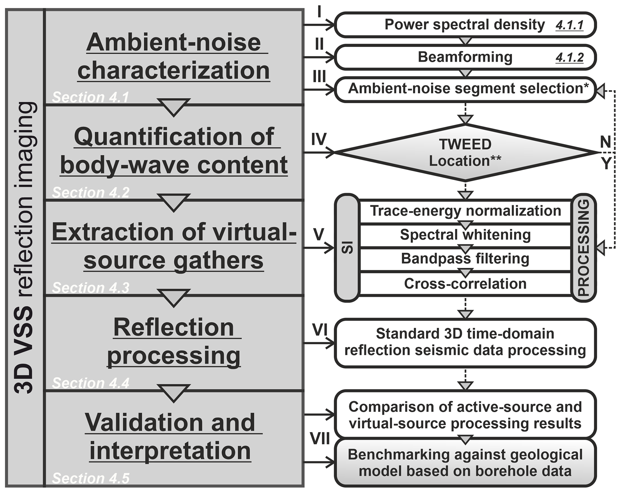
Figure 2Summary of the 3D virtual-source survey methodology for the purpose of near-mine mineral exploration. The left column presents the core of the flowchart: it contains five main processing blocks representing Sect. 4.1–4.5. The detailed processing steps performed within each main processing block are shown in the right column. The sequence of processing is indicated by roman numerals. Gray-gradient-colored blocks in the right column indicate our modifications of the state-of-the-art ambient noise imaging workflow proposed by Draganov et al. (2013). The single star symbol denotes the user-dependent “ambient noise segment selection” processing step, in which the initial selection is based on the beamforming results and later verified by TWEED. The double star symbol denotes the location procedure, which supports the TWEED verification but is not mandatory.
4.1.1 Power spectral density
We use PSD plots to assess the temporal and spatial distribution of frequency–amplitude features of the seismic noise in the Kylylahti area. To simplify the description of AN in the Kylylahti area, we analyze five representative areas (denoted with the letter “A” in Fig. 1) that allow clearly emphasizing the differences in frequency–amplitude content of the data recorded in different parts of the array. These are the mine (A1) (A2), a roundabout (A3), a road (A4), and a quiet area (A5). For each area, we take data from five adjacent stations from the Kylylahti array, split their continuous noise records into 0.5 h long windows with 50 % overlap, compute the PSD, and average the PSD values over these five stations (Fig. 3).
The frequency spectra related to the mine (A1 in Fig. 3a) exhibit the broadest frequency range out of all areas, with the most energetic part between 25 and 90 Hz. With increasing distance from the mine, we observe diminishing energies related to the higher frequencies, as well as strengthening of the contribution from energies in the lower-frequency range (10–30 Hz) associated with the road traffic and other surface sources. This is clearly visible for the city area (A2) and roundabout (A3) PSD spectra, which still contain the energies up to 90 Hz due to their proximity to the mine. The exact contribution from road traffic to the AN recordings from Kylylahti is observed in the PSD plot for stations in areas that are located in the direct vicinity of the road (A4 and A5). The frequency spectra related to the road traffic exhibit the most energetic parts up to 30–35 Hz, with a peak at around 20–30 Hz, which is also characteristic for the surface waves observed, e.g., in 2D active-source data (Heinonen et al., 2019).
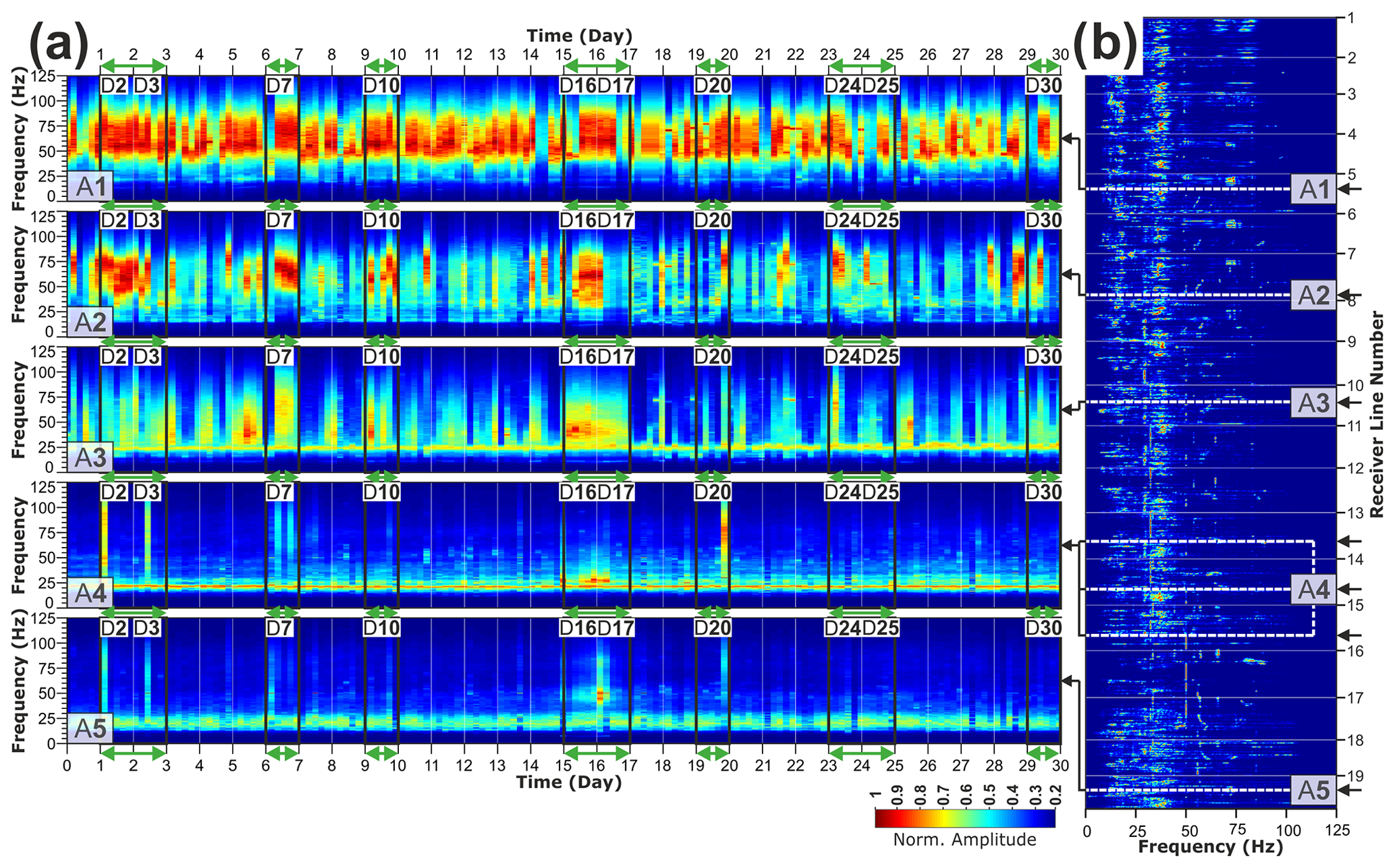
Figure 3Temporal (a) and spatial (b) variation of noise spectrograms. (a) Each panel represents power spectral densities (PSDs) computed for each day of recording using receiver stations located in the representative areas highlighted in Fig. 1. Days highlighted with green arrows correspond to beamforming panels highlighted with green circles in Fig. 4a. (b) PSD for a single day of recording using every receiver station of the Kylylahti array. White dashed lines highlight receiver stations corresponding to the representative areas shown in (a). Amplitudes are independently normalized in each panel. Two regimes of high power density are observed at frequency ranges of 10–30 and 40–90 Hz.
It can be concluded that the main source of higher frequencies (25–90 Hz) in the recording area is the mine and that the higher-frequency part of AN generated in this area is still recorded even in the far end of the Kylylahti array (note that the energies associated with the frequency range 40–90 Hz are still visible in PSDs for receiver lines 15–19 in Fig. 3b). However, due to the remoteness of areas A4 and A5 (see Fig. 1), the PSD computed for receiver lines located in these regions exhibits lower amplitudes in the frequency range 40–90 Hz compared to road-traffic-induced energies (10–30 Hz). This is further confirmed by PSD computed for the whole array (Fig. 3b); the transition from higher to lower frequencies is observed for subsequent receiver lines. Due to the difference between PSD spectra associated with the road traffic and mine area, we identify the higher frequencies generated in the mine area as potentially associated with body-wave sources required for SI reflection imaging.
4.1.2 Beamforming
After the PSD analysis, we use beamforming to assess how much and which parts of the data are dominated by body-wave events such that, when stacked, they would allow obtaining the omnidirectional coverage of the stationary-phase regions (Snieder, 2004). In Fig. 4a we show the results of standard beamforming (Rost and Thomas, 2002) analyses calculated and summed over 20 h recorded during each single day in the frequency range between 3 and 5 Hz. Note that to avoid aliasing the theoretical limit on beamforming is imposed by the Nyquist wavenumber (Rost and Thomas, 2002), which in the case of receiver line spacing of 200 m and velocity of 2 km s−1 gives Hz. These daily beamforming plots represent partial contributions to the stacked beamformer output in Fig. 4b, which is the summed output of all 30 daily results. The maximum values shown in Fig. 4b represent the dominant AN contributions that were persistent during most of the recording time and which can be identified in the daily beamforming plots (compare individual panels in Fig. 4a). The recorded wave field is coming from the NNW, a narrow area in the E, and a broad range of azimuths in the SE. These directions are consistent with the general orientation of areas indicated in the PSD plots and associated with noise sources located at the mine site (A1), the town of Polvijärvi (A2), and the roads (A3, A4, and A5). We can distinguish three groups of arrivals based on the apparent velocities (Fig. 4b): (1) V=1–3 km s−1 likely representing surface waves (associated with S, and SE areas), (2) V=3–4 km s−1 likely associated with S-wave arrivals (mostly SE direction), and (3) V>4.8 km s−1 interpreted as P-waves coming from the NNW and S directions. The red–green circle in the summed beamforming output (Fig. 4b) denotes the data-driven separation between the P-waves and surface waves in the Kylylahti area (note here a wide range of azimuths associated with beamforming values above 4 km s−1 in Fig. 4b). The same line is projected on the results computed for each day. We use this line to distinguish between the daily beamforming results that are dominated by P-wave arrivals (see green circles in Fig. 4a) and those with more notable surface-wave content (see red circles in Fig. 4a). It is important to note here that while the number of highlighted days dominated by body-wave arrivals (10) is smaller than those dominated by surface-wave sources, the body-wave arrivals were present during most of the recording days. As shown by Draganov et al. (2013), Roots et al. (2017), and Dales et al. (2020), selecting only data periods when noise is dominated by sources in the stationary-phase region for reflection retrieval may provide results with higher quality than stacking all noise. On the other hand, stacking all noise represents an attempt to utilize the full capacity of ANSI by incorporating all body-wave events which occurred during recording time but were not dominant during the days designated as dominated by surface-wave noise. To address these two fundamental views on SI processing, we create two subsets of AN recordings: for 10 and 30 d, with the former representing selectively stacked periods of AN dominated by arrivals with high apparent velocity (these days are highlighted with green circles in Fig. 4a) interpreted to represent body-wave events, and the latter allows testing the full capacity of recorded data (see Sect. 5.5 for a more detailed discussion of both subsets). The subset of 10 d used for evaluation of the selective stacking approach in this study consists of the following days denoted in Fig. 4a: D2, D3, D7, D10, D16, D17, D20, D24, D25, and D30.
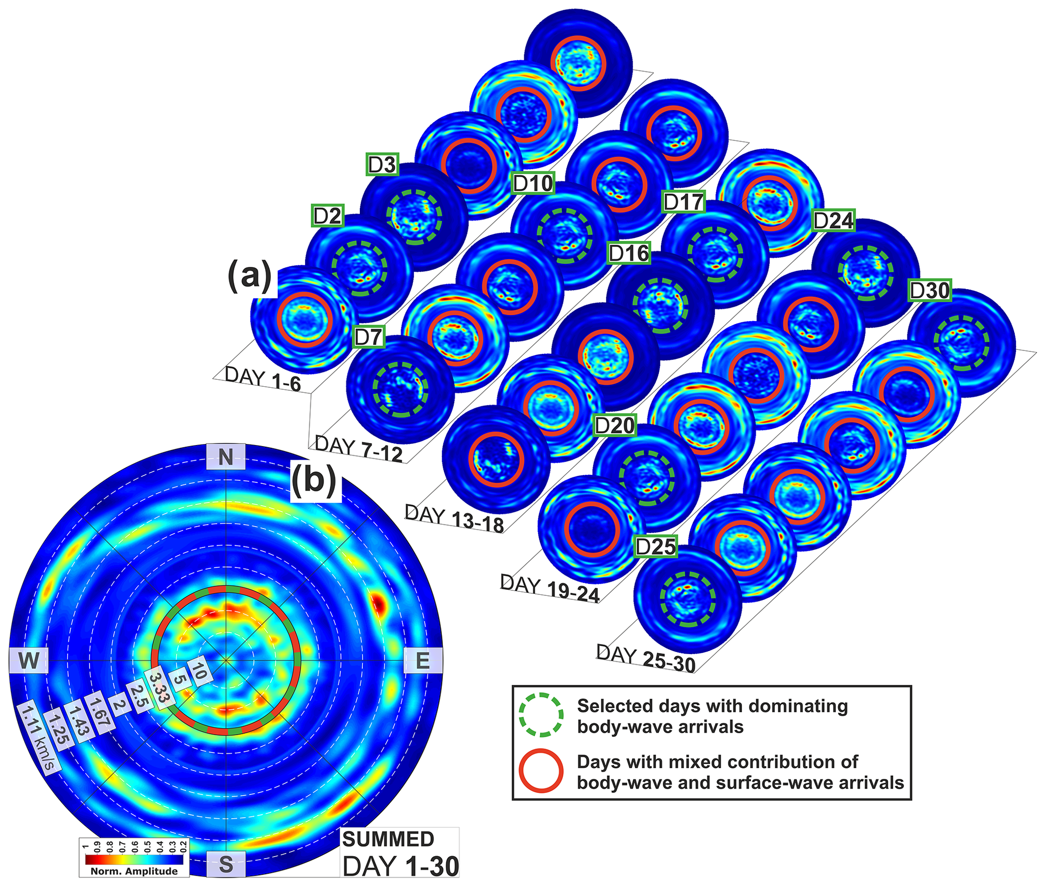
Figure 4Directional beamforming analysis of recorded ambient noise (AN) using all available Kylylahti recordings. (a) Beamforming outputs calculated for 20 hourly panels from 30 d of recording time. Each panel in (a) represents analysis for 1 d of recording. Panels are displayed in chronological order. (b) Summed output of the results shown in (a). Maximum values from each hourly (a) and daily (b) result are displayed as a function of apparent velocity and azimuth for the frequency range 3–5 Hz. The north direction (N) has an azimuth of 0∘. The azimuth increases to the west (i.e., counterclockwise), and apparent velocities increase toward the center of the circles. Warmer colors indicate directions of strong incoming energy. Green dashed circles in (a) highlight 10 daily AN recordings dominated by arrivals with apparent velocities >4.8 km s−1 and used for initial selection of the 10 d subset as the representation of the selective stacking approach in this study. In Sect. 4.2, this initial subset of data denoted with green circles in (a) is evaluated by TWEED to confirm that the AN recordings associated with apparent velocities >4.8 km s−1 are related to body-wave events and eventually used to obtain the selectively stacked virtual-source gathers shown in Figs. 6 and 7 described in Sect. 4.3. The same days are highlighted with green arrows in Fig. 3a.
4.2 Quantification of the body-wave content
After the qualitative assessment of the AN sources in the Kylylahti area, the next step is to confirm that the AN recordings associated with high apparent velocities (V>4.8 km s−1), identified using beamforming, are related to actual body-wave events. As opposed to PSD and beamforming analyses, the quantification of the body-wave content is performed over short time windows (10 s long) and utilizes the aforementioned TWEED method for detection of body-wave content and InterLoc (Dales et al., 2017) for computing the locations of the detected sources.
The essence of TWEED (Chamarczuk et al., 2019) is that it allows the detection of body-wave arrivals by scanning the neighboring receiver lines from the regular 3D array. It ensures that the surface waves arriving off the line and having apparent velocities similar to body waves are discarded. InterLoc is similar to beamforming, but instead of scanning azimuth and velocities, it scans the different location points and the input comprises cross-correlated waveforms instead of the noise panels. It is based on computation of the model-based time lags at each scanned point of a model grid. The Kylylahti formation (see description of the Outokumpu assemblage rocks in Sect. 2) can be considered the “inclusion” in the simple, single-layer background (see description of the KAL unit in Sect. 2) and does not affect the global average velocity. Therefore, in this study we use a constant-velocity model of 5 km s−1 as an approximation of the crystalline rock environment in the Kylylahti area. We estimate the maximum possible error from the constant-velocity model selection as 10 %. The computed time lags are used to time-shift the cross-correlation between the every receiver pair and sum the cross-correlation functions per each node of the grid. The source is found at the grid node in which the sum of the time-shifted cross-correlation functions yields the highest value.
In Fig. 5a we show an example of a noise panel containing a clear body-wave event detected using TWEED and recorded by every receiver line of the Kylylahti array. In Fig. 5b and c we show the InterLoc result in the horizontal and vertical plane for the body-wave event shown in Fig. 5a. With respect to the limited capacity of the surface array for source depth estimation, to evaluate the approximate depth of sources, we computed InterLoc results assuming grid points spaced at 10 m between depths of 100 and 800 m. In Fig. 5c, we show the exemplary results (using the event from Fig. 5a) obtained for every fifth scanned depth. The slice with the clearest focus and highest amplitude is chosen as the most probable source depth (indicated with black arrows in Fig. 5c). In Fig. 5d and e, we show the final result of the joint TWEED and InterLoc approach applied to the total volume of Kylylahti data showing the 3D locations of all 1093 detected body-wave events (the green dot denotes the location of the exemplary event shown in Fig. 5a), which are clustered along a conical area directly beneath the array (see Chamarczuk et al., 2019, for more detailed interpretation of the detected events). The depth range (−800 to ∼100 m) agrees with the known extent of the Kylylahti mining activities. The color of the dots in Fig. 5d and e represents the separation between body-wave events that were detected inside the subset of 10 d dominated by the body-wave events (310 events marked with black dots), as indicated by the beamforming (see green circles in Fig. 4a) and PSD (see green arrows in Fig. 3a), and the body-wave events detected during the remaining 20 d (783 events marked with red dots).

Figure 5Performance of the combined TWEED and InterLoc processing scheme. (a) Scheduled mine event (underground blast) detected with TWEED, representing the typical body-wave event recorded by the Kylylahti array. Horizontal black lines mark the spatial extent of 19 receiver lines forming the complete Kylylahti array. (b) InterLoc output computed for the body-wave event shown in (a) using a 10 s recording detected with TWEED. The color scale represents the normalized amplitude of the InterLoc output. Black triangles indicate geophone locations, and the red polygon corresponds to the mine location. (c) InterLoc output for a set of discrete depth intervals. Each result in (c) was normalized using the global maximum from all evaluated depth intervals. The x−y section at −450 m of depth exhibiting the clearest focus and highest amplitudes is highlighted with black arrows and represents the most probable depth of the event shown in (a). (d) x−y and (e) 3D spatial distribution of the collection of sources at depth estimated during the 30 recording days projected on a map with the Kylylahti array (black triangles) and geographical coordinates. Dots represent the locations of the maximum InterLoc values of each detected body-wave event. The location of the event shown in (b) is denoted with a green circle. Black dots indicate the location of events, which were detected inside the subset of 10 d, highlighted in Figs. 3 and 4 and used to evaluate the SI selective stacking performance. Red dots show the locations of events from the remaining 20 d.
Essentially, the quantification of the body-wave content shows that the passive data include a significant number of body-wave events originating from subsurface sources. This verifies that the high-velocity arrivals observed in the beamforming analysis are actually related to body-wave events and not to some inline surface-wave sources. In proportion, the number of body-wave events is not any higher during the 10 d dominated by the body waves than during the rest of the 30 d of overall recording time. However, since these 10 d are characterized by noticeably lower low-velocity surface-wave activity, they are dominated by the high-velocity body waves.
4.3 Extraction of virtual-source gathers
In this subsection, we retrieve two sets of VSGs for reflection imaging: using AN recordings from the 10 d dominated by the body-wave events, during which events highlighted with black dots in Fig. 5d and e occurred, and using all data (30 d). The processing described in this subsection is the same for both sets of data with the only difference being the number of daily recordings used as an input. As evidenced by the daily PSD temporal variations (Fig. 3a) and the daily beamforming results (Fig. 4a), high-frequency and high-apparent-velocity arrivals occurred during most of the recording time (primarily associated with the mine activity). Therefore, the actual number of body-wave events recorded by the Kylylahti array is likely higher than the number of events that were detected with TWEED. To incorporate the possibly omitted body-wave arrivals, we decided to use entire daily recordings rather than only selected 10 s time windows with the detected events.
To retrieve VSGs, we divide the daily AN recordings into 30 min noise panels. Prior to cross-correlation, all traces of each panel are normalized by applying a trace-to-trace amplitude balancing (trace energy normalization; Draganov et al., 2013) to ensure that energy from all subsurface sources is equally weighted. Next, each noise panel is subjected to spectral whitening such that the energy of all traces in a noise panel is brought to the same level of amplitudes in the frequency domain. The spectral whitening removes any contributions related to noise-source wavelets and removes the necessity for wavelet deconvolution. The spectral whitening guarantees that the amplitudes of the different frequencies in the band of interest are equalized, while energy normalization guarantees equalization of the amplitudes among traces and among noise panels. Finally, we apply bandpass filtering (25–35–90–120 Hz) to reject parts of the spectrum associated with surface waves. This simple preprocessing sequence is known to be an effective solution in ANSI-based reflection imaging studies (see, e.g., Quiros et al., 2016).
For each 30 min noise panel, the cross-correlation is calculated between specific receiver positions acting as a master trace (i.e., reference receiver) and every other receiver position from the Kylylahti array (i.e., with the remaining 993 receivers, which gives 987 042 calculations per noise panel and a total of 118 445 million calculations for all 1200 noise panels). Cross-correlating a master trace with every other receiver from the array using a single noise panel yields VSG as if the shot was acquired at this master trace location. This procedure is performed for each noise panel, and after processing all 1200 panels the procedure is repeated for the next master trace until all 994 receivers are used as a master trace. Consequently, we obtain 1200 VSGs for each receiver position. The final step is stacking VSGs from all panels per each receiver location. Hence, we end up with the collection of 994 VSGs representing the full-scale 3D VSS as if the shots were acquired one by one at every receiver position of the Kylylahti array.
We assess the quality of the retrieved VSGs by checking the feasibility of the virtual-source data to retrieve the same reflection arrivals that are present in the active-source data. Note, though, that the complexity of the medium, as well as the relatively large receiver intervals (50 m), makes it very difficult to follow reflections in the shot gathers even in the case of active data (Singh et al., 2019). Despite that, reflections were identified in the co-located datasets. Figures 6 and 7 show a comparison of the selected active-source shot gathers with the co-located VSGs. For each shot, we show six receiver lines to ensure that the retrieved reflections exhibit a truly 3D nature (we expect to observe the same event on adjacent receiver lines). The VSGs were obtained by cross-correlating master trace receivers 715 (Fig. 6a), 1109 (Fig. 6b), and 1556 (Fig. 7), which are located along receiver lines 7, 11, and 15, respectively (see receivers marked with stars in Fig. 1), with every other receiver of the Kylylahti array. The arrows indicate parts of the data associated with the same reflection arrivals, as identified in the active-source gathers. Both the signal-to-noise ratio (SNR) and the move-outs of the reflection arrivals slightly vary between passive and active data. Furthermore, at larger offsets (off-end receiver lines), the presence of artifacts in the passive data does not allow for the recovery of reflection arrivals (see black arrows in Figs. 6 and 7 indicating the artifacts).
Inspecting the reflection recordings from the co-located passive and active-source data confirms that passive data allow retrieving the reflection response of the medium, albeit in some places obscured by artifacts. Similarly to active-source data, we expect this reflection response to be further enhanced by stacking and migration (Singh et al., 2019). Note that receivers 715, 1109, and 1556 (Fig. 1) were selected such that each of them is located in proximity to a different dominant noise contributor: the mine (A1), a roundabout (A3), and a road (A4), respectively (see Sect. 5.2 where we explain the link between AN characteristics and the VSG quality).
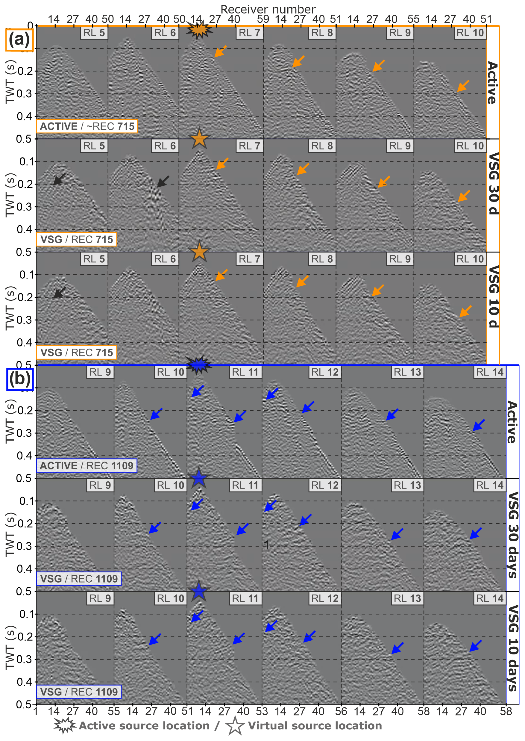
Figure 6Comparison of exemplary co-located 3D common-source gathers using active and passive data. The active-shot gathers are filtered using a bandpass filter (25–35–90–120 Hz) to have the frequency content of the passive data. For each gather, we show six receiver lines (RLs). (a) Common-source gathers co-located with receiver station 715: (top row) active-shot gather, (middle row) VSGs obtained using 30 d of noise, and (bottom row) VSGs obtained using 10 d of noise. (b) Common source gathers co-located with receiver station 1109: (top row) active-shot gather, (middle row) VSGs obtained using 30 d of noise, and (bottom row) VSGs obtained using 10 d of noise. (a) The orange and (b) blue arrows on both active and passive data highlight the position of reflection arrivals observed in active-source data and projected on co-located VSGs. Black arrows indicate artifacts characteristic for passive data. TWT stands for two-way travel time.
4.4 Reflection processing
The reflection processing workflow for the virtual-source data was modified from the one derived for processing the active-source survey data (Singh et al., 2019). Despite the fact that the active survey and VSS differ in the crossline source spacing (20–100 m vs. 200 m), we used the same size of the CDP bins (25×25 m) and the same binning grid. In the case of the passive data, this leads to some empty crosslines. Considering different shot geometries and number of shots (736 active vs. 994 virtual shots), the stacking fold is higher for the passive data (max. 700) compared with the active data (max. 160). Below is the list of the most important processing steps.
-
Read VSGs
-
Geometry setup (25×25 m bins)
-
Refraction statics (from active data)
-
AGC (500 ms)
-
Predictive deconvolution ( ms)
-
Bandpass filter (20–25–100–120 Hz)
-
Mild F-X deconvolution
-
Top mute
-
Sort to CDP
-
NMO correction (velocities from active data)
-
Post-NMO mute
-
Stack with SQRT-fold normalization
-
Constant-velocity 2.5D Stolt migration (inlines first, then crosslines)
-
Mild F-X deconvolution in the crossline direction (as interpolator of missing bins)
-
Whole-trace equalization
4.5 Validation and interpretation
Here, we compare the 3D active-source and virtual-source processing results. In both cases, we show post-stack migrated data. The comparison is facilitated by the use of the same binning grid. Empty crosslines in the passive data were interpolated using mild F-X deconvolution. On top of the migrated stacks, we also display the geological model based on extensive borehole data described in Sect. 2. This helps us to determine the location of the expected most prominent reflectivity contacts (mineralization vs. OUM/OME and the contacts between OUM/OME and KAL). We first analyze inline 1040 (see Fig. 1 for location) and then several corresponding crosslines, for which the reflectivity between the passive and active data is most consistent.
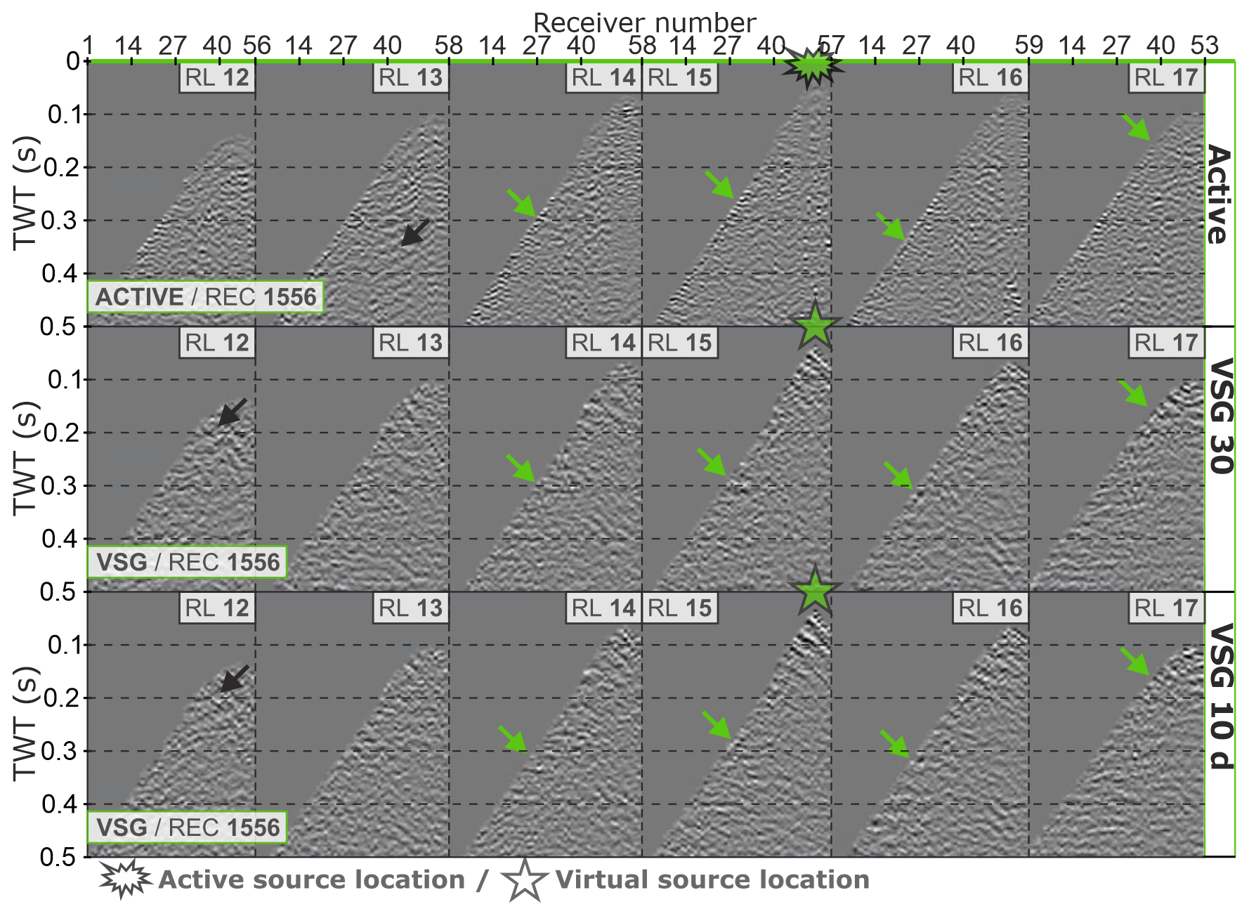
Figure 7Comparison of exemplary co-located 3D common-source gathers using active and passive data. The active-shot gathers are filtered using a bandpass filter (25–35–90–120 Hz) to have the frequency content of the passive data. For each gather, we show six receiver lines (RLs). Common-source gathers co-located with receiver station 1556: (top row) active-shot gather, (middle row) VSGs obtained using 30 d of noise, and (bottom row) VSGs obtained using 10 d of noise. The green arrows on both active and passive data highlight the position of reflection arrivals observed in active-source data and projected on co-located VSGs. Black arrows indicate artifacts characteristic for passive data. TWT stands for two-way travel time.
A comparison of the 3D-processed images along inline 1040 of both surveys is shown in Fig. 8a–c and g. Red arrows indicate positions of reflections associated with some main lithological contacts within the ore-bearing Kylylahti formation, as identified in the active data and verified by the geological model (see events marked with arrows 1–3 in Fig. 8c). The area marked by the blue rectangle in Fig. 8a–c and g denotes a gap in fold due to the active-shot distribution. In this case, the passive data supplement the image obtained from the active data by providing reflectivity in places where inline 1040 from the active survey has no data (see, e.g., the orange dashed line in Fig. 8b and c indicating how the continuity of a single reflection event can be obtained by joint analysis of active and passive data).
In the middle row of Fig. 8, we show crossline 1068 of the active survey (Fig. 8d) and passive surveys obtained using 10 d (Fig. 8f) and 30 d (Fig. 8e). In this case, the result from 10 d of AN contains mildly dipping, continuous reflection that is associated with an internal contact between an OUM/OME unit and black schists of KAL (see event marked with arrow 6 in Fig. 8f). Note that the extent of the KAL unit surrounding the OUM/OME unit in Figs. 8 and 9 is no longer constrained with the borehole data, and a series of repetitions of the OUM/OME units and black schist interlayers is expected before hitting the actual base of the Kylylahti formation and the surrounding mica schists. Interestingly, the same feature is also imaged in the result from 30 d of AN (Fig. 8e); however, it is characterized by a lower SNR and a different spatial extent when compared to the results from 10 d (compare the event marked with arrows 7–8 in Fig. 8e with the event marked with arrow 6 in Fig. 8f). Comparing the passive results from crossline 1068 obtained from 10 (Fig. 8f) and 30 d (Fig. 8e), we conclude that the all-noise approach provides higher-quality reflections related to the mineralization (see event marked with arrow 5 in Fig. 8e) and the general dipping trend of the Kylylahti formation (note the deep reflector marked with arrows 7–8 and the overall dip of the reflections in Fig. 8e), while the 10 d stack is most efficient in resolving the continuous reflector segment confirmed by the geological model to represent a contact between the OUM/OME unit and black schists (KAL) (see arrow 6 in Fig. 8f). This shows that the missed events in the subset of 10 d are useful and both approaches are valuable in a complementary fashion (as shown in Draganov et al., 2013).
For the above reasons, to showcase the consistency of imaging with passive survey, we focus on the clear reflection events associated with the contact between the OUM/OME unit and black schists (KAL) at the edge of the extent of the borehole data used to constrain the geological model shown in Figs. 8 and 9 and analyze results from 10 d of AN using three consecutive crosslines (1082, 1084, 1086; shown in Fig. 9a–c, respectively) that pass through the area of inline 1040, where the passive reflections from the right part of the bottom (arrows 1–3 in Fig. 8c) and the top (arrow 4 in Fig. 8c) of the OUM/OME unit shown in Figs. 8 and 9 were highlighted. On these crosslines, we consistently observe a weak dipping event (denoted with red arrows in Fig. 9a–c), which seems to correspond to the extent of the shown OUM/OME unit (constrained by the extent of the borehole data; see Fig. 9d–f where the geological model is overlaid on the same crosslines as in Fig. 9a–c). Specifically, we highlight here crossline 1084 (Fig. 9e), where arrows 9–10 mark the continuous, dipping reflection event corresponding to the extent of the shown OUM/OME unit, and arrow 11 is pointing to the prolongation of the same event that extends beyond the known extent of the shown geological model based on the borehole data (i.e., the bottom of the geological model).
The Kylylahti active-source 2D and 3D data (Heinonen et al., 2019; Singh et al., 2019) were used together with the available borehole data to interpret the base of the Kylylahti formation (purple surface in Fig. 10). In the active-source data, the Kylylahti formation is characterized by piecewise reflectivity, the extent of which outlines the overall formation. Because of the dominating nearly vertical orientation of the lithological contacts within the Kylylahti formation, the reflective segments are typically fairly short. In the active-source 3D data, the base of the overall Kylylahti formation, embedded in the surrounding mica schists, is also only occasionally associated with more continuous reflective segments (Singh et al., 2019). In Fig. 10, we compare the interpreted base of the Kylylahti formation to the reflection signals observed in the passive 3D cube produced from the 10 d subset of ambient noise data dominated by the body waves. Interestingly, the base of the Kylylahti formation is on some of the crosslines and inlines (crossline 1068 and inline 1040 shown in Fig. 10) associated with fairly clear, more continuous reflections that match the base of the Kylylahti formation as interpreted from the active-source data (Fig. 10c).
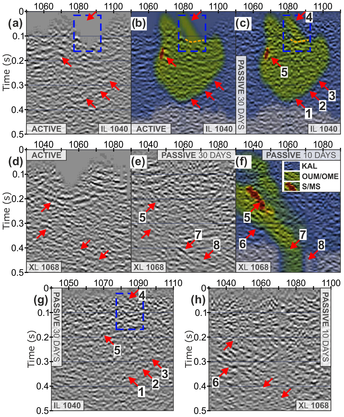
Figure 8Comparison of post-stack migrated sections obtained from the active and passive surveys. Inline 1040 (a–c, g) and crossline 1068 (d–f, h). (a–b, d) The active-source survey. (c, e, h) The 3D virtual-source survey. Red arrows mark the reflection events that are associated with the contacts in the geological model and confirmed with the active-source data. The arrows with numbers show reflections that are interpreted in the text. The geological model (described in Sect. 2) displayed in the background is color-coded as follows: S/MS mineralization (red); OUM/OME units (green); KAL unit (blue). Panels (g)–(h) show the same migrated stacks as in (c) and (f), respectively, but without the geological model and with a broader spatial extent.
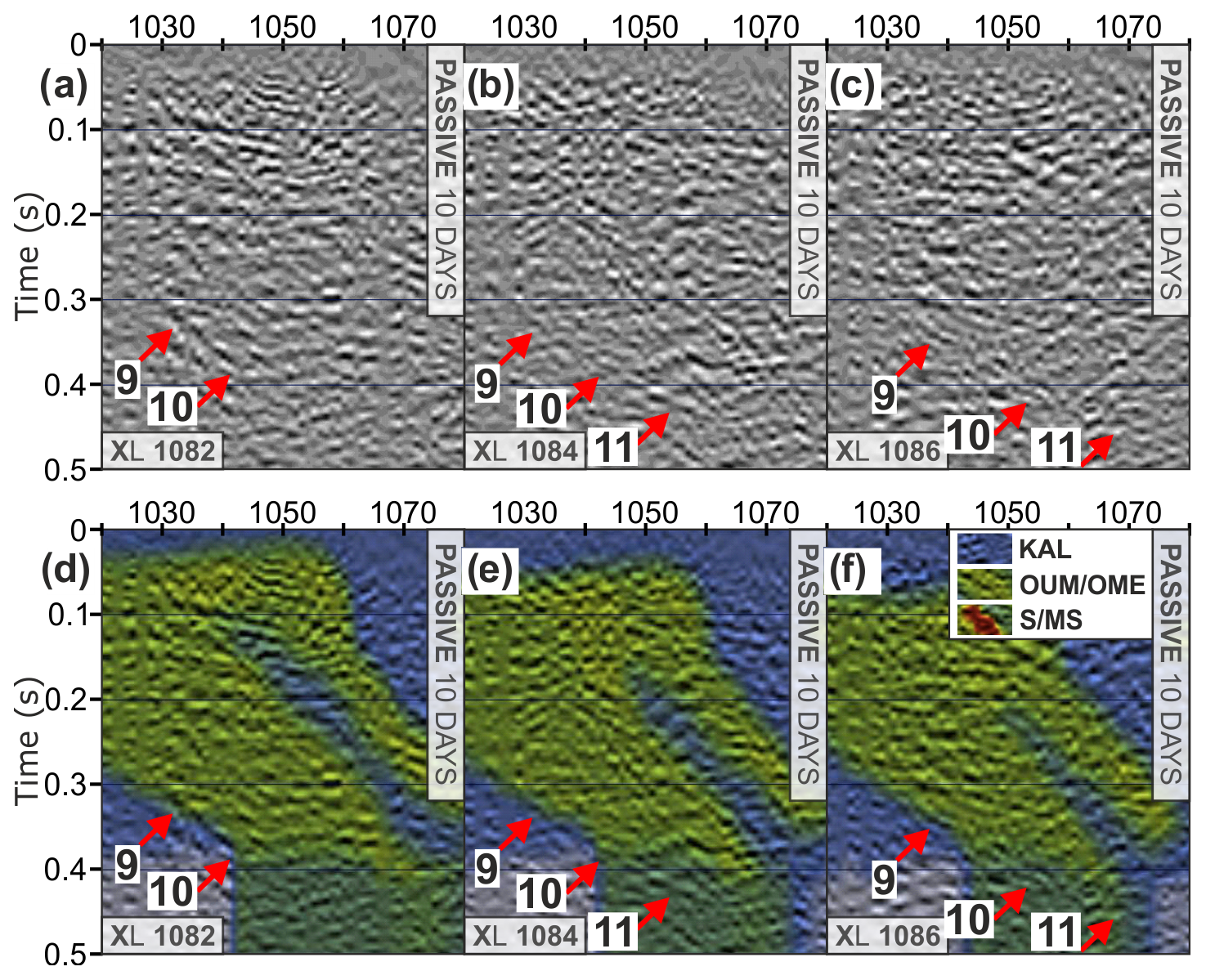
Figure 9Comparison of post-stack migrated sections obtained from the 3D virtual-source survey along crosslines 1082 (a, d), 1084 (b, d), and 1086 (c, f). Red arrows mark the reflection events that are associated with a key contact within the Kylylahti formation (OUM/OME in contact with black schists – KAL). Note that the extent of the geological model shown is constrained by the borehole data, and the marked reflections are at the very edge of this extent. The Kylylahti formation continues beyond the shown extent with further repetitions of the OUM/OME units with black schist interlayers. The arrows with numbers show reflections that are interpreted in the text. The geological model (described in Sect. 2) displayed in the background is color-coded as follows: S/MS mineralization (red); OUM/OME units (green); KAL unit (blue).
5.1 Ambient noise characteristics
AN characterization in this study was necessary to assess the temporal and spatial stationarity of the noise sources and confirm periods of data containing body-wave illumination. The spatial variability of AN in the Kylylahti area is mainly affected by the distance from the mine, and the temporal variability is mainly affected by the mine activity schedule. The secondary contributions are related to the presence of roads, and the city of Polvijärvi. In this study, we focus on the body-wave retrieval, and thus we put special emphasis on parts of the AN data that are characterized by AN in the higher-frequency range (see parts of PSDs associated with the frequency range 40–90 Hz in Fig. 3) and are mostly associated with seismic events with high apparent velocities (see the arrivals with velocities >4 km s−1 in the beamforming computed for the whole recording time in Fig. 4b). These features are mostly observed in the data recorded by receivers in the direct vicinity of the mine represented by area A1 in Fig. 1. However, as indicated in the PSD computed for the whole array (Fig. 3b) and the TWEED-detected body-wave events induced in the vicinity of the mine (Fig. 5a), the aforementioned spatial and temporal variations of AN should not preclude the retrieval of reflections from ANSI because most of the energy associated with body waves is recorded by the whole Kylylahti array. This is evidenced by the fact that higher-frequency content (>30 Hz) and body-wave events are observed even in the southernmost receiver lines of the Kylylahti array (receiver lines 15–19). These receiver lines are located furthest away from the mine (see areas A4 and A5 in Fig. 1) and are mostly influenced by road traffic. In the following, we discuss how these characteristics of the recorded noise affect the quality of the reflection content in VSGs.
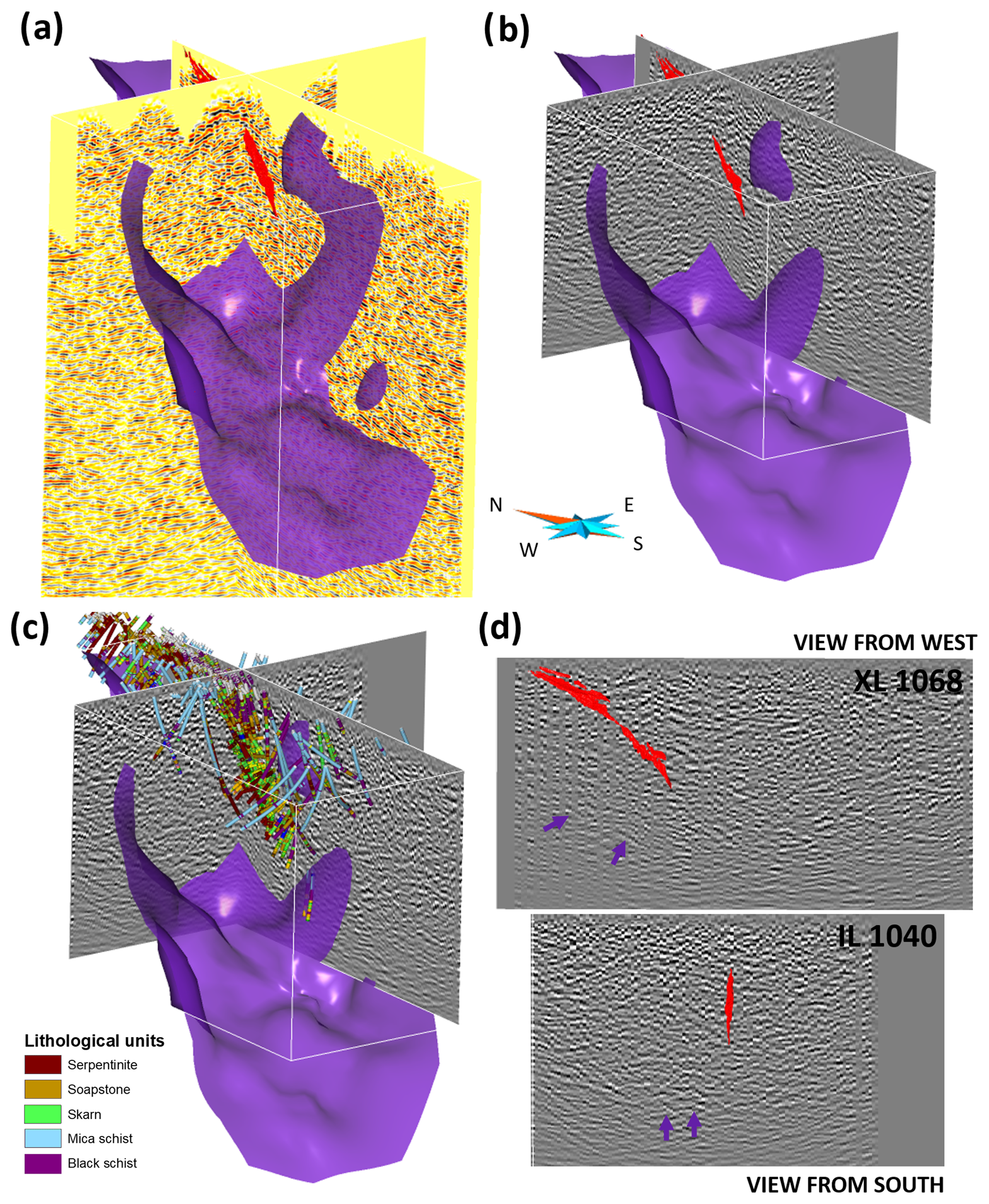
Figure 10(a) The Kylylahti active-source 3D data processed with a similar 3D reflection seismic processing workflow as the passive 3D 10 d subset data shown in (b) and overlapping the crossline 1068 and inline 1040 of the passive 3D cube in (b). The purple surface is the base of the Kylylahti formation interpreted from the COGITO-MIN 2D and 3D active-source data and the available borehole data (c). The red surface is the Kylylahti semi-massive to massive sulfide mineralization. (d) Reflection signals associated with the base of the Kylylahti formation on the crossline 1068 and inline 1040 of the passive 3D cube highlighted with purple arrows.
5.2 Impact of AN characteristics on VSG quality
The receivers that were used as master traces in Figs. 6–7 were selected to showcase the VSG quality obtained in different representative areas and based on the availability of co-located active-shot gathers. With this in mind, receiver stations 715, 1109, and 1556, due to their proximity to areas A1, A3, and A4 (see Fig. 1 for the location of the receivers and the corresponding areas), respectively, are strongly affected by certain AN sources: the mine (A1), a roundabout (A3), and a road (A4). This and the possible differences in the geophone coupling are the main reasons for differences observed in VSGs obtained for the same amount of data. As mentioned before, the computation of a single VSG involves cross-correlation of a master trace with each of the remaining 993 receivers, and thus the selection of a reference receiver has a huge impact on the quality of the VSGs. Consequently, any bias present in the data recorded by the master traces may influence every other trace in the VSG. To some extent, this explains why the relatively worst performance was obtained for the VSG for receiver location 1556 (Fig. 7), which according to the PSD computed for areas A4 and A5 (see Fig. 3a) is mostly affected by the road traffic AN. Nevertheless, due to the presence of higher frequencies, as well as the confirmed recording of events induced by the mine even at the furthest receiver lines (as evidenced in Fig. 5a), it was still possible to retrieve reflections, albeit with lower SNR. In addition to this, the differences between the VSGs (as well as the difference of correlated traces within a single VSG) obtained at different locations of the Kylylahti array were further remedied by spectral whitening and trace energy normalization (Draganov et al., 2013).
We conclude that the VSGs exhibit generally lower SNR compared to the co-located active-source data. On the other hand, the migrated sections of the passive data compared well to the sections from the active data (e.g., compare the active and passive image obtained for crossline 1068 shown in Fig. 8d and e, respectively). This was possible mainly due to feasibility of SI to provide passive reflections even at the receiver lines affected by road traffic (see, e.g., receiver line 15 in Fig. 7) and the higher number off all available virtual shots (994 VSGs versus only 736 active-source gathers) used for stacking.
5.3 ANSI processing with respect to the stationary-phase regions
From a data processing view, two things are crucial for SI reflection imaging: (i) the presence of body-wave sources and (ii) the fact that these sources must be located in the stationary-phase regions for reflection retrieval (Snieder, 2004; Draganov et al., 2006; Forghani and Snieder, 2010). The locations of the stationary-phase regions for reflection retrieval depend on the propagation velocity, position of the receivers, depth of the reflector, and the angle of incidence and reflection (Snieder, 2004; Mehta et al., 2008). Consequently, calculation of the region of the stationary-phase sources for a retrieval of a specific reflected wave between a virtual source and a receiver would require sufficiently accurate knowledge of the subsurface velocity model and an individual approach for every master–slave receiver pair. Therefore, beamforming, which incorporates summation over all receiver positions, may only serve as a general indicator of body-wave presence in the area, as well as a robust metric indicating whether these sources illuminate the target and Kylylahti area from multiple directions.
As shown in Fig. 5e, body-wave sources generated by the Kylylahti mine mostly occur in the subsurface. Consequently, the passive recordings from mining operations in the Kylylahti area can be used advantageously for retrieval of body-wave reflections with SI. When the majority of the sources are located in stationary-phase regions, the summation of the cross-correlated traces over all sources should result in retrieval of (kinematically) correctly located events without explicit subsurface velocity information (Schuster, 2001; Snieder, 2004; Brand et al., 2013). In this sense, the information provided by the beamforming indicates daily AN recordings dominated by presumed stationary-phase sources that, when stacked, ensure unaliased reflection arrivals in the VSGs.
As mentioned before, the decision of using daily AN recordings (rather than only noise panels with TWEED-detected events) was motivated by incorporating body-wave arrivals that were possibly not detected with TWEED (due to dominance of surface waves in the discarded panels but not necessarily a lack of body waves). Using all AN further increases the probability of capturing coda waves associated with body-wave arrivals and thus helps address one-sided illumination (we further discuss one-sided illumination in Sect. 5.5). As explained by Olivier et al. (2015), the coda waves in the active mine environment may be related to the mine tunnels that act as scatters. This creates the approximation of an inhomogeneous medium wherein seismic energy is scattered back to the receivers and effectively increases the number of stationary-phase regions. Note that coda waves due to weaker amplitudes can be at or below the noise level; therefore, the usability of coda waves for ANSI reflection imaging requires amplitude normalization.
5.4 Passive reflection images and interpretation
In order to validate the methodology presented in this work, the 3D passive seismic survey was purposefully accompanied with a 3D active-source survey and planned in an area for which detailed geological data were already available. The retrieval of reflection events in the VSGs and retrieval of an almost full reflection response of the complex Kylylahti formation in the migrated sections were possible mainly thanks to the favorable condition for SI highlighted in Sect. 4.1: primarily the abundance of subsurface sources (see Sect. 4.1.3), their approximate omnidirectional distribution (see Sect. 4.1.2), and relatively high frequencies (see Sect. 4.1.1). The discrepancies of the passive and active data observed in Figs. 6–9 arise mainly from compromising these factors during the stacking process for retrieval of VSGs: stacking VSGs obtained from all daily recordings possibly incorporates noise panels that were dominated by surface waves or were characterized by lower-frequency content (<35 Hz). Nevertheless, as shown by Dales et al. (2020), even AN sources located at the surface may contribute to retrieval of body-wave arrivals, and due to the constant presence of mine activity and the high-pass filtering (25–35–90–120 Hz), we assumed that body-wave arrivals will eventually outweigh the surface-wave content. This compromise, together with the local AN conditions affecting the master traces, as mentioned in the previous subsection, is evidenced in Figs. 6–7. The retrieved VSGs exhibit relatively lower SNR than the active data, as well as varying quality between passive reflections visible in the stacks for the same amount of data, but different master traces. Still, the migrated images from the active and passive surveys are consistent in terms of general dip of the refection events, as well as the reflections related to internal contacts within the Kylylahti formation. Due to the high quality of the migrated sections, we suspect that artifacts identified in the off-end lines (see, e.g., black arrows in Fig. 7) were suppressed during stacking of all 994 shots, and thus possible weak reflectivity was uncovered.
To highlight the main benefits that passive seismic can provide in active mine environments we chose representative inlines and crosslines from the 3D passive cube that (i) show consistent retrieval of the internal contacts within the Kylylahti formation (general structural delineation). Specifically, we highlight here that the reflections predicted by the geological model and associated with a contact between the OUM/OME unit and black schists (KAL) within the Kylylahti formation were imaged in both inline and crossline directions of the passive survey and exhibit a coherent and continuous nature comparable with the quality of active data. The representative inlines and crosslines also (ii) provide a reflection response in the areas where active data are not available (passive data can supplement or complete images from the active data) and (iii) have the potential to indicate new prospective areas, with reflections extending beyond the known extent of these contacts (based on the geological model derived from the borehole data). The continuous dipping reflection was retrieved in three consecutive crosslines (crosslines 1082, 1084, 1086 in Fig. 9). The same dipping reflection in the crossline 1084 (Fig. 9e) appears to extend further in the inline direction of the passive cube.
However, we emphasize that the above features of the passive method are only achievable when either active-source data are available or an approximate velocity model of the target is available. Nevertheless, this requirement does not harm the benefits of ANSI highlighted in this study. In particular, in similar complex environments also characterized by significant thickness variations of the low-velocity overburden layer on the top of the high-velocity bedrock, static corrections are crucial for extracting a coherent reflection response. In our case, the refraction static corrections applied to the passive data were obtained from the active-source data. It should be noted that in the case of a passive survey only, the shallow low-velocity layer model required for calculation of the statics should then be obtained by some other means, e.g., via a separate refraction seismic survey or surface-wave analysis.
5.5 The essence of creating two subsets of VSGs
The usual approach of improving reflections retrieved using ANSI relies on increasing the passive acquisition time so that a higher number of noise panels may be used to retrieve VSGs. This is explained by the fact that longer monitoring could increase the chance of accumulating noise sources with a greater diversity of ray parameters, implying more comprehensive illumination of the array (Draganov et al., 2013). On the other hand, as explained by Draganov et al. (2006) and Forghani and Snieder (2010) only sources that are located in the stationary-phase regions constructively contribute to the reflection retrieval. As evidenced in daily beamforming plots (Fig. 4a), the AN from Kylylahti is characterized by changes in the temporal (daily variations) and spatial (directivity changes) stationarity of noise sources. This means that including more data may actually obscure the retrieved reflection events through interference with retrieved artifacts, while stacking smaller amounts of data might result in retrieval of reflections with higher SNR. This observation becomes more evident when the source distribution is imperfect, for instance when sources are clustered in specific places of the recording area. Therefore, contrary to the conventional approach used in ANSI, i.e., recording as much noise as possible and then stacking all the noise panels (e.g., Cheraghi et al., 2015; Chamarczuk et al., 2018), one needs to be more selective in the stacking process.
For the Kylylahti case study, the beamforming analysis indicated the possibility to obtain broad azimuthal coverage of body-wave arrivals using only days dominated by body-wave arrivals. However, the beamforming analysis also indicated the presence of body-wave arrivals during days dominated by surface waves. This showed us that the feasibility of using SI with the Kylylahti array should be investigated using two approaches: using all data and using a subset of recordings containing only days dominated by body-wave arrivals. While the latter allowed for the examination of the potential of reflection retrieval less biased by surface-wave content in a computationally efficient manner, stacking over all days (including those dominated by surface-wave arrivals) should yield more omnidirectional coverage resulting from including body-wave sources that illuminate from azimuths not covered in the subset of 10 d.
In this study, we used the subset of 10 d of AN recordings as the representation of the selective stacking approach. This subset was selected based on TWEED using information from the PSD and the beamforming, and it represents the practical trade-off between the minimum number of AN recordings required to obtain daily records with body-wave arrivals that altogether form the omnidirectional contour created by arrivals from different azimuths (note the changing angle of high-velocity maxima inside the beamforming results highlighted with a green circle in Fig. 4a). As explained in Sect. 4.1.3, the data from the selected 10 d contain sources that are clustered mostly inside the mine area (Fig. 5d) and are distributed along approximately a vertical column slightly shifted to the right with respect to the mine location (Fig. 5e). For this reason, the imaging results obtained for the 10 d of AN contain several differences compared to the all-data results imposed by the one-directional source distribution. However, as explained by Wapenaar (2006), even when the sources exhibit a one-sided distribution it is still possible to retrieve reflectivity using SI, and consequently the discrepancies between the 10 and 30 d stacks are theoretically justified. We note here that the one-directional illumination would be a typical issue for VSSs conducted above underground mines, where the most of the seismic activity is in the direct vicinity of the mine operations (Chamarczuk et al., 2021).
5.6 Differences in the 10 and 30 d passive imaging approaches and the active-source imaging
As a part of the reconnaissance ANSI study in the Kylylahti area (Chamarczuk et al., 2021), we investigated the implications of a one-sided source distribution for the specific configuration of the Kylylahti case study by performing synthetic studies. These tests were undertaken to (i) investigate the influence of AN sources distributed along one of the three sides of the Kylylahti formation and (ii) to aid the interpretation of the migrated passive field data by explaining artifacts related to directional source distributions.
According to the findings, when clusters of sources are predominantly focused in some area (i.e., scenario violating the omnidirectional distribution) it is still possible to image a part of the Kylylahti deposit. As explained above, the sources included in the selected 10 d are clustered in the center of the total distribution of all sources (compare the distribution of black and red dots in Fig. 5d–e) with slight deviation to the right flank of the mine area as well as of the Kylylahti formation. The synthetic tests (Chamarczuk et al., 2021) showed that migrated sections obtained from directionally biased source distributions are generally dominated by artifacts, but it is still possible to track the reflectivity in the expected areas. The comparison of migrated images using sources distributed to the left, underneath, and on the right flank of the target revealed that the relatively lowest-quality image is provided using sources distributed along the right side of the target, with a prominent horizontal artifact that masks the reflection packages related to part of the target with high impedance inclusions. On the other hand, sources distributed on the right flank exhibited the highest level of SNR in the area between the reflection packages and clear reflection from the prominent contact between the OUM/OME unit and black schists (KAL) within the Kylylahti formation, which is the case for the passive results shown in Figs. 8 and 9.
As highlighted before, selective stacking can be used to extract only recordings that are dominated by stationary-phase sources. When all data are stacked, the risk of incorporating sources that are not located in stationary-phase regions, and/or are dominated by surface-wave arrivals may lead to obscuring the retrieved reflection arrivals due to destructive interference. As shown in stacked beamforming output (Fig. 4b), using all data provides body-wave arrivals with an omnidirectional distribution; however, the inspection of the beamforming plots from individual days (Fig. 4a) suggests that the same approach inherently incorporates undesired surface-wave arrivals. Our approach to remedy this issue relied on the application of spectral whitening to first enhance the weak body-wave arrivals associated with time periods when mine-induced noise was dominated by road traffic, followed by bandpass filtering that aimed to reject the surface waves. The results from 30 d, as opposed to 10 d stack, exhibit generally more reflectivity due to stacking over body-wave arrivals with a more uniform angle distribution. However, due to the presence of surface waves not fully suppressed by the preprocessing and incorporation of body-wave sources outside stationary-phase regions, the results from all data exhibit reflection arrivals that have lower SNR compared to the results from stacking only days when the body waves were dominant.
We investigated the imaging potential of the large-N passive seismic array for near-mine exploration in conjunction with the developed methodology for body-wave reflection retrieval using seismic interferometry. The core of our workflow is a combination of the standard tools used to describe AN (PSD, beamforming) with a novel form of illumination diagnosis and noise-source location to verify and extract actual body-wave events. Selective stacking is typically required to ensure successful retrieval of body-wave arrivals with preferential illumination. In this case, we selectively stacked 10 d of data dominated by omnidirectional body-wave energy. This approach was compared to an all-noise approach with stacking of all 30 d of data. While the 10 d approach is better at resolving the continuity of some key reflections, the 30 d approach produced generally similar results. We conclude that understanding the AN characteristic is key for choosing a data-driven stacking approach that best suits the specifics of the data and the target. By comparing the results of the passive seismic survey to active-source seismic data and pre-existing detailed geological models from the target area, this first hardrock full-scale 3D passive experiment confirmed the feasibility of virtual-source surveys to provide interpretable reflection images of structures beyond the known extent of the prospective zones. As such, the methodology has potential to guide exploration drilling efforts at lower total acquisition costs, as confirmed by some earlier passive seismic studies. The specific added value of this study is the demonstration of the value of ANSI in the full-scale 3D configuration. The Kylylahti passive experiment highlights the potential of active mine environments to generate ambient noise useful for imaging. Our methodology can also be used beyond the mineral exploration context, e.g., for geothermal exploration in crystalline rocks, with the noise sources expected to be located below the array.
All passive results presented in this study (two sets of virtual-source gathers and migrated sections) are freely available through the Finnish Fairdata services: https://doi.org/10.23729/8469939b-4abe-405e-9eeb-53016acdfb7d (Chamarczuk and Koivisto, 2021). The original raw and unprocessed ambient noise recordings, which consist of the whole recorded data volume (600 h for 994 receiver stations), are freely available through the Finnish Fairdata services: https://doi.org/10.23729/48acb337-3be0-4e76-94f9-5e60779c26fe (Chamarczuk, 2021). The approximate size of this repository is 3.74 TB, and there are additional files that explain all details about storage and understanding of the data towards simplification of processing. The GOCAD® Mining Suite was used to create the 3D visualization shown in Fig. 10.
MCH wrote the original paper draft, with contributions from all the authors (with substantial contributions provided by MM, DD, and EK). MM, EK, and SH designed the field acquisition of passive and active seismic experiments. MCH, MM, EK, SH, and SR participated in the fieldwork supervised and coordinated by EK, SH, and MM. MCH conceptualized and developed the methodology of ambient noise data processing and applied it to the field data from Kylylahti under the coordination and supervision of DD and MM. MM and MCH contributed to the processing of the active-source data. EK provided interpretation of the 3D seismic data. EK and SR provided geological models and their interpretation. SR provided expertise and support with respect to all information related to the Kylylahti mine. MCH and EK created and submitted datasets to online repositories, which are linked from this paper. All authors contributed to the countless discussions of the results.
The contact author has declared that neither they nor their co-authors have any competing interests.
This article is part of the special issue “State of the art in mineral exploration”. It is a result of the EGU General Assembly 2020, 3–8 May 2020.
Publisher's note: Copernicus Publications remains neutral with regard to jurisdictional claims in published maps and institutional affiliations.
We thank the field crews from the University of Helsinki, Geological Survey of Finland, IG PAS, and Boliden for deploying the Kylylahti array. We also specifically thank Novaseis for their field support during the data acquisition. We thank two anonymous reviewers for their thorough reading of our paper and many detailed comments, which allowed us to improve the paper.
This research has been supported by the Business Finland (grant agreement no. ERA-MIN/COGITO-MIN/3704/31/2015) and the National Center for Research and Development (NCBR) (grant agreement no. ERA-MIN/COGITO-MIN/01/2016).
This paper was edited by Juan Alcalde and reviewed by two anonymous referees.
Ben-Zion, Y., Vernon, F. L., Ozakin, Y., Zigone, D., Ross, Z. E., Meng, H., and Barklage, M.: Basic data features and results from a spatially dense seismic array on the San Jacinto fault zone, Geophys. J. Int., 202, 370–380, https://doi.org/10.1093/gji/ggv142, 2015.
Chamarczuk, M.: Kylylahti 3D virtual seismic survey (unprocessed ambient-noise recordings), Version 2, Fairdata.fi [data set], https://doi.org/10.23729/48acb337-3be0-4e76-94f9-5e60779c26fe, 2021.
Chamarczuk, M. and Koivisto, E.: Kylylahti 3D virtual seismic survey, Version 1, Fairdata.fi [data set], https://doi.org/10.23729/8469939b-4abe-405e-9eeb-53016acdfb7d, 2021.
Chamarczuk, M., Malinowski, M., Koivisto, E., Heinonen, S., Juurela, S., and COGITO-MIN Working, G.: Passive seismic interferometry for subsurface imaging in an active mine environment: case study from the Kylylahti Cu-Au-Zn mine, Finland, Proceedings of Exploration'17: Seismic Methods and Exploration Workshop, 2017, 1–56, 2017.
Chamarczuk, M., Malinowski, M., Draganov, D., Koivisto, E., Heinonen, S., and Juurela, S.: Seismic Interferometry for Mineral Exploration: Passive Seismic Experiment over Kylylahti Mine Area, Finland, Eur. Assoc. Geosci. Eng., 2018, 1–5, https://doi.org/10.3997/2214-4609.201802703, 2018.
Chamarczuk, M., Malinowski, M., Nishitsuji, Y., Thorbecke, J., Koivisto, E., Heinonen, S., Mezyk, M., Juurela, S., and Draganov, D.: Automatic 3D illumination diagnosis method for large-N arrays: robust data scanner and machine learning feature provider, Geophysics, 84, 13–25, https://doi.org/10.1190/geo2018-0504.1, 2019.
Chamarczuk, M., Nishitsuji, Y., Malinowski, M., and Draganov, D.: Unsupervised learning used in automatic detection and classification of ambient-noise recordings from a large-n array, Seismol. Res. Lett., 91, 370–389, https://doi.org/10.1785/789 0220190063, 2020.
Chamarczuk, M., Malinowski, M., and Draganov, D.: 2D body-wave seismic interferometry as a tool for reconnaissance studies and optimization of passive reflection seismic surveys in hardrock environments, J. Appl. Geophy., 187, 104288, https://doi.org/10.1016/j.jappgeo.2021.104288, 2021.
Cheraghi, S., Craven, J. A., and Bellefleur, G.: Feasibility of virtual source reflection seismology using interferometry for mineral exploration: A test study in the Lalor Lake volcanogenic massive sulphide mining area, Manitoba, Canada, Geophys. Prospect., 63, 833–848, https://doi.org/10.1002/2015JB011870, 2015.
Dales, P., Audet, P., Olivier, G., and Mercier, J. P.: Interferometric methods for spatio-temporal seismic monitoring in underground mines, Geophys. J. Int., 210, 731–742, https://doi.org/10.1093/gji/ggx189, 2017.
Dales, P., Pinzon-Ricon, L., Brenguier, F., Boué, P., Arndt, N., McBride, J., and Olivier, G.: Virtual Sources of Body Waves from Noise Correlations in a Mineral Exploration Context, Seismol. Res. Lett., 91, 2278–2286, https://doi.org/10.1785/0220200023, 2020.
Daneshvar, M. R., Clay, C. S., and Savage, M. K.: Passive seismic imaging using microearthquakes, Seismol. Res. Lett., 60, 1178–1186, https://doi.org/10.1190/1.1443846, 1995.
Draganov, D., Wapenaar, K., and Thorbecke, J.: Seismic interferometry: reconstructing the Earth's reflection response, Geophysics, 71, 61–170, https://doi.org/10.1190/1.2209947, 2006.
Draganov, D., Campman, X., Thorbecke, J., Verdel, A., and Wapenaar, K.: Reflection images from ambient seismic noise, Geophysics, 74, 63–67, https://doi.org/10.1190/1.3193529, 2009.
Draganov, D., Campman, X., Thorbecke, J., Verdel, A., and Wapenaar, K.: Seismic exploration-scale velocities and structure from ambient seismic noise (>1 Hz), J. Geophys. Res.-Sol. Ea., 118, 4345–4360, https://doi.org/10.1002/jgrb.50339, 2013.
Forghani, F. and Snieder, R.: Underestimation of body waves and feasibility of surface-wave reconstruction by seismic interferometry, Lead. Edge, 29, 790–794, https://doi.org/10.1190/1.3462779, 2010.
Heinonen, S., Malinowski, M., Hloušek, F., Gislason, G., Buske, S., Koivisto, E., and Wojdyla, M.: Cost-effective seismic exploration: 2D reflection imaging of the mineral system of Kylylahti, Easter Finland, Minerals, 9, 263, https://doi.org/10.3390/min9050263, 2019.
Koivisto, E., Malinowski, M., Heinonen, S., Cosma, C., Wojdyla, M., Vaittinen, K., and the COGITO-MIN Working Group: From Regional Seismics to High-Resolution Resource Delineation: Example from the Outokumpu Ore District, Eastern Finland, European Association of Geoscientists and Engineers, 2018, 1–5, https://doi.org/10.3997/2214-4609.201802716, 2018.
Luhta, T.: Petrophysical properties of the Kylylahti Cu-Au-Zn sulphide mineralization and its host rocks, Master's thesis, University of Helsinki, Finland, https://helda.helsinki.fi/handle/10138/302130 (last access: 11 March 2022), 2019.
Mehta, M., Snieder, R., Calvert, R., and Sheiman, J.: Acquisition geometry requirements for generating virtual-source data, Lead. Edge, 27, 620–629, https://doi.org/10.1190/1.2919580, 2008.
Nakata, N., Chang, J. P., Lawrence, J., and Boué, P.: Body wave extraction and tomography at long beach, California, with ambient-noise interferometry, J. Geophys. Res.-Sol. Ea., 120, 1159–1173, https://doi.org/10.1002/2015JB011870, 2015.
Olivier, G., Brenguier, F., Campillo, M., Lynch, R., and Roux, P.: Body-wave reconstruction from ambient noise seismic noise correlations in an underground mine, Geophysics, 80, 11–25, https://doi.org/10.1190/geo2014-0299.1, 2015.
Peltonen, P., Kontinen, A., Huhma, H., and Kuronen, U.: Outokumpu revisited: New mineral deposit model for the mantle peridotite-associated Cu-Co-Zn-Ni-Ag-Au sulphide deposits, Ore Geol. Rev., 33, 559–617, https://doi.org/10.1016/j.oregeorev.2007.07.002, 2008.
Quiros, D., Brown, L., and Doyeon, K.: Seismic interferometry of railroad induced ground motions: body and surface wave imaging, Geophys. J. Int., 205, 301–313, https://doi.org/10.1093/gji/ggw033, 2016.
Riedel, M., Cosma, C., Enescu, N., Koivisto, E., Komminaho, K., Vaittinen, K., and Malinowski, M.: Underground Vertical Seismic Profiling with Conventional and Fiber-Optic Systems for Exploration in the Kylylahti Polymetallic Mine, Eastern Fin Land, Minerals, 8, 538, https://doi.org/10.3390/min8110538, 2018.
Roots, E., Calvert, A., and Craven, J.: Interferometric seismic imaging around the active Lalor mine in the Flin Flon greenstone belt, Canada, Tectonophysics, 718, 92–104, https://doi.org/10.1016/j.tecto.2017.04.024, 2017.
Rost, S. and Thomas, C.: Array seismology: Methods and applications, Rev. Geophys., 40, 1–27, https://doi.org/10.1029/2000RG000100, 2002.
Ruigrok, E., Campman, X., Draganov, D., and Wapenaar, K.: High-resolution lithospheric imaging with seismic interferometry, Geophys. J. Int., 183, 339–357, https://doi.org/10.1111/j.1365-246X.2010.04724.x, 2010.
Ryberg, T.: Body wave observations from cross-correlations of ambient seismic noise: A case study from the Karoo, RSA, Geophys. Res. Lett., 38, L13311, https://doi.org/10.1029/2011GL047665, 2011.
Schuster, H.: Theory of daylight/interferometric imaging: tutorial, Extended Abstracts, European Association of Geoscientists and Engineers, https://doi.org/10.3997/2214-4609-pdb.15.A-32, 2001.
Singh, B., Malinowski, M., Hloušek, F., Koivisto, E., Heinonen, S., Hellwig, O., and Juurela, S.: Sparse 3D Seismic Imaging in the Kylylahti Mine Area, Eastern Finland: Comparison of Time vs Depth Approach, Minerals, 9, 305, https://doi.org/10.3390/min9050305, 2019.
Snieder, R.: Extracting the green's function from the correlation of coda waves: a derivation based on stationary phase, Phys. Rev. E, 69, 46610, https://doi.org/10.1103/PhysRevE.69.046610, 2004.
Väkevä, S.: Using Three-Component Data for Seismic Interferometry Studies at the Kylylahti Mine, Master's thesis, University of Helsinki, Finland, https://helda.helsinki.fi/handle/10138/302127 (last access: 11 March 2022), 2019.
Wapenaar, K.: Green's function retrieval by cross-correlation in case of one-sided illumination, Geophys. Res. Lett., 33, L19304, https://doi.org/10.1029/2006GL027747, 2006.